Tunneling time, the barrier time-delay and weak measurement
What was or can actually be measured with the Attoclock?

Abstract

The measurement of the tunneling time-delay in attosecond experiments, termed attoclock, despite its controversies, offers a fruitful opportunity to understand the tunneling time and the tunnel-ionization process. In previous work, we showed a model that well describes the time-delay measured by the attoclock experiment in the adiabatic and nonadiabatic field calibrations. In the present work we show that the tunneling time reveals a universal behavior, with disentangled contribution, where the barrier time-delay can be convincingly defined and determined from the difference between the time-delay of adiabatic and nonadiabatic tunnel-ionization, with good agreement with the experimental result. Furthermore, we show that in the weak measurement limit, the barrier time-delay corresponds to the Larmor-clock time and the interaction time within the barrier.

.1 Theoretical model

The interaction of an atom with laser pulse in the strong-field and attosecond science can be modeled in a simplified picture as shown in fig. 1. With its help, we developed a simple tunneling model in Kullie (2015) with expressions composed of basic laser and atomic parameters that describes the measurement result of the attocolck. The model provides a new insights into temporal property of tunneling ionization, and shed light on roles of time in quantum mechanics. Below we briefly present our model, in which an electron can be tunnel-ionized by a laser pulse with an electric field strength (hereafter field strength) $F$. A direct ionization happen when the field strength reaches a threshold called atomic field strength $F_{a}=I_{p}^{2}/(4Z_{eff})$ Augst et al. (1989, 1991), where $I_{p}$ is the ionization potential of the system (atom or molecule) and $Z_{eff}$ is the effective nuclear charge in the single-active electron approximation (SAEA). We adopt in this work the atomic units ($au$), where the mass and charge of the electron as well as the Planck constant set to unity, $\hbar=m=e=1$. However, for $F<F_{a}$ the ionization can happen by tunneling through a potential barrier of an effective potential consisting of the Coulomb potential of the core and the electric field of the laser pulse. It can be expressed in a one-dimensional form by

$$V_{eff}(x)=V(x)-xF=-\frac{Z_{eff}}{x}-xF,$$ (1)

compare fig. 1. In the model the tunneling process can be described solely by the ionization potential $I_{p}$ of the valence (the interacting) electron and the peak field strength $F$ with the barrier height is given by $\delta_{z}=\sqrt{I_{p}^{2}-4Z_{eff}F}$, where $F$ stands (throughout this work) for the peak electric field strength at maximum. In fig. 1 (for details see Kullie (2015)), the inner (entrance $x_{e,-}$) and outer (exit $x_{e,+}$) points are given by $x_{e,\pm}=(I_{p}\pm\delta_{z})/(2F)$, the barrier width is $d_{B}=x_{e,+}-x_{e,-}=\delta_{z}/F$, and its (maximum) height (at $x_{m}(F)=\sqrt{Z_{eff}/F}$) is $\delta_{z}$. At $F=F_{a}$, we have $\delta_{z}=0$ ($d_{B}=0$), the barrier disappears and the direct or the barrier-suppression ionization starts, green (dashed-doted) curve in fig.1 .

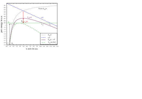
Figure 1: (Color online) A sketch of the atomic and the effective potential curves, showing the height and width of the barrier formed by the laser field. The plot is for He-atom in the SAEA model with $Z_{eff}=1.6875$ and $I_{p}\approx 0.9\,au$.

Adiabatic tunneling:

In the adiabatic field calibration of the attoclock of Landsman et. al. Landsman et al. (2014), we showed in Kullie (2015) that the tunneling time-delay is expressed by the forms,

$$\tau_{{}_{T,d}}=\frac{1}{2(Ip-\delta_{z})},\quad\tau_{{}_{T,i}}=\frac{1}{2(I_{p}+\delta_{z})}$$ (2)

It was shown Kullie (2015) that $\tau_{{}_{T,d}}$ agrees well with the experimental result of Landsman et. al. Landsman et al. (2014) . Their physical reasoning is the following: $\tau_{{}_{T,d}}$ is the time-delay of the adiabatic tunnel-ionization with respect to the ionization at atomic field strength $F_{a}$ required to overcome the barrier and escape at the exit point $x_{e,+}$ into the continuum Kullie (2015). Whereas $\tau_{{}_{T,i}}$ is the time needed to reach the entrance point $x_{{}_{e,-}}$ from the initial point $x_{i}$, compare fig. 1. At the limit of atomic field strength, we have $\lim\limits_{F\to F_{a}}(\delta_{z}\to 0)\tau_{{}_{T,d}}=\frac{1}{2Ip}=\tau_{a}$ (see below). For $F>F_{a}$, the barrier-suppression ionization sets up Delone and Kraǐnov (1998); Kiyan and Kraǐnov (1991). On the opposite side, we have $\lim\limits_{F\to 0}(\delta_{z}\to I_{p})\tau_{{}_{T,d}}\to\infty$. So nothing happens and the electron remains in its ground state undisturbed, which shows that our model is consistent. For details, see Kullie (2015, 2016, 2018, 2020).

Nonadiabatic tunneling:

In the nonadiabatic field calibration of Hofmann et. al. Hofmann et al. (2019), we found in Kullie (2024) that the time-delay of the nonadiabatic tunnel-ionization is descried by

$$\tau_{dion}(F) = \frac{1}{2I_{p}}\frac{F_{a}}{F}=\tau_{a}\xi_{F}$$ (3)

In Kullie (2024) it was shown that 3 agrees well with the experimental result of Hofmann et. al. Hofmann et al. (2019). In addition, the result was confirmed by the numerical integration of the time-dependent Schrödinger equation (NITDSE) Kullie (2024). It is easily seen that in the limit $F\to F_{a},\tau_{dion}=\tau_{a}$, whereas in the opposite case $F\to 0,\tau_{dion}=\infty$. $\tau_{a}$ is always (adiabatic and nonadiabatic) a lower quantum limit of the tunnel-ionization time-delay and quantum mechanically does not vanish. $\xi(F)$ is an enhancement factor for field strength $F<F_{a}$.

.2 The barrier time-delay

In this section, we show that the time-delay due to the barrier itself, which is the actual tunneling time-delay can be determined by considering the adiabatic and nonadiabatic field calibrations together. Eq 2 can be decomposed into a twofold time-delay with respect to ionization at $F_{a}$, representing $\tau_{{}_{T,d}}$ in an unfolded form,

$$\tau_{{}_{T,d}} = \frac{1}{2(Ip-\delta_{z})}=\frac{1}{2}\frac{I_{p}}{4Z_{eff}F}\left(1+\frac{\delta_{z}}{I_{p}}\right)$$

$$= \frac{1}{2I_{p}}\frac{F_{a}}{F}\left(1+\frac{\delta_{z}}{I_{p}}\right)=\tau_{a}(\xi_{F}(F)+\Lambda_{F}(F))$$

$$= \tau_{dion}+\tau_{delt}\equiv\tau_{Ad}$$

Below we refer to it as adiabatic tunnel-ionization $\tau_{Ad}$. Eq. .2 immediately shows in the second line that the adiabatic time-delay can be easily interpreted as a time-delay with respect to ionization at atomic field strength $\tau_{a}=\tau_{{Ad}}(F_{a})=1/(2I_{p})$, where both terms present real time-delay. And again $(\xi_{F}+\Lambda_{F})$ is an enhancement factor for field strength $F<F_{a}$. The first term of $\tau_{dion}$ eq. .2, which is the same of eq. 3, is a time-delay solely because $F$ is smaller than $F_{a}$, whereas the second term $\tau_{delt}$ is a time-delay due to the barrier itself, it is the actual tunneling time-delay Kullie (2020). This can be seen form the factor ${\delta_{z}}/{I_{p}}$, which vanishes for $F=F_{a}$ when the barrier disappears $\delta_{z}=0$

Indeed, Winful Winful (2003) and Lunardi Lunardi and Manzoni (2019) proposed a similar unfolded form to the adiabatic tunnel-ionization time-delay given in eq. .2.

$$\tau^{Winf}_{g} = \tau_{si}+\tau_{dwell}$$ (5)

$$\tau^{Lun}_{T} = \tau_{well}+\tau_{barrier}$$ (6)

In the quantum tunneling of a wave packet or a flux of particles scattering on a potential barrier, Winful showed that the group time-delay or the Wigner time-delay can be written in the form 5, where $\tau_{dwell}$ is the dwell time which corresponds to our $\tau_{delt}$, and $\tau_{si}$ is according to Winful a self-interference term, which corresponds to our $\tau_{ion}$. Importantly, Winful showed that the contribution of the first term is disentangled from the barrier time-delay Winful (2003). And in their work Lunardi et. al. used the so-called Slacker-Wigner-Peres quantum-clock (SWP-QC) with MC-simulation Lunardi and Manzoni (2018, 2019), they found that the tunneling time in the attoclock is given by the form 6

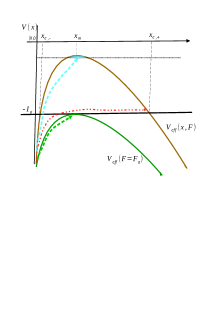
Figure 2: (Color online) Illustration of tunnel-ionization of the horizontal (dashed-dotted, red) and vertical (dashed, blue) channels. The dotted line is a virtual state. As well as the BSI (green). Compare fig. 1

The author called the first term well-time and, according to the authors, is the time (-delay) spent before reaching the barrier and suggest that the second term corresponds to the barrier time (-delay). The three results (ours confirmed with the NITDSE, Winful’s and Lunardi’s) clearly show that the separation of eq. .2 presents a unified T-time picture (UTTP) Winful (2003), allowing us to conclude that the time-delay due the barrier itself is giving by $\tau_{delt}=\tau_{dwell}=\tau_{barrier}$, which can be determined form eqs 3, .2

$$\tau_{{}_{Ad}}-\tau_{dion}=\tau_{delt}=\frac{1}{2}\frac{1}{4Z_{eff}}\frac{\delta_{z}}{F}=\frac{1}{2}\frac{d_{B}}{4Z_{eff}}$$ (7)

Eq 7 $\tau_{delt}$ is the barrier time-delay, usually referred to as the time spent within the barrier $\tau_{barrier}$ or the dwell time $\tau_{dwell}$. One also finds a linear dependence of $\tau_{delt}$ on the barrier width $d_{B}$, The barrier time-delay tends to zero in the limit of $F=F_{a}(\delta_{z}=d_{B}=0)$ because the barrier disappears, as is known from the seminal work of Hartman Hartman (1962). Obviously, $\tau_{delt}$ cannot be measured by the experiment directly since the first term is always present, $\tau_{si},\tau_{well},\tau_{dion}$. However, as seen in eq. 7, it can be determined taking both field calibrations into account. An illustration of the tunnel-ionization of adiabatic (horizontal) and nonadiabatic (vertical) channels is shown in for fig. 2. Fortunately, for the He-atom we can consider the results of Landsman Landsman et al. (2014) (adiabatic calibration) and Hofmann Hofmann et al. (2019) (nonadiabatic calibration) since they belong to the same experiment Eckle et al. (2008a, b). In fig. 3 (left), we show both experimental results with curves obtained by data fitting. The curves show a $1/F$-dependence as expected, subtracting them from each other gives the experimental barrier time $\tau_{barrier,exp}$. In fig. 3 (right), we compare the barrier time-delay $\tau_{delt}$ of eq. 7 with $\tau_{barrier,exp}$. We plot $\tau_{delt}$ for two $Z_{eff}=1.0,1.344=\sqrt{2I_{p}}$, expanding the range to a larger barrier width (smaller $F$) than specified in the experimental data. As can be seen in fig. 3, the agreement is very good. It undoubtedly shows that the time spent in the barrier (or time-delay caused by the barrier upon tunnel-ionization of the electron) is $\tau_{delt}$, which can be determined from the experimental data by $\tau_{barrier,exp}$. The agreement becomes better for $Z_{eff}=1$ in the region of small field strength, because the barrier width $d_{B}=\delta_{z}/F$ is large and the tunnel-ionized electron escapes far from the atomic core. Whereas for larger field strength (near the atomic field strength) the barrier width is small and the agreement is better for $Z_{eff}=\sqrt{2I_{p}}=1.344$. Finally, all curves tends to zero for $F\rightarrow F_{a}$, because the barrier disappears, as already mentioned and should be. Additionally, we plot in fig. 3 a curve ($\tau_{LC}$) of Larmor clock (LC) time, which is also obtained by fitting the LC data given by Hofmann Hofmann et al. (2019). The agreement with LC is better for small $F$ values, which is the limit of thick barrier (more on this in the next section). This is because Hofmann’s LC time-delay is given for the nonadiabatic field calibration and our $\tau_{delt}$ becomes closer to nonadiabatic time-delay $\tau_{dion}$ for small $F$ (thick barrier) (see eq. 8 below), which again explains the disagreement for larger field strength $F=0.06-0.1$, compare fig. 3. Below the notation $\tau_{delt}$ is used to refer to the barrier time-delay $\tau_{delt}(\equiv\tau_{barrier}\equiv\tau_{dwell})$, with the corresponding adiabatic and nonadiabatic tunnel-ionization time-delay $\tau_{Ad}$, $\tau_{dion}$, respectively.

.3 The weak measurement and the interaction time

In the previous section we found that the LC time $\tau_{LC}$ tends closer to the barrier time-delay $\tau_{delt},\,\tau_{barrier,exp}$ for small field strength, compare fig. 3 (right). The LC-time is usually considered in the context of the so-called weak measurement (WM) approach, which characterize a system before and after it interacts with a measurement apparatus Aharonov et al. (1988); Rozema et al. (2012). WM does not significantly perturbs the system, where Landsman Landsman and Keller (2015) showed that the WM value of the time-delay corresponds to LC-time $\tau_{weak}=\tau_{LC}$ Landsman and Keller (2015); Steinberg (1995). Thus, for small field strengths in the sense that $F\ll F_{a}$, the barrier time-delay $\tau_{delt}$ in our model corresponds to the WM approach, compare fig. 3. Indeed, for $F\ll F_{a}$ the barrier width $d_{B}=\delta_{z}/F$ becomes too large, which is the limit of thick barrier. In the limit of thick or opaque barrier, $d_{B}$ approaches the so-called classical barrier width $d_{C}$, $\lim\limits_{F\ll F_{a}}d_{B}\approx I_{p}/F=d_{C}$ ($\equiv x_{e,c}$), compare fig. 1. In this limit the barrier height $\lim\limits_{F\ll F_{a}}{\delta_{z}\to I_{p}}$, and the barrier time

$$\lim\limits_{F\ll F_{a}}\tau_{delt}=\tau_{a}\frac{F_{a}}{F}\frac{(\delta_{z}\approx I_{p})}{I_{p}}\approx\tau_{a}\frac{F_{a}}{F}=\tau_{dion}$$ (8)

This result is interesting, it shows that the barrier time-delay $\tau_{delt}$ for a thick (or opaque) barrier is approximately equal to tunnel-ionization time-delay $\tau_{dion}$ of eq. 3, which is the tunnel-ionization time-delay in the nonadiabatic field calibration Kullie (2024); Hofmann et al. (2019). This explains the already mentioned agreement between the $\tau_{LC}$ given by Hofmann for the nonadiabatic field calibration (data-fit curve) and $\tau_{delt}$ for small field strengths. The agreement is satisfactory considering that the fitted LC-curve is extended beyond the data range given in Hofmann et al. (2019).

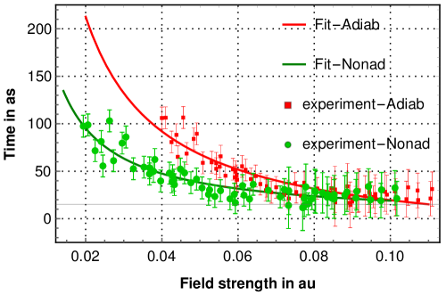
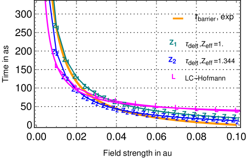
Figure 3: (Color online) Left: tunnel-ionization time-delay versus field strength. Experimental data of adiabatic Landsman et al. (2014) (red) and nonadiabatic Hofmann et al. (2019) (green) field calibrations with their data-fit curves. Right: barrier time-delay $\tau_{barrier,exp}$ (orange) obtained by subtractions of the data-fit curves (shown left), and the barrier time-delay $\tau_{delt}$ of eq. 7 for $Z_{eff}=1,1.344$ (green, blue). As well as the LC-curve (magenta) obtained by data-fit of LC-data given in Hofmann et al. (2019).

This leads us to the interaction time with the laser field in the barrier area, since the LC-time according to Steinberg Steinberg (1995); Spierings and Steinberg (2021) is related to the interaction time within the barrier, which corresponds to the time spent in the barrier or the dwell time $\tau_{dwel}$ Ramos et al. (2020); Büttiker (1983), which in turn equals $\tau_{delt},\tau_{barrier}$ according to the UTTP (and $\tau_{dwel}$ of Winful in eq. 5).

The agreement shown in Fig. 3 (see eq. 8) suggests that the WM value (LC-time) and the interaction time within the barrier region in the thick barrier limit ($\tau_{dwell}$), can be determined by $\tau_{delt}$ ($\approx\tau_{dion}$ of the nonadiabatic field calibration.) We think this is similar to the measurement presented in Ramos et al. (2020) (Measurement of the time spent in the barrier with LC). In addition, the back reaction of the measurement of the system can be found from $\tau_{T,i}$ as the following

$$\lim\limits_{F\ll F_{a}}\tau_{T,i}=\frac{1}{2}\frac{(I_{p}-\delta_{z})}{4Z_{eff}F}=\frac{1}{2}\frac{\varepsilon_{{}_{F}}}{4Z_{eff}F}\approx\frac{2Z_{eff}F}{I_{p}}=\tau_{backr},$$

where $\varepsilon_{F}=I_{p}-\delta_{z}$ is small under the WM condition, it becomes as small as it should be (linear dependence on $F$). The last approximation in this equation result from the expansion of $\delta_{z}=I_{p}\sqrt{1-{4Z_{eff}F}/{I_{p}^{2}}}$ for small $F$.

However, the condition of WM is not necessary and we can assume that $\tau_{T,i}$ always represents the back reaction of the system, which is generally consistent with interpretation as the time needed to reach the barrier entrance in the strong-field interaction, see discussion after eq. 2. Finally, we note that $\tau_{T,d},\tau_{T,i}$ can be interpreted as forward, backward tunneling, respectively Kullie (2015) and a decomposition of $\tau_{T,i}$ similar to eq. 2, $\tau_{T,i}=\tau_{dion}-\tau_{delt}$, shows again that $\tau_{delt}=\tau_{dwell}$, since according to Steinberg Steinberg (1995) we have $\tau_{dwell}=Re(\tau_{T})=Re(\tau_{R})$, where $\tau_{T},\tau_{R}$ are the transmission scattering channel and reflection time respectively Steinberg (1995) and they are forward and backward (tunneling) scattering channels in our model. In our forward, backward channels of adiabatic tunneling in eq. 2, which is illustrated in fig. 2 (dashed-dotted, red curve), the condition of a spatially symmetric barrier noted by Steinberg Steinberg (1995) is reflected by the fact that the horizontal channel happens along the (same) barrier width $d_{B}=x_{e,+}-x_{e,-}$ (or the full width of the barrier) for forward and backward tunneling. Finally we can write $\tau_{T,{d,i}}=\tau_{dion}\pm\tau_{delt}$ and $\tau_{dion}=(1/2)\left(\tau_{T,d}+\tau_{T,i}\right),\tau_{delt}=(1/2)\left(\tau_{T,d}-\tau_{T,i}\right)$, where the symmetrization results in $\tau_{dion}$ and the anti-symmetrization results in the barrier time-delay or the dwell time. For further details and discussion, we would like to refer readers to our previous work Kullie (2020). Forward and backward tunneling is equivalent to the transmission and reflection of the wave packet in the traditional tunneling or quantum tunneling studies, which usually use numerical methods Winful (2003); Lunardi and Manzoni (2019); Dumont and Rivlin (2023); Ma et al. (2024); de Carvalho and Nussenzveig (2002); Winful (2006), whereas our model offers a simple tunneling model with expressions composed of basic laser and atomic parameters that well the measurement result of the attoclock.

Conclusion

The tunneling time shows a universal behavior that we call UTTP, where the barrier time-delay can be defined by $\tau_{delt}\equiv\tau_{barrier}\equiv\tau_{dwell}$. It is shown that $\tau_{delt}$ agrees with the extracted time-delay $\tau_{barrier,exp}$ from the difference between adiabatic and nonadiabatic experimental measurement result of the same experiment. That is the attoclock experiment on He-atom with the adiabatic and nonadiabatic field calibration of Landsman and Hofmann Landsman et al. (2014); Hofmann et al. (2019), respectively. Our result provides conceivable definitions of the tunnel-ionization and barrier time-delays and the interpretation of the attoclock measurement. We also found that the barrier time-delay $\tau_{delt}$ corresponds to the LC-time and the interaction time Büttiker (1983); Steinberg (1995); Ramos et al. (2020); Spierings and Steinberg (2021). This is particularly evident in the limit of thick (opaque) barrier, where $\tau_{delt}$ is close to the time-delay in the nonadiabatic field calibration $\tau_{dion}$, where the back reaction is small and the weak measurement approach is justified. We assume that there is a similarity to the measurement presented in Ramos et al. (2020). In the future, our concern will be devoted to dealing with the superluminal tunnel effect, e.g. Dumont and Rivlin (2023), one of the most exciting and controversial phenomena in quantum physics.

Acknowledgments

I would like to thank Prof. Martin Garcia from the Theoretical Physics of the Institute of Physics at the University of Kassel for his kind support.

References

- Kullie (2015) O. Kullie, Phys. Rev. A 92, 052118 (2015), arXiv:1505.03400v2.
- Augst et al. (1989) S. Augst, D. Strickland, D. D. Meyerhofer, S. L. Chin, and J. H. Eberly, Phys. Rev. Lett. 63, 2212 (1989).
- Augst et al. (1991) S. Augst, D. D. Meyerhofer, D. Strickland, and S. L. Chin, J. Opt. Soc. Am. B 8, 858 (1991).
- Landsman et al. (2014) A. S. Landsman, M. Weger, J. Maurer, R. Boge, A. Ludwig, S. Heuser, C. Cirelli, L. Gallmann, and U. Keller, Optica 1, 343 (2014).
- Delone and Kraǐnov (1998) N. B. Delone and V. P. Kraǐnov, Phys.-Usp. 41, 469 (1998).
- Kiyan and Kraǐnov (1991) I. Y. Kiyan and V. P. Kraǐnov, Soviet Phys. JETP 73, 429 (1991).
- Kullie (2016) O. Kullie, Journal of Physics B: Atomic, Molecular and Optical Physics 49, 095601 (2016).
- Kullie (2018) O. Kullie, Ann. of Phys. 389, 333 (2018), arXiv:1701.05012.
- Kullie (2020) O. Kullie, Qunat. Rep. 2, 233 (2020).
- Hofmann et al. (2019) C. Hofmann, A. S. Landsman, and U. Keller, J. Mod. Opt. 66, 1052 (2019).
- Kullie (2024) O. Kullie, Ann. of Phys. (2024), 10.2139/ssrn.4707729, under Review.
- Winful (2003) H. G. Winful, Phys. Rev. Lett. 91, 260401 (2003).
- Lunardi and Manzoni (2019) J. T. Lunardi and L. A. Manzoni, J. Phys.: Conference Series 1391, 012112 (2019).
- Lunardi and Manzoni (2018) J. T. Lunardi and L. A. Manzoni, Advances in High Energy Physics 2018, ”ID1372359” (2018).
- Hartman (1962) T. E. Hartman, J. Appl. Phys. 33, 3427 (1962).
- Eckle et al. (2008a) P. Eckle, M. Smolarski, F. Schlup, J. Biegert, A. Staudte, M. Schöffler, H. G. Muller, R. Dörner, and U. Keller, Nat. Phys. 4, 565 (2008a).
- Eckle et al. (2008b) P. Eckle, A. N. Pfeiffer, C. Cirelli, A. Staudte, R. Dörner, H. G. Muller, M. Büttiker, and U. Keller, Sience 322, 1525 (2008b).
- Aharonov et al. (1988) Y. Aharonov, D. Z. Albert, and L. Vaidman, Phys. Rev. Lett. 60, 1351 (1988).
- Rozema et al. (2012) L. A. Rozema, A. Darabi, D. H. Mahler, A. Hayat, Y. Soudagar, and A. M. Steinberg, Phys. Rev. Lett. 109, 100404 (2012).
- Landsman and Keller (2015) A. S. Landsman and U. Keller, Phys. Rep. 547, 1 (2015).
- Steinberg (1995) A. M. Steinberg, Phys. Rev. Lett. 74, 2405 (1995).
- Spierings and Steinberg (2021) D. C. Spierings and A. M. Steinberg, Phys. Rev. Lett. 127, 133001 (2021).
- Ramos et al. (2020) R. Ramos, D. Spierings, I. Racicot, and A. M. Steinberg, Nature 583, 529 (2020).
- Büttiker (1983) M. Büttiker, Phys. Rev. B 27, 6178 (1983).
- Dumont and Rivlin (2023) R. S. Dumont and T. Rivlin, Phys. Rev. A 107, 052212 (2023).
- Ma et al. (2024) Y. Ma, H. Ni, and J. Wu, Chinese Physics B 33, 013201 (2024).
- de Carvalho and Nussenzveig (2002) C. A. A. de Carvalho and H. M. Nussenzveig, Phys. Rep. 364, 83 (2002).
- Winful (2006) H. G. Winful, Phys. Rep. 436, 1 (2006).