Spatially sparse optimization problems in fractional order Sobolev spaces

Abstract

We investigate time-dependent optimization problems in fractional Sobolev spaces with the sparsity promoting $L^{p}$-pseudo norm for $0<p<1$ in the objective functional. In order to avoid computing the fractional Laplacian on the time-space cylinder $I\times\Omega$, we introduce an auxiliary function $w$ on $\Omega$ that is an upper bound for the function $u\in L^{2}(I\times\Omega)$. We prove existence and regularity results and derive a necessary optimality condition. This is done by smoothing the $L^{p}$-pseudo norm and by penalizing the inequality constraint regarding $u$ and $w$. The problem is solved numerically with an iterative scheme whose weak limit points satisfy a weaker form of the necessary optimality condition.

49K30, 49M20

1 Introduction

The aim of this paper is to investigate spatially sparse time dependent optimization problems in fractional order Sobolev spaces. A first general formulation of such a minimization problem is

$$\underset{u\in H^{s}(I\times\Omega)}{\min}f(u)+\frac{\alpha}{2}\|u\|_{H^{s}(I\times\Omega)}^{2}+\int_{\Omega}\left(\int_{I}|u(t,x)|^{2}\mathop{}\!\mathrm{d}t\right)^{p}\mathop{}\!\mathrm{d}x.$$ (1)

Here, $\Omega\subset\mathbb{R}^{d}$ denotes a Lipschitz domain, $I$ some time interval and $f:L^{2}(I\times\Omega)\to\mathbb{R}$ is some smooth enough function. In the context of optimal control, this would be the state dependent part of an optimal control problem.

The motivation for considering such minimization problems arises from sparse optimal control problems where the aim is to find controls with small support. Applications for this are for example actuator placement problems. There is a variety of sparsity promoting terms that can be added to the objective to force solutions to be sparse. A widely used example is the $L^{1}$-norm as introduced in [85l1Sparse]. Another non-smooth and additionally also non-convex possibility that we employ here is the $L^{p}$-pseudo norm

$$\|w\|_{p}^{p}\coloneqq\int_{\Omega}|w|^{p}\mathop{}\!\mathrm{d}x$$

for $p\in(0,1)$. This approach was also investigated in [lp_cont]. For $p=0$, the $L^{0}$-functional measures the support of a function. This was for example discussed in [lp_cont, l0optimalControl].

For time and space dependent functions, different sparsity patterns are investigated in [80dirSparse]. In [81spatTempSparse], the concept of directional sparsity is introduced, where the spatial domain on which a function is sparse for all times is considered.

The formulation involving the $L^{p}$-pseudo norm in the last term of (1) leads to directionally sparse solutions $u$, i.e. the spatial domain on which the solution vanishes on the whole time interval $I$ tends to be large.

The reason to work in the fractional Sobolev space $H^{s}(I\times\Omega)$ is to ensure existence of solutions of the minimization problem (1): If the problem was set in $L^{2}(I\times\Omega)$ instead, it was shown in [lp_cont] that it is impossible to guarantee the existence of minimizers. This is a consequence of the $L^{p}$-pseudonorm not being weakly lower semicontinuous. However, thanks to the compact embedding $H^{s}(I\times\Omega)\hookrightarrow L^{2}(I\times\Omega)$, the map ${u\mapsto\int_{\Omega}\left(\int_{I}|u(t,x)|^{2}\mathop{}\!\mathrm{d}t\right)^{p}\mathop{}\!\mathrm{d}x}$ is weakly continuous and we can therefore pass to the weak limit in a minimizing sequence and the standard proof for existence of solutions works. We choose the fractional Sobolev space $H^{s}$ for $s\in(0,1)$ and not the standard Sobolev space $H^{1}$ to avoid requiring too much smoothness. Particularly, for $s<\frac{1}{2}$, fractional Sobolev spaces also contain discontinuous functions. Regularization with the $H^{s}(\Omega)$-norm has for example applications in image denoising or phase-field models as shown in [83applic].

When solving problem (1) numerically one needs to solve equations involving the fractional Laplacian on the $(d+1)$-dimensional domain $I\times\Omega$, which is computationally expensive. Therefore, we introduce an auxiliary function $w$ defined only on the spatial domain $\Omega$ and rewrite the problem as

$$\underset{u\in L^{2}(I\times\Omega),w\in H^{s}(\Omega)}{\min}f(u)+\frac{\alpha}{2}\|u\|_{L^{2}(I\times\Omega)}^{2}+\frac{\beta}{2}\|w\|_{H^{s}(\Omega)}^{2}+\gamma\|w\|_{p}^{p}$$ (2)

subject to

$$|u(t,x)|\leq w(x)\hskip 14.22636pt\textrm{a.a.}(t,x)\in I\times\Omega$$ (3)

with $\alpha,\beta,\gamma>0$. With this construction we only need to solve equations involving the fractional Laplacian on $\Omega$. At the same time, it is still possible to prove existence of solutions by standard methods and we still obtain spatially sparse solutions $u$ due to the constraint that couples the two function $u$ and $w$. This paper is a generalization to the time-dependent case of [sparse]. Analogous to that paper, we prove an optimality condition for solutions of (2) by using a smoothing scheme introduced in [lp_cont] to deal with the non-smooth $L^{p}$-pseudonorm. With this scheme we obtain a smooth approximation of the $L^{p}$-term. However, this approximation is not concave anymore. Other approximation approaches like a Huber type regularization presented in [87huberApprox] for example lead to non-smooth but concave approximations. The smooth approximation leads to an auxiliary problem depending on a smoothing parameter $\epsilon>0$. For this auxiliary problem it is now possible to obtain an optimality condition, and our aim is to derive an optimality condition of the original problem by passing to the limit $\epsilon\searrow 0$ as done in [sparse]. In order to do that, we also penalize the constraint (3) to obtain boundedness of all the quantities involved in the optimality condition of the auxiliary problem. This step is not necessary in [sparse], where the optimization problem is unconstrained.

The structure of the paper is as follows. First, we give a brief overview of fractional Sobolev spaces in Section 2. Then, we prove existence of solutions of the minimization problem in Section 3 and derive an auxiliary problem with a smoothing and penalization scheme in the subsequent Section 4. This auxiliary problem is used in Section 4.1 to obtain an optimality condition for the minimization problem (2). In Section 5 we consider an iterative scheme to solve this minimization problem. We conclude by giving some numerical examples in Section 6.

Notation

Throughout this paper, $\Omega\subset\mathbb{R}^{d}$ denotes a Lipschitz domain and $I=[0,T]$ some time interval with $T>0$. Furthermore, we use the abbreviation $U\coloneqq L^{2}(I\times\Omega)$. The space $W$ will be defined below as a suitable fractional Sobolev space on $\Omega$. We denote by

$$K\coloneqq\{(u,w)\in U\times W:\ |u(t,x)|\leq w(x)\textrm{ for a.a. }(t,x)\in I\times\Omega\}$$ (4)

the set of admissible functions. Moreover, we use the notation $(\cdot,\cdot)_{V}$ for the inner product of a Hilbert space $V$ and $\braket{\cdot,\cdot}_{V}$ for its duality product. We use the notation $(u)_{-}$ and $(u)_{+}$ to describe the negative or positive part of a function $u$.

When we use a function $w$ defined on the spatial domain $\Omega$ in an expression involving the time-space cylinder $I\times\Omega$, we employ the constant extension of $w$ from $\Omega$ to $I\times\Omega$ with $w(t,x)\coloneqq w(x)$ for (almost all) $(t,x)\in\times\Omega$.

2 Fractional Sobolev spaces

In this section, we state some definitions and results about fractional order Sobolev spaces.

Definition 2.1.

Let $s\in(0,1)$. Then, the fractional order Sobolev space $H^{s}(\Omega)$ is defined as

$$H^{s}(\Omega)\coloneqq\left\{w\in L^{2}(\Omega):\ (x,y)\mapsto\frac{|w(x)-w(y)|}{|x-y|^{\frac{d}{2}+s}}\in L^{2}(\Omega\times\Omega)\right\}$$

with the corresponding norm

$$\|w\|_{H^{s}(\Omega)}\coloneqq\left(\int_{\Omega}|w|^{2}\mathop{}\!\mathrm{d}x+\frac{c_{d,s}}{2}\int_{\Omega}\int_{\Omega}\frac{|w(x)-w(y)|^{2}}{|x-y|^{d+2s}}\mathop{}\!\mathrm{d}x\mathop{}\!\mathrm{d}y\right)^{\frac{1}{2}}$$

and $c_{d,s}\coloneqq\frac{s2^{2s}\Gamma(s+\frac{d}{2})}{\pi^{\frac{d}{2}}\Gamma(1-s)}.$

With this norm, one can define the space $H_{0}^{s}(\Omega)$ as

$$H_{0}^{s}(\Omega)\coloneqq\overline{C_{c}^{\infty}(\Omega)}^{H^{s}(\Omega)},$$

where $C_{c}^{\infty}(\Omega)$ is the space of infinitely continuously differentiable functions with compact support in $\Omega$. Moreover, let

$$\tilde{H}^{s}(\Omega)\coloneqq\left\{w\in H^{s}(\mathbb{R}^{d}):w_{|\mathbb{R}^{d}\setminus\Omega}=0\right\}=\overline{C_{c}^{\infty}(\Omega)}^{H^{s}(\mathbb{R}^{d})}.$$

For $s=\frac{1}{2}$, the Lions-Magenes space is defined as

$$H_{00}^{\frac{1}{2}}(\Omega)\coloneqq\left\{w\in L^{2}(\Omega):\int_{\Omega}\frac{w^{2}(x)}{\operatorname{dist}(x,\partial\Omega)}\mathop{}\!\mathrm{d}x<\infty\right\}$$

with the norm

$$\|w\|_{H_{00}^{\frac{1}{2}}(\Omega)}\coloneqq\left(\|w\|^{2}_{H^{\frac{1}{2}}(\Omega)}+\int_{\Omega}\frac{w^{2}(x)}{\operatorname{dist}(x,\partial\Omega)}\mathop{}\!\mathrm{d}x\right)^{\frac{1}{2}}.$$

For this space it holds $H_{00}^{\frac{1}{2}}(\Omega)\subsetneq H^{\frac{1}{2}}(\Omega)$.

Another way to define fractional Sobolev spaces is via spectral theory using eigenvectors and eigenfunctions of the Laplace operator with Dirichlet boundary conditions $\Delta_{D}$.

Definition 2.2.

Let $s\geq 0$. Then, the fractional order Sobolev space in spectral form is defined as

$$\mathbb{H}^{s}(\Omega)\coloneqq\left\{w=\sum_{n=1}^{\infty}w_{n}\phi_{n}\in L^{2}(\Omega):\|w\|_{\mathbb{H}^{s}}^{2}\coloneqq\sum_{n=1}^{\infty}\lambda_{n}^{s}w_{n}^{2}<\infty\right\},$$

where $w_{n}\coloneqq\int_{\Omega}w\phi_{n}\mathop{}\!\mathrm{d}x$, and $\phi_{n}$ are the eigenfunctions of the Laplacian with Dirichlet boundary conditions to the eigenvalues $\lambda_{n}$.

One can also rewrite this norm in an integral formulation as done in [nonhomBC, anote], namely

$$\|w\|^{2}_{\mathbb{H}^{s}(\Omega)}=\frac{1}{2}\int_{\Omega}\int_{\Omega}|(w(x)-w(y))|^{2}J(x,y)\mathop{}\!\mathrm{d}y\mathop{}\!\mathrm{d}x+\int_{\Omega}\kappa(x)|w(x)|^{2}\mathop{}\!\mathrm{d}x.$$ (5)

Here, the function $J$ is given by

$$J(x,y)=\frac{s}{\Gamma(1-s)}\int_{0}^{\infty}\frac{K_{\Omega}(t,x,y)}{t^{1+s}}\mathop{}\!\mathrm{d}t,$$

with $K_{\Omega}$ being the heat kernel of the semigroup generated by the operator $-\Delta_{D}$ on $L^{2}(\Omega)$. The function $\kappa$ is given by

$$\kappa(x)=\frac{s}{\Gamma(1-s)}\int_{0}^{\infty}\left(1-\int_{\Omega}K_{\Omega}(t,x,y)\mathop{}\!\mathrm{d}y\right)\frac{\mathop{}\!\mathrm{d}t}{t^{1+s}}.$$

Note that $\kappa$ and $J$ are both non-negative and $J$ is symmetric with $J(x,y)=J(y,x)$ for a.a. $x,y\in\Omega$.

It was shown in [105ellipticProb, lions] that we have the equalities

$$\mathbb{H}^{s}(\Omega)=\begin{cases}H^{s}(\Omega)=H_{0}^{s}(\Omega)=\tilde{H}^{s}(\Omega)&\textrm{ if }0<s<\frac{1}{2},\\ H_{00}^{1/2}(\Omega)&\textrm{ if }s=\frac{1}{2},\\ H_{0}^{s}(\Omega)=\tilde{H}^{s}(\Omega)&\textrm{ if }\frac{1}{2}<s<1,\end{cases}$$ (6)

with equivalence of norms. From now on, the space $W$ refers to a fractional Sobolev space that is covered by the previous result, i.e.,

$$W\in\{\ H^{s}(\Omega),\ H_{0}^{s}(\Omega),\ \tilde{H}^{s}(\Omega),\ \mathbb{H}^{s}(\Omega)\ \}$$

for some $s\in(0,1)$.

The following properties of these fractional Sobolev spaces will be used later on.

Lemma 2.3.

1. The embedding $W\hookrightarrow L^{2}(\Omega)$ is compact.

2. Let $w\in W$ and let $z(x)\coloneqq\max(-1,\min(w(x),1))$. Then, $z\in W$ and $\braket{w,z}_{W}\geq\|z\|_{W}^{2}$.

3. $C_{0}(\Omega)\cap W$ is dense in $W$ and $C_{0}(\Omega)$.

4. There is $q>2$ such that $W$ is continuously embedded in $L^{q}(\Omega)$. More precisely,

   $$W\hookrightarrow\begin{cases}L^{\frac{2d}{d-2s}}(\Omega)&\textrm{if }d>2s,\\ L^{p}(\Omega)\quad\forall p\in[1,\infty)&\textrm{if }d=2s,\\ C^{0,s-\frac{d}{2}}(\bar{\Omega})&\textrm{if }d<2s.\end{cases}$$

Proof.

This is shown in [sparse, Section 6] and [hitch, Sections 6, 7]. ∎

Lemma 2.4.

Let $w\in W$ and $w^{+}\coloneqq\max(w,0)$. Then $(w,w^{+})_{W}\leq\|w\|_{W}^{2}$.

Proof.

One can directly see that the inequality holds for the $L^{2}(\Omega)$-part in the $W$-norm. Furthermore, it holds a.e.

$$(w^{+}(x)-w^{+}(y))\cdot(w(x)-w(y))\leq(w(x)-w(y))^{2}.$$

This can be seen by considering the following cases:

1. If $w(x)\geq 0$ and $w(y)\geq 0$, it holds $(w^{+}(x)-w^{+}(y))\cdot(w(x)-w(y))=(w(x)-w(y))^{2}.$

2. For $w(x)\leq 0$ and $w(y)\leq 0$ we get $(w^{+}(x)-w^{+}(y))\cdot(w(x)-w(y))=0\leq(w(x)-w(y))^{2}.$

3. If $w(x)\geq 0$ and $w(y)\leq 0$, it holds $(w^{+}(x)-w^{+}(y))\cdot(w(x)-w(y))=(w^{+}(x))\cdot(w(x)-w(y))\leq(w(x)-w(y))^{2}.$

4. Similarly, for $w(x)\leq 0$ and $w(y)\geq 0$ we obtain $(w^{+}(x)-w^{+}(y))\cdot(w(x)-w(y))=(-w^{+}(y))\cdot(w(x)-w(y))\leq(w(x)-w(y))^{2}.$

By definition of the inner product in $W$ this yields the result for $H_{0}^{s}(\Omega)$, $\tilde{H}^{s}(\Omega)$ and also for the spectral fractional Sobolev space $\mathbb{H}^{s}(\Omega)$ using its integral formulation (5). It can be easily seen that the additional term appearing in the case $H_{00}^{\frac{1}{2}}(\Omega)$ also satisfies the inequality. ∎

3 Existence of Solutions

We now want to prove existence of solutions of the above introduced minimization problem

$$\underset{(u,w)\in K}{\min}f(u)+\frac{\alpha}{2}\|u\|_{U}^{2}+\frac{\beta}{2}\|w\|_{W}^{2}+\gamma\int_{\Omega}|w|^{p}\mathop{}\!\mathrm{d}x.$$

Note that the set $K$ of admissible functions defined in (4) is convex. First, we state some assumptions that should hold throughout the paper.

Assumption 3.1.

1. The function $f\colon U\to\mathbb{R}$ is weakly lower semicontinuous and bounded from below by an affine function, i.e., there are $g\in U^{*}$, $c\in\mathbb{R}$ such that $f(u)\geq g(u)+c$ for all $u\in U$.

2. Furthermore, $f\colon U\to\mathbb{R}$ is continuously Fréchet differentiable.

3. The constants $\alpha$, $\beta$, $\gamma$ are positive, and $p\in(0,1)$.

Theorem 3.2.

Under Assumption (3.1), the minimization problem (2) admits a solution.

Proof.

This statement can be shown with standard arguments. Let $(u_{n},w_{n})$ be a minimizing sequence. Then, Assumption 3.1 yields boundedness of $(u_{n})$ in $U$ and $(w_{n})$ in $W$, respectively. Hence, there are $\bar{u}\in U$ and $\bar{w}\in W$ such that $u_{n}\rightharpoonup\bar{u}$ in $U$ and $w_{n}\rightharpoonup\bar{w}$ in $W$ with $w_{n}\to\bar{w}$ in $L^{2}(\Omega)$. This implies $\gamma\int_{\Omega}|w_{n}|^{p}\mathop{}\!\mathrm{d}x\to\gamma\int_{\Omega}|\bar{w}|^{p}\mathop{}\!\mathrm{d}x$, see [lp_cont]. Since $K$ is closed and convex and therefore weakly closed, it holds $(\bar{u},\bar{w})\in K$. Thus,

$$\liminf_{n\to\infty}f(u_{n})+\frac{\alpha}{2}\|u_{n}\|_{U}^{2}+\frac{\beta}{2}\|w_{n}\|_{W}^{2}+\gamma\int_{\Omega}|w_{n}|^{p}\mathop{}\!\mathrm{d}x$$

$$\geq f(\bar{u})+\frac{\alpha}{2}\|\bar{u}\|_{U}^{2}+\frac{\beta}{2}\|\bar{w}\|_{W}^{2}+\gamma\int_{\Omega}|\bar{w}|^{p}\mathop{}\!\mathrm{d}x$$

due to weak lower semicontinuity. This shows that $(\bar{u},\bar{w})$ realizes the minimum. ∎

4 Auxiliary problem with smoothing and penalization scheme

The next step is to derive a sequence of auxiliary minimization problems that are smooth enough to directly obtain necessary optimality conditions. These optimality conditions can then be used to derive an optimality condition for the original problem (2).

To do so, we use a smoothing scheme as in [sparse, lp_cont]. There, a smooth approximation of $t\mapsto t^{p/2}$ is introduced by

$$\psi_{\epsilon}(t)\coloneqq\begin{cases}\frac{p}{2}\frac{t}{\epsilon^{2-p}}+(1-\frac{p}{2})\epsilon^{p}&\textrm{if }t\in[0,\epsilon^{2}),\\ t^{p/2}&\textrm{if }t\geq\epsilon^{2}\end{cases}$$

with derivative

$$\psi_{\epsilon}^{\prime}(t)=\frac{p}{2}\min(\epsilon^{p-2},t^{\frac{p-2}{2}}).$$

Then,

$$G_{\epsilon}(w)\coloneqq\int_{\Omega}\psi_{\epsilon}(|w|^{2})\mathop{}\!\mathrm{d}x$$

is an approximation of $\int_{\Omega}|w|^{p}\mathop{}\!\mathrm{d}x$. For the convergence analysis later on we use the following results of [sparse].

Lemma 4.1.

([sparse, Lemma 4.1, 4.2, 4.3]) Let $p\in(0,2)$. Then $\psi_{\epsilon}:[0,\infty)\to[0,\infty)$ has the following properties:

1. The function $\psi_{\epsilon}$ is concave.

2. $\epsilon\mapsto\psi_{\epsilon}(t)$ is monotonically increasing for all $t\geq 0$.

3. For sequences $(w_{k})$, $(\epsilon_{k})$ such that $w_{k}\to w$ in $L^{1}(\Omega)$ and $\epsilon_{k}\to\epsilon\geq 0$ it holds $G_{\epsilon_{k}}(w_{k})\to G_{\epsilon}(w)$.

4. Let $\epsilon>0$. Then $\psi$ is continuously differentiable with $0\leq\psi_{\epsilon}^{\prime}\leq\frac{p}{2}\epsilon^{p-2}$, and $u\mapsto G_{\epsilon}(u)$ is Fréchet differentiable from $L^{2}(\Omega)$ to $\mathbb{R}$ with

   $$G_{\epsilon}^{\prime}(u)h=\int_{\Omega}2u(x)\psi_{\epsilon}^{\prime}(u(x)^{2})h(x)\mathop{}\!\mathrm{d}x.$$

We remark that while $\psi_{\epsilon}$ is concave, this is not the case for the composition $t\mapsto\psi_{\epsilon}(t^{2})$ that we use in the definition of $G$ to approximate the $L^{p}$-pseudonorm.
Now we can replace the $L^{p}$-pseudo norm by its smooth approximation to obtain the auxiliary objective function

$$\Phi_{\epsilon}(u,w)=f(u)+\frac{\alpha}{2}\|u\|_{U}^{2}+\frac{\beta}{2}\|w\|_{W}^{2}+\gamma G_{\epsilon}(w).$$ (7)

Next, we also penalize the violation of the constraint $|u|\leq w$ in the original minimization problem. This enables us to obtain boundedness of the terms corresponding to the smoothing scheme in the auxiliary optimality condition when passing to the limit $\epsilon\to 0$ later on. Therefore, we rewrite problem (2) as

$$\underset{u\in U,w\in W}{\min}\Phi_{\epsilon}(u,w)+\frac{1}{2\epsilon}\|(w-u)_{-}\|_{U}^{2}+\frac{1}{2\epsilon}\|(w+u)_{-}\|_{U}^{2}.$$

In this problem, the $L^{2}(I\times\Omega)$-norm of the parts that violate the constraint are added and multiplied with a penalization parameter $\frac{1}{\epsilon}$. Here, we used the notation

$$\|(w-u)_{-}\|_{U}^{2}:=\int_{\Omega}\int_{I}(w(x)-u(t,x))_{-}^{2}\mathop{}\!\mathrm{d}t\mathop{}\!\mathrm{d}x,$$

and similarly for $\|(w+u)_{-}\|_{U}^{2}$, so that we used a constant extension of $w$ from $\Omega$ to $I\times\Omega$. Note that this penalization is an additional step compared to the procedure in [sparse], where the considered minimization problem is unconstrained.

Let $(\bar{u},\bar{w})$ be a local solution of the non-smooth problem (2). Then there is $\rho>0$ such that $\Phi_{0}(\bar{u},\bar{w})\leq\Phi_{0}(u,w)$ for all $(u,w)$ with $\|u-\bar{u}\|_{U}\leq\rho,\|w-\bar{w}\|_{W}\leq\rho$ and $(u,w)\in K$. The corresponding auxiliary problem

$$\begin{gathered}\underset{u\in U,w\in W}{\min}\Phi_{\epsilon}(u,w)+\frac{1}{2}\|u-\bar{u}\|^{2}_{U}+\frac{1}{2}\|w-\bar{w}\|_{L^{2}(\Omega)}^{2}+\frac{1}{2\epsilon}\|(w-u)_{-}\|_{U}^{2}+\frac{1}{2\epsilon}\|(w+u)_{-}\|_{U}^{2}\\ \textrm{s.t. }\|u-\bar{u}\|_{U}\leq\rho,\|w-\bar{w}\|_{W}\leq\rho\end{gathered}$$ (8)

has a solution according to standard arguments similarly as in Theorem 3.2.

4.1 Optimality conditions

In order to derive an optimality condition for problem (2), we pass to the limit $\epsilon\searrow 0$ in the optimality condition of problem (8). But first, we show that solutions of (8) converge to the reference solution for $\epsilon\searrow 0$. We start with an auxiliary lemma.

Lemma 4.2.

Let $N\in\mathbb{N}$. Let $(a^{1}_{k}),\dots,(a^{N}_{k})$ be sequences with

$$\liminf_{k\to\infty}a_{k}^{i}\in\mathbb{R}\quad\forall i=1,\dots,N$$

and

$$\limsup_{k\to\infty}\left(\sum_{i=1}^{N}a^{i}_{k}\right)=\sum_{i=1}^{N}(\liminf_{k\to\infty}a^{i}_{k}).$$

Then all sequences $(a^{1}_{k}),...,(a^{N}_{k})$ are convergent with limits in $\mathbb{R}$.

Proof.

The claim is elementary for $N=1$. Let the claim be proven for some $N\geq 1$. Consider $N+1$ sequences satisfying the assumptions of the lemma. Then

$$\limsup_{k\to\infty}\left(\sum_{i=1}^{N}a^{i}_{k}\right)+\liminf_{k\to\infty}a^{N+1}_{k}\leq\limsup_{k\to\infty}\left(\sum_{i=1}^{N+1}a^{i}_{k}\right)\leq\sum_{i=1}^{N+1}(\liminf_{k\to\infty}a^{i}_{k}).$$

This implies $\limsup_{k\to\infty}\left(\sum_{i=1}^{N}a^{i}_{k}\right)=\sum_{i=1}^{N}(\liminf_{k\to\infty}a^{i}_{k})$, and hence the sequences $(a^{1}_{k}),...,(a^{N}_{k})$ converge by induction hypothesis. We obtain $\limsup_{k\to\infty}a^{N+1}_{k}\leq\liminf_{k\to\infty}a^{N+1}_{k}$, and $(a^{N+1}_{k})$ converges as well.

∎

Lemma 4.3.

Let $\epsilon_{k}\searrow 0$ and let $(u_{k},w_{k})$ be the solution of (8) for the corresponding smoothing parameter $\epsilon_{k}$. Suppose $u_{k}\rightharpoonup u^{*}$ in $U$, $w_{k}\rightharpoonup w^{*}$ in $W$, and

$$\Phi_{0}(u^{*},w^{*})\geq\limsup_{k\to\infty}\Phi_{\epsilon_{k}}(u_{k},w_{k}).$$

Then $u_{k}\to u^{*}$ in $U$ and $w_{k}\to w^{*}$ in $W$.

Proof.

We want to apply Lemma 4.2 to the terms in $\Phi_{\epsilon_{k}}(u_{k},w_{k})$. By Lemma 4.1 (iii), it holds ${G_{\epsilon_{k}}(w_{k})\to G_{0}(w^{*})}$, which implies

$$\liminf_{k\to\infty}\Phi_{\epsilon_{k}}(u_{k},w_{k})\\ \begin{aligned} &\geq\liminf_{k\to\infty}f(u_{k})+\liminf_{k\to\infty}\frac{\alpha}{2}\|u_{k}\|_{U}^{2}+\liminf_{k\to\infty}\frac{\beta}{2}\|w_{k}\|_{W}^{2}+\liminf_{k\to\infty}\gamma G_{\epsilon}(w_{k})\\ &\geq\Phi_{0}(u^{*},w^{*})\end{aligned}$$

by weak lower semicontinuity of $f$. Together with the assumption, this yields

$$\liminf_{k\to\infty}f(u_{k})+\liminf_{k\to\infty}\frac{\alpha}{2}\|u_{k}\|_{U}^{2}+\liminf_{k\to\infty}\frac{\beta}{2}\|w_{k}\|_{W}^{2}+\liminf_{k\to\infty}\gamma G_{\epsilon}(w_{k})=\limsup_{k\to\infty}\Phi_{\epsilon_{k}}(u_{k},w_{k}),$$

and the assumptions of Lemma 4.2 are satisfied. Therefore, we obtain convergence of all the terms in $\Phi_{\epsilon_{k}}(u_{k},w_{k})$. In particular, it holds $\|u_{k}\|_{U}\to\|u^{*}\|_{U}$ and $\|w_{k}\|_{W}\to\|w^{*}\|_{W}$ which together with weak convergence of $(u_{k})$ and $(w_{k})$ leads to the desired result. ∎

Theorem 4.4.

Let $\epsilon_{k}\searrow 0$, and let $(u_{k},w_{k})$ be solutions of (8) for the corresponding smoothing parameter $\epsilon_{k}$. Then, $u_{k}\to\bar{u}$ in $U$ and $w_{k}\to\bar{w}$ in $W$.

Proof.

The sequences $(u_{k})$ and $(w_{k})$ are bounded in $U$ and $W$, respectively, due to the constraints in (8). Hence, there are $u^{*}\in U$, $w^{*}\in W$ such that (after extracting a subsequence if necessary) $u_{k}\rightharpoonup u^{*}$ in $U$, $w_{k}\rightharpoonup w^{*}$ in $W$, and $w_{k}\to w^{*}$ in $L^{2}(\Omega)$. Using Lemma 4.1 (iii), it holds $G_{\epsilon_{k}}(\bar{w})\to G_{0}(\bar{w})$, so that $\Phi_{\epsilon_{k}}(\bar{u},\bar{w})\to\Phi_{0}(\bar{u},\bar{w})$ follows. From optimality of $(u_{k},w_{k})$ in (8) we get

$$\Phi_{\epsilon_{k}}(\bar{u},\bar{w})\geq\Phi_{\epsilon_{k}}(u_{k},w_{k})+\frac{1}{2}\|u_{k}-\bar{u}\|^{2}_{U}+\frac{1}{2}\|w_{k}-\bar{w}\|_{L^{2}(\Omega)}^{2}\\ +\frac{1}{2\epsilon_{k}}\|(w_{k}-u_{k})_{-}\|_{U}^{2}+\frac{1}{2\epsilon_{k}}\|(w_{k}+u_{k})_{-}\|_{U}^{2}.$$ (9)

Passing to the limit superior leads to

$$\Phi_{0}(\bar{u},\bar{w}) \geq\limsup_{k\to\infty}\left(\Phi_{\epsilon_{k}}(u_{k},w_{k})+\frac{1}{2}\|u_{k}-\bar{u}\|^{2}_{U}+\frac{1}{2}\|w_{k}-\bar{w}\|_{L^{2}(\Omega)}^{2}\right.$$

$$\quad+\left.\frac{1}{2\epsilon_{k}}\|(w_{k}-u_{k})_{-}\|_{U}^{2}+\frac{1}{2\epsilon_{k}}\|(w_{k}+u_{k})_{-}\|_{U}^{2}\right)$$

$$\geq\liminf_{k\to\infty}\Phi_{\epsilon_{k}}(u_{k},w_{k})+\liminf_{k\to\infty}\frac{1}{2}\|u_{k}-\bar{u}\|^{2}_{U}+\liminf_{k\to\infty}\frac{1}{2}\|w_{k}-\bar{w}\|_{L^{2}(\Omega)}^{2}$$

$$\quad+\liminf_{k\to\infty}\frac{1}{2\epsilon_{k}}\|(w_{k}-u_{k})_{-}\|_{U}^{2}+\liminf_{k\to\infty}\frac{1}{2\epsilon_{k}}\|(w_{k}+u_{k})_{-}\|_{U}^{2}$$

$$\geq\Phi_{0}(u^{*},w^{*})+\frac{1}{2}\|u^{*}-\bar{u}\|^{2}_{U}+\frac{1}{2}\|w^{*}-\bar{w}\|_{L^{2}(\Omega)}^{2}.$$

From these inequalities we obtain boundedness of the terms $\frac{1}{2\epsilon_{k}}\|(w_{k}\pm u_{k})_{-}\|_{U}^{2}$. Since $\epsilon_{k}\to 0$, it holds $\|(w_{k}\pm u_{k})_{-}\|_{U}\to 0$. By definition, we have $w_{k}-u_{k}-(w_{k}-u_{k})_{-}\in\{v\in U:v\geq 0\textrm{ a.e. }\}$. This set is weakly closed. Using $w_{k}-u_{k}\rightharpoonup w^{*}-u^{*}$ in $U$ and $(w_{k}-u_{k})_{-}\to 0$ in $U$, it follows $w^{*}-u^{*}\geq 0$ almost everywhere on $I\times\Omega$. Similarly, one can show $u^{*}\geq-w^{*}$ almost everywhere, and therefore $(u^{*},w^{*})$ is admissible for (8). By optimality of $(\bar{u},\bar{w})$ we get together with the chain of inequalities above

$$\Phi_{0}(\bar{u},\bar{w})\geq\Phi_{0}(u^{*},w^{*})+\frac{1}{2}\|u^{*}-\bar{u}\|^{2}_{U}+\frac{1}{2}\|w^{*}-\bar{w}\|_{L^{2}(\Omega)}^{2}\geq\Phi_{0}(\bar{u},\bar{w}),$$

which implies that $(\bar{u},\bar{w})=(u^{*},w^{*})$. The chain of inequalities above also gives $\Phi_{0}(\bar{u},\bar{w})\geq\limsup_{k\to\infty}\Phi_{\epsilon_{k}}(u_{k},w_{k})$, which together with Lemma 4.3 yields strong convergence $u_{k}\to\bar{u}$ in $U$ and $w_{k}\to\bar{w}$ in $W$. ∎

Next, we consider a necessary optimality condition for problem (8).

Lemma 4.5.

For some $\epsilon>0$, let $(u_{\epsilon},w_{\epsilon})$ be a solution of (8) with $\|u_{\epsilon}-\bar{u}\|_{U}<\rho$ and $\|w_{\epsilon}-\bar{w}\|_{W}<\rho$. Then it holds

$$\begin{gathered}f^{\prime}(u_{\epsilon})v+\alpha(u_{\epsilon},v)_{U}+\beta(w_{\epsilon},z)_{W}+\gamma G_{\epsilon}^{\prime}(w_{\epsilon})z+(u_{\epsilon}-\bar{u},v)_{U}+(w_{\epsilon}-\bar{w},z)_{L^{2}(\Omega)}\\ +\frac{1}{\epsilon}((w_{\epsilon}-u_{\epsilon})_{-},\ z-v)_{U}+\frac{1}{\epsilon}((w_{\epsilon}+u_{\epsilon})_{-},\ z+v)_{U}=0\ \forall(v,z)\in U\times W.\end{gathered}$$ (10)

Here, we used the notation

$$((w_{\epsilon}\pm u_{\epsilon})_{-},\ z\pm v)_{U}:=\int_{\Omega}\int_{I}(w_{\epsilon}(x)\pm u_{\epsilon}(t,x))_{-}\cdot(z(x)\pm v(t,x))\mathop{}\!\mathrm{d}t\mathop{}\!\mathrm{d}x.$$

Proof.

Since the objective function of problem (8) is directionally differentiable, a necessary optimality condition is

$$f^{\prime}(u_{\epsilon})(v-u_{\epsilon})+\alpha(u_{\epsilon},v-u_{\epsilon})_{U}+\beta(w_{\epsilon},z-w_{\epsilon})_{W}+\gamma G_{\epsilon}^{\prime}(w_{\epsilon})(z-w_{\epsilon})\\ +(u_{\epsilon}-\bar{u},v-u_{\epsilon})_{U}+(w_{\epsilon}-\bar{w},z)_{L^{2}(\Omega)}+\frac{1}{\epsilon}((w_{\epsilon}-u_{\epsilon})_{-},\ z-w_{\epsilon}-(v-u_{\epsilon}))_{U}\\ +\frac{1}{\epsilon}((w_{\epsilon}+u_{\epsilon})_{-},\ z-w_{\epsilon}+v-u_{\epsilon})_{U}\geq 0$$

for all $(v,z)\in U\times W$ with $\|v-\bar{u}\|_{U}\leq\rho$ and $\|z-\bar{w}\|_{W}\leq\rho$. Using the fact that $\|u_{\epsilon}-\bar{u}\|_{U}<\rho$ and $\|w_{\epsilon}-\bar{w}\|_{W}<\rho$ one obtains the optimality condition (10). ∎

Note that for solutions $(u_{k},w_{k})$ corresponding to $\epsilon_{k}\searrow 0$, the condition $\|u_{k}-\bar{u}\|_{U}<\rho$ and $\|w_{k}-\bar{w}\|_{W}<\rho$ is always satisfied for $k$ large enough as a consequence of Theorem 4.4.
The next theorem shows that solutions $(u_{\epsilon},w_{\epsilon})$ to the penalized and unconstrained optimization problem still satisfy a necessary condition for admissibility.

Lemma 4.6.

Let $(u_{\epsilon},w_{\epsilon})$ be a solution to problem (8). Then it holds $w_{\epsilon}\geq 0$.

Proof.

Define $w_{\epsilon}^{+}\coloneqq(w_{\epsilon})_{+}$. Then it holds

$$G_{\epsilon}^{\prime}(w_{\epsilon})w_{\epsilon}^{+}\leq G_{\epsilon}^{\prime}(w_{\epsilon})w_{\epsilon}\quad\textrm{and}\quad(w_{\epsilon}-\bar{w},w_{\epsilon}^{+})_{L^{2}(\Omega)}\leq(w_{\epsilon}-\bar{w},w_{\epsilon})_{L^{2}(\Omega)}$$

because $\bar{w}\geq 0$ and $(w_{\epsilon},w_{\epsilon}^{+})_{L^{2}(\Omega)}\leq\|w_{\epsilon}\|_{L^{2}(\Omega)}^{2}$. Furthermore, it holds $(w_{\epsilon},w_{\epsilon}^{+})_{W}\leq\|w_{\epsilon}\|_{W}^{2}$ by Lemma 2.4. It also holds

$$((w_{\epsilon}\pm u_{\epsilon})_{-},w_{\epsilon}^{+})_{U}\leq((w_{\epsilon}\pm u_{\epsilon})_{-},w_{\epsilon})_{U}.$$

Now, we test (10) with $(0,w_{\epsilon})$ and $(0,w_{\epsilon}^{+})$, respectively, to obtain

$$\beta(w_{\epsilon},w_{\epsilon}^{+})_{W}+\gamma G_{\epsilon}^{\prime}(w_{\epsilon})w_{\epsilon}^{+}+(w_{\epsilon}-\bar{w},w_{\epsilon}^{+})_{L^{2}(\Omega)}+\frac{1}{\epsilon}((w_{\epsilon}-u_{\epsilon})_{-}+(w_{\epsilon}+u_{\epsilon})_{-},w_{\epsilon}^{+})_{U}$$

$$=0=\beta\|w_{\epsilon}\|^{2}_{W}+\gamma G_{\epsilon}^{\prime}(w_{\epsilon})w_{\epsilon}+(w_{\epsilon}-\bar{w},w_{\epsilon})_{L^{2}(\Omega)}+\frac{1}{\epsilon}((w_{\epsilon}-u_{\epsilon})_{-}+(w_{\epsilon}+u_{\epsilon})_{-},w_{\epsilon})_{U}.$$

Since by the above considerations every summand on the left hand side is smaller or equal than the corresponding term on the right hand side, the inequalities have to hold with equality. In particular, it holds

$$\int_{\Omega}w_{\epsilon}w_{\epsilon}^{+}\mathop{}\!\mathrm{d}x=\int_{\Omega}w_{\epsilon}^{2}\mathop{}\!\mathrm{d}x.$$

This implies that $w_{\epsilon}=w_{\epsilon}^{+}$ almost everywhere. ∎

Lemma 4.7.

Let $(u_{k},w_{k})$ be the sequence of solutions to the smoothed problem (8) corresponding to a sequence $(\epsilon_{k})\searrow 0$ and let $\lambda_{k}\coloneqq G_{\epsilon_{k}}^{\prime}(w_{k})$, $\mu_{k}^{1}\coloneqq\frac{1}{\epsilon_{k}}(w_{k}-u_{k})_{-}$ and $\mu_{k}^{2}\coloneqq\frac{1}{\epsilon_{k}}(w_{k}+u_{k})_{-}$. Then, there are $\bar{\mu}^{1}$ and $\bar{\mu}^{2}$ in $U$ such that for a subsequence $(k_{n})$ it holds $\mu_{k_{n}}^{1}\rightharpoonup\bar{\mu}^{1}$ and $\mu_{k_{n}}^{2}\rightharpoonup\bar{\mu}^{2}$ in $U$. Furthermore, it holds $\lambda_{k_{n}}\to\bar{\lambda}$ in $W^{*}$ for some $\bar{\lambda}$ in $W^{*}$.

Proof.

By testing equation (10) with $v\coloneqq-(w_{k}-u_{k})_{-}$ and $z=0$, we get

$$-f^{\prime}(u_{k})(w_{k}-u_{k})_{-}+\alpha(u_{k},-(w_{k}-u_{k})_{-})_{U}+(u_{k}-\bar{u},-(w_{k}-u_{k})_{-})_{U}\\ +\frac{1}{\epsilon_{k}}\|(w_{k}-u_{k})_{-}\|_{U}^{2}+\frac{1}{\epsilon_{k}}((w_{k}+u_{k}))_{-},-(w_{k}-u_{k})_{-})_{U}=0.$$

With Lemma 4.6 the last term on the left hand side vanishes. Rearranging and using Hölder’s inequality leads to

$$\frac{1}{\epsilon_{k}}\|(w_{k}-u_{k})_{-}\|_{U}^{2} \leq\left(\|f^{\prime}(u_{k})\|_{U}+\|u_{k}-\bar{u}\|_{U}+\alpha\|u_{k}\|_{U}\right)\|(w_{k}-u_{k})_{-}\|_{U}$$

$$\leq\frac{1}{2\epsilon_{k}}\|(w_{k}-u_{k})_{-}\|_{U}^{2}+\frac{\epsilon_{k}}{2}\left(\|f^{\prime}(u_{k})\|_{U}+\|u_{k}-\bar{u}\|_{U}+\alpha\|u_{k}\|_{U}\right)^{2}.$$

Since $(f^{\prime}(u_{k}))$ and $(u_{k})$ are bounded sequences in $U$, we obtain the boundedness of $\frac{1}{\epsilon_{k}}\|(w_{k}-u_{k})_{-}\|_{U}$.

Analogously, one obtains boundedness of $\frac{1}{\epsilon_{k}}\|(w_{k}+u_{k})_{-}\|_{U}$. Therefore, weak convergence $\mu_{k}^{1}\rightharpoonup\bar{\mu}^{1}$ and $\mu_{k}^{2}\rightharpoonup\bar{\mu}^{2}$ in $U$ along a subsequence for some weak limit points $\bar{\mu}^{1},\ \bar{\mu}^{2}\in U$ follows.

Using the optimality condition (10), we get

$$\gamma\braket{\lambda_{k},z}=-\beta(w_{k},z)_{W}-(w_{k}-\bar{w},z)_{L^{2}(\Omega)}-(\mu_{k}^{1},z)_{U}-(\mu_{k}^{2},z)_{U}\quad\forall z\in W,$$

where $(\mu_{k}^{i},z)_{U}=\int_{\Omega}\int_{I}\mu_{k}^{i}(t,x)\mathop{}\!\mathrm{d}t\ z(x)\mathop{}\!\mathrm{d}x$ for $i=1,2$. Due to the compact embedding of $U$ into $W^{*}$, all terms on the right-hand side converge in $W^{*}$, and we obtain $\lambda_{k_{n}}\to\bar{\lambda}$ in $W^{*}$. ∎

Concerning the properties of the limit $\bar{\lambda}$, we have the following result.

Lemma 4.8.

([sparse, Lemma 5.5]) Let $\epsilon_{k}\searrow 0$, and let $(u_{k},w_{k})$ be a sequence of solutions to (8) and $\lambda_{k}$ the sequence of multipliers as defined above. Suppose $w_{k}\to\bar{w}$ in $W$ and $\lambda_{k}\to\bar{\lambda}$ in $W^{*}$. Then

$$\braket{\lambda_{k},w_{k}}_{W^{*}}\to\braket{\bar{\lambda},\bar{w}}_{W^{*}}=p\int_{\Omega}|\bar{w}|^{p}\mathop{}\!\mathrm{d}x.$$

Combining the results above, we obtain an optimality condition for the original problem (2). Here, we will obtain Lagrange multipliers to both constraints encoded in the set $K$, i.e., to the constraints $w-u\geq 0$ and $w+u\geq 0$. Define

$$C:=\{v\in U:\ v\geq 0\},\quad I_{C}(v):=\begin{cases}0&\text{ if }v\in C\\ +\infty&\text{ otherwise.}\end{cases}.$$ (11)

Then $\mu\in U=U^{*}$ belongs to the convex subdifferential of $I_{C}$ at $\bar{v}\in C$ if and only if $(\mu,v-\bar{v})_{U}\leq 0$ for all $v\in C$.

Theorem 4.9.

Let $(\bar{u},\bar{w})$ be a local solution of the original problem (2). Then, there are $\bar{\lambda}\in W^{*}$ and $\bar{\mu}^{1},\bar{\mu}^{2}\in U$ such that

$$f^{\prime}(\bar{u})v+\alpha(\bar{u},v)_{U}+\beta(\bar{w},z)_{W}+\gamma\braket{\bar{\lambda},z}_{W}+(\bar{\mu}^{1},z-v)_{U}+(\bar{\mu}^{2},z+v)_{U}=0$$ (12)

for all $(v,z)\in U\times W$ and it holds

$$\braket{\bar{\lambda},\bar{u}}_{W}=p\int_{\Omega}|\bar{u}|^{p}\mathop{}\!\mathrm{d}x.$$ (13)

Moreover, $\bar{\mu}^{1}\in\partial I_{C}(\bar{w}-\bar{u})$ and $\bar{\mu}^{2}\in\partial I_{C}(\bar{w}+\bar{u})$.

Here, we used the notation

$$(\bar{\mu}^{1},z-v)_{U}=\int_{\Omega}\int_{I}\bar{\mu}^{1}(t,x)(z(x)-v(t,x))\mathop{}\!\mathrm{d}t\mathop{}\!\mathrm{d}x.$$

for $v\in U$, $z\in Z$.

Proof.

Equation (12) is a consequence of passing to the limit in (10) along a subsequence. Property (13) follows from Lemma 4.8. Next, we show $\bar{\mu}^{1}\in\partial I_{C}(\bar{w}-\bar{u})$. Let $v\in C$. Using $\mu_{k}^{1}\leq 0$ we get

$$(\mu_{k}^{1},v-(w_{k}-u_{k}))_{U}=(\mu_{k}^{1},v)_{U}-\frac{1}{\epsilon_{k}}\|(w_{k}-u_{k})_{-}\|_{U}^{2}\leq 0.$$

Convergence of $w_{k}\to\bar{w}$ in $W$, $u_{k}\to\bar{u}$ in $U$, and $\mu_{k}^{1}\rightharpoonup\bar{\mu}^{1}$ in $U$ implies

$$(\bar{\mu}^{1},v-(\bar{w}-\bar{u}))_{U}=\lim_{k\to\infty}(\mu_{k}^{1},v-(w_{k}-u_{k}))_{U}\leq 0.$$

The claim follows now by the definition of the convex subdifferential. The corresponding statement for $\bar{\mu}^{2}$ can be shown analogously. ∎

The statements $\bar{\mu}^{1}\in\partial I_{C}(\bar{w}-\bar{u})$ and $\bar{\mu}^{2}\in\partial I_{C}(\bar{w}+\bar{u})$ are equivalent to the complementarity system

$$\bar{\mu}^{1}\leq 0,\hskip 8.53581pt\bar{w}-\bar{u}\geq 0,\hskip 8.53581pt(\bar{\mu}^{1},\bar{w}-\bar{u})_{U}=0$$

and $$\bar{\mu}^{2}\leq 0,\hskip 8.53581pt\bar{w}+\bar{u}\geq 0,\hskip 8.53581pt(\bar{\mu}^{2},\bar{w}+\bar{u})_{U}=0.$$

The next step is to investigate some regularity results for solutions $\bar{u}$ and $\bar{w}$. The following lemma is used to prove $L^{\infty}$-regularity of the solutions.

Lemma 4.10.

([sparse, Lemma 4.11]) Let $r>1$ and $q>2$ be such that $\frac{1}{r}+\frac{2}{q}<1$ and $W\hookrightarrow L^{q}(\Omega)$. Then there is $c>0$ such that if $g\in L^{r}(\Omega)$, $w\in W$, and

$$(w,w-w_{n})_{W}\leq\int_{\Omega}g(w-w_{n})\mathop{}\!\mathrm{d}x\hskip 14.22636pt\forall n\in\mathbb{N}$$

for $w_{n}\coloneqq\max(-n,\min(w,n))$ it follows

$$\|w\|_{L^{\infty}(\Omega)}\leq c\|g\|_{L^{r}(\Omega)}.$$

Theorem 4.11.

Let $(\bar{u},\bar{w})$ be a local solution of the original problem (2) such that the map $x\mapsto\|f^{\prime}(\bar{u})(\cdot,x)\|_{L^{1}(I)}$ is in $L^{r}(\Omega)$ with $r$ as in Lemma 4.10 above. Then it holds $\bar{w}\in L^{\infty}(\Omega)$ and $\bar{u}\in L^{\infty}(I\times\Omega)$.

Proof.

Let

$$\bar{w}_{n}\coloneqq\max(-n,\min(\bar{w},n))=\min(\bar{w},n)\in W,\hskip 14.22636pt\bar{u}_{n}\coloneqq\max(-n,\min(\bar{u}_{n},n))\in U.$$

Let $(u_{k},w_{k})$ be the sequence of solutions to the smoothed problem (8) corresponding to a sequence $(\epsilon_{k})\searrow 0$. Testing (10) with $(\bar{u}-\bar{u}_{n},\bar{w}-\bar{w}_{n})$ yields

$$f^{\prime}(u_{k})(\bar{u}-\bar{u}_{n})+\alpha(u_{k},\bar{u}-\bar{u}_{n})_{U}+\beta(w_{k},\bar{w}-\bar{w}_{n})_{W}+\gamma G_{\epsilon_{k}}^{\prime}(w_{k})(\bar{w}-\bar{w}_{n})\\ +(u_{k}-\bar{u},\bar{u}-\bar{u}_{n})_{U}+(w_{k}-\bar{w},\bar{w}-\bar{w}_{n})_{L^{2}(\Omega)}\\ +(\mu^{1}_{k},\bar{w}-\bar{w}_{n}-(\bar{u}-\bar{u}_{n}))_{U}+(\mu^{2}_{k},\bar{w}-\bar{w}_{n}+\bar{u}-\bar{u}_{n})_{U}=0.$$ (14)

One can observe that

$$\gamma G_{\epsilon_{k}}^{\prime}(w_{k})(\bar{w}-\bar{w}_{n})\geq 0,$$

so when passing to the limit $k\to\infty$ in (14) along a subsequence as in Lemma 4.7, we obtain

$$\alpha(\bar{u},\bar{u}-\bar{u}_{n})_{U}+\beta(\bar{w},\bar{w}-\bar{w}_{n})_{W}+(\bar{\mu}^{1},\bar{w}-\bar{w}_{n}-(\bar{u}-\bar{u}_{n}))_{U}+(\bar{\mu}^{2},\bar{w}-\bar{w}_{n}+\bar{u}-\bar{u}_{n})_{U}\\ \leq f^{\prime}(\bar{u})(\bar{u}_{n}-\bar{u}).$$ (15)

By construction, it follows $\alpha(\bar{u},\bar{u}-\bar{u}_{n})_{U}\geq 0$. In addition, the truncated functions satisfy $|\bar{u}_{n}|\leq\bar{w}_{n}$. Using $\bar{\mu}^{1}\in\partial I_{C}(\bar{w}-\bar{u})$ and $\bar{\mu}^{2}\in\partial I_{C}(\bar{w}+\bar{u})$ with $C$ as in (11) it follows

$$(\bar{\mu}^{1},\bar{w}-\bar{w}_{n}-(\bar{u}-\bar{u}_{n}))_{U}\geq 0,\qquad(\bar{\mu}^{2},\bar{w}-\bar{w}_{n}+\bar{u}-\bar{u}_{n})_{U}\geq 0.$$

Inequality (15) can thus be reduced to

$$\beta(\bar{w},\bar{w}-\bar{w}_{n})_{W}\leq f^{\prime}(\bar{u})(\bar{u}_{n}-\bar{u}).$$ (16)

Here, we want to replace $\bar{u}_{n}-\bar{u}$ by $\bar{w}-\bar{w}_{n}$ to be able to apply Lemma 4.10. To this end, we want to prove

$$|\bar{u}(t,x)-\bar{u}_{n}(t,x)|\leq\bar{w}(x)-\bar{w}_{n}(x)\quad\textrm{for a.a. }(t,x)\in I\times\Omega.$$ (17)

If $|\bar{u}(t,x)|\leq n$, then $|\bar{u}(t,x)-\bar{u}_{n}(t,x)|=0\leq\bar{w}(x)-\bar{w}_{n}(x)$. Suppose $\bar{u}(x)>n$. Due to the feasibility of $(\bar{u},\bar{w})$ it follows $\bar{w}(x)\geq\bar{u}(x)>n$ and

$$|\bar{u}(t,x)-\bar{u}_{n}(t,x)|=\bar{u}(t,x)-n\leq\bar{w}(x)-n=\bar{w}(x)-\bar{w}_{n}(x).$$

The case $\bar{u}(t,x)<-n$ can be treated similarly. This proves (17).

By Hölder’s inequality and (17), we get

$$\int_{\Omega}\int_{I}f^{\prime}(\bar{u})(\bar{u}-\bar{u}_{n})\mathop{}\!\mathrm{d}t\mathop{}\!\mathrm{d}x \leq\int_{\Omega}\int_{I}|f^{\prime}(\bar{u})||\bar{u}-\bar{u}_{n}|\mathop{}\!\mathrm{d}t\mathop{}\!\mathrm{d}x$$

$$\leq\int_{\Omega}(\bar{w}(x)-\bar{w}_{n}(x))\int_{I}|f^{\prime}(\bar{u})(t,x)|\mathop{}\!\mathrm{d}t\mathop{}\!\mathrm{d}x$$

$$=\int_{\Omega}(\bar{w}(x)-\bar{w}_{n}(x))\|f^{\prime}(\bar{u})(x,\cdot)\|_{L^{1}(I)}\mathop{}\!\mathrm{d}x.$$

Using this estimate in (16) yields

$$\beta(\bar{w},\bar{w}-\bar{w}_{n})_{W}\leq c\int_{\Omega}\|f^{\prime}(\bar{u}(\cdot,x))\|_{L^{1}(I)}(\bar{w}-\bar{w}_{n})\mathop{}\!\mathrm{d}x\hskip 14.22636pt\forall n\in\mathbb{N}.$$

The assumptions on $f^{\prime}$ and Lemma 4.10 imply $\bar{w}\in L^{\infty}(\Omega)$. The claim $\bar{u}\in L^{\infty}(I\times\Omega)$ follows from $|\bar{u}|\leq\bar{w}$. ∎

For some choices of $d$ and $s$, the assumption on $f^{\prime}$ is always satisfied.

Corollary 4.12.

Let $d$ and $s$ such that $d\leq 2s$ or $d>2s$ and $\frac{2d}{d-2s}>4$. Then it holds $\bar{w}\in L^{\infty}(\Omega)$ and $\bar{u}\in L^{\infty}(I\times\Omega)$.

Proof.

Since

$$\int_{\Omega}\left(\int_{I}|f^{\prime}(\bar{u})(\cdot,x)|\mathop{}\!\mathrm{d}t\right)^{2}\mathop{}\!\mathrm{d}x\leq T\int_{\Omega}\int_{I}|f^{\prime}(\bar{u})(\cdot,x)|^{2}\mathop{}\!\mathrm{d}t\mathop{}\!\mathrm{d}x<\infty,$$

the function $x\mapsto\|f^{\prime}(\bar{u})(\cdot,x)\|_{L^{1}(I)}$ is in $L^{2}(\Omega)$. By assumption on $d$ and $s$ and the fractional Sobolev embeddings from Lemma 2.3 (iv), there is $q>4$ such that $W$ embeds into $L^{q}(\Omega)$. Therefore, $\frac{1}{2}+\frac{2}{q}<1$ holds, and we can apply Theorem 4.11. ∎

Theorem 4.13.

Let $\epsilon_{k}\searrow 0$, $(u_{k},w_{k})$ the sequence of solutions to (8) with multipliers $\lambda_{k}\to\bar{\lambda}$ and $\mu^{1}_{k},\mu^{2}_{k}$ as defined previously. Then, $(\lambda_{k})$ is bounded in $L^{1}(\Omega)$, and $\bar{\lambda}$ can be identified with a measure from $\mathcal{M}(\Omega)=C_{0}(\Omega)^{*}$.

Proof.

The proof works as the proof of [sparse, Lemma 5.9]. We test the optimality condition (10) with $(0,s_{k,n})$, where $s_{k,n}\coloneqq\min(n\cdot w_{k},1)\approx\operatorname{sgn}(w_{k})$. This yields

$$\beta(w_{k},s_{k,n})_{W}+\gamma\braket{\lambda_{k},s_{k,n}}_{W}+(w_{k}-\bar{w},s_{k,n})_{L^{2}(\Omega)}\\ +\frac{1}{\epsilon_{k}}((w_{k}-u_{k})_{-},s_{k,n})_{U}+\frac{1}{\epsilon_{k}}((w_{k}+u_{k})_{-},s_{k,n})_{U}=0.$$

With $(w_{k},s_{k,n})_{L^{2}(\Omega)}\geq 0$ and $(w_{k},s_{k,n})_{W}\geq\frac{1}{n}\|s_{k,n}\|_{W}^{2}$, which follows from Lemma 2.3, we obtain

$$\beta\frac{1}{n}\|s_{k,n}\|_{W}^{2}+\gamma\lambda_{k}(w_{k})s_{k,n} \leq(\bar{w}-w_{k},s_{k,n})_{L^{2}(\Omega)}-(\mu_{k}^{1},s_{k,n})_{U}-(\mu_{k}^{2},s_{k,n})_{U}$$

$$\leq\|\bar{w}\|_{L^{1}(\Omega)}+\|\mu^{1}_{k}\|_{L^{1}(I\times\Omega)}+\|\mu^{2}_{k}\|_{L^{1}(I\times\Omega)}$$

By dominated convergence, we can pass to the limit $n\to\infty$ in

$$\braket{\lambda_{k},s_{k,n}}_{W}=\int_{\Omega}2w_{k}\psi_{\epsilon_{k}}^{\prime}(w_{k}^{2})s_{k,n}\mathop{}\!\mathrm{d}x\to\int_{\Omega}2|w_{k}|\psi_{\epsilon_{k}}^{\prime}(w_{k}^{2})\mathop{}\!\mathrm{d}x=\|\lambda_{k}\|_{L^{1}(\Omega)}$$

by dominated convergence. This proves the boundedness of $(\lambda_{k})$ in $L^{1}(\Omega)$. Since we can identify $L^{1}(\Omega)$ with a subspace of $C_{0}(\Omega)^{*}$, it holds $\lambda_{k}\rightharpoonup^{*}\tilde{\lambda}$ in $C_{0}(\Omega)^{*}$ along a subsequence. The density result in Lemma 2.3 yields $\tilde{\lambda}=\bar{\lambda}$. ∎

Additional regularity statements can be deduced using results of [fracDeGorgi]. There, fractional De Giorgi classes are used to prove local $L^{\infty}$-regularity, Hölder continuity and Harnack inequalities for solutions of a certain class of minimization problems. We only demonstrate such a result for the fractional Sobolev space $\tilde{H}^{s}(\Omega)$. Note that we prove the result only for the special choice $f(u)=\frac{1}{2}\|u-u_{c}\|_{U}^{2}$, so that the minimization with respect to $u$ in (2) can be carried out explicitly.

Theorem 4.14.

Let $(\bar{u},\bar{w})$ be a global solution of the minimization problem (2) with $W=\tilde{H}^{s}(\Omega)$ and let $f(u)=\frac{1}{2}\|u-u_{c}\|_{U}^{2}$ for some $u_{c}\in L^{2}(I\times\Omega)$. Then, $\bar{w}$ is locally $a$-Hölder continuous for some $a>0$.

Proof.

To prove this theorem, we show that for solutions $(\bar{u},\bar{w})$ to the minimization problem (2), $\bar{w}$ is a minimizer of a problem of the form considered in [fracDeGorgi]. To do so, we will carry out the minimization with respect to $u$ in (2) explicitly. Given $w\in W$, let us consider

$$\underset{u\in U}{\min}\,\frac{1}{2}\|u-u_{c}\|_{U}^{2}+\frac{\alpha}{2}\|u\|_{U}^{2}\hskip 14.22636pt\text{s.t.}\hskip 14.22636pt|u(t,x)|\leq w(x)\text{ for almost all }(t,x).$$

This problem is uniquely solvable, and its solution is given by

$$u=U(w)=\operatorname{proj}_{[-w,w]}(\frac{1}{1+\alpha}u_{c}).$$

Since $f(u)=\frac{1}{2}\|u-u_{c}\|_{U}^{2}$ for some $u_{c}\in L^{2}(I\times\Omega)$, the solution is unique and the solution map is well defined with $u=U(w)=\operatorname{proj}_{[-w,w]}(\frac{1}{1+\alpha}u_{c})$. We can also write this as $\tilde{U}\colon\mathbb{R}^{d}\times\mathbb{R}\to L^{2}(I)$ with $\tilde{U}(x,y)=\operatorname{proj}_{[-|y|,|y|]}\left(\frac{1}{1+\alpha}u_{c}(\cdot,x)\right)$, and $\tilde{U}$ is measurable. Therefore, $H\colon\mathbb{R}^{d}\times\mathbb{R}\to\mathbb{R}$ with

$$H(x,y)\coloneqq\int_{I}(\tilde{U}(x,y)-u_{c}(t,x))^{2}\mathop{}\!\mathrm{d}t+\frac{\alpha}{2}\int_{I}\tilde{U}(x,y)^{2}\mathop{}\!\mathrm{d}t+\gamma|y|^{p}$$

is measurable and $x\mapsto H(x,w(x))$ as well for measurable $w\colon\mathbb{R}^{d}\to\mathbb{R}$, so the measurability assumptions from [fracDeGorgi] on $H$ are satisfied. Furthermore, for $d>2s$, there are $d_{1},d_{2}>0$ and $1\leq q<\frac{2d}{d-2s}$ such that $H(x,y)\leq d_{1}+d_{2}|y|^{q}$ due to the bounds in the projection. By optimality of $\bar{w}$ and definition of $H$, it holds

$$\mathcal{E}(\bar{w})\leq\mathcal{E}(z)\hskip 14.22636pt\text{for all }z\colon\mathbb{R}^{d}\to\mathbb{R}\text{ s.t. }\bar{w}=z\text{ a.e. in }\mathbb{R}^{d}\setminus\Omega,$$

where

$$\mathcal{E}(w)=\frac{\beta}{4}\iint_{\mathscr{C}_{\Omega}}|w(x)-w(y)|^{2}K(x,y)\mathop{}\!\mathrm{d}x\mathop{}\!\mathrm{d}y+\int_{\Omega}H(x,w(x))\mathop{}\!\mathrm{d}x$$ (18)

and $\mathscr{C}_{\Omega}\coloneqq\mathbb{R}^{2d}\setminus(\mathbb{R}^{d}\setminus\Omega)^{2}$. Here, we choose the kernel $K(x,y)\coloneqq\frac{2c_{d,s}}{|x-y|^{d+2s}}$ to obtain the $\tilde{H}^{s}(\Omega)$-norm in the first term of $\mathcal{E}$. Note that it is not necessary to restrict the feasible set to $z\geq 0$ to incorporate the condition $\bar{w}\geq 0$, since $\mathcal{E}(|w|)\leq\mathcal{E}(w)$. This can be seen from $(|w(x)|-|w(y)|)^{2}\leq(w(x)-w(y))^{2}$ for all $x,y$, non-negativity of $K$, and $H(x,|w|)=H(x,w)$. Hence, we can apply [fracDeGorgi, Theorem 7.2] to obtain the claimed regularity. ∎

Remark 1.

If $\beta=0$, one can easily see that for solutions $(\bar{u},\bar{w})$ of the minimization problem (2) it holds

$$\underset{t\in I}{\sup}|\bar{u}(t,x)|=\bar{w}(x)$$

almost everywhere. For $\beta>0$, this is in general not the case: Fix $\alpha>0$ and let us choose $u_{c}\in U$ such that $u_{c}$ is time-independent and $u_{c}(t,\cdot)\in W\cap L^{\infty}(\Omega)$ for fixed $t\in I$. Furthermore, $u_{c}$ is chosen such that $\|u_{c}(t,\cdot)\|_{W}^{2}\geq\frac{2}{\beta}M$ and such that there exists $w\in W$ with $w\geq|u_{c}|$ and $\frac{\alpha}{2}\|u_{c}\|_{U}^{2}+\frac{\beta}{2}\|w\|_{W}^{2}+\gamma\|w\|_{p}^{p}\leq m<M$ for some constants $m,M>0$. Now we consider problem (2) with $f(u)=\frac{N}{2}\|u-u_{c}\|_{U}^{2}$ and denote by $(u_{N},w_{N})$ its corresponding solution. Hence, for the objective

$$\Phi_{N}(u,w)\coloneqq\frac{N}{2}\|u-u_{c}\|_{U}^{2}+\frac{\alpha}{2}\|u\|_{U}^{2}+\frac{\beta}{2}\|w\|_{W}^{2}+\gamma\|w\|_{p}^{p}$$

it holds $\Phi_{N}(u_{N},w_{N})\leq m$ and therefore $(w_{N})$ is bounded in $W$ and there is $\bar{w}\in W$ such that $w_{N}\rightharpoonup\bar{w}$ in $W$ and $w_{N}\to\bar{w}$ in $L^{2}(\Omega)$. Furthermore, as $\frac{N}{2}\|u_{N}-u_{c}\|_{U}^{2}$ is also bounded we obtain $u_{N}\to u_{c}$ in $U$. Since

$$u_{N}=\operatorname{proj}\left(\frac{N}{N+\alpha}u_{c}\right),$$

the solution $u_{N}$ is time-independent. If we suppose now $\underset{t}{\sup}|u_{N}(t,x)|=w_{N}(x)$, we obtain $u_{c}(t,\cdot)=\bar{w}$ by passing to the limit in $L^{2}(\Omega)$. Due to weak lower semicontinuity it holds $\frac{2}{\beta}M\leq\|u_{c}(t,\cdot)\|_{W}^{2}=\|\bar{w}\|_{W}^{2}\leq\liminf_{N\to\infty}\|w_{N}\|_{W}^{2}\leq\frac{2}{\beta}m$, a contradiction.

5 Iterative scheme

In this chapter, we assume that $f$ satisfies the following properties in addition to Assumption 3.1.

Assumption 5.1.

The function $f^{\prime}$ is completely continuous, i.e. $u_{k}\rightharpoonup\bar{u}$ implies $f^{\prime}(u_{k})\to f^{\prime}(\bar{u})$ in $U^{*}$. Furthermore, $f^{\prime}$ is Lipschitz continuous on bounded sets.

Next, we consider the iterative majorize-minimization scheme given in Algorithm 1.

Algorithm 1 Iterative scheme

1:Choose $b>1$, $L>0$ and a monotonically decreasing sequence $(\epsilon_{k})$ with $\epsilon_{k}\searrow 0$.

2:Find the smallest number $L_{k}$ from $\{0\}\cup\{{L}b^{l}:l\geq 0\}$ such that the solution $(u_{k+1},w_{k+1})$ of

$$\underset{(u,w)}{\min}f(u_{k})+f^{\prime}(u_{k})(u-u_{k})+\frac{\alpha}{2}\|u\|_{U}^{2}+\frac{\beta}{2}\|w\|^{2}_{W}\\ +\gamma\int_{\Omega}\psi_{\epsilon_{k}}(w_{k}^{2})+\psi^{\prime}_{\epsilon_{k}}(w_{k}^{2})(w^{2}-w_{k}^{2})\mathop{}\!\mathrm{d}x+\frac{L_{k}}{2}\|u-u_{k}\|_{U}^{2}$$ (19)

satisfies

$$f(u_{k+1})\leq f(u_{k})+f^{\prime}(u_{k})(u_{k+1}-u_{k})+L_{k}\|u_{k+1}-u_{k}\|_{U}^{2}.$$ (20)

This scheme is similar to the one introduced in [sparse]. However, here we have to solve a constrained optimization problem in each step instead of an unconstrained one, which complicates the convergence analysis considerably.

Subproblem (19) is strictly convex, and therefore admits a unique solution for every $(u_{k},w_{k})$ and $L_{k}$. Its solution $(u_{k+1},w_{k+1})$ satisfies the optimality condition

$$\begin{gathered}f^{\prime}(u_{k})(v-u_{k+1})+\alpha(u_{k+1},v-u_{k+1})_{U}+\beta(w_{k+1},z-w_{k+1})_{W}\\ +2\gamma\int_{\Omega}\psi^{\prime}_{\epsilon_{k}}(w_{k}^{2})w_{k+1}(z-w_{k+1})\mathop{}\!\mathrm{d}x+L_{k}(u_{k+1}-u_{k},v-u_{k+1})_{U}\geq 0\hskip 14.22636pt\forall(v,z)\in K.\end{gathered}$$ (21)

The next lemma helps to prove well-definedness of Algorithm 1 in the subsequent lemma.

Lemma 5.2.

([sparse, Lemma 7.1]) Let $M>0$ and $\rho>0$ such that ${\|f^{\prime}(u)-f^{\prime}(v)\|_{U^{*}}\leq M\|u-v\|_{U}}$ for all $v\in B_{\rho}(u)$. Then

$$f(v)\leq f(u)+f^{\prime}(u)(v-u)+\frac{M}{2}\|v-u\|_{U}^{2}\hskip 14.22636pt\forall v\in B_{\rho}(u).$$

Proof.

This follows from the mean-value theorem [9nonsmoothAna, Prop. 3.3.4]. ∎

Lemma 5.3.

For each iterate $(u_{k},w_{k})$ of Algorithm 1, there is a solution $(u_{k+1},w_{k+1})$ of (19) and $L_{k}\geq 0$ such that condition (20) is satisfied. If the sequence $\big{(}(u_{k},w_{k})\big{)}$ is bounded in $U\times W$, then the sequence $(L_{k})$ is bounded.

Proof.

The proof can be done as in [sparse, Lemma 7.2]. Let $(v_{n,k},z_{n,k})$ be the solution of

$$\underset{(u,w)\in K}{\min}f(u_{k})+f^{\prime}(u_{k})(u-u_{k})+\frac{\alpha}{2}\|u\|_{U}^{2}+\frac{\beta}{2}\|w\|^{2}_{W}$$

$$+\gamma\int_{\Omega}\psi_{\epsilon_{k}}(w_{k}^{2})+\psi^{\prime}_{\epsilon_{k}}(w_{k}^{2})(w^{2}-w_{k}^{2})\mathop{}\!\mathrm{d}x+\frac{n}{2}\|u-u_{k}\|_{U}^{2}$$

for $n\in\mathbb{N}$. By definition of $(v_{n,k},z_{n,k})$ it holds

$$f(u_{k})+\frac{\alpha}{2}\|u_{k}\|_{U}^{2}+\frac{\beta}{2}\|w_{k}\|^{2}_{W}+\gamma\int_{\Omega}\psi_{\epsilon_{k}}(w_{k}^{2})\\ \geq f(u_{k})+f^{\prime}(u_{k})(v_{n,k}-u_{k})+\frac{\alpha}{2}\|v_{n,k}\|_{U}^{2}+\frac{\beta}{2}\|z_{n,k}\|^{2}_{W}\\ +\gamma\int_{\Omega}\psi_{\epsilon_{k}}(w_{k}^{2})+\psi^{\prime}_{\epsilon_{k}}(w_{k}^{2})(z_{n,k}^{2}-w_{k}^{2})\mathop{}\!\mathrm{d}x+\frac{n}{2}\|v_{n,k}-u_{k}\|_{U}^{2}.$$

Concavity and non-negativity of $\psi_{\epsilon}$ yield

$$\psi_{\epsilon_{k}}(w_{k}^{2})+\psi^{\prime}_{\epsilon_{k}}(w_{k}^{2})(z_{n,k}^{2}-w_{k}^{2})\geq\psi_{\epsilon_{k}}(z_{n,k}^{2})\geq 0,$$

and we obtain

$$\begin{split}\frac{\alpha}{2}\|u_{k}\|_{U}^{2}+\frac{\beta}{2}\|w_{k}\|^{2}_{W}+\gamma\int_{\Omega}\psi_{\epsilon_{k}}(w_{k}^{2})&\geq f^{\prime}(u_{k})(v_{n,k}-u_{k})+\frac{n}{2}\|v_{n,k}-u_{k}\|_{U}^{2}\\ &\geq\frac{n}{4}\|v_{n,k}-u_{k}\|_{U}^{2}-\frac{1}{n}\|f^{\prime}(u_{k})\|_{U}^{2}.\end{split}$$ (22)

This shows $v_{n,k}\to u_{k}$ for $n\to\infty$. By assumption 5.1, there are $M>0$ and $N>0$ such that for all $n>N$ we have

$$f(v_{n,k})\leq f(u_{k})+f^{\prime}(u_{k})(v_{n,k}-u_{k})+\frac{M}{2}\|v_{n,k}-u_{k}\|_{U}^{2}$$

by Lemma 5.2. Hence, condition (20) is satisfied for $L_{k}\geq\max(N,\frac{M}{2})$.

Suppose $(u_{k})$ and $(w_{k})$ are bounded with $\max(\|u_{k}\|_{U},\|w_{k}\|_{W})\leq R_{1}$. By (22) there is $R_{2}>0$ such that $\|v_{n,k}-u_{k}\|_{U}^{2}\leq R_{2}/n$, and therefore $\|v_{n,k}\|_{U}\leq R_{1}+1$ for all $n>R_{2}$ and all $k$. Then, condition (20) is satisfied for $L_{k}\geq\max(R_{2},\frac{M}{2})$ with $M$ being the Lipschitz modulus of $f^{\prime}$ on $B_{R_{1}+1}(0)$. Thus, $L_{k}\leq\max(R_{2},\frac{M}{2})b$ by the choice of $L_{k}$ in Algorithm 1. ∎

Lemma 5.4.

For a sequence $\big{(}(u_{k},w_{k},L_{k})\big{)}$ generated by Algorithm 1 it holds

$$\Phi_{\epsilon_{k+1}}(u_{k+1},w_{k+1})+\frac{\alpha}{2}\|u_{k+1}-u_{k}\|_{U}^{2}+\frac{\beta}{2}\|w_{k+1}-w_{k}\|_{W}^{2}+\gamma\int_{\Omega}\psi^{\prime}_{\epsilon_{k}}(w_{k}^{2})(w_{k+1}-w_{k})^{2}\mathop{}\!\mathrm{d}x\\ \leq\Phi_{\epsilon_{k}}(u_{k},w_{k}),$$

where $\Phi_{\epsilon}$ was defined in (7). Hence, $(u_{k})$, $(w_{k})$, and $(f^{\prime}(u_{k}))$ are bounded in $U$, $W$, and $U^{*}$, respectively.

Proof.

The proof works mainly as the one of [sparse, Lemma 6.3]. We test the optimality condition (21) with $(u_{k},w_{k})\in K$ to obtain

$$f^{\prime}(u_{k})(u_{k}-u_{k+1})+\alpha(u_{k+1},u_{k}-u_{k+1})_{U}+\beta(w_{k+1},w_{k}-w_{k+1})_{W}\\ +2\gamma\int_{\Omega}\psi^{\prime}_{\epsilon_{k}}(w_{k}^{2})w_{k+1}(w_{k}-w_{k+1})\mathop{}\!\mathrm{d}x+L_{k}(u_{k+1}-u_{k},u_{k}-u_{k+1})_{U}\geq 0.$$

Applying the formula $a(a-b)=\frac{1}{2}((a-b)^{2}+a^{2}-b^{2})$ yields

$$f^{\prime}(u_{k})(u_{k}-u_{k+1})-\frac{\alpha}{2}(\|u_{k+1}\|_{U}^{2}+\|u_{k+1}-u_{k}\|_{U}^{2}-\|u_{k}\|_{U}^{2})\\ -\frac{\beta}{2}(\|w_{k+1}\|_{W}^{2}+\|w_{k+1}-w_{k}\|_{W}^{2}-\|w_{k}\|_{W}^{2})\\ -\gamma\int_{\Omega}\psi^{\prime}_{\epsilon_{k}}(w_{k}^{2})(w_{k+1}^{2}+(w_{k+1}-w_{k})^{2}-w_{k}^{2})\mathop{}\!\mathrm{d}x-L_{k}\|u_{k+1}-u_{k}\|_{U}^{2}\geq 0.$$

Adding inequality (20), rearranging, using concavity of $t\mapsto\psi_{\epsilon_{k}}(t)$ and monotonicity of the sequence $(\epsilon_{k})$ leads to

$$\Phi_{\epsilon_{k}}(u_{k},w_{k}) =f(u_{k})+\frac{\alpha}{2}\|u_{k}\|_{U}^{2}+\frac{\beta}{2}\|w_{k}\|_{W}^{2}+\gamma\int_{\Omega}\psi_{\epsilon_{k}}(w_{k}^{2})\mathop{}\!\mathrm{d}x$$

$$\geq f(u_{k+1})+\frac{\alpha}{2}\|u_{k+1}\|_{U}^{2}+\frac{\beta}{2}\|w_{k+1}\|_{W}^{2}+\gamma\int_{\Omega}\psi_{\epsilon_{k}}(w_{k+1}^{2})+\frac{\alpha}{2}\|u_{k+1}-u_{k}\|_{U}^{2}$$

$$\quad+\frac{\beta}{2}\|w_{k+1}-w_{k}\|_{W}^{2}+\gamma\int_{\Omega}\psi^{\prime}_{\epsilon_{k}}(w_{k}^{2})(w_{k+1}-w_{k})^{2}$$

$$\geq\Phi_{\epsilon_{k+1}}(u_{k+1},w_{k+1})+\frac{\alpha}{2}\|u_{k+1}-u_{k}\|_{U}^{2}+\frac{\beta}{2}\|w_{k+1}-w_{k}\|_{W}^{2}$$

$$+\gamma\int_{\Omega}\psi^{\prime}_{\epsilon_{k}}(w_{k}^{2})(w_{k+1}-w_{k})^{2},$$

which is the claim. ∎

The assumptions on $f$ therefore imply boundedness of the sequence $\big{(}(u_{k},w_{k})\big{)}$, and by Lemma 5.3 also $(L_{k})$ is bounded. Now, we want to pass to the limit in the optimality condition for the subproblem of the algorithm. Due to the lack of boundedness of the multipliers, we cannot do this directly as in [sparse]. We show that $\lambda_{k}\in W^{*}$ defined by $\braket{\lambda_{k},z}_{W}=2\gamma\int_{\Omega}\psi^{\prime}_{\epsilon_{k}}(w_{k}^{2})w_{k+1}z\mathop{}\!\mathrm{d}x$ is bounded with respect to $k$ by penalizing the constrained minimization problem (19). Doing so, we obtain the unconstrained problem

$$\underset{u\in U,w\in W}{\min}f(u_{k})+f^{\prime}(u_{k})(u-u_{k})+\frac{\alpha}{2}\|u\|_{U}^{2}+\frac{\beta}{2}\|w\|_{W}^{2}\\ +\gamma\int_{\Omega}\psi_{\epsilon_{k}}(w_{k}^{2})+\psi^{\prime}_{\epsilon_{k}}(w_{k}^{2})(w^{2}-w_{k}^{2})\mathop{}\!\mathrm{d}x+\frac{L_{k}}{2}\|u-u_{k}\|_{U}^{2}\\ +\frac{1}{\delta}\|(w-u)_{-}\|_{U}^{2}+\frac{1}{\delta}\|(w+u)_{-}\|_{U}^{2}$$ (23)

for some $\delta>0$. Taking the directional derivative leads to the optimality condition

$$\begin{split}f^{\prime}(u_{k})v+\alpha(u_{k}^{\delta},v)_{U}+\beta(w_{k}^{\delta},z)_{W}+2\gamma\int_{\Omega}\psi_{\epsilon_{k}}^{\prime}(w_{k}^{2})w_{k}^{\delta}z\mathop{}\!\mathrm{d}x+L_{k}(u_{k}^{\delta}-u_{k},v)_{U}\\ +\frac{1}{\delta}((w_{k}^{\delta}-u_{k}^{\delta})_{-},z-v)_{U}+\frac{1}{\delta}((w_{k}^{\delta}+u_{k}^{\delta})_{-},z+v)_{U}=0\hskip 14.22636pt\forall(v,z)\in U\times W\end{split}$$ (24)

for solutions $(u_{k}^{\delta},w_{k}^{\delta})$ to the penalized problem (23).
One can again show that $w_{k}^{\delta}\geq 0$ similarly as in Lemma 4.6.

Lemma 5.5.

Let $(u_{k}^{\delta},w_{k}^{\delta})$ be a solution of the penalized problem (23). Then it holds $w_{k}^{\delta}\geq 0$.

Proof.

The proof works as similarly as in Lemma 4.6 by testing the optimality condition (24) with $(0,w_{k}^{\delta})$ and $(0,(w_{k}^{\delta})_{+})$ and using $\int_{\Omega}\psi_{\epsilon_{k}}^{\prime}(w_{k}^{2})w_{k}^{\delta}(w_{k}^{\delta})_{+}\mathop{}\!\mathrm{d}x\leq\int_{\Omega}\psi_{\epsilon_{k}}^{\prime}(w_{k}^{2})(w_{k}^{\delta})^{2}\mathop{}\!\mathrm{d}x$. ∎

Lemma 5.6.

Let $\delta_{n}\searrow 0$ with $\delta_{n}>0$ for all $n\in\mathbb{N}$. Then the solutions $(u_{k}^{n},w_{k}^{n})$ of problem (23) with parameter $\delta_{n}$ are bounded independently of $k$ and $n$.

Proof.

Since $(u_{k}^{n},w_{k}^{n})$ is a minimum, it holds

$$\begin{gathered}f(u_{k})+f^{\prime}(u_{k})(u_{k}^{n}-u_{k})+\frac{\alpha}{2}\|u_{k}^{n}\|_{U}^{2}+\frac{\beta}{2}\|w_{k}^{n}\|_{W}^{2}+\gamma\int_{\Omega}\psi_{\epsilon_{k}}(w_{k}^{2})+\psi^{\prime}_{\epsilon_{k}}(w_{k}^{2})((w_{k}^{n})^{2}-w_{k}^{2})\mathop{}\!\mathrm{d}x\\ +\frac{L_{k}}{2}\|u_{k}^{n}-u_{k}\|_{U}^{2}+\frac{1}{\delta_{n}}\|(w_{k}^{n}-u_{k}^{n})_{-}\|_{U}^{2}+\frac{1}{\delta_{n}}\|(w_{k}^{n}+u_{k}^{n})_{-}\|_{U}^{2}\\ \leq f(u_{k})+\frac{\alpha}{2}\|u_{k}\|_{U}^{2}+\frac{\beta}{2}\|w_{k}\|_{W}^{2}+\gamma\int_{\Omega}\psi_{\epsilon_{k}}(w_{k}^{2})\mathop{}\!\mathrm{d}x,\end{gathered}$$

since $(u_{k},w_{k})$ solves (19) and is therefore admissible. As it was already shown in Lemma 5.4 that $(u_{k},w_{k},f^{\prime}(u_{k}))$ is bounded, the claim follows. ∎

Lemma 5.7.

Let $\delta_{n}\searrow 0$ and let $(u_{k}^{n},w_{k}^{n})$ be the corresponding solutions of (23). Then, $\frac{1}{\delta_{n}}\|(w_{k}^{n}-u_{k}^{n})_{-}\|_{U}$ and $\frac{1}{\delta_{n}}\|(w_{k}^{n}+u_{k}^{n})_{-}\|_{U}$ are bounded both with respect to $n$ and $k$.

Proof.

Testing (24) with $v=-(w_{k}^{n}-u_{k}^{n})_{-}$ and $z=0$ yields as in Lemma 4.7

$$\frac{1}{\delta_{n}}\|(w_{k}^{n}-u_{k}^{n})_{-}\|_{U}\leq\|f^{\prime}(u_{k})\|_{U^{*}}+\alpha\|u_{k}^{n}\|_{U}+L_{k}\|u_{k}^{n}-u_{k}\|_{U}.$$

Here, we also used $w_{k}^{n}\geq 0$. The same can again be done for $\frac{1}{\delta_{n}}\|(w_{k}^{n}+u_{k}^{n})_{-}\|_{U}$. Since we already now that $(u_{k}),(w_{k}),(u_{k}^{n}),(w_{k}^{n})$ and $(L_{k})$ are bounded, this proves the claim. ∎

Lemma 5.8.

Let $\delta_{n}\searrow 0$. Then it holds $u_{k}^{n}\to u_{k+1}$ in $U$ and $w_{k}^{n}\to w_{k+1}$ in $W$. Furthermore, $\frac{1}{\delta_{n}}(w_{k}^{n}-u_{k}^{n})_{-}\rightharpoonup\mu^{1}_{k}$ and $\frac{1}{\delta_{n}}(w_{k}^{n}+u_{k}^{n})_{-}\rightharpoonup\mu_{k}^{2}$ in $U$ with $\mu_{k}^{1}\in\partial I_{C}(w_{k+1}-u_{k+1})$ and $\mu_{k}^{2}\in\partial I_{C}(w_{k+1}+u_{k+1}).$

Proof.

Since $(u_{k}^{n})_{n}$, $(w_{k}^{n})_{n}$ are bounded, there is a weakly convergent subsequence also denoted by $(u_{k}^{n})_{n}$, $(w_{k}^{n})_{n}$ such that $u_{k}^{n}\rightharpoonup\bar{u}_{k}$ and $w_{k}^{n}\rightharpoonup\bar{w}_{k}$ for some $\bar{u}_{k}\in U$, $\bar{w}_{k}\in W$. As $\frac{1}{\delta_{n}}\|(w_{k}^{n}-u_{k}^{n})_{-}\|_{U}$ and $\frac{1}{\delta_{n}}\|(w_{k}^{n}+u_{k}^{n})_{-}\|_{U}$ are bounded by Lemma 5.7 and $\delta_{n}\to 0$, it holds $\|(w_{k}^{n}-u_{k}^{n})_{-}\|_{U}\to 0$ and $\|(w_{k}^{n}+u_{k}^{n})_{-}\|_{U}\to 0$. This shows that $(\bar{u}_{k},\bar{w}_{k})\in K$ as in the proof of Theorem 4.4. Let

$$\psi_{k}(u,w)\coloneqq f^{\prime}(u_{k})(u-u_{k})+\frac{\alpha}{2}\|u\|_{U}^{2}+\frac{\beta}{2}\|w\|_{W}^{2}+\gamma\int_{\Omega}\psi^{\prime}_{\epsilon_{k}}(w_{k}^{2})(w^{2}-w_{k}^{2})\mathop{}\!\mathrm{d}x+\frac{L_{k}}{2}\|u-u_{k}\|_{U}^{2}.$$

By optimality of $(u_{k}^{n},w_{k}^{n})$ in the penalized problem (23) it holds

$$\begin{gathered}\psi_{k}(u_{k}^{n},w_{k}^{n})+\frac{1}{\delta_{n}}\|(w_{k}^{n}-u_{k}^{n})_{-}\|_{U}^{2}+\frac{1}{\delta_{n}}\|(w_{k}^{n}+u_{k}^{n})_{-}\|_{U}^{2}\leq\psi_{k}(u_{k+1},w_{k+1}).\end{gathered}$$

We can pass to the limit superior for $n\to\infty$ in the inequality above to obtain

$$\psi_{k}(u_{k+1},w_{k+1}) \geq\limsup_{n\to\infty}\left(\psi_{k}(u_{k}^{n},w_{k}^{n})+\frac{1}{\delta_{n}}\|(w_{k}^{n}-u_{k}^{n})_{-}\|_{U}^{2}+\frac{1}{\delta_{n}}\|(w_{k}^{n}+u_{k}^{n})_{-}\|_{U}^{2}\right)$$

$$\geq\psi_{k}(\bar{u}_{k},\bar{w}_{k}).$$

Since the minimization problem (19) is strictly convex, its solution is unique and therefore $(\bar{u}_{k},\bar{w}_{k})=(u_{k+1},w_{k+1})$. This holds independently of the choice of the subsequence, so the whole sequence $(u_{k}^{n},w_{k}^{n})_{n}$ converges weakly. By Lemma 4.2 and similarly as done in Lemma 4.3, this yields convergence of every term in the inequality, in particular $\|u_{k}^{n}\|_{U}^{2}\to\|u_{k+1}\|_{U}^{2}$ and $\|w_{k}^{n}\|_{W}^{2}\to\|w_{k+1}\|_{W}^{2}$. Hence, the sequences converge strongly in $U$ and $W$, respectively.
Let $(v,z)$ such that $z\geq v$. Then, by strong convergence of $(u_{k}^{n},w_{k}^{n})_{n}$ it holds

$$(\mu_{k}^{1},z-w_{k+1}-(v-u_{k+1}))_{U}=\lim_{n\to\infty}\frac{1}{\delta_{n}}((w_{k}^{n}-u_{k}^{n})_{-},z-w_{k}^{n}-(v-u_{k}^{n}))_{U}$$

$$=\lim_{n\to\infty}\frac{1}{\delta_{n}}\left[(\underbrace{(w_{k}^{n}-u_{k}^{n})_{-}}_{\leq 0},\underbrace{z-v}_{\geq 0})_{U}-\|(w_{k}^{n}-u_{k}^{n})_{-}\|_{U}^{2}\right]\leq 0,$$

so $\mu_{k}^{1}\in\partial I_{C}(w_{k+1}-u_{k+1})$. The result $\mu_{k}^{2}\in\partial I_{C}(w_{k+1}+u_{k+1})$ can be obtained analogously. ∎

Remark 2.

Note that if $\alpha=0$, we would need some additional assumption to guarantee strong convergence of $u_{k}$. For example, if $L_{k}>0$ one can deduce $\|u_{k}^{n}\|_{U}^{2}\to\|u_{k+1}\|_{U}^{2}$ from convergence of the term $\frac{L_{k}}{2}\|u_{k}^{n}-u_{k}\|_{U}^{2}$ in the above chain of inequalities. If we modify Algorithm (1) and do not accept $L_{k}=0$, the case $\alpha=0$ is also covered.

Now, we can pass to the limit in the optimality condition (24) for the penalized problem and obtain the optimality condition for the non-penalized problem

$$\begin{gathered}f^{\prime}(u_{k})v+\alpha(u_{k+1},v)_{U}+\beta(w_{k+1},z)_{W}+2\gamma\int_{\Omega}\psi^{\prime}_{\epsilon_{k}}(w_{k}^{2})w_{k+1}z\mathop{}\!\mathrm{d}x+L_{k}(u_{k+1}-u_{k},v)_{U}\\ +(\mu_{k}^{1},z-v)_{U}+(\mu_{k}^{2},z+v)_{U}=0\hskip 14.22636pt\forall(v,z)\in U\times W.\end{gathered}$$ (25)

Lemma 5.9.

([sparse, Lemma 7.7]) Let $(u_{k},w_{k},L_{k})$ be a sequence generated by Algorithm 1 and $(\bar{u},\bar{w})$ a weak limit point of a subsequence $(u_{k_{n}},w_{k_{n}})$. Then it holds

$$2\int_{\Omega}\psi^{\prime}_{\epsilon_{k_{n}}}(w_{k_{n}}^{2})w_{k_{n}+1}^{2}\mathop{}\!\mathrm{d}x\to p\int_{\Omega}|\bar{w}|^{p}\mathop{}\!\mathrm{d}x.$$

Proof.

The proof can be done as in [sparse] using Lemma 5.4 for boundedness of the sequence $(w_{k})$. ∎

Lemma 5.10.

Let $(u_{k})$ a subsequence of the sequence of iterates generated by Algorithm 1 with weak limit $\bar{u}$. Then the weak convergence is actually strong, so $u_{k}\to\bar{u}$ in $U$.

Proof.

Let $(u_{k},w_{k})$ be the solution to the subproblem (19). Then, $u_{k}$ is the solution of

$$\underset{u\in U:(u,w_{k})\in K}{\min}f^{\prime}(u_{k-1})u+\frac{\alpha}{2}\|u\|_{U}^{2}+\frac{L_{k-1}}{2}\|u-u_{k-1}\|_{U}^{2}$$

for fixed $w_{k}$. Hence, $u_{k}$ can be written as a pointwise projection of the solution of the corresponding unconstrained minimization problem onto the set $\{u:|u|\leq w_{k}\}$, so

$$u_{k}(t,x)=\text{Proj}_{[-w_{k}(x),w_{k}(x)]}\left(-\frac{1}{\alpha}[f^{\prime}(u_{k-1})(t,x)+L_{k-1}(u_{k}(t,x)-u_{k-1}(t,x))]\right).$$

Due to Lemma 5.4, it follows that $u_{k}-u_{k-1}\to 0$ in $U$. Since both the bounds $\pm w_{k}$ and the arguments of the projection converge due to strong convergence of $w_{k}$ in $L^{2}(\Omega)$, Assumption 5.1, boundedness of $L_{k}$ and strong convergence of $u_{k}-u_{k-1}$, one obtains also strong convergence of $u_{k}$. ∎

Now we can state a stationarity system for weak limit points similar as Theorem 6.8 from [sparse].

Theorem 5.11.

Let $(u_{k},w_{k},L_{k})$ be a sequence generated by Algorithm 1, and let $\bar{u}$ and $\bar{w}$ be the weak limits in $U$ and $W$ of $(u_{k})$ and $(w_{k})$, respectively. Then there are $\bar{\lambda}\in W^{*}$, $\bar{\mu}^{1},\bar{\mu}^{2}\in U$ such that

$$f^{\prime}(\bar{u})v+\alpha(\bar{u},v)_{U}+\beta(\bar{w},z)_{W}+\gamma\braket{\bar{\lambda},z}_{W}+(\bar{\mu}^{1},z-v)_{U}+(\bar{\mu}^{2},z+v)_{U}=0$$ (26)

for all $(v,z)\in U\times W$ and

$$\braket{\bar{\lambda},\bar{w}}_{W}\geq p\int_{\Omega}|\bar{u}|^{p}\mathop{}\!\mathrm{d}x.$$ (27)

Moreover, the multipliers $\bar{\mu}^{1}$ and $\bar{\mu}^{2}$ satisfy the following complementarity system:

$$\bar{\mu}^{1}\leq 0,\hskip 8.53581pt\bar{w}-\bar{u}\geq 0,\hskip 8.53581pt(\bar{\mu}^{1},\bar{w}-\bar{u})_{L^{2}(I\times\Omega)}=0,$$

and $$\bar{\mu}^{2}\leq 0,\hskip 8.53581pt\bar{w}+\bar{u}\geq 0,\hskip 8.53581pt(\bar{\mu}^{2},\bar{w}+\bar{u})_{L^{2}(I\times\Omega)}=0.$$

Proof.

By Lemma 5.7 and Lemma 5.8, the sequences $(\mu_{k}^{1})$ and $(\mu_{k}^{2})$ as defined in Lemma 5.8 are bounded and therefore $\mu_{k}^{1}\rightharpoonup\bar{\mu}^{1}$ and $\mu_{k}^{2}\rightharpoonup\bar{\mu}^{2}$ along a subsequence for some $\bar{\mu}^{1},\bar{\mu}^{2}\in U$. Let $\lambda_{k}\in W^{*}$ be defined as $\braket{\lambda_{k},v}_{W}\coloneqq 2\int_{\Omega}\psi^{\prime}_{\epsilon_{k}}(w_{k}^{2})w_{k+1}v\mathop{}\!\mathrm{d}x$. By convergence of the remaining terms in (25) we obtain $\lambda_{k}\rightharpoonup\bar{\lambda}$ in $W^{*}$ for some $\bar{\lambda}$ along a subsequence. Passing to the limit in (25) yields now (26). Next, we test (25) with $(u_{k+1},w_{k+1})$ to obtain

$$f^{\prime}(u_{k})u_{k+1}+\alpha\|u_{k+1}\|_{U}^{2}+\beta\|w_{k+1}\|^{2}_{W}+L_{k}(u_{k+1}-u_{k},u_{k+1})_{U}\\ +(\mu_{k}^{1},w_{k+1}-u_{k+1})_{U}+(\mu_{k}^{2},w_{k+1}+u_{k+1})_{U}=-\gamma\braket{\lambda_{k},w_{k+1}}_{W}.$$

Since $\mu_{k}^{1}$ and $\mu_{k}^{2}$ are subgradients by Lemma 5.8, it holds that

$$(\mu_{k}^{1},w_{k+1}-u_{k+1})_{U}=0\hskip 14.22636pt\textrm{and}\hskip 14.22636pt(\mu_{k}^{2},w_{k+1}+u_{k+1})_{U}=0.$$ (28)

Passing to the limit inferior on the left hand side and using Lemma 5.9 for the right hand side implies

$$f^{\prime}(\bar{u})\bar{u}+\alpha\|\bar{u}\|_{U}^{2}+\beta\|\bar{w}\|_{W}^{2}\leq-p\,\gamma\int_{\Omega}|\bar{w}|^{p}\mathop{}\!\mathrm{d}x.$$ (29)

By strong convergence of $(w_{k})$ and $(u_{k})$ in $U$ due to Lemma 5.10, conditions (28) lead to

$$(\bar{\mu}^{1},\bar{w}-\bar{u})_{U}=0\hskip 14.22636pt\text{and}\hskip 14.22636pt(\bar{\mu}^{2},\bar{w}+\bar{u})_{U}=0.$$ (30)

Together with $(\bar{u},\bar{w})\in K$, this also proves the complementarity system for $\bar{\mu}^{1}$ and $\bar{\mu}^{2}$. Equation (26) therefore implies

$$f^{\prime}(\bar{u})\bar{u}+\alpha\|\bar{u}\|_{U}^{2}+\beta\|\bar{w}\|^{2}_{W}=-\gamma\braket{\bar{\lambda},\bar{w}}_{W^{*}}.$$

Together with equation (29) this now gives

$$\braket{\bar{\lambda},\bar{w}}_{W^{*}}\geq p\int_{\Omega}|\bar{u}|^{p}\mathop{}\!\mathrm{d}x.$$

∎

Theorem 5.12.

Let $(\bar{u},\bar{w})$ be a weak limit point of the algorithm with $f^{\prime}(\bar{u})\in L^{1}(\Omega)$ such that the map $x\mapsto\|f^{\prime}(\bar{u})(\cdot,x)\|_{L^{1}(I)}$ is in $L^{t}(\Omega)$ with $t$ as in Lemma 4.10. Then it holds $\bar{w}\in L^{\infty}(\Omega)$ and $\bar{u}\in L^{\infty}(I\times\Omega)$.

Proof.

This can be shown as in Theorem 4.11. ∎

Remark 3.

For the implementation of Algorithm 1 we work with discrete finite element (FE) spaces. One can also prove the stationarity system of Theorem 5.11 for weak limit points if we minimize over discrete spaces $U_{k}\times W_{k}$ in each step of the algorithm. Here, $U_{k}$ and $W_{k}$ are FE spaces corresponding to some mesh size parameter $h_{k}>0$ for a sequence $h_{k}\searrow 0$. We assume that $\underset{k}{\cup}U_{k}$ and $\underset{k}{\cup}W_{k}$ are dense in $U$ and $W$, respectively. The grids are chosen as refinements of the previous one, so $U_{k}\subset U_{k+1}$ and $W_{k}\subset W_{k+1}$. This is necessary since we have to test the optimality condition for $(u_{k+1},w_{k+1})$ with $(u_{k},w_{k})$ in the proof of the stationarity system for example. Furthermore, the grid of $U_{k}$ is constructed by discretizing the interval $I$ and then using the same triangulation over $\Omega$ as in the triangulation for $W_{k}$ at each of the discrete time points. For $s<\frac{1}{2}$, we can for instance choose $P_{0}$-FE spaces with piecewise constant basis functions $\phi_{i}$ and $\phi_{i,j}$ on $\Omega$ and $I\times\Omega$. Then, $(u,w)=(\sum_{i,j}u_{i,j}\varphi_{i,j},\sum_{i}w_{i}\varphi_{i})\in K\cap(U_{k}\times W_{k})$ if and only if $|u_{i,j}|\leq w_{i}$ for all $i,j$, where $w_{i}$ and $u_{i,j}$ are the coefficients of the respective basis functions. This holds if the triangulation for $U_{k}$ is structured as mentioned above. The proof for the stationarity system of weak limit points works then very similar to the continuous setting. Here, we again need $w_{k}^{\delta}\geq 0$ to obtain boundedness of the multiplier of the penalty term. This can be shown as in Lemma 5.5 for the case of piecewise constant basis functions. However, when passing to the weak limit along a subsequence of $(\lambda_{k})$, the situation slightly differs to the non-discrete case. From the discrete optimality condition and boundedness results we obtain boundedness of $(\|\lambda_{k}\|_{W_{k}^{*}})$. Since $W_{k}\subset W_{n}$ for $k\leq n$, it holds $\lambda_{n}\in W_{k}^{*}$ for all $k\leq n$. Hence, for each $k$ we can pass to the weak limit $\lambda_{n}\rightharpoonup\bar{\lambda}_{k}$ in $W_{k}^{*}$. Due to the inclusion of the discrete spaces, this weak limit is unique, so $\bar{\lambda}_{k}=\bar{\lambda}\in\cup W_{k}^{*}$. This limit $\bar{\lambda}$ is now defined on the dense set $\cup W_{k}$, so that it can be uniquely extended on $W$, and therefore $\bar{\lambda}\in W^{*}$.

6 Numerical Results

For the implementation of Algorithm 1, we use $P_{1}$ finite elements where the grids for $U_{h}$ and $W_{h}$ are structured as described in Remark 3 for some fixed mesh size $h$. For $P_{1}$-FE it holds just as for $P_{0}$ in Remark 3 that $(u,w)=(\sum_{i,j}u_{i,j}\varphi_{i,j},\sum_{i}w_{i}\varphi_{i})\in K\cap(U_{h}\times W_{h})$ if and only if $|u_{i,j}|\leq w_{i}$ for all $i,j$. For solving subproblem (19) in each step of the iterative scheme, we employ a semismooth Newton method as presented in [ss_kanzow]. To apply this method, the discretized optimality condition is rewritten as a system of equations using the Fischer-Burmeister function or the min and max function. This system is then solved with a globalized semismooth Newton method, where we switch to the gradient step of a merit function whenever the Newton iterate is not well defined or does not satisfy a certain descent condition.
Next, we consider two numerical examples where $f$ is chosen to be a tracking type functional of the form $f(u)=\frac{a}{2}\|u-u_{c}\|_{U}^{2}$ for some given function $u_{c}\in U$ and $a>0$. In these examples we choose the space $W=\tilde{H}^{s}(\Omega)$. For computing the $\tilde{H}^{s}(\Omega)$-stiffness matrix, we follow [control1dim] in the one-dimensional and [fe2d] in the two-dimensional case.

6.1 Example in 1d

First, we consider a one-dimensional example with $\Omega\coloneqq[-1,1]$ and choose

$$u_{c}\coloneqq t\sin(1.5(x-1))\hskip 14.22636pt\text{ and }\hskip 14.22636pta=25.$$

Furthermore, let $\alpha=2,\beta=0.2,p=0.01$ and $s=0.1$ We compare the solutions for different values of $\gamma$. One can observe in Table 1 that the support of the solution $w$ decreases with increasing $\gamma$. In Table 2, the errors $\|u_{k}-u_{\lx@mung@bibliography@pre}\thebibliography\lx@bibitem{\|}_{U}$, $\|w_{k}-w_{\lx@mung@bibliography@pre}\thebibliography\lx@bibitem{\|}_{W}$ and $|\Phi_{0}(u_{k},w_{k})-\Phi_{0}(u_{\lx@mung@bibliography@pre}\thebibliography\lx@bibitem{,}w_{\lx@bibitem{)}}|$ are compared after different numbers of iterations. Here, the reference solution $(u_{\lx@mung@bibliography@pre}\thebibliography\lx@bibitem{,}w_{\lx@bibitem{)}}$ is the final iterate after 59 iterations when the stopping criterion is satisified. Table LABEL:tab:meshSize shows that the distance of solutions computed with different mesh sizes to a reference solution decreases for decreasing mesh size, where the reference solution is computed on a finer grid.

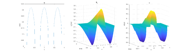
Figure 1: Section 6.1: Plot of $u_{c}$ and the solutions $w$ and $u$ for $\gamma=5$.

$\gamma$	% of $\{u(x)=0\}$ in $\Omega$
$0$	$0$%
$1$	$18.5$%
$5$	$43$%
$10$	$68$%

Table 1: Section 6.1: Percentage of the domain where $u$ vanishes for different values of $\gamma$.

$k$	$\|u_{k}-u_{\lx@mung@bibliography@pre}\thebibliography\lx@bibitem{\|}_{U}$	$\|w_{k}-w_{\lx@mung@bibliography@pre}\thebibliography\lx@bibitem{\|}_{W}$	$|\Phi_{0}(u_{k},w_{k})-\Phi_{0}(u_{\lx@mung@bibliography@pre}\thebibliography\lx@bibitem{,}w_{\lx@bibitem{)}}|$	$\Phi(u_{k},w_{k})$
$10$	$5.5871\text{\cdot}{10}^{-3}$	$1.6573\text{\cdot}{10}^{-2}$	$0.15402$	$1.9887$
$20$	$4.1156\text{\cdot}{10}^{-3}$	$1.2061\text{\cdot}{10}^{-2}$	$0.11178$	$1.9465$
$30$	$3.657\text{\cdot}{10}^{-3}$	$1.0559\text{\cdot}{10}^{-2}$	$0.08259$	$1.9173$
$40$	$2.5632\text{\cdot}{10}^{-3}$	$7.198\text{\cdot}{10}^{-3}$	$0.05709$	$1.8918$
$50$	$5.126\text{\cdot}{10}^{-06}$	$9.6418\text{\cdot}{10}^{-06}$	$0.0233$	$1.858$
$55$	$1.3119\text{\cdot}{10}^{-07}$	$1.9858\text{\cdot}{10}^{-08}$	$0.00835$	$1.8431$
$59$	-	-	-	$1.8347$

Table 2: Section 6.1: Errors for different numbers of iterations for $\gamma=1$.

$N$	$\parallel u{}_h-u{}_{\text{Reference}}$