Atomic clock interferometry using optical tweezers

Abstract

Clock interferometry refers to the coherent splitting of a clock into two different paths and recombining in a way that reveals the proper time difference between them. In contrast to comparing two separate clocks, this type of measurement can test quantum gravity theories. Atomic clocks are currently the most accurate time keeping devices. Here we propose using optical tweezers to implement clock interferometry. Our proposed clock interferometer employs an alkaline-earth-like atom held in an optical trap at the magic wavelength. Through a combination of adiabatic, tweezer-based, splitting and recombining schemes and a modified Ramsey sequence on the clock states, we achieve a linear sensitivity to the gravitational time dilation. Moreover, the measurement of the time dilation is insensitive to relative fluctuations in the intensity of the tweezer beams. We analyze the tweezer clock interferometer and show that it is feasible with current technological capabilities. The proposed interferometer could test the effect of gravitational redshift on quantum coherence, and implement the quantum twin paradox.

I Introduction

Atom Interferometers (AIFs) are techniques for coherently manipulating spatial superpositions of atomic wavefunctions and measuring their phase difference. AIFs come in many forms, yet they all share the same basic steps and structure [1]. The AIF consists of input and output ports, typically two of each type. The ports may be characterized by the outcome of different observables, such as position [2], momentum [3], and angular momentum [4]. A single atomic wavepacket populating one of the input ports is coherently split into two spatially separated wavepackets, so that each wavepacket is traveling on a different path. Each path may be under the influence of a different potential, so that each wavepacket acquires a different phase. After acquiring the phase, the wavepackets are coherently recombined. This process maps the phase difference between the wavepackets to population probabilities at the output ports. The populations are, in turn, measured to infer the phase difference.

The most common type of AIFs is free space light-pulse interferometry, such as the Kasevich-Chu Interferometer (KCI) [3]. In such architectures, atoms in free fall are split and recombined in momentum space through the absorption of photons, thus creating two possible spatial trajectories. An alternative approach is to confine the wave packets in a potential well during all or part of their trajectories. These types of AIFs, also known as guided AIFs, offer several potential advantages over traditional light-pulse AIFs, including arbitrary atom trajectories, precise positioning, long probing times, and compact experimental setups. In recent years, several architectures for guided AIFs have been proposed. Among the methods available for manipulating atomic trajectories are optical lattices [5] and optical tweezers [2, 6, 4].

AIFs, particularly KCI, have been successfully employed in numerous precise measurements [7, 8]. The fact that AIFs involve massive particles and can detect extremely small variations in force fields makes it an excellent choice for gravitational measurements. Indeed, AIFs have been used to test the weak equivalence principle [9] and to determine the gravitational constant [10, 11]. One central tenet of general relativity is the modification of proper time due to masses. Proper time, denoted by $\tau$, is the time measured by an ideal clock moving with the reference frame. The theory of General Relativity predicts that clocks tick slower near a large mass, a prediction confirmed in several experiments comparing independent clocks positioned at different distances relative to Earth’s mass [12, 13, 14, 15, 16, 17].

In principle, time dilation can also be probed using AIF. As proper time is inherently tied to the metric in general relativity, observing its influence on the wavefunction’s interference pattern could probe the regime in which both general relativity and quantum mechanics have a measurable effect [18], allowing tests of quantum gravity theories. As an example, some theories propose treating proper time as a quantum operator, with mass as its conjugate [19, 20]. In these theories, the uncertainty in proper time is predicted to affect the visibility of the interference pattern [21]. Other proposals suggest interferometric measurements to test the connection between gravity and decoherence on macroscopic scales [22, 23].

The phase of a matter wave, $\phi$, is connected to it’s proper time through [24]:

$$\phi=\frac{mc^{2}}{\hbar}\tau\,,$$ (1)

where $m$ is the mass, $c$ is the speed of light, and $\hbar$ is the reduced Planck constant. This relation may lead one to conclude that it is possible to use the accumulated phase in AIF as a means to measure the difference of the proper time. This claim was made by Muller et al. as they reinterpreted light-pulse interferometry experiments as a clock ticking in the Compton frequency, and as such, used its measured phase difference for calculating the gravitational red shift [25]. However, it was claimed that the proper time cannot be measured by a particle with a single internal state [26]. The phase difference in a light-pulse AIF in free fall is only due to the different phases of light pulses relative to the atoms accelerated by gravity, $g$ [24]. To ascertain the proper time difference, it is necessary to employ a clock, which requires at least two internal states. Atomic clock interferometry (ACIF) has not yet been performed.

A natural choice for clock interferometry is optical atomic clocks, which are the most accurate man-made timekeeping devices [27]. These clocks are based on measuring the optical transitions between long-lived electronic states. Their operation relies on cold atom technology, namely the ability to precisely control with light the internal and external degrees of freedom of single atoms [28]. The atoms are held in an optical potential for long probing durations. To eliminate systematic shifts due to light shift, a ‘magic’ wavelength is chosen for the optical potential where the two internal states have equal polarizability [27]. In most atomic clocks, the potential is generated by an optical lattice, but recently the use of optical tweezers has also been reported [29].

A step towards ACIF has been taken using the ${}^{1}S_{0}-{}^{3}P_{0}$ optical clock transition of ⁸⁸Sr [30, 31, 32]. In these experiments, however, the splitting was accomplished using a single photon optical transition. Consequently, the atoms in each interferometer arm were in one of the clock states and not in a superposition of them. Therefore, they did not act as a clock in the sense required for measuring the proper time difference between the arms. Guided ACIFs hold a great promise for gravitational measurements, in particular for testing the Universality of the Gravitational Redshift (UGR) – the principle that the gravitational time dilation is independent of the inner workings of the clock [33, 34]. In most light pulse interferometers, the proper time difference between the arms is zero [24, 35, 36]. Previous works were focused mainly on suggesting ACIFs based on light-pulse schemes that overcome this difficulty [34, 33, 37]. Guided interferometers, on the other hand, are inherently well-suited for measuring differences in proper time. [34]. However, despite the strong motivation to test theories of quantum gravity, a concrete scheme for a guided ACIF has yet to be proposed.

In this work, we propose an ACIF scheme that uses optical pulses only to create a balanced superposition of the clock states in each arm, while the splitting process is achieved by using adiabatic tunneling transitions between optical tweezers. The scheme achieves linear sensitivity to gravitational time dilation, providing a significant signal in realistic experimental timescale. Importantly, we show that when the tweezer is at a magic wavelength, the interference signal is insensitive to relative intensity fluctuations between the tweezers. This property makes an interferometric measurement of the gravitational red shift with our proposed scheme feasible with current technological capabilities. The significance of this experiment lies in measuring a general gravity effect with a spatially separated coherent quantum state for the first time.

The structure of the paper is as follows. In section II we briefly discuss tweezer atomic interferometry, previously proposed in Ref. [2] in relation to atoms with a single internal quantum state. In section III we generalize this scheme for tweezer clock interferometry, using unitary evolution calculations for the expected interference pattern. In section IV we analyze the expected signal in a realistic experimental scenario and demonstrate that it can be measured. We conclude and give an outlook in section V.

II Tweezer atomic interferometry

In Ref. [2], we introduced a guided AIF scheme using optical tweezers. As the ACIF scheme we present in section III builds upon this concept, we briefly revisit it here for clarity. In the tweezer AIF, the atom’s motion is controlled throughout the entire interferometric sequence by manipulating the position of the optical tweezers. The sequence starts with the atoms located in one of the tweezers. Coherent splitting and recombining are achieved by an adiabatic change of the traps’ positions. We proposed two configurations for the splitters and combiners, utilizing either a two-tweezer or a three-tweezer setup.

In the two-tweezer scheme, the trap potential is written as

$$V(x,t)=-V_{0}\left[e^{-2\frac{x-d\left(t\right)/2}{\sigma^{2}}}+\Big{(}1-\Delta\left(t\right)\Big{)}e^{-2\frac{x+d\left(t\right)/2}{\sigma^{2}}}\right]\,,$$ (2)

where $\sigma$ is the waist of the Gaussian beam creating each of the tweezers, $V_{0}$ is the potential depth, and $\Delta(t)$ is the depth difference (detuning) between the two traps. Splitting of the wavefunction is achieved by changing the separation between the traps, $d(t)$, and the detuning in the following manner:

$$d(t)=\frac{1}{2}(d_{max}+d_{min})+\frac{1}{2}(d_{max}-d_{min})\cos\left(2\pi t/T\right)\\$$ (3)

$$\Delta(t)=\begin{cases}\Delta_{max}(1-2t/T)&\text{if }t<T/2\\ 0&\text{if }t\geq T/2\end{cases}\ \ ,$$ (4)

where $T$ is the total splitting process time, and $d_{max}$ ($d_{min}$) is the initial (shortest) distance between the trap centers. The initial seperation is large enough such that tunneling is negligible. The initial detuning, $\Delta_{max}$, is chosen to be the largest possible value before eigenstates with different vibrational numbers cross.

To explain how the splitting works, we consider a single atom which is initially placed in the deeper trap. The splitting sequence is slow enough to be adiabatic and consists of two parts. First, the traps are brought closer to a distance $d_{min}$ and simultaneously the detuning is decreased to zero. Then, the traps are moved back to their initial position while the detuning remains zero. The splitting occurs due to the adiabatic following of the atom’s wavefunction – at the beginning of the process, the atom is in the double-trap’s ground state, located at the deeper trap. The adiabatic modification of the potential ensures that the final atomic wavefunction is still the trap potential’s ground state, which is a balanced symmetrical split between the traps. If an atom is initially placed in the shallower trap, which corresponds to the first excited state of the initial Hamiltonian, it will end in the anti-symmetric split state.

After the splitting phase, the wave packet in each of the interferometer arms acquires a phase at a different rate due to evolution under different potentials. At the end of the phase acquisition stage, the combiner, which is the time-reversal of the splitter, is applied. If the interferometer arms finish the process with a relative phase of 0 ($\pi$) radians, the combiner maps the atom position to the deep (shallow) trap. For any other phase, the final atomic wavefunction will be a superposition of populating each trap, thus achieving a phase-to-population mapping in the combiner step of an interferometer.

The three-tweezer scheme can be explained using the same principle of adiabatic following of the atomic wavefunction. The initial potential has three traps: two at distance $d_{max}$ from both sides of a central trap, and with a detuning $\Delta$ (the central trap is deeper). The atom is initially placed at the center trap, in the ground state of the triple-trap potential. The splitting follows a similar two steps process. First, the distance of the external traps from the center trap is decreased to $d_{min}$ while the detuning is lowered to zero. Then, the external traps are distanced to $d_{max}$ while the detuning is changed to $-\Delta$. The atom ends at the ground state of the final potential, which is the symmetric superposition of being in the two external traps.

Similarly to the two-tweezer case, the combiner is the time-reversal of the splitter sequence. Due to the symmetry of the Hamiltonian, the combiner maps only the symmetric part of the final wavefunction back to the central trap, and leaves the anti-symmetric part unchanged. Therefore, the symmetric part of the final wavefunction is mapped to the central trap and the anti-symmetric part is mapped to the external traps. Any phase difference between the arms maps to a superposition of being in the central and external traps. The larger number of degrees of freedom in the three-tweezer splitter and combiner provides the important benefit of error detection, that is, the possibility to detect and discard runs where, due to experimental imperfections, the splitting or recombining processes were not successful.

An important feature of the optical tweezer AIF scheme is that it can be executed with many atoms in a single run [2]. This is attributable to the fact that the splitting and recombining schemes can work successfully with different initial vibrational eigenstates as long as they are still adiabatic. Running an interferometric measurement with $N$ atoms in different vibrational states is equivalent to $N$ runs with one atom each, allowing for an improvement in the signal-to-noise ratio at a given number of repetitions. Preparation of each atom at a different eigenstate can be achieved by loading the tweezer with fermionic atoms in a single spin state [38].

The guided interferometer architecture with optical tweezers offers several advantages over free-fall light-pulse interferometry. One of the biggest limitations of light-pulse interferometry is that since the atoms are in free-fall and the acquired phase scales as $T^{2}$ [39], better sensitivity requires increasingly larger apparatus. The guided interferometer allows for a long interrogation time while remaining compact. Another limitation of light-pulse interferometry is that the atoms are in free-fall. In the proposed tweezer AIF, the atom’s position is entirely determined by the tweezer position, which allows for arbitrary trajectories during phase accumulation. Due to its enhanced sensitivity and arbitrary atom trajectory, the tweezer AIF can measure effects in classical and quantum gravity, e.g measuring the gravitational constant $G$ [40], testing the Newtonian law at small distances [40], measuring the gravitational redshift [34] and searching for evidence of the gravitational-field quantization [41, 42]. Most importantly, in the context of this paper, guided interferometers are sensitive to proper time differences between the arms [34], while existing light-pulse interferometers are inherently insensitive to proper time [36]. Moreover, an optical tweezer AIF working at a magic wavelength with an atomic clock is ideally suited to measure the gravitational time dilation, as we demonstrate in section III.

III Tweezer clock interferometry

According to general relativity, the proper time, $\tau$, is determined by the metric, $g_{\mu\nu}$, according to

$$\tau=\int_{\Gamma}\,d\tau=\frac{1}{c^{2}}\int_{\Gamma}\sqrt{g_{\mu\nu}\,dx^{\mu}dx^{\nu}}\ \ ,$$ (5)

where the integration is performed along a path $\Gamma$. Clocks that follow different paths may experience a difference in their proper time. In particular, if clocks are positioned at different locations under the influence of a gravitational field, they tick at a different rate. This prediction of general relativity was confirmed using two clocks at different heights [12]. On the other hand, proper time is connected to matter-wave phase through Eq.(1). This serves as a motivation for using a matter-wave interferometer as a probe in situations where both general relativity and quantum mechanics are relevant.

Optical tweezer AIFs, like those discussed in section II, can be used to measure phases arising from proper time differences if the atom has at least two internal states. This is due to the fact that an atom with a single internal degree of freedom cannot produce a periodic signal necessary for measuring proper time [26, 43]. Interferometers employing only a single internal state can only measure effects stemming from a difference of the gravitational potential at different location, analogous to a gravitational Aharonov-Bohm effect [44]. Such observations were made using atomic and neutron interferometry [45]. Atomic clock interferometry was previously proposed as a method to measure proper time differences [33, 37, 34, 43]. However, these proposals suffer from the same limitation of free falling AIF discussed in section II. In what follows, we present a proposal for a guided ACIF, using optical tweezers at a magic wavelength. Our scheme inherits the advantages of the tweezer AIF, namely long probing duration and high position accuracy. Additionally, the measurement of the proper time difference is insensitive to relative intensity fluctuations, which makes it applicable to current tweezer technology.

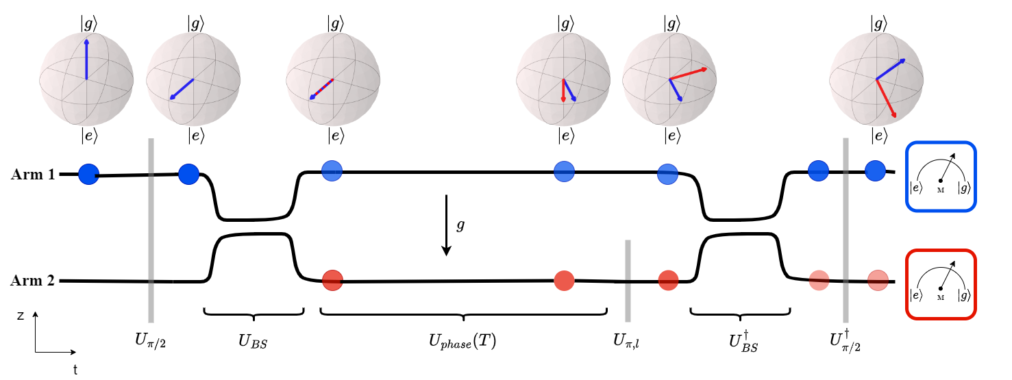
Figure 1: The proposed scheme for interferometry with an atomic clock. The black solid lines represent the tweezers’ centers in 1D (vertical axis) as a function of time (horizontal axis). The upper trap is denoted as 1, and the lower trap as 2. Gray vertical lines represent the optical pulses driving the transitions between the clock states (internal degrees of freedom). The curly brackets indicate the time under the influence of a certain unitary transformation. The opacity and color of the shaded circles indicate the probability to find an atom at a particular spatial mode. $U_{phase}(T)$ marks the evolution for a duration $T$ of the trapped atoms while they are subjected to the earth’s gravitational potential. We depict above the interferometer diagram vectors on the Bloch sphere of the atomic states in the spin-$\frac{1}{2}$-like space spanned by the clock states at each corresponding time. The blue (red) arrows show the state at the upper (lower) arm.

Our guided ACIF scheme is depicted in Fig. 1. It is a modification of the scheme discussed in section II, and can be applied with both the two- and three-tweezer approaches. It employs an atom which can be used as an atomic clock, i.e., with two long-lived internal states, denoted by $\ket{g}$ and $\ket{e}$. We choose the tweezers to operate at the magic wavelength of the clock, where both clock states experience the same trap potential. The atom is initially prepared in the ground state $\ket{g}$. Before the wavepacket splitting stage, a $\pi/2$-pulse of an optical field, which is resonant with the $\ket{g}\leftrightarrow\ket{e}$ transition, is applied. This pulse generates the superposition $\frac{1}{\sqrt{2}}(\ket{g}+\ket{e})$.

Following the $\pi/2$-pulse, the spatial splitting of the clock wavefunction takes place, using either two or three tweezers. Each interferometer arm is moved to a different position in the gravitational field. Therefore, each part of the clock wavefunction experiences a different proper time. Before the recombining phase, a $\pi$-pulse on the $\ket{g}$-$\ket{e}$ transition is applied to only one of the arms. The sequence ends with the spatial recombining of the wavefunction, as described in section II, followed by another $\pi/2$-pulse on the clock degrees of freedom to close the Ramsey sequence. The measured observables are the internal state of the atom and the spatial output port. As we demonstrate below, both quantities are required for a measurement of proper time differences in a coherent superposition of an atom.

To proceed with the calculation, we use a unitary time-evolution operator approach. We label the vectors spanning the relevant Hilbert space by $\ket{k;l}$, where $k=g,e$ and $l=1,2$ denote the internal (clock) and external (paths) degrees of freedom, respectively. The evolution operators employed in the description of the interferometer are defined with respect to the following vectors:

$$\begin{split}\ket{g;1}&\equiv\begin{pmatrix}1,&0,&0,&0\end{pmatrix}\\ \ket{g;2}&\equiv\begin{pmatrix}0,&1,&0,&0\end{pmatrix}\\ \ket{e;1}&\equiv\begin{pmatrix}0,&0,&1,&0\end{pmatrix}\\ \ket{e;2}&\equiv\begin{pmatrix}0,&0,&0,&1\end{pmatrix}\,.\end{split}$$ (6)

After the splitting and before the recombining, we define the energy difference $\Delta E$ (and the corresponding frequency $\omega_{0}$) between the two clock states in path 2 as

$$\Delta E=h\omega_{0}=E_{e;2}-E_{g;2}\,.$$ (7)

We assume that there is a gravitational potential difference between the paths, $\Delta\varphi$, which gives rise to a difference in the proper time. This means that clocks following the different paths tick at a different rate. Therefore, the transition energy between the clock states must depend on the path, since it can be used as a clock. We write this explicitly as

$$E_{e;1}-E_{g;1}=\Delta E+h\epsilon$$ (8)

with $\epsilon=\frac{\omega_{0}}{c^{2}}\Delta\varphi$ being the frequency difference due to the gravitational redshift. Our goal for the ACIF sequence is to allow determination of $\epsilon$. It is important to note that in the way we wrote Eqs.(7-8) we explicitly assumed that the energy difference between the clock states does not depend on the depth of the confining optical potential, which is justified when the trap is operated at the magic wavelength.

To calculate the output of interferometric sequence, we define the unitary operations from which it is composed. $U_{BS}$ is the unitary time-evolution operator corresponding to the spatial wavefunction beam-splitter,

$$U_{BS}=\frac{1}{\sqrt{2}}\begin{pmatrix}1&1&0&0\\ 1&-1&0&0\\ 0&0&1&1\\ 0&0&1&-1\end{pmatrix}\,.$$ (9)

$U_{\pi/2}$ corresponds to a $\pi/2$-pulse over the internal degree of freedom for both interferometer arms,

$$U_{\pi/2}=\frac{1}{\sqrt{2}}\begin{pmatrix}1&0&-1&0\\ 0&1&0&-1\\ 1&0&1&0\\ 0&1&0&1\end{pmatrix}\,.$$ (10)

$U_{\pi,l}$ represents a $\pi$-pulse over the internal degree of freedom in the lower arm only, the upper arm remains unchanged,

$$U_{\pi,l}=\frac{1}{\sqrt{2}}\begin{pmatrix}1&0&0&0\\ 0&0&0&-1\\ 0&0&1&0\\ 0&1&0&0\end{pmatrix}\,.$$ (11)

$U_{\text{phase}}(T)$ corresponds to the phase accumulation stage with a duration $T$,

$$U_{\text{phase}}(T)=\begin{pmatrix}e^{-\frac{i}{\hbar}E_{g;1}T}&0&0&0\\ 0&e^{-\frac{i}{\hbar}E_{g;2}T}&0&0\\ 0&0&e^{-\frac{i}{\hbar}E_{e;1}T}&0\\ 0&0&0&e^{-\frac{i}{\hbar}E_{e;2}T}\end{pmatrix}\,.$$ (12)

The final state after our proposed ACIF sequence can be written as

$$\ket{\psi_{f}}=U_{\pi/2}^{\dagger}U_{BS}^{\dagger}U_{\pi,l}U_{\text{phase}}(T)U_{BS}U_{\pi/2}\ket{g;1}\,.$$ (13)

Following the sequence there are two types of observables one can measure. The first observable is the spatial output port of the atom. The probability of the atoms to exit the interferometer from the upper port is given by

$$\begin{split}&P_{1}(\psi_{f})=P_{g;1}+P_{e;1}=|\langle g;1|\psi_{f}\rangle|^{2}+|\langle e;1|\psi_{f}\rangle|^{2}=\\ &=\frac{1}{2}\left[1-\sin\left(T\left(E_{g;1}-E_{g;2}+\frac{\epsilon}{2}\right)\right)\sin\left(T\left(\omega_{0}+\frac{\epsilon}{2}\right)\right)\right]\,.\end{split}$$ (14)

A crucial requirement for an interferometric measurement is the ability to verify that the atom was indeed in a coherent superposition during the sequence. The result of Eq.(14) allows this, since it exhibits coherent oscillations between the exit ports as a function of $T$. In contrast, if the wave packet collapses randomly to one of the paths and the state becomes completely mixed, the exit port is $P_{1,\text{mixed}}(\psi_{f})=\frac{1}{2}$. This means that measuring oscillations around the probability of $\frac{1}{2}$ as a function of time verifies the coherence of the atomic wavefunction.

The main disadvantage of measuring the spatial output port is the exit probability dependence on the difference between the eigenenergies: $E_{g;1}-E_{g;2}$. This makes this observable sensitive to relative fluctuations between the intensity of the trap beams. There are two ways to cope with this issue. On one hand, one can set stringent requirements on the laser intensity stability throughout the interferometer time which will ensure low noise in this measurement. This approach can be very challenging experimentally. An alternative approach is to acknowledge that the fluctuations exist and result in almost a random phase in the first sine term of Eq.(14). The probability distribution, $P(x)$, of $x=\sin(\phi)$ with $\phi$ being evenly and randomly distributed is $P(x)=(\pi\sqrt{1-x^{2}})^{-1}$. Thus, if the wave packet is coherently split and held, the distribution of $P_{1}$ should follow $P(x)$ over a dataset large enough.

The second available observable is the inner clock state of the atom. The probability of the atoms to be in the clock ground state at the end of the sequence is given by

$$\begin{split}P_{g}(\psi_{f})&=P_{g;1}+P_{g;2}=|\langle g;1|\psi_{f}\rangle|^{2}+|\langle g;2|\psi_{f}\rangle|^{2}\\ &=\frac{1}{2}\left[1-\sin\left(T\left(\omega_{0}+\frac{\epsilon}{2}\right)\right)\sin\left(T\frac{\epsilon}{2}\right)\right]\,.\end{split}$$ (15)

As is readily seen from Eq.(15), in contrast to the case of measuring the spatial output port, the probability to finish in the ground state depends only on $\omega_{0}$ and $\epsilon$, but not on the eigenenergies separately. This means that this observable is insensitive to relative fluctuations in the depths of the tweezers, which would shift the eigenenergies, but do not affect $\omega_{0}$, as long as we operate at the magic wavelength.

The probability to be in the ground state is the same whether the state is coherent or mixed. Therefore, it is essential to measure both the spatial output port and the internal state of the atom. The measurement of the output port will ensure the coherence of the atomic state, while the measurement of the internal state, which is robust in the presence of laser intensity noise, will be used to extract $\epsilon$.

The redshift is extracted from Eq.(15). By scanning the waiting time, $T$, the probability to find the atoms in the ground state oscillates due to interference of the two paths. The oscillation frequency of this interference pattern is the average clock frequency in the two paths $\omega_{0}+\frac{\epsilon}{2}$. Its visibility is given by

$$\mathcal{V}=\sin(T\frac{\epsilon}{2})\,.$$ (16)

The amplitude of the expected oscillating interference is determined by $\epsilon$, which gives us a straightforward way to extract this observable. Importantly, for small redshifts ($T\epsilon\ll 1$), the visibility scales linearly with $\epsilon$: $\mathcal{V}\approx T\epsilon/2$. This should be contrasted with a similar interferometric sequence, only without the $\pi$ pulse in the lower path. In that case, the visibility of the interference pattern scales as $\mathcal{V}\approx 1-(T\epsilon)^{2}/8$. The linear scaling of the visibility in our scheme is crucial to make an experimental observation feasible, as we illustrate below.

IV Feasibility analysis

We now turn to estimate the measurable effect in a realistic experimental scenario. The redshift is

$$\epsilon=\frac{\omega_{0}}{c^{2}}\Delta\varphi=\frac{\omega_{0}}{c^{2}}mg\Delta h\,\,,$$ (17)

with $\Delta h$ being the height difference between the two interferometer arms. Since the effect is linear in atomic mass, it is beneficial to use a relatively massive species. Therefore, we take the atom to be ¹⁷¹Yb, with the clock transition being ${}^{1}S_{0}-{}^{3}P_{0}$. The energy difference between the clock states corresponds to optical emission with a wavelength of approximately $\lambda=578nm$. The magic wavelength of the tweezer trap for this atom is around $\lambda_{\text{magic}}=759nm$ [46].

Similar to Ref. [2], we assume a separation between the two tweezer arms of 10 mm, aligned in the same direction as Earth’s gravitational acceleration, $g$. Taking a phase accumulation duration of $T=10s$, we obtain a visibility of $\mathcal{V}\approx 0.02$. The oscillating signal appears on top of a background signal of 0.5. Assuming a $1/\sqrt{N}$ scaling of the noise with the number of measurements, it follows that more than $N>625$ measurements are needed to achieve a signal-to-noise ratio better than one. Factoring in an overhead of 5 seconds for each run, the total duration per run extends to 15 seconds. In the worst case scenario where only a single atom is utilized per run, it would take approximately 2.5 hours of data collection for the gravitational time dilation effect to become discernible. Given that the interferometer allows for multiple atoms per run, the effective runtime to achieve a specified signal-to-noise ratio is expected to be significantly reduced.

Operating two optical Ramsey-like pulses coherently over a span of 10 seconds implies a requirement for a narrow linewidth of the clock laser. This requirement is similar to what is needed in light-pulse interferometers using the optical transition in ⁸⁸Sr [47]. Indeed, state-of-the-art laser systems built for atomic clocks can reach a linewidth below 10 mHz [48], achieving coherence times that exceed 10 seconds [29]. For the estimation of the redshift measurement previously described, such a laser is sufficient.

An alternative approach is to use a commercially available laser with a larger linewidth, but prolong its coherence time using the Yb atoms. This can be done, for example, through phase-locking the laser to the atomic clock transition with quantum non-demolition (QND) measurements [49]. Such methods were able to achieve clock coherence time on the order of 1-5 seconds. Interferometry time of 1 second will result in a visibility $\mathcal{V}\approx 0.002$. Assuming the same overhead time, this will require integrating data over approximately 11 days when working with a single atom, or about a day, if 10 atoms are used in each run. Either way, we conclude that the observation of gravitational redshift with ACIF is within the reach of current technological capabilities.

V Discussion

We introduce a guided atomic clock interferometer approach, an extension of our previous tweezer interferometer method [2], tailored for atoms with two internal states. This technique employs optical laser pulses to create a superposition of the internal states and utilizes precise manipulation of the tweezers’ position and intensity for the spatial adiabatic splitting and recombining of the wave packet. After completion of the interferometric scheme, we record the population within each clock state and exit port. The coherent oscillations observed between the two exit ports confirm the wave packet’s spatial coherence throughout the experiment. Oscillations between the internal states reveal time dilation across the paths. In particular, the visibility of these oscillations is instrumental in determining the gravitational redshift between the interferometer arms. Clock interferometry, which has not been performed to date, is achievable using our proposed scheme with the current state of technology.

Quantum theory has been tested successfully in many experiments, including with atomic interferometry. Similarly, predictions of General Relativity have also been verified, including measurements of the gravitational redshift using two separate clocks [12, 13, 14, 15, 16, 17]. However, theories of quantum gravity in regimes in which both quantum mechanics and general relativity are relevant remain untested. The proposed ACIF could probe this unexplored regime for the first time [18].

One theory on the intersection of quantum mechanics and general relativity suggests that gravitational redshift contributes to the decoherence observed in the classical limit [22]. In the context of a clock interferometer, the gravitational field causes entanglement between the atom’s internal state and its spatial wavefunction. In a larger scale scenario, a body composed of many such internal degrees of freedom can be viewed as multiple clocks operating at varying rates, influenced by the gravitational field. This variance in ticking rates leads to dephasing among the clocks and consequently reduction in coherence for the spatial wavefunction. This offers a potential explanation for decoherence in the classical limit that does not rely on interaction with environment. Using an ACIF to test the case of a single clock is a first step towards testing the effect of gravity on the coherence of macroscopic objects.

An ACIF experiment may also have implications for theories of quantum time. In general relativity, time is dynamic and dependent on the metric, functioning as a dimension. Conversely, quantum theory treats time as a global parameter. To resolve this discrepancy between general relativity and quantum theory, there have been suggestions for a dynamic quantum time operator [50, 51]. Some of these suggestions advocate for considering proper time as the quantum operator with mass being its conjugate. This allows for a quantum operator representation of mass as well [20, 19]. If proper time is represented by a quantum operator, its uncertainty could influence the expected visibility of an ACIF experiment. Therefore, measuring deviations from the expected result could help constrain theories of quantum proper time [21].