Parsimonious Generative Machine Learning for Non-Gaussian Tail Modeling and Risk-Neutral Distribution Extraction

Abstract

In financial modeling problems, non-Gaussian tails exist widely in many circumstances. Among them, the accurate estimation of risk-neutral distribution (RND) from option prices is of great importance for researchers and practitioners. A precise RND can provide valuable information regarding the market’s expectations, and can further help empirical asset pricing studies. This paper presents a parsimonious parametric approach to extract RNDs of underlying asset returns by using a generative machine learning model. The model incorporates the asymmetric heavy tails property of returns with a clever design. To calibrate the model, we design a Monte Carlo algorithm that has good capability with the assistance of modern machine learning computing tools. Numerically, the model fits Heston option prices well and captures the main shapes of implied volatility curves. Empirically, using S&P 500 index option prices, we demonstrate that the model outperforms some popular parametric density methods under mean absolute error. Furthermore, the skewness and kurtosis of RNDs extracted by our model are consistent with intuitive expectations. More generally, the proposed methodology is widely applicable in data fitting and probabilistic forecasting.

1 Introduction

It has been extensively documented that non-Gaussian tails exist widely in financial markets (Rachev, 2003; Jondeau et al., 2007). Moreover, generally, the tails are asymmetric on the left and the right sides (Cont, 2001; McNeil et al., 2015). To avoid the concern of using Gaussian assumption, many advanced distributions were developed, such as the normal inverse Gaussian distribution (Barndorff-Nielsen, 1997), the hyperbolic distribution (Barndorff-Nielsen, 1977), the variance gamma distribution (Madan and Seneta, 1990), the generalized skewed $t$ distribution (Theodossiou, 1998), and so on. Most of them are defined via a relatively complicated density function, which restricts the flexible usage in numerical applications. While the advantage is the analytical tractability, the disadvantages are still significant, such as the inconvenient sampling, the difficult computation of the expectation of a function of the random variable, the further optimization of it, and the optimization of the conditional densities.

Derivatives are very versatile instruments and options are a big family. Option pricing and related topics have long been an active and crucial research area. In mathematical finance, researchers usually make a set of assumptions about what stochastic processes the return and the volatility follow. It ends with a parametric model that takes some market signals as the inputs, then outputs the corresponding option price. The seminal work Black-Scholes-Merton model in Black and Scholes (1973) initiated modern derivatives pricing theories by giving theoretical prices for vanilla European options, by taking the Gaussian assumption. Since then, many studies have been carried out on finding better option pricing models that allow more complex distributions for asset returns, such as the Heston model in Heston (1993) which is widely used now.

Besides, the direct extraction of the risk-neutral distribution (RND), which is the distribution of the future underlying asset price/return in the risk-neutral world, is of great importance for both researchers and market practitioners. Theoretically, option prices reflect information about the financial market, represent the market’s expectations on the future, and provide a path for investments and risk management. The temporal behavior of the second moment of the market index’s RND is a barometer for monitoring the systemic risk or is the proxy of a risk factor. More specifically, risk-neutral higher moments or other distributional characteristics such as skewness, kurtosis, and quantiles derived from the estimated RND can have informational content or predictive power with economic significance in empirical asset pricing studies (Bali and Murray, 2013; Völkert, 2015; Stilger et al., 2017; Wong and Heaney, 2017; Chordia et al., 2021; Fuertes et al., 2022). Furthermore, when RND is extracted from the market quotes of several options, we can use it to price other options for trading and hedging purposes. Given an accurate RND, any path-independent option can be priced precisely.

Many researchers proposed various methods for recovering RND from market quotes of options. Christoffersen et al. (2013) provided a comprehensive review of the literature and summarized the comparisons among these articles. Figlewski (2018) reviewed the major ideas in this field. Generally, the methods extracting RND include parametric methods, semi-parametric methods, and non-parametric ones, based on how they express the distribution.

Parametric methods are the most popular ones, for there are lots of existing parametric distributions available for use. In Fabozzi et al. (2009), researchers summarized parametric distributions including Weibull, generalized beta, and generalized gamma for recovering RND. Among the parametric methods, mixture models are the most widely used ones for their flexibility and parsimony, e.g., the double log-normal distribution in Bliss and Panigirtzoglou (2002). Semi-parametric methods include expansion ones such as Edgeworth expansion in Jarrow and Rudd (1982). Also, Madan and Milne (1994) used a Hermite polynomial approximation. By combining the Fourier cosine series method and Dirac Delta function with the Carr-Madan spanning formula, Cui and Yu (2021) and Cui and Xu (2022) presented their model-free methods to extract the RND. Albert et al. (2023) extrapolated implied volatilities by parametrizing only the tail with Generalized Extreme Value (GEV) distribution.

It is commonly known that RND can be derived from the second partial derivative of the call value with respect to the strike price. Therefore, a way to calculate an RND non-parametrically is smoothing and filling in the option price curve or implied volatility curve as a function of the strike price first, and then calculating the second partial derivative. The non-parametric methods also contain the use of neural networks for option pricing. Ackerer et al. (2020) presented a neural network approach to fit the implied volatility surface. In contrast, many others concentrate on modeling the option price directly using a neural network with option parameters as inputs, as concluded in Ruf and Wang (2020). Besides, the spline method is also a non-parametric way, such as in Figlewski (2008); Reinke (2020). Figlewski (2008) proposed using a fourth-order spline to interpolate the observed implied volatilities. Orosi (2015) parametrized the call value as a function of the strike price, and the RND is derived using the second partial derivative again non-parametrically.

Parametric models assume functional forms that provide economic interpretation for their parameters. Semi-parametric methods are less popular because they are more complicated mathematically. Non-parametric methods always need to specify certain tuning parameters, which are subjective and unstable, and they cannot produce explicit distributions, which is not friendly for further use. The spline methods cannot capture the tails well because option prices span only over a discrete amount of strike prices, and sometimes deep OTM options would be excluded from the RND estimation process, as shown in Reinke (2020). To mitigate this problem, parametric methods may work well by assuming a reasonable heavy-tail distribution. Parametric methods are also easy to calibrate and easy to compute risk-neutral moments or distributional characteristics. Given their merits, we mainly focus on parametric methods in this paper.

Inspired by these and motivated by the recent successes of machine learning, we propose to tackle the problem with a prevalent and promising approach called the generative machine learning. More specifically, it is a parsimonious parametric model that can describe a rich class of distributions by transforming a base random variable like Gaussian. We aim to recover the risk-neutral distribution of the underlying asset return in the real financial market with the consideration of asymmetric non-Gaussian tails. The probability of extreme loss is higher than the probability estimated with the Gaussian assumption, which is the main reason for the volatility smiles after the market crash of 1987. Therefore, the key to the problem is to allow asymmetrically non-Gaussian tail behavior in the model. We successfully achieve this and show the merits of the proposed method by extensive numerical results in this paper.

We highlight the main contributions of this paper below:

1. The paper introduces the use of a parsimonious generative machine learning model to tackle the problem of non-Gaussian tail modeling and risk-neutral distribution extraction.

2. The proposed method has several advantages compared to traditional density-based methods, such as the asymmetrical non-Gaussian tails, the easy calibration, and the convenient computation of risk-neural distributional characteristics/moments.

3. The method performs well in self-calibration, in calibrating to Heston option prices, and in calibrating to market option prices. The skewness and kurtosis of the extracted risk-neutral distributions of S&P 500 returns are consistent with intuitive expectations.

The rest of the paper is organized as follows. In Section 2, we introduce the necessary background and our motivation from the area of generative machine learning. Section 4 depicts the whole picture of our methodology, with an algorithm described. The experimental studies appear in Section 5. At last, we conclude our paper in Section 6.

2 Background and Motivation

There were many distributions proposed in financial literature that depart from Gaussian. Some of them aim at modeling the real-world or physical distributions, such as the ones mentioned in the beginning of Section 1, while some others are used in risk-neutral worlds. This paper focuses on the risk-neutral distribution, but the methodology here is general and is applicable in both of the two worlds.

2.1 Some Existing Methods for RND Extraction

It is first necessary to specify the form of the risk-neutral distribution. Then the estimation/calibration of the distribution must be done given the market option prices. Many forms of distributions have been proposed in the previous literature, and we choose three popular ones to show below.

Double Log-Normal Distribution (DLN). Bahra (1996), Söderlind and Svensson (1997), and Melick and Thomas (1997) were the first three describing the risk-neutral distribution with a mixture of distributions. A mixture of densities is a convenient way to extend the flexibility, to better describe the data statistically. For the options, the mixture of log-normal densities is a well-known distribution for the reason that it contains the single log-normal and can be viewed as an extension of the Black-Scholes-Merton model. The log-normal density with mean $\mu$ and volatility $\sigma$ is defined by:

$$l\left(s_{T};\mu,\sigma\right)=\frac{1}{s_{T}\sqrt{2\pi\sigma^{2}}}\exp\left(-\frac{1}{2}\left(\frac{\log\left(s_{T}\right)-\mu}{\sigma}\right)^{2}\right).$$

The mixture of two such densities yields:

$$q\left(s_{T};\theta\right)=\sum_{i=1}^{2}\alpha_{i}l\left(s_{T};\mu_{i},\sigma_{i}\right).$$

Here $q\left(s_{T};\theta\right)$, where $\theta=\left\{\mu_{i},\sigma_{i},\alpha_{i},i=1,2\right\}$, is used as the risk-neutral density function of the underlying asset price $S_{T}$ at time $T$.

Generalized Beta Density (GB). Bookstaber and McDonald (1987) proposed the generalized beta distribution to model the risk-neutral distribution. Denote that $a>0$ is the power parameter, $b>0$ is the scale parameter, $v>0$ is the first beta parameter, and $w>0$ is the second beta parameter. Let $B$ be a beta random variable with parameters $v$ and $w$, then $X=b(B/(1-B))^{1/a}$ is a generalized beta with parameters $(a,b,v,w)$. For the complete density function which is much complicated, please refer to Bookstaber and McDonald (1987); Jondeau et al. (2007).

Edgeworth Exapnsion (EW). As mentioned in Jondeau et al. (2007), Jarrow and Rudd (1982) captured deviations from log-normality by an Edgeworth expansion of the risk-neutral distribution around the log-normal distribution. Letting $Q$ be the cdf of the price random variable $S_{T}$, Jarrow and Rudd (1982) showed that an Edgeworth expansion in densities for the true probability distribution $Q$ around the log-normal cdf $L$ can be written up to order 4 with cumulants. With some assumptions, the price of a European call option with strike price $K$ can be approximated. The implied volatility, skewness, and kurtosis can be estimated with nonlinear least squares using this expression.

Other nonparametric or semi-parametric methods. There were several nonparametric or semi-parametric methods proposed in the literature. Monteiro and Santos (2022) proposed a nonparametric kernel function approach with efforts of dealing with convexity, monotonicity, and no-arbitrage. Abadir and Rockinger (2003) and Bu and Hadri (2007) proposed the semi-parametric density functionals based on confluent hypergeometric functions (DFCH). For more methods, please also refer to the introduction section. For comparisons among various methods, please refer to Santos and Guerra (2015); Lu (2019); Ammann and Feser (2019). As we have argued in the introduction section, parametric methods for modeling RND directly have merits such as the tail properties inherently incorporated, the ease of calibration/recovering, and the ease of computing risk-neutral distributional characteristics/moments, so we mainly consider parametric methods in this paper.

2.2 Generative Machine Learning

Recent successful generative machine learning (GML) models embrace a completely different paradigm for modeling a distribution. The density function or distributional function is not the objective anymore. Instead, a new methodology of latent variable transformation is adopted. To be specific, a latent random vector or variable $Z$ having a commonly-known distribution (e.g., Gaussian) is assumed, and the target variable(s) $Y$ of interest (e.g., the observations in a dataset) is assumed to be generated by

$$Y=F_{\Theta}(Z),$$ (1)

where $F_{\Theta}$ is usually a deep neural network that needs to be learned to make $Y$ distributed closely to the observed data. In different generative models, there are different choices for $F_{\Theta}$ and different learning strategies for $\Theta$. The most common ones include Variational Autoencoder (VAE) (Kingma and Welling, 2014), Generative Adversarial Net (GAN) (Goodfellow et al., 2014), Normalizing Flow (NF) (Papamakarios et al., 2021), and their plentiful variants.

The generative models mentioned above have made great achievements in modeling and generating image data, time series, and so on. They all use a deep neural network as $F_{\Theta}$ since the data is usually high-dimensional and exhibits a low-dimensional manifold structure. Such a premise may not be the case in this paper. In a financial market which is a highly risk-sensitive world, modeling a distribution needs an elaborate description of how it is apart from Gaussian, such as on the tail behavior or the asymmetry. Wu and Yan (2019) proposed a non-Gaussian distribution in the form of a quantile function for Value-at-Risk (VaR) prediction in financial markets. It is equivalent to choosing a standard Gaussian-distributed $Z$ in Equation (1) and carefully designing an $F_{\Theta}$ to make $Y$ have asymmetric left and right non-Gaussian tails. We adopt such an idea in this paper for the choice of risk-neutral distribution, since it has some unique merits as we will see in the rest of the paper.

An important general merit of such generative models over traditional density-based distribution modeling approaches is the convenience for sampling. Despite the lack of a closed-form density function, it is very easy to sample from Equation (1) by generating a realization of $Z$ and feeding it into $F_{\Theta}$. This is extremely useful in the financial world, where we may need Monte Carlo simulation throughout, especially in derivatives markets. The density-based sampling undoubtedly brings difficulties. Some arguments state that the density-based approach is easier to do the estimation with the maximum likelihood. By choosing $F_{\Theta}$ as a bijection, the density of $F_{\Theta}(Z)$ can be easily computed numerically and the maximum likelihood estimation can be conducted too. Moreover, when $Z$ is univariate and $F_{\Theta}$ is strictly increasing, the estimation can be done via quantile regression, which is effective and stable, as shown in Wu and Yan (2019).

Besides, the density-based approach suffers in the optimization, because many densities with asymmetric non-Gaussian tails are complicated in mathematical forms. When estimating conditional distributions, or when computing and optimizing the expectation of a function of the random variable, the complicated densities will show their shortcomings. In this paper, we are confident about learning a succinct and effective latent-based generative model with merits for risk-neural distribution extraction. Meanwhile, risk-neutral moments or distributional characteristics such as volatility, skewness, and kurtosis can be easily computed through simulating with Equation (1).

3 Parsimonious Generative Machine Learning

It is commonly known that asset returns in both physical worlds and risk-neutral worlds exhibit asymmetry and non-Gaussian tails. The impact of asymmetry and non-Gaussian tails of RND on the shape of the implied volatility curve is intuitive. Given the fact that real implied volatility curves may exhibit smile, skew, or slope, it is natural to design a distribution family with asymmetry and non-Gaussian tails for RND. This is also useful and meaningful for modeling distributions in physical worlds.

3.1 An Existing Parsimonious GML Model

First proposed by Wu and Yan (2019) and further modified by Yan et al. (2019), researchers proposed a novel parametric quantile function to represent a univariate distribution for asset returns in the physical world. It is a monotonically increasing nonlinear transformation of the standard Gaussian quantile function $\Phi^{-1}(\alpha),~{}\alpha\in(0,1)$:

$$Q(\alpha\mid\mu,\sigma,u,v)=\mu+\sigma\Phi^{-1}(\alpha)\left(\frac{u^{\Phi^{-1}(\alpha)}}{A}+\frac{v^{-\Phi^{-1}(\alpha)}}{A}+1\right),$$ (2)

where $\mu$ and $\sigma$ are location and scale parameters, and $A$ ($=4$) is a hyperparameter to normalize the distribution. The resulting quantile function $Q(\alpha\mid\mu,\sigma,u,v)$ has (heavier) non-Gaussian right and left tails controlled by the parameters $u\geq 1$ and $v\geq 1$. We can observe a reversed S shape in the Q-Q plot of $Q(\alpha\mid\mu,\sigma,u,v)$ against $\Phi^{-1}(\alpha)$. Specifically, the parameter $u$ controls the up tail of the inverted S shape, representing the right tail of the corresponding distribution, while the parameter $v$ controls the down tail, representing the left tail of the corresponding distribution. The larger they are, the heavier the tails are. Setting $u$ or $v$ to 1 results in an exactly Gaussian tail.

We demonstrate the impact of these two parameters on the density function of $Q(\alpha\mid\mu,\sigma,u,v)$ in Figure 1, with the solid line representing the normal distribution when $u=v=1.0$ for reference. We obtain a right heavier tail than Gaussian by setting $u=5.0$ and $v=1.0$, and a left heavier tail than Gaussian by setting $u=1.0$ and $v=4.0$. Due to the monotonic property of the transformation on $\Phi^{-1}(\alpha)$, the inverse of $Q(\alpha\mid\mu,\sigma,u,v)$ is uniquely determined and is a distributional function. Also because of the monotonic property, this methodology is equivalent to applying the same transformation:

$$Y=\mu+\sigma Z\left(\frac{u^{Z}}{A}+\frac{v^{-Z}}{A}+1\right),$$ (3)

to the standard Gaussian variable $Z\sim\mathcal{N}(0,1)$. The random variable $Y$ has exactly the quantile function $Q(\alpha\mid\mu,\sigma,u,v)$. Because the transformation in Equation (3) is strictly increasing, the density of $Y$ can be easily computed numerically, and hence the parameter estimation (unconditional or conditional) given observed data can be done by either maximum likelihood or quantile regression (using Equation (2)).

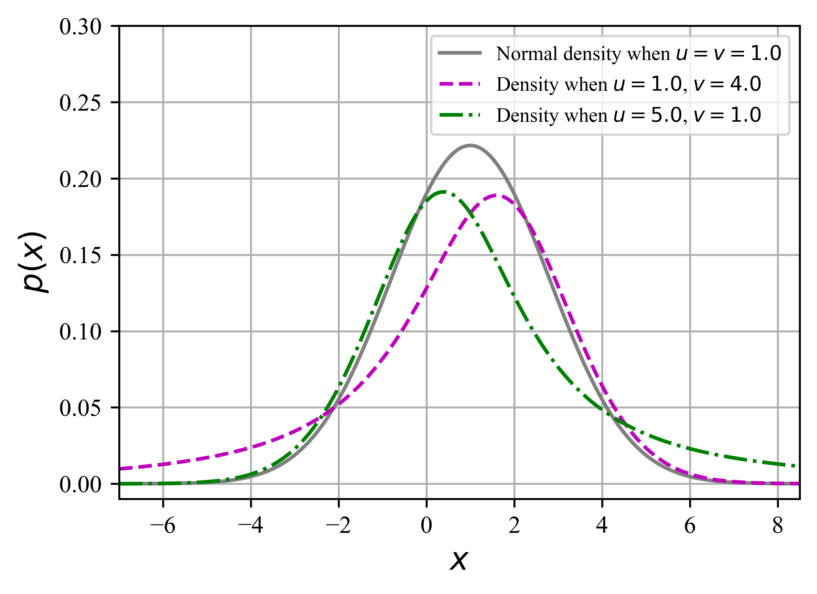
Figure 1: Density functions of the distributions given by Equation (2) or (3), when changing the tail controlling parameters $u$ and $v$. The solid line is the Gaussian density function when $u=v=1.0$ for reference. The dash-dotted line is plotted by setting $u=5.0$ and keeping $v=1.0$, and the dash line is plotted by setting $v=4.0$ and keeping $u=1.0$. We can see that the tail associated with $u=1.0$ or $v=1.0$ is nearly the same as Gaussian tail. Larger $u$ or $v$ produces a heavier tail than Gaussian.

3.2 Generalization and Results on Non-Gaussian Tails

In this part, we generalize the above model to allow more flexible asymmetric non-Gaussian tails. The above model includes a fact that a strictly increasing transformation on the random variable is equivalent to the quantile function transformation. Our aim here is to define such transformations that can conveniently incorporate the tail properties and asymmetry characteristics with intuitive parameters. To begin with, we illustrate our definition of relative tail heaviness.

Given a cumulative distribution function $F$, we denote its survive function $1-F(x)$ as $\bar{F}(x)$. We always assume $F$ is continuous and strictly increasing in an infinite interval, thus the quantile function $F^{-1}$ exists and is also continuous and strictly increasing. We also denote $f(x)\sim g(x)$ if $\lim_{x\to\infty}f(x)/g(x)$ is a positive constant and $\lim_{x\to\infty}f(x)=\lim_{x\to\infty}g(x)=0\text{ or }\infty$. The symbol $\infty$ means either positive infinite or negative infinite.

Definition 1.

We say two distributions have the same left/right tail heaviness if their cumulative functions satisfy $F_{1}(x)\sim F_{2}(x)$ as $x\to-\infty$ or $\bar{F_{1}}(x)\sim\bar{F_{2}}(x)$ as $x\to+\infty$. On the other hand, we say one distribution $F_{2}$ has a heavier right tail than another distribution $F_{1}$ if they satisfy:

$$\lim_{x\to+\infty}\frac{\bar{F_{2}}(x)}{\bar{F_{1}}(\frac{x-\mu}{\sigma})}=+\infty,\quad\forall\mu\in\mathbb{R}\text{ and }\sigma>0.$$ (4)

And the left-side tail heaviness comparison is defined in a similar way.

Definition 2.

We also say two distributions have the same left/right tail heaviness if there exists $\mu\in\mathbb{R}$ and $\sigma>0$ such that $F_{1}((x-\mu)/\sigma)\sim F_{2}(x)$ as $x\to-\infty$ or $\bar{F_{1}}((x-\mu)/\sigma)\sim\bar{F_{2}}(x)$ as $x\to+\infty$.

The first definition says that tail heaviness means $\bar{F_{2}}$ goes to 0 more slowly than any location-scale transformation of $\bar{F_{1}}$, which is consistent with the location-scale transformation of the corresponding random variable. The second definition is an extension, whose intuitive examples are that all normal distributions share the same tail heaviness, all exponential distributions share the same tail heaviness, and all distributions with a fixed tail index share the same tail heaviness. It is easy to show that this definition of equivalent tail heaviness is an equivalence relation in algebraic. The proof is straightforward and is omitted.

Proposition 1.

The equivalent tail heaviness in Definition 2 is an equivalence relation on the set of all distributions that are continuous and have non-zero density on the left (or right) tail side.

3.2.1 A General Form of Transformation

The way we picture a new distribution in this work is very different from traditional methods. Briefly, we construct a totally new distribution with arbitrary tail heaviness by designating its quantile function through a transformation of a known base quantile function (equivalently, through random variable transformation). We start from the general idea and introduce our method as generally as possible, with some specific examples followed.

Firstly, we propose a general form of transformation as follows.

Definition 3.

We define a function $y=f(x),~{}x\in\mathbb{R}$ described as follows to curve the straight line $y=\mu+\sigma x$ in the coordinate plane of $(x,y)$:

$$f(x)=\mu+\sigma x\left(g_{1}(x)+g_{2}(x)+1\right),$$ (5)

where $\sigma>0$, and $g_{1}(x),g_{2}(x)$ satisfy

1. both are differentiable at $x\neq 0$ and continuous at $x\in\mathbb{R}$,

2. $g_{1}(x)$ is monotonically non-decreasing and $g_{2}(x)$ is monotonically non-increasing,

3. $\lim_{x\to-\infty}g_{1}(x)=0$ and $\lim_{x\to+\infty}g_{2}(x)=0$.

In this definition, it is obvious that $g_{i}(x)\geq 0,~{}\forall x\in\mathbb{R},~{}i=1,2$. So $f(x)$ approaches $-\infty$/$+\infty$ as $x$ tends to $-\infty$/$+\infty$. Moreover, $f(x)$ is differentiable over $(-\infty,+\infty)$. At $x=0$, $f^{\prime}(0)=\lim_{x\to 0}\sigma(g_{1}(x)+g_{2}(x)+1)=\sigma(g_{1}(0)+g_{2}(0)+1)$. Next we prove the monotonic property of $f(x)$. If $f(x)$ is strictly increasing, then $f^{-1}(x)$ uniquely exists on $(-\infty,+\infty)$ and is differentiable.

Proposition 2.

If $g_{1}(x)$ and $g_{2}(x)$ satisfy the three conditions in Definition 3 and an additional condition: $g_{i}(x)+xg_{i}^{\prime}(x)>-1/2,~{}\forall x\neq 0,~{}i=1,2$, then $f(x)$ in Equation (5) is strictly increasing.

Proof.

It can be proved from $f^{\prime}(x)=\sigma\left(g_{1}(x)+g_{2}(x)+1\right)+\sigma x\left(g_{1}^{\prime}(x)+g_{2}^{\prime}(x)\right)>0$ at $x\neq 0$ and $f^{\prime}(0)=\sigma(g_{1}(0)+g_{2}(0)+1)>0$. ∎

This additional condition can be easily satisfied, and thus flexible choices for $g_{i}(x)$ are available. For example, for $g_{1}(x)$, the inequality $g_{1}(x)+xg_{1}^{\prime}(x)\geq 0>-1/2$ always holds when $x>0$. As to $x<0$, one can choose a $g_{1}(x)$ that has small $g_{1}^{\prime}(x)$ around 0 and satisfies $\lim_{x\to-\infty}xg_{1}^{\prime}(x)=0$. A simple choice for $g_{1}(x)$ is $g_{1}(x)=\mathbb{I}_{\{x\geq 0\}}x^{u},~{}u>1$. $g_{2}(x)$ can be defined symmetrically, with a different parameter $u$. Intuitively, $y=f(x)$ curves the straight line $y=\mu+\sigma x$ and forms an inverted S shape with fattened tails, while $g_{1}(x)$ and $g_{2}(x)$ acting on the upper and lower side respectively. Next, we apply this transformation on a base random variable and equivalently on its quantile function.

Proposition 3.

Suppose $F(x)$ is the cumulative distribution function of a random variable $X$ and its inverse $F^{-1}(\alpha)$, $\alpha\in(0,1)$ is the quantile function. If $f(x)$ satisfies the four conditions in Proposition 2, then the new function $f(F^{-1}(\alpha))$ is the quantile function of the new random variable $Y=f(X)$, i.e., its inverse $F(f^{-1}(x))$ exists and is the cumulative distribution function of $Y=f(X)$.

Proof.

It is straightforward according to the three properties of $f(x)$: strictly increasing, differentiable, and approaching $-\infty$/$+\infty$ over $(-\infty,+\infty)$. ∎

This leads to an easy simulation property of our method, which is a great advantage compared to the traditional heavy tail modeling approach. To simulate from the distribution of $Y$, we only need to sample from a simpler base distribution of $X$ and then apply the transformation $f$. This convenience is particularly important and useful in financial applications such as derivatives pricing and risk management. Besides, again, the parameter estimation (unconditional or conditional) given observed data can be done by either maximum likelihood or quantile regression, because both of them can be easily computed given a simple base distribution of $X$.

3.2.2 Some Examples

Here, the distribution $F(x)$ is referred as the baseline distribution. Typically we are focusing on the tail behavior of the new distribution, and therefore we require that the baseline distribution has non-zero density on at least one of the left and right infinity sides. Then $g_{1}(x)$ and $g_{2}(x)$ play the role of controlling how heavier the tails are comparing to the baseline distribution. The faster $g_{1}(x)$ and $g_{2}(x)$ tend to infinity, the heavier the tails are. In the rest of the paper, we always assume $f(x)$ satisfies the four conditions in Proposition 2.

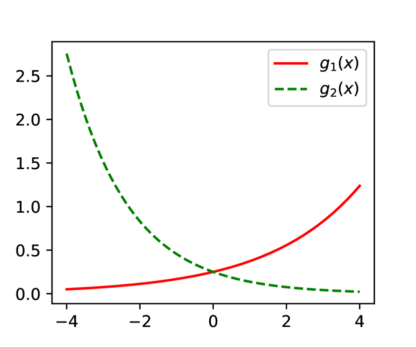
(a) $g_{1}(x)$ and $g_{2}(x)$.

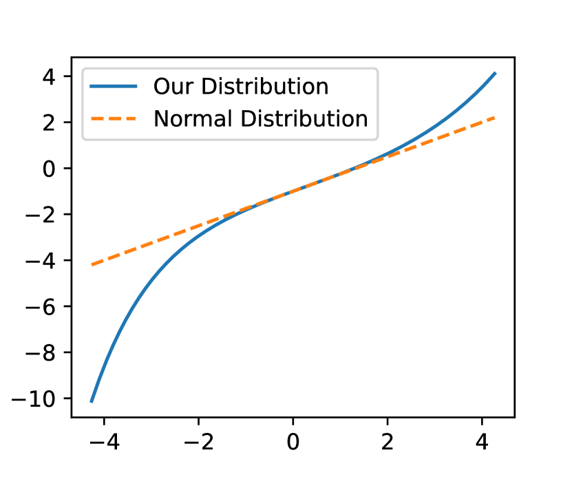
(b) Q-Q plots against standard normal.

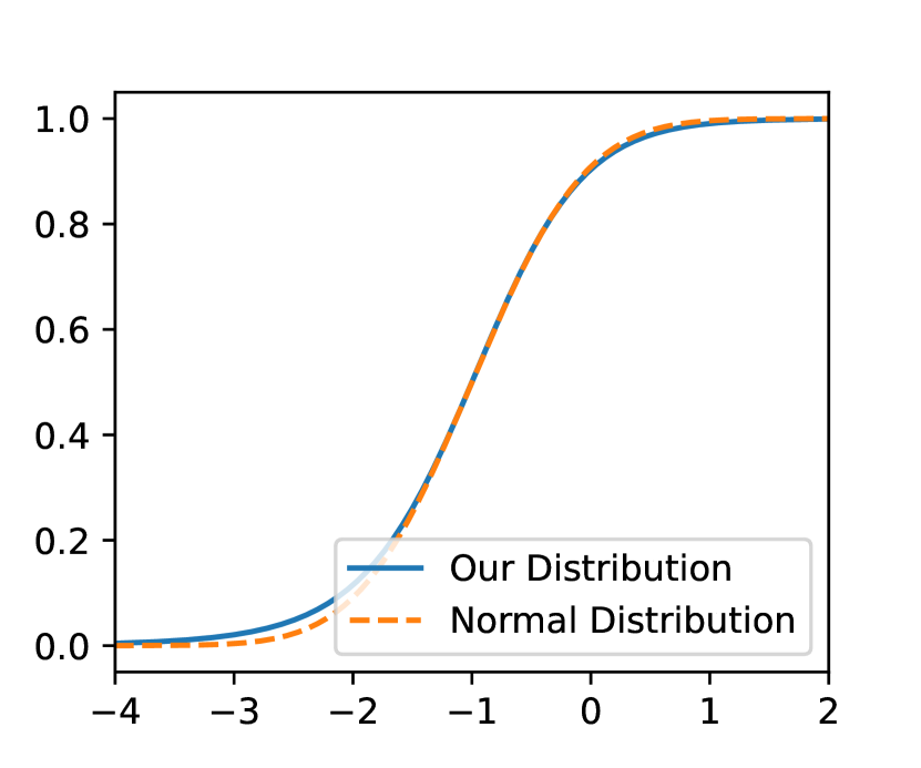
(c) Cumulative functions.

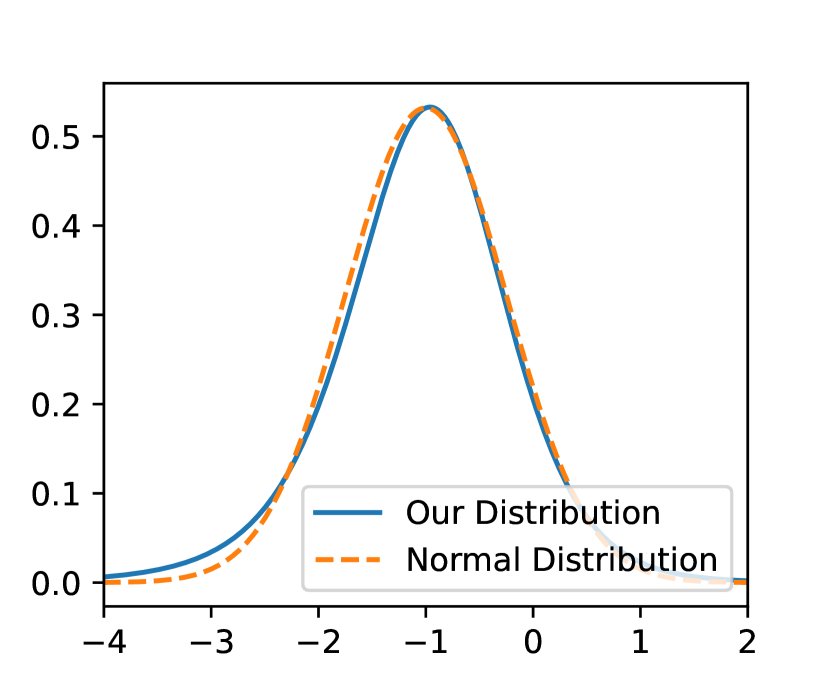
(d) Density functions.

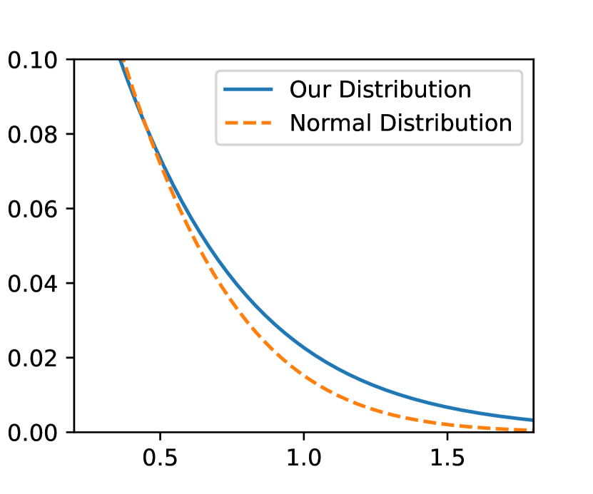
(e) Right-tail densities.

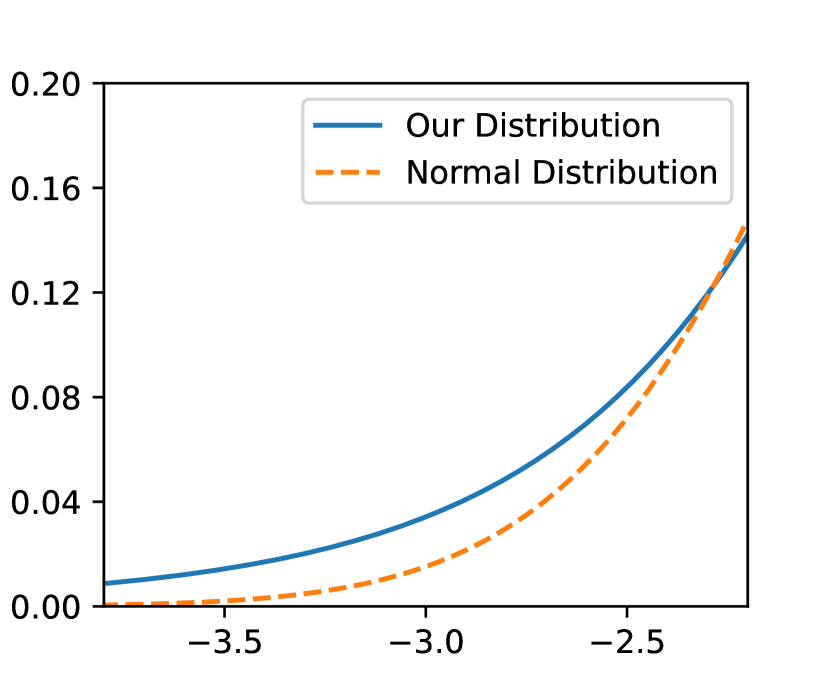
(f) Left-tail densities.

Figure 2: The comparison between the generated distribution determined by the quantile function $f(\Phi^{-1}(\alpha))$ and $\mathcal{N}(\mu,\sigma^{2}(2/A+1)^{2})$, where $f(x)=\mu+\sigma x(u^{x}/A+v^{-x}/A+1)$ with $g_{1}(x)=u^{x}/A$ and $g_{2}(x)=v^{-x}/A$. We set $A=4$, $\mu=-1$, $\sigma=0.5$, $u=1.5$, and $v=1.8$ in this example. The normal distribution is a particular case when $u=v=0$.

To have a distinct comprehension of the proposed transformation, we re-examine the distribution given by Equation (2) or (3). The corresponding transformation $f$ here is $f(x)=\mu+\sigma x(u^{x}/A+v^{-x}/A+1)$ with $g_{1}(x)=u^{x}/A$ and $g_{2}(x)=v^{-x}/A$ shown in Figure 2. We set $A=4$, $\mu=-1$, $\sigma=0.5$, $u=1.5$, and $v=1.8$. It is easy to prove that this $f(x)$ satisfies the four conditions in Proposition 2. Now the new distribution determined by $f(\Phi^{-1}(\alpha))$ has the Q-Q plot against $\Phi^{-1}(\alpha)$ shown in Figure 2, which is exactly the function graph of $f(x)$. We also show the corresponding cumulative function, density function, and tail-side densities in Figure 2. For comparison, we also include a special case of setting $u=v=0$ in $f(x)$ and obtain a normal distribution $\mathcal{N}(\mu,\sigma^{2}(2/A+1)^{2})$. Its results are shown in Figure 2 too. Comparing the tail-side densities of the two distributions, it is intuitive that the new distribution has heavier tails than the normal distribution on both sides.

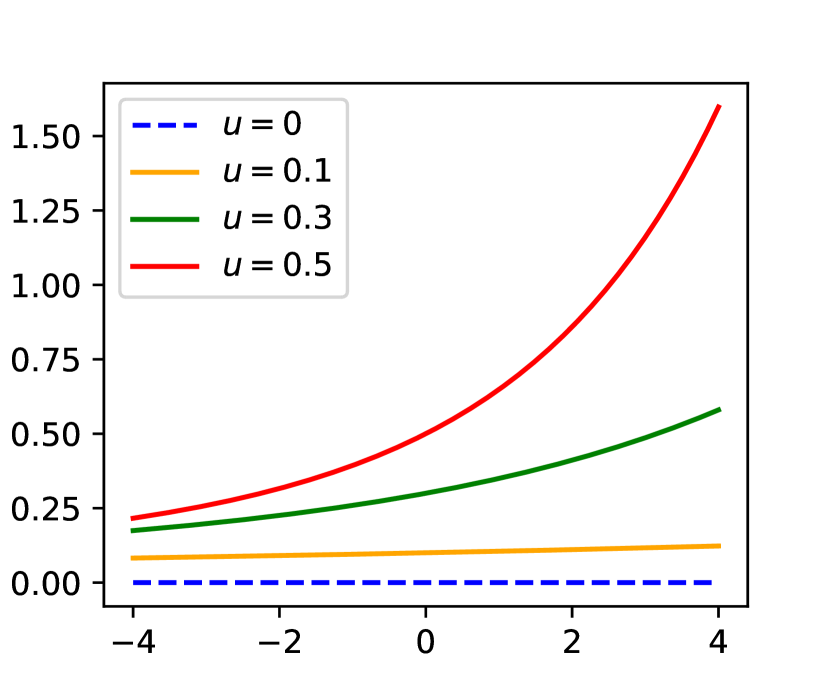
(a) The plots of $g_{1}(x)$.

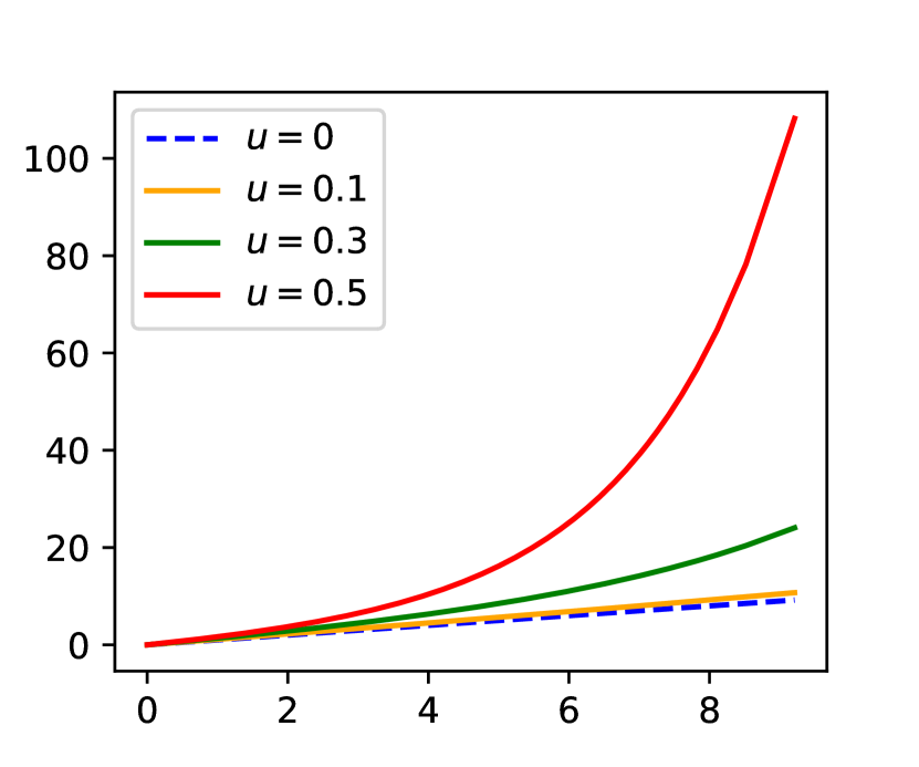
(b) Q-Q plots of the generated distributions against standard exponential.

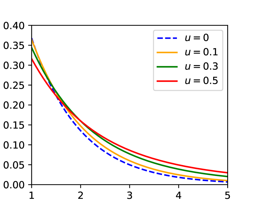
(c) Right-tail densities of the generated distributions.

Figure 3: The comparison among the generated distributions determined by the quantile function $f(F^{-1}(\alpha))$, where $f(x)=x\left((e^{ux}-1)/x+1\right)$ with $g_{1}(x)=(e^{ux}-1)/x$ and $g_{2}(x)=0$. Here $F$ is the cumulative function of standard exponential, and $u$ takes value in $\{0,0.1,0.3,0.5\}$. When $u=0$, we obtain the standard exponential itself.

If one wants to model the arrival of an event, the exponential distribution is the first choice. For this type of distribution whose support is half of $\mathbb{R}$, our framework can be applied too. If the distribution has a positive density on the positive infinite side and our purpose is to make the right tail heavier, we can just set $g_{2}(x)\equiv 0$ and choose an appropriate $g_{1}(x)$ in $f(x)$. In this example, we apply the transformation $f(x)=x\left((e^{ux}-1)/x+1\right)$ to the standard exponential distribution, where $g_{1}(x)=(e^{ux}-1)/x$, and see how it changes the right tail behavior. We set $u=0,0.1,0.3,0.5$ respectively and show the comparison among the generated distributions in Figure 3. One can find that when $g_{1}(x)$ tends to infinity faster, the upper tail of the Q-Q plot against standard exponential becomes heavier, as well as the right tail of the density. This is empirical evidence that the parameter $u$ is a controller of the right tail heaviness of the generated new distribution.

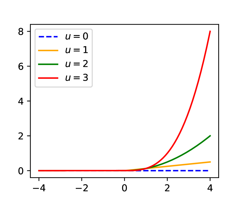
(a) The plots of $g_{1}(x)$.

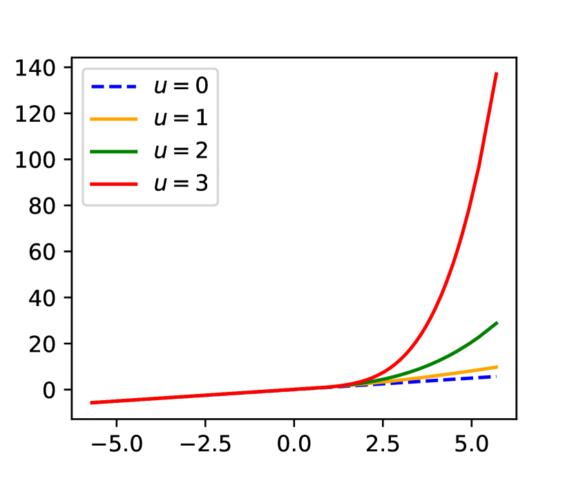
(b) Q-Q plots of the generated distributions against the baseline distribution.

(c) Right-tail densities of the generated distributions.

Figure 4: The comparison among the generated distributions determined by the quantile function $f(F^{-1}(\alpha))$, where $f(x)=x\left(g_{1}(x)+1\right)$ with $g_{1}(x)=\mathbb{I}_{\{x\geq 0\}}\cdot x^{u}/A$. Here $F$ is the cumulative function of the baseline $t$-distribution with 10 degrees of freedom. We set $A=8$, and $u$ takes value in $\{1,2,3\}$. We also add the case of $g_{1}(x)\equiv 0,~{}x\in\mathbb{R}$ into the comparison, i.e., the baseline distribution itself.

The above two examples both incorporate the exponential form for $g_{1}(x)$ or $g_{2}(x)$. We give a third example using power function form. Suppose a $t$-distribution with 10 degrees of freedom is chosen to be the baseline function now, whose cumulative function is denoted as $F(x)$. For symmetry, we only study the effect of $g_{1}(x)$. We set $g_{2}(x)\equiv 0$ and let $g_{1}(x)=x^{u}/A$ for $x\geq 0$ and $g_{1}(x)\equiv 0$ for $x<0$. The transformation $f(x)=x(g_{1}(x)+1)$ is applied on $F^{-1}(\alpha)$, and different values for $u$ from the set $\{1,2,3\}$ are specified. The comparison among the generated new distributions is shown in Figure 4, where the baseline distribution itself is included too, which is the special case when $g_{1}(x)\equiv 0,~{}x\in\mathbb{R}$. From the comparison, we can conclude that the transformation $f$ can yield a new distribution with a heavier tail, whose heaviness is controlled by the parameter $u$. Additional to the empirical analysis here, we rigorously give some theoretical results in the following.

3.2.3 Tail Heaviness

The tail heaviness of the distribution we construct relies on the tail heaviness of the baseline distribution as well as on $g_{1}(x)$ and $g_{2}(x)$ we choose. Due to the similarity, we only need to consider the single side case when $x\to+\infty$ and examine how the asymptotic behavior of $g_{1}(x)$ affects the right tail heaviness of the new distribution because $g_{2}(x)\to 0$. For convenience, we assume the cumulative function of the baseline distribution $F(x)<1$ for any large $x$. We always assume $f(x)$ satisfies the four conditions in Proposition 2. First, we start with some specific cases. All proofs of them are in the appendix.

Proposition 4.

Suppose that the base distribution has the right tail index $\nu$, or equally there exists a positive $\nu$ such that $\lim_{x\to+\infty}x^{\nu}\bar{F}(x)=c>0$. If $\lim_{x\to+\infty}x^{-\nu^{\prime}}g_{1}(x)=c^{\prime}>0$ for some positive $\nu^{\prime}$, then the distribution determined by the quantile function $f(F^{-1}(\alpha))$ has the right tail index $\nu/(1+\nu^{\prime})$. Alternatively, if $\lim_{x\to+\infty}e^{-tx^{\nu^{\prime}}}g_{1}(x)=c^{\prime}>0$ for some $t>0$ and $\nu^{\prime}>0$, then the distribution determined by $f(F^{-1}(\alpha))$ will have a right tail that is as heavy as $(\log x)^{-\nu/\nu^{\prime}}$.

Many distribution families accord with the above description of $F(x)$, such as Student’s $t$ and Pareto distribution. Through the transformation $f$, a new distribution $F(f^{-1}(x))$ with more flexible tails is born. However, there are other commonly-used benchmark distributions such as the normal which satisfies $\lim_{x\to+\infty}xe^{x^{2}/2}\bar{F}(x)=c>0$ and the exponential which satisfies $\lim_{x\to+\infty}e^{tx}\bar{F}(x)=c>0$. For this situation, we have the following statement.

Proposition 5.

(i) Suppose the distribution function $F$ has a Gaussian tail, i.e., $\bar{F}(x)\sim x^{-1}e^{-x^{2}/2}$ as $x\to+\infty$, and we choose a $g_{1}(x)$ satisfying that $g_{1}(x)\sim x^{\nu-1}e^{\nu x^{2}/2}$ for some $\nu>0$ as $x\to+\infty$, then the distribution determined by $f(F^{-1}(\alpha))$ has the tail index $1/\nu$. (ii) Suppose $F$ has a exponential tail, i.e., $\exists t>0$ s.t. $\bar{F}(x)\sim e^{-tx}$ as $x\to+\infty$, and we choose a $g_{1}(x)$ satisfying that $g_{1}(x)\sim x^{-1}e^{\nu x}$ for some $\nu>0$ as $x\to+\infty$, then the distribution determined by $f(F^{-1}(\alpha))$ has the tail index $t/\nu$.

The above are some special cases of the choices for base distribution $F(x)$ and transformation $f(x)$ (especially $g_{1}(x)$). Next, we show two general conclusions about the choices of $F(x)$ and $f(x)$, and the tail heaviness of the new distribution after transformation.

Proposition 6.

Suppose $F$ is the baseline cumulative function and $\lim_{x\to+\infty}g_{1}(x)=+\infty$ in $f(x)$. If $F$ satisfies either one of the following two conditions:
a) $\exists\rho<0$ s.t. $\forall t>0$, $\lim_{x\to+\infty}\bar{F}(tx)/\bar{F}(x)=t^{\rho}$, or equally, $\bar{F}$ is regularly varying but not slowly varying,
b) $\exists t>1$, s.t. $\lim_{x\to+\infty}\bar{F}(tx)/\bar{F}(x)=0$,
then the new distribution determined by the quantile function $f(F^{-1}(\alpha))$ has a heavier right tail than $F$.

Remark 1.

The distribution obtained in Equation (2) or (3) has a heavier right tail than Gaussian, because the cumulative function of Gaussian satisfies Condition b) and $u^{x}/A\to+\infty$. The left-tail side will have a similar conclusion. On the other hand, for any $n\geq 1$, the $n$-th moment of this distribution exists because it is not difficult to verify the existence of $\mathbb{E}[Z^{n}(u^{Z}/A+v^{-Z}/A+1)^{n}]$ when $Z$ is the standard Gaussian. Hence, the tails of this distribution are not so heavy.

Notice that plenty of distributions satisfy either of the two conditions in Proposition 6, and thus this proposition says that for many choices of $F$, any transform $f(x)$ satisfying $g_{1}(x)\to+\infty$ will yield a new distribution with a heavier tail. Furthermore, we state that by choosing appropriate $g_{1}(x)$ and $g_{2}(x)$, our proposed transformation can generate a new distribution $F_{2}$ whose tail is almost arbitrarily heavier than that of the base distribution $F_{1}$.

Proposition 7.

If $F_{1},F_{2}$ are two cumulative functions and $F_{2}$ has a heavier right tail than $F_{1}$, i.e., $\lim_{x\to+\infty}\bar{F_{2}}(x)/\bar{F_{1}}((x-\mu)/\sigma)=+\infty$, $\forall\mu\in\mathbb{R},\sigma>0$. We further assume $F_{2}$ has a decreasing density function $p_{2}$ over large $x$ and $F_{2}^{-1}(\alpha)/F_{1}^{-1}(\alpha)$ is non-decreasing when $\alpha\to 1^{-}$. Then there must exists $g_{1}(x)$ and $g_{2}(x)$ such that $f(x)$ in Equation (5) makes the distribution determined by the quantile function $f(F_{1}^{-1}(\alpha))$ have the same right tail heaviness as $F_{2}$.

Detailed proofs of these propositions are provided in the appendix.

4 Risk-Neural Distribution Extraction

4.1 Problem Setup

To formulate the RND extraction problem, we introduce the following notations. Let $t$ be the present time, i.e., the time at which we observe the market, and $T$ be the time at which the options expire (so $T>t$). We denote the spot price of the underlying security as $S_{t}$ and the price at maturity date as $S_{T}$. The payoff function for a European call option at expiry date $T$ is $V_{C}(S_{T})=\max(S_{T}-K^{C},0)$, where $K^{C}$ is the strike price of the call with the superscript $C$ for call and $P$ for put. The payoff function for a European put is $V_{P}(S_{T})=\max(K^{P}-S_{T},0)$. Cox and Ross (1976) showed that in a market with no-arbitrage, the current equilibrium prices of the European call and put options are given by

$$C_{t} =\tilde{\mathbb{E}}[e^{-r(T-t)}V_{C}(S_{T})]=e^{-r(T-t)}\int_{0}^{+\infty}V_{C}(s_{T})f_{T}(s_{T})ds_{T},$$ (6)

$$P_{t} =\tilde{\mathbb{E}}[e^{-r(T-t)}V_{P}(S_{T})]=e^{-r(T-t)}\int_{0}^{+\infty}V_{P}(s_{T})f_{T}(s_{T})ds_{T},$$

where $\tilde{\mathbb{E}}$ is the risk-neutral expectation and $f_{T}(\cdot)$ is the risk-neutral density function of $S_{T}$. $r$ is the risk-free interest rate. We then denote the log return of the underlying asset as $R_{t:T}\coloneqq\log(S_{T}/S_{t})$, simplified as $R_{\tau}$ where $\tau=T-t$ is the time to maturity. The above Equation (6) can be further written as

$$C_{t} =\tilde{\mathbb{E}}\left[e^{-r\tau}S_{t}\left(e^{R_{\tau}}-\frac{K^{C}}{S_{t}}\right)^{+}\right]=e^{-r\tau}S_{t}\int_{-\infty}^{+\infty}\left(e^{r_{\tau}}-\frac{K^{C}}{S_{t}}\right)^{+}q_{\tau}(r_{\tau})dr_{\tau},$$ (7)

$$P_{t} =\tilde{\mathbb{E}}\left[e^{-r\tau}S_{t}\left(\frac{K^{P}}{S_{t}}-e^{R_{\tau}}\right)^{+}\right]=e^{-r\tau}S_{t}\int_{-\infty}^{+\infty}\left(\frac{K^{P}}{S_{t}}-e^{r_{\tau}}\right)^{+}q_{\tau}(r_{\tau})dr_{\tau},$$

where $(\cdot)^{+}=\max(\cdot,0)$ is the positive part function. $q_{\tau}(\cdot)$ is the risk-neutral density function of $R_{\tau}$. Now consider we have a model for expressing $q_{\tau}(\cdot)$ with unknown parameters that need to be calibrated or learned, and we are given $N=N_{C}+N_{P}$ options ($N_{C}$ calls and $N_{P}$ puts) with observed market prices. The main goal of RND extraction here is to obtain an estimation of $q_{\tau}(\cdot)$ (in any form, such as density function or GML) by minimizing the following objective:

$$\min\frac{1}{N_{C}}\sum_{i=1}^{N_{C}}w_{c_{i}}L(C_{i},\hat{C}_{i})+\frac{1}{N_{P}}\sum_{i=1}^{N_{P}}w_{p_{i}}L(P_{i},\hat{P}_{i}),$$ (8)

where $L(\cdot,\cdot)$ is the loss function (e.g., MSE or relative-type MSE). $\hat{C}_{i}$ and $\hat{P}_{i}$ are option prices estimated by the model, and $C_{i}$ and $P_{i}$ are the option prices observed in the market. And $w_{c_{i}}$ or $w_{p_{i}}$ is a weight that may be related to the liquidity of the option. Or we may choose equal weights for simplicity. Once we have extracted RND, we can price any other path-independent derivatives or further investigate the risk-neutral distributional characteristics or high-order moments which may play an important role in understanding the market’s view of future returns.

4.2 Monte Carlo Pricing with No-Aribtrage Condition

Instead of describing RND with a density function, we set the form of the underlying asset return using the method described in Section 3. Although there are some available model choices in Section 3, we still adopt Equation (3) because it is concise enough, and its effectiveness has been verified before. Therefore, our model for RND extraction is given by

$$R_{\tau}=\mu_{\tau}+\sigma_{\tau}Z\left(\frac{u_{\tau}^{Z}}{A}+\frac{v_{\tau}^{-Z}}{A}+1\right),$$ (9)

where $R_{\tau}$ is the underlying asset return in the risk-neutral world, and $\mu_{\tau}$, $\sigma_{\tau}$, $u_{\tau}$, and $v_{\tau}$ are parameters to be calibrated. For simplicity, we drop the subscript $\tau$ for $\mu,\sigma,u,v$ sometimes in the rest of the paper. We refer to this method as GML, short for generative machine learning.

Given the parameters $\mu,\sigma,u,v$, we can price options with Monte Carlo simulations under the lack of the density for $R_{\tau}$. For European call and put options with contractual parameters (strike prices $K^{C},K^{P}$, the time to maturity $\tau$, interest rate $r$, and underlying price $S_{t}$), we can price them according to Equation (7) by:

$$\hat{C}_{t} =\frac{1}{M}\sum_{m=1}^{M}e^{-r\tau}S_{t}\left(e^{R_{\tau,m}}-\frac{K^{C}}{S_{t}}\right)^{+},$$ (10)

$$\hat{P}_{t} =\frac{1}{M}\sum_{m=1}^{M}e^{-r\tau}S_{t}\left(\frac{K^{P}}{S_{t}}-e^{R_{\tau,m}}\right)^{+},$$

where $R_{\tau,m}$ is the $m$-th i.i.d. realization of $R_{\tau}$:

$$R_{\tau,m} =\mu+\sigma Z_{m}\left(\frac{u^{Z_{m}}}{A}+\frac{v^{-Z_{m}}}{A}+1\right).$$ (11)

$Z_{1},Z_{2},\dots,Z_{M}$ are $M$ i.i.d. realizations of standard Gaussian random variable. This pricing strategy provides a promising approximation than the density-based or integral-based pricing approach when the density function in Equation (7) is sophisticated or cannot be written in an explicit form.

Generally the following condition is to guarantee there is no arbitrage opportunity. When the strike price $K^{C}=0$ for call option, i.e., the payoff is $V_{C}(S_{T})=\max(S_{T}-0,0)=S_{T}$, the call option price should be $S_{t}$. If this condition is expressed in the density form:

$$S_{t}=e^{-r\tau}\int_{0}^{+\infty}s_{T}f_{T}\left(s_{T}\right)ds_{T}=e^{-r\tau}S_{t}\int_{-\infty}^{+\infty}e^{r_{\tau}}q_{\tau}\left(r_{\tau}\right)dr_{\tau},$$ (12)

it would make this condition difficult to satisfy if the density is in a complicated form. However, from Equation (10), this condition in our GML pricing method becomes

$$S_{t} =\frac{1}{M}\sum_{m=1}^{M}e^{-r\tau}S_{t}e^{R_{\tau,m}}.$$ (13)

Obviously, this will imply an equivalent condition that the four RND parameters $\mu,\sigma,u,v$ should satisfy:

$$\mu=r\cdot\tau-\log\left(\frac{1}{M}\sum^{M}_{m=1}e^{\sigma Z_{m}\left(\frac{u^{Z_{m}}}{A}+\frac{v^{-Z_{m}}}{A}+1\right)}\right).$$ (14)

This condition informs us that we only need to calibrate the there parameters $\sigma,u,v$ when extracting RND from option prices, and the remaining parameter $\mu$ would be hereafter determined by the above no-arbitrage condition.

4.2.1 Cross-Maturity Arbitrage

An option’s value will decline over time. Or equivalently, the longer the time-to-maturity $\tau$, the greater the option value. Mathematically, the partial derivative of the option value with respect to $\tau$ should be positive. Or, there will be arbitrage opportunity existing. This requires that the RNDs for different $\tau$ satisfy some constraint.

To address it, we may need to calibrate the RNDs for different $\tau$ together, for example, 1 month, 3 months, 6 months, 1 year, and so on. Given the fact that the option prices quoted in the market are monotonically increasing with respect to $\tau$ almost all the time, we thereby take a simpler approach of post-processing here. Firstly, we separately calibrate the RNDs for different $\tau$. Then, we examine if the cross-maturity arbitrage is absent, or, if the option values priced with our RNDs are monotonically increasing with those $\tau$. If not, we tune or adjust the RND parameters $\sigma_{\tau},u_{\tau},v_{\tau}$ ($\mu_{\tau}$ is determined by them) with a slight amount, to eliminate the cross-maturity arbitrage. More specifically, we increase $\sigma_{\tau_{2}}$ slightly when the extracted RND at $\tau_{2}$ yields smaller option values than the RND at $\tau_{1}$ does, when $\tau_{2}>\tau_{1}$.

Indeed, in our numerical studies, separately calibrating the RNDs for different $\tau$ does not result in the violation of the cross-maturity arbitrage constraint. In other words, the post-processing does not happen even once in our experimental studies. However, the interpolation of RNDs for all $\tau\in[0,\mathcal{T}]$ will be a difficult task, and is out of the scope of this paper.

4.3 Calibration of GML Model

In this paper, we only consider calibrating from European option prices. Calibration is always a critical problem which aims to minimize the gap between estimated prices and real option prices. Suppose we can obtain market prices of $N_{C}$ call options with strikes $K^{C}_{i}$, $i=1,\dots,N_{C}$ and $N_{P}$ put options with strikes $K^{P}_{i}$, $i=1,\dots,N_{P}$ with the same maturity time, denoted as $C_{i}$ and $P_{i}$. We minimize the following relative loss between the prices generated by the GML model and the real prices:

$$\min_{\sigma,u,v}L=\frac{1}{N_{C}}\sum_{i=1}^{N_{C}}(\hat{C}_{i}/C_{i}-1)^{2}+\frac{1}{N_{P}}\sum_{i=1}^{N_{P}}(\hat{P}_{i}/P_{i}-1)^{2},$$ (15)

where $\hat{C_{i}},\hat{P_{i}}$ are the estimated prices using our GML model, see Equation (10).

To be more specific, we have designed a detailed algorithm to calibrate our model parameters. Firstly, we fix a random seed to simulate $M=1,000,000$ samples $Z_{m}$ from standard Gaussian distribution and initialize the three parameters as $\sigma=0.2,u=v=1.1$, followed by Equation (14) to compute the parameter $\mu$. Then we use Equation (11) to compute the simulated log-return $R_{\tau,m}$, and compute the estimated option prices by Equation (10). The relative mean square error loss $L$ (abbreviated as RLOS) in Equation (15) is then optimized by Adam optimizer (Kingma and Ba, 2014) in PyTorch (Paszke et al., 2019) with the learning rate $\gamma=0.1$ in every gradient descent step. These steps will be run until the loss no longer decreases with some criteria, called the early-stopping strategy. The algorithm will return to us the calibrated parameters $\sigma$, $u$, $v$, and $\mu$. And we now can express the risk-neutral distribution by Equation (9) and can evaluate any distributional characteristics of it. We summarize the calibration algorithm details in Algorithm 1.

After the successful calibration of our model, it can be applied for various purposes. For instance, it can be used to validate research hypotheses empirically, analyze market expectations, invest and hedge, and price other derivatives. The main advantage of our proposed pricing procedure is that it offers flexibility in capturing different degrees of tailedness in log-return distribution, by succinctly adjusting tail parameters $u$ and $v$. Additionally, our model is convenient for sampling, and easy for computing density values numerically (derived from the quantile function). So, it is beneficial for various numerical purposes.

Algorithm 1 Risk-neutral distribution extraction using the parsimonious GML model.

0:   $S_{t}$: the current price of the underlying asset at time $t$; $\tau=T-t$: the time to maturity of options;$r$: the risk-free interest rate between $t$ and $T$;$C_{i},~{}K_{i}^{C},~{}i=1,\dots,N_{C}$: observed market prices and strikes of European call options at time $t$;$P_{i},~{}K_{i}^{P},~{}i=1,\dots,N_{P}$: observed market prices and strikes of European put options at time $t$; $A$: a hyper-parameter in risk-neutral distribution of the log-return (by default $A=4$).

0:  parameters $\mu$, $\sigma$, $u$, $v$ of the risk-neutral distribution of the log-return $R_{\tau}=\log(S_{T}/S_{t})$.

1:  Initialize $\sigma=0.2,~{}u=1.1,~{}v=1.1$ and sample $Z_{m}\sim\mathcal{N}(0,1)$, $m=1,\dots,M$.

2:  repeat

3:     Compute $Q_{m}\leftarrow\sigma\cdot Z_{m}\cdot(\frac{u^{Z_{m}}}{A}+\frac{v^{-Z_{m}}}{A}+1)$ and $\mu\leftarrow r\cdot\tau-\log(\frac{1}{M}\sum^{M}_{m=1}e^{Q_{m}})$;

4:     Compute simulated log-return $R_{\tau,m}\leftarrow\mu+Q_{m}$, $m=1,\dots,M$;

5:     Calculate call and put option prices with simulation-based averages in risk-neutral world:

$$\hat{C}_{i} \leftarrow S_{t}\cdot e^{-r\tau}\cdot\frac{1}{M}\sum^{M}_{m=1}\left(e^{R_{\tau,m}}-\frac{K_{i}^{C}}{S_{t}}\right)^{+},~{}i=1,\dots,N_{C};$$

$$\hat{P}_{i} \leftarrow S_{t}\cdot e^{-r\tau}\cdot\frac{1}{M}\sum^{M}_{m=1}\left(\frac{K_{i}^{P}}{S_{t}}-e^{R_{\tau,m}}\right)^{+},~{}i=1,\dots,N_{P};$$

6:     Obtain loss function $L=\frac{1}{N_{C}}\sum^{N_{C}}_{i=1}(\hat{C}_{i}/C_{i}-1)^{2}+\frac{1}{N_{P}}\sum^{N_{P}}_{i=1}(\hat{P}_{i}/P_{i}-1)^{2}$;

7:     Update $\sigma,u,v$ with the gradient descent:

$$\sigma\leftarrow\sigma-\gamma\frac{\partial L}{\partial\sigma},~{}~{}u\leftarrow u-\gamma\frac{\partial L}{\partial u},~{}~{}v\leftarrow v-\gamma\frac{\partial L}{\partial v},$$

where $\gamma$ is the step size;

8:  until the loss no longer decreases with some criteria.

9:  Compute $Q_{m}$ again and set $\mu\leftarrow r\cdot\tau-\log(\frac{1}{M}\sum^{M}_{m=1}e^{Q_{m}})$.

10:  return  $\mu,\sigma,u,v$.

5 Experimental Studies

In this section, we present a comprehensive evaluation of the proposed GML method through both simulation and empirical studies. Our studies comprise two parts. Firstly, we conduct experiments in simulated markets to assess the model’s performance. Secondly, we compare our method to three existing parametric methods in real financial markets and investigate the high-order moments of the extracted RNDs. These studies provide compelling evidence for the effectiveness and accuracy of the proposed GML method in capturing the risk-neutral distribution and its detailed characteristics.

5.1 Simulation Experiments

5.1.1 Self-Calibration with GML Option Prices

Option pricing in Equation (10) using the GML model can be regarded as a forward computation process that requires model parameters ($\mu,\sigma,u,v$, noted that $\mu$ is determined by the other three parameters) and contractual inputs (e.g., underlying price $S_{t}$, strike price $K$, time to maturity $\tau$, etc.). On the other hand, calibration is a backward computation process that involves searching for optimal model parameters by minimizing the error between the estimated and the observed option prices. In the first part of our simulation study, we aim to examine the parameter accuracy in self-calibration, i.e., calibrating from the prices generated by Equation (10). Specifically, we firstly generate multiple call and put option prices using Equation (10) with true parameters falling in rational ranges ($\sigma\in\{0.1,0.2,0.3,0.4,0.5\}$ and $u,v\in\{1.0,1.1,1.2,1.3,1.4,1.5,1.6\}$). The contractual parameters $S_{t}=50$, $r=0.015$, $\tau=0.5$, and $K\in[30,70]$ spreading over the interval with an increment of 5. Secondly, these option prices would serve as the observed prices and the calibration is conducted using Algorithm 1. Eventually we evaluate the performance with the mean absolute error (MAE) between the calibrated parameters ($\hat{\sigma},\hat{u},\hat{v},\hat{\mu}$) and the true ones ($\sigma,u,v,\mu$). The results of this study will provide evidence of the accuracy of our model’s calibration process, or more specifically, the effectiveness of Algorithm 1.

Table 1: Self-calibration MAE statistics for all settings of $u,v\in\{1.0,1.1,1.2,1.3,1.4,1.5,1.6\}$ when $\sigma$ is fixed to be $0.1,0.2,0.3,0.4,0.5$ respectively. The MAE measures the error between the calibrated parameters ($\hat{\sigma},\hat{u},\hat{v},\hat{\mu}$) and the true ones.

$\boldsymbol{\sigma}$		0.10	0.20	0.30	0.40	0.50
MAE	Minimum	0.0000	0.0000	0.0000	0.0000	0.0000
	Mean	0.0050	0.0143	0.0120	0.0211	0.0626
	Maximum	0.3000	0.4000	0.3300	0.3700	0.3000

In Table 1, we report the minimum, mean, and maximum MAE between the true and the calibrated parameters across various settings of $u$ and $v$ when $\sigma$ is fixed. It is not surprising to see that our calibration process performs well under different values of $\sigma$. The fact that we achieve zero minimum MAE for all values of $\sigma$ suggests that our model is robust and reliable. The mean MAE and maximum MAE are also relatively low, indicating that our calibration process is able to accurately estimate the model parameters. Overall, our simulation study provides evidence that the self-calibration is accurate or the algorithm is effective. This is an important step in developing a reliable and practical method that can be used in real-world applications.

5.1.2 Calibration with Heston Option Prices

The Heston model, which incorporates stochastic volatility, is a classical and vital option pricing model in financial derivatives world (Heston, 1993). In the second part of our simulation experiments, we aim to evaluate the effectiveness of our model in fitting Heston model prices, or equivalently, in extracting RNDs determined by the Heston model. We select a rational set of Heston model parameters, including an initial variance $v_{0}$, a mean reversion rate $\kappa$, a long-term mean of volatility $\theta$, a volatility of volatility $\xi$, and a correlation $\rho$ between the two Brownian motions. Three model choices are considered: $\{v_{0}=0.04,\kappa=0.15,\theta=0.15,\xi=0.5,\rho=-0.7\}$, $\{v_{0}=0.04,\kappa=0.6,\theta=0.2,\xi=0.15,\rho=-0.8\}$, and $\{v_{0}=0.04,\kappa=0.9,\theta=0.2,\xi=0.15,\rho=0.8\}$. The contractual parameters are identical to those in Section 5.1.1. Nine call contracts and nine put contracts are used with an underlying stock price $S_{t}=50$, with the same strikes ranging from 30 to 70 with an increment of 5. The time to maturity $\tau=0.5$ and the risk-free rate $r=0.015$. We calibrate our model using Algorithm 1 with these Heston option prices which serve as observed market prices, and compare the calibrated model to the true one on both RNDs and the implied volatility curves they generate.

Figure 5: Comparisons between the true Heston RND/implied volatility curve and the calibrated ones by our model GML. MAE between the two implied volatility curves is displayed as well.

We plot the RNDs/implied volatility curves generated by the Heston model and our calibrated model GML in Figure 5, with MAE between the two implied volatility curves displayed as well. It is shown that GML has the capability to capture the main shape of Heston implied volatility curve with sufficiently low MAE. We can also observe that GML can capture the tail-side shape when the strike price $K$ is far from the underlying stock price $S_{t}$. Figure 5 also depicts the true Heston density and the recovered density generated by our model. It can be observed that the true and recovered densities are much close, sometimes almost identical. Besides, our model achieves a close fit in the tails of the distribution. These results are indicative of the effectiveness of our proposed method in extracting the various risk-neutral densities.

5.2 Empirical Results in Real Financial Markets

In this part, we present an empirical experiment to assess the effectiveness of our proposed GML method in real financial markets by comparing the fitting performance to some classical parametric models’ performance, namely the double log-normal model (DLN) (Bahra, 1996), generalized beta model (GB) (Bookstaber and McDonald, 1987), and Edgeworth expansion method (EW) (Jarrow and Rudd, 1982). We use all of them to extract risk-neutral densities in four years’ real market data.

Table 2: Average relative losses achieved in the calibrations of our proposed GML method and of the three parametric competitors. The lowest loss is displayed in bold. All models here have very few parameters that need to be calibrated, hence are unlikely to be overfitted.

Year	Relative Loss	GML (Ours)	DLN	GB	EW
2006	RLOS0	2.91	2.91	60.18	188.05
	RLOS14	0.42	0.42	5.47	7.32
	RLOS365	4.11	4.14	80.44	271.82
2007	RLOS0	5.51	5.58	186.32	543.40
	RLOS14	0.24	0.33	25.63	55.21
	RLOS365	7.10	7.20	241.54	704.92
2008	RLOS0	0.99	22.84	730.33	1451.99
	RLOS14	0.25	0.70	176.62	87.24
	RLOS365	1.20	28.71	913.58	1829.86
2009	RLOS0	0.84	2.20	115.60	319.96
	RLOS14	0.41	0.54	72.88	22.82
	RLOS365	1.00	2.62	130.68	400.45

Table 3: MAE between the estimated and the market-observed implied volatility curves (days-to-maturity $d\leq$ 365). The lowest MAE is in bold.

Year	GML (Ours)	DLN	GB	EW
2006	0.1686	0.4833	0.6344	1.1016
2007	0.1102	0.2579	0.3007	0.5924
2008	0.1620	0.1647	0.2858	0.4525
2009	0.4181	0.3714	0.5513	0.8789

5.2.1 Data Description

We only focus on European options in this paper. We select the data of European option contracts on S&P 500 index that come from OptionMetrics IvyDB US database through the Wharton Research Data Services, which provides end-of-day bid and ask quotes for the underlying stock index and option contracts. The data samples we select cover the period from January 2, 2006 to December 31, 2009, in total of four years. The occurrence of the worldwide financial crisis in the year 2008 may present an opportunity to test our model’s stability in extreme market conditions. Prior to calibration, several pre-processing procedures are implemented. The midpoint price between the bid and ask is used as the daily price of the underlying S&P 500 index (denoted as $S_{t}$). The same average operation is performed on the daily call and put option prices. Time-to-maturity $\tau$ is normalized on an annual basis, i.e., $\tau=\text{days-to-maturity}/365$. The risk-free rate $r$ is linearly interpolated to match the time-to-maturity of the corresponding option. The dataset comprises 12,968 option contracts in total.

Figure 6: Some implied volatility curves generated by the calibrated GML model and observed in the market, on selected dates and time-to-maturities in the year 2006. The MAE between them is displayed as well.

Figure 7: Some implied volatility curves generated by the calibrated GML model and observed in the market, on selected dates and time-to-maturities in the year 2007. The MAE between them is displayed as well.

5.2.2 Calibration with Empirical Data

We design our empirical experiment as follows. We train the GML model and obtain the calibrated parameters $\hat{\mu},\hat{\sigma},\hat{u},\hat{v}$ for each option maturity by Algorithm 1. We then evaluate our model’s performance using the relative mean square error (relative loss, or RLOS) between the estimated and the observed prices in Equation (15) as our metric, which is the optimization objective of the calibration. We compare the proposed method with three classical parametric methods for RND extraction, which are DLN, GB, and EW. We calibrate these models’ parameters respectively with the R package RND (Hamidieh, 2017). The results are shown in Table 2, in which we report the relative loss averaged annually and consider the options in three groups respectively. According to the days-to-maturity $d$, the three groups are: $d\geq 0$ (all options), $d\geq 14$ (greater than two weeks), and $d\leq 365$ (less than one year), which are symbolized with the subscript $0,14,365$ respectively. We design these categories since some of the options may have fluctuating prices when approaching the expiry or are much illiquid when they are far from expiry.

It is important to note that all models here have very few parameters that need to be calibrated, hence are unlikely to be overfitted. Overall, the GML model outperforms the other three competitors with lower relative losses in all the three days-to-maturity categories in every year of the four. The GB and EW methods for extracting the risk-neutral density sometimes perform poorly, yielding at least ten times the loss of our model or DLN. In the financial crisis year of 2008, our model even achieves superior performance, while the DLN model’s loss increases dramatically in that year. These results demonstrate the effectiveness of the GML model and the algorithm in extracting the risk-neutral density from real financial market data, even under extreme market conditions.

5.2.3 Implied Volatility Curves

We continue to assess the performance of all models by comparing the implied volatility curve generated by the model to that observed in the market. To do so, we adopt the mean absolute error (MAE) as our evaluation metric between the market curve and the estimated curve generated by the model. Specifically, we focus on options with days-to-maturity $d$ less than or equal to 365, as these options are more frequently and actively traded. Moreover, when computing the implied volatility curves and plotting them, we only use out-of-the-money (OTM) options because they are typically preferred by investors and they are less costly relative to in-the-money (ITM) options. We may observe a discontinuity around the underlying asset price $S_{t}$ in the implied volatility curve of the market, as it is constructed by combining the OTM call curve and the OTM put curve. To obtain a well-behaved curve with a satisfying shape, further smoothing techniques can be applied. However, we have omitted these smoothing steps in our analysis, as our goal is to focus on the fitting accuracy of the GML model and others.

The annual average MAE results are summarized in Table 3. We observe that our model GML mostly outperforms the three parametric baseline methods with significantly low levels of MAE. Additionally, we note that DLN achieves superior performance among these three baselines. Figure 6 and 7 depict the implied volatility curves on selected dates and days-to-maturities, where we plot the market curves in blue and the curves after the calibration of GML in orange. The results reveal that the proposed GML method achieves good fitness to the market implied volatility curves, with low MAE shown in the figure legend. GML does particularly well in capturing the tails where the strike prices are significantly lower or higher than the underlying price.

5.2.4 Skewness and Kurtosis of RNDs

Table 4: Five empirical quantiles of skewness and excess kurtosis of the extracted RNDs of log-return $R_{\tau}=\log(S_{T}/S_{t})$. $q_{\alpha}$ denotes the quantile of level $\alpha\%$.

Year	Days-to-Maturity	Skewness					Kurtosis
		$q_{05}$	$q_{25}$	$q_{50}$	$q_{75}$	$q_{95}$	$q_{05}$	$q_{25}$	$q_{50}$	$q_{75}$	$q_{95}$
2006	$d>0$	-6.19	-3.00	-1.94	-0.33	-0.02	0.02	0.40	13.47	34.40	156.54
	$d\geq 14$	-6.47	-3.20	-2.18	-0.41	-0.05	0.03	0.60	17.26	39.33	171.54
	$d\leq 365$	-3.73	-2.48	-1.52	-0.34	0.01	0.02	0.43	7.97	22.76	54.75
2007	$d>0$	-29.30	-5.97	-2.80	-0.59	0.02	0.02	1.17	29.60	145.27	2975.45
	$d\geq 14$	-31.02	-6.81	-3.15	-1.33	-0.01	0.02	6.04	38.26	189.46	3294.10
	$d\leq 365$	-32.05	-5.27	-2.49	-0.43	0.03	0.01	0.64	23.05	112.69	3491.08
2008	$d>0$	-52.17	-5.13	-0.31	-0.17	-0.07	0.06	0.14	0.38	107.29	8195.12
	$d\geq 14$	-54.07	-6.78	-0.31	-0.17	-0.08	0.07	0.14	0.37	188.42	8719.74
	$d\leq 365$	-46.34	-1.24	-0.28	-0.17	-0.07	0.06	0.15	0.31	5.25	6672.97
2009	$d>0$	-26.43	-0.90	-0.20	-0.12	-0.06	0.06	0.09	0.18	2.70	2477.36
	$d\geq 14$	-29.83	-1.56	-0.19	-0.12	-0.07	0.06	0.09	0.17	8.52	3088.18
	$d\leq 365$	-2.73	-0.35	-0.18	-0.12	-0.06	0.06	0.10	0.16	0.45	28.28

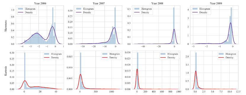
Figure 8: Histograms of skewness and excess kurtosis of the extracted RNDs of log-return $R_{\tau}=\log(S_{T}/S_{t})$.

In this part, we desire to investigate the skewness and kurtosis of the risk-neutral densities (RNDs) extracted by our model. We aim for their distributional characteristics in each year. Note that we have already calibrated the model for each date and days-to-maturity and obtained three required parameters $\hat{\sigma},\hat{u},\hat{v}$ which could fully determine the risk-neutral density. To compute its (empirical) skewness and kurtosis, we draw a sufficiently large set of samples with $M=1,000,000$ from the standard Gaussian distribution and transform them with calibrated parameters $\hat{\sigma},\hat{u},\hat{v}$ and Equation (11) to obtain samples drawn from the estimated RND. Similar to the processing in the selection of days-to-maturity $d$ in Table 2, we categorize the options using three time ranges ($d>0$, $d\geq 14$, and $d\leq 365$). In each time range, we investigate the distributions of skewness and excess kurtosis in all risk-neutral densities by computing their five empirical quantiles of levels 5%, 25%, 50%, 75%, and 95%.

We can observe from Table 4 that the risk-neutral distribution of log-return $\log(S_{T}/S_{t})$ was left-skewed with a negative value of skewness in most times. It became more negative in the year 2007 and reached a spike in the year 2008 with extremely large (excess) kurtosis as well. It returned to normal in the year 2009 when we restrict $d\leq 365$. As to the kurtosis, it was similar that it reached the spike in 2008 and dropped back in 2009. These observations are consistent with the histograms of skewness and kurtosis of the densities in every year, as displayed in Figure 8.

6 Conclusions

In this paper, we propose to use a new parametric method to extract risk-neutral density of the asset return, which is a type of parsimonious generative machine learning. It has a flexible design with a succinct mathematical form, which can effectively learn asymmetric non-Gaussian tails in the data. We then derive the arbitrage-free conditions it should satisfy in pricing. We also design a Monte Carlo algorithm for calibrating the parameters. With the help of modern machine learning computing tools (such as PyTorch and Adam), the algorithm works well on various calibration tasks, as illustrate in the experiments.

We demonstrate the effectiveness of our approach in both self-calibration and fitting Heston option prices in simulation experiments. In real-data empirical studies, we achieve superior calibration results with lower relative losses compared to three classical parametric baselines. We obtain low MAE most of the time when modeling the implied volatility curves and show that our model can capture the main shape and tails of the curve. We proceed to investigate the skewness and kurtosis of RNDs extracted by our model. The results are highly intuitive, such as the kurtosis spike and the skewness spike during the financial crisis in 2008. Overall, our proposed approach offers a powerful and flexible framework for modeling risk-neutral density and it may have further potential applications for both researchers and practitioners.

More generally, the proposed methodology is widely applicable in data fitting and probabilistic forecasting. It is more practical than many existing methods. The parameter estimation or learning given the dataset can be done via maximum likelihood or quantile regression.

Appendix A Some Proofs

In this appendix, we provide some proofs of those propositions proposed in this work.

For Proposition 4:

Proof.

The cumulative distribution function of $f(F^{-1}(\alpha))$ is $F(f^{-1}(x))$. We have

$$\lim_{x\to+\infty}x^{\frac{\nu}{1+\nu^{\prime}}}\left(1-F(f^{-1}(x))\right)= \lim_{x\to+\infty}f(x)^{\frac{\nu}{1+\nu^{\prime}}}\bar{F}(x)=\lim_{x\to+\infty}c\left(\frac{f(x)}{x}\right)^{\frac{\nu}{1+\nu^{\prime}}}x^{\frac{-\nu\nu^{\prime}}{1+\nu^{\prime}}}$$

$$= \lim_{x\to+\infty}c\left(\frac{\frac{\mu}{x}+\sigma(g_{1}(x)+g_{2}(x)+1)}{x^{\nu^{\prime}}}\right)^{\frac{\nu}{1+\nu^{\prime}}}=c(\sigma c^{\prime})^{\frac{\nu}{1+\nu^{\prime}}}.$$

Alternatively,

$$\lim_{x\to+\infty}(\log x)^{\frac{\nu}{\nu^{\prime}}}\left(1-F(f^{-1}(x))\right)=\lim_{x\to+\infty}(\log f(x))^{\frac{\nu}{\nu^{\prime}}}\bar{F}(x)$$

$$= \lim_{x\to+\infty}c\left(\log\frac{f(x)}{x}+\log x\right)^{\frac{\nu}{\nu^{\prime}}}x^{-\nu}=\lim_{x\to+\infty}c\left(\frac{\log(\sigma c^{\prime})+tx^{\nu^{\prime}}+\log x}{x^{\nu^{\prime}}}\right)^{\frac{\nu}{\nu^{\prime}}}=ct^{\frac{\nu}{\nu^{\prime}}}.$$

∎

For Proposition 5:

Proof.

For (i),

$$\lim_{x\to+\infty}x^{\frac{1}{\nu}}\left(1-F(f^{-1}(x))\right)= \lim_{x\to+\infty}f(x)^{\frac{1}{\nu}}\bar{F}(x)=\lim_{x\to+\infty}c\left(\frac{f(x)}{\sigma xg_{1}(x)}\right)^{\frac{1}{\nu}}\frac{\left(\sigma xg_{1}(x)\right)^{\frac{1}{\nu}}}{xe^{x^{2}/2}}$$

$$= \lim_{x\to+\infty}c(\sigma c^{\prime})^{\frac{1}{\nu}}\frac{\left(xx^{\nu-1}e^{\nu x^{2}/2}\right)^{\frac{1}{\nu}}}{xe^{x^{2}/2}}=c(\sigma c^{\prime})^{\frac{1}{\nu}},$$

where $c$ and $c^{\prime}$ are the corresponding constants. For (ii),

$$\lim_{x\to+\infty}x^{\frac{t}{\nu}}\left(1-F(f^{-1}(x))\right)= \lim_{x\to+\infty}f(x)^{\frac{t}{\nu}}\bar{F}(x)=\lim_{x\to+\infty}c\left(\frac{f(x)}{\sigma xg_{1}(x)}\right)^{\frac{t}{\nu}}\frac{(\sigma xg_{1}(x))^{\frac{t}{\nu}}}{e^{tx}}$$

$$= \lim_{x\to+\infty}c(\sigma c^{\prime})^{\frac{t}{\nu}}\frac{(xx^{-1}e^{\nu x})^{\frac{t}{\nu}}}{e^{tx}}=c(\sigma c^{\prime})^{\frac{t}{\nu}}.$$

∎

For Proposition 6:

Proof.

We will prove the following limit is $+\infty$ for any $\mu\in\mathbb{R}$ and $\sigma>0$:

$$\lim_{x\to+\infty}\frac{1-F(f^{-1}(x))}{1-F(\frac{x-\mu}{\sigma})}=\lim_{x\to+\infty}\frac{\bar{F}(x)}{\bar{F}(\frac{f(x)-\mu}{\sigma})}.$$

Because there are also arbitrary $\mu$ and $\sigma$ in the formulation of $f(x)$, they are merged and the above limit becomes $\lim_{x\to+\infty}\bar{F}(x)/\bar{F}(f(x))$. Because $\lim_{x\to+\infty}f(x)/x=\lim_{x\to+\infty}\sigma(g_{1}(x)+1)=+\infty$, so for any large $t$, when $x$ is large enough we have $f(x)>tx$. When the condition a) holds,

$$\frac{\bar{F}(x)}{\bar{F}(f(x))}\geq\frac{\bar{F}(x)}{\bar{F}(tx)}\to t^{-\rho},\quad x\to+\infty.$$

Thus $\bar{F}(x)/\bar{F}(f(x))\geq\bar{F}(x)/\bar{F}(tx)\geq t^{-\rho}-1$ for large enough $x$. From the arbitrariness of $t$, we obtain $\lim_{x\to+\infty}\bar{F}(x)/\bar{F}(f(x))=+\infty$. When the condition b) holds, for the fixed $t>1$ and any large $x$,

$$\frac{\bar{F}(x)}{\bar{F}(f(x))}\geq\frac{\bar{F}(x)}{\bar{F}(tx)}\to+\infty,\quad x\to+\infty.$$

Hence our proof is completed. ∎

For Proposition 7:

Proof.

We first prove that when $x\to+\infty$, $F_{2}^{-1}(F_{1}(x))/x\to+\infty$, which is equivalent to $\lim_{\alpha\to 1^{-}}F_{2}^{-1}(\alpha)/F_{1}^{-1}(\alpha)=+\infty$. If not, there must exists $M>0$ and a sequence $x_{i}\to+\infty$ such that $F_{2}^{-1}(F_{1}(x_{i}))\leq Mx_{i}$. So, $F_{1}(x_{i})\leq F_{2}(Mx_{i})$ and $\bar{F_{1}}(x_{i})\geq\bar{F_{2}}(Mx_{i})$, which is contradictory to $\bar{F_{2}}(Mx)/\bar{F_{1}}(x)\to+\infty$. Additionally, $F_{2}^{-1}(F_{1}(x))/x$ is non-decreasing obviously for large $x$.

We set $g_{1}(x)=\left(-\mu+F_{2}^{-1}(F_{1}(x))\right)/(\sigma x)-1$ for large $x$, where $\mu$ and $\sigma$ are any chosen parameters in the formulation of $f(x)$. So $g_{1}(x)\to+\infty$ as $x\to+\infty$. We further set $g_{2}(x)$ to be a quickly decaying function satisfying $\lim_{x\to+\infty}xg_{2}(x)=0$ and $\lim_{x\to+\infty}xg_{2}(x)\cdot p_{2}(h(x))/\bar{F_{2}}(h(x))=0$, where $h(x)=F_{2}^{-1}(F_{1}(x))$ (e.g., we can set $g_{2}(x)\equiv 0$ for large $x$). It is not difficult to let $g_{1}(x)$ and $g_{2}(x)$ satisfy all the conditions in Proposition 2. Now,

$$\lim_{x\to+\infty}\frac{1-F_{2}(x)}{1-F_{1}(f^{-1}(x))}= \lim_{x\to+\infty}\frac{\bar{F_{2}}(f(x))}{\bar{F_{1}}(x)}=\lim_{x\to+\infty}\frac{\bar{F_{2}}\left(\sigma xg_{2}(x)+h(x)\right)}{\bar{F_{1}}(x)}.$$

Apply the mean value theorem and notice that $\bar{F_{2}}(h(x))=\bar{F_{1}}(x)$,

$$\frac{\bar{F_{2}}\left(\sigma xg_{2}(x)+h(x)\right)}{\bar{F_{1}}(x)}=\frac{\bar{F_{2}}(h(x))-p_{2}(\xi_{x})\sigma xg_{2}(x)}{\bar{F_{2}}(h(x))}=1-\sigma xg_{2}(x)\frac{p_{2}(\xi_{x})}{\bar{F_{2}}(h(x))}\to 1,$$

$$\text{because }\sigma xg_{2}(x)\frac{p_{2}(\xi_{x})}{\bar{F_{2}}(h(x))}\leq\sigma xg_{2}(x)\frac{p_{2}(h(x))}{\bar{F_{2}}(h(x))}\to 0,\quad\text{as }x\to+\infty.$$

So, $\lim_{x\to+\infty}\left(1-F_{2}(x)\right)/\left(1-F_{1}(f^{-1}(x))\right)=1$. ∎

References

- Abadir and Rockinger (2003) Abadir, K.M., Rockinger, M., 2003. Density functionals, with an option-pricing application. Econometric Theory 19, 778–811.
- Ackerer et al. (2020) Ackerer, D., Tagasovska, N., Vatter, T., 2020. Deep smoothing of the implied volatility surface. Advances in Neural Information Processing Systems 33, 11552–11563.
- Albert et al. (2023) Albert, P., Herold, M., Muck, M., 2023. Estimation of rare disaster concerns from option prices–an arbitrage-free rnd-based smile construction approach. Journal of Futures Markets 43, 1807–1835.
- Ammann and Feser (2019) Ammann, M., Feser, A., 2019. Robust estimation of risk-neutral moments. Journal of Futures Markets 39, 1137–1166.
- Bahra (1996) Bahra, B., 1996. Probability distributions of future asset prices implied by option prices. Bank of England Quarterly Bulletin 36, 299–311.
- Bali and Murray (2013) Bali, T.G., Murray, S., 2013. Does risk-neutral skewness predict the cross-section of equity option portfolio returns? Journal of Financial and Quantitative Analysis 48, 1145–1171.
- Barndorff-Nielsen (1977) Barndorff-Nielsen, O., 1977. Exponentially decreasing distributions for the logarithm of particle size. Proceedings of the Royal Society of London. A. Mathematical and Physical Sciences 353, 401–419.
- Barndorff-Nielsen (1997) Barndorff-Nielsen, O.E., 1997. Normal inverse gaussian distributions and stochastic volatility modelling. Scandinavian Journal of statistics 24, 1–13.
- Black and Scholes (1973) Black, F., Scholes, M., 1973. The pricing of options and corporate liabilities. Journal of Political Economy 81, 637–654.
- Bliss and Panigirtzoglou (2002) Bliss, R.R., Panigirtzoglou, N., 2002. Testing the stability of implied probability density functions. Journal of Banking & Finance 26, 381–422.
- Bookstaber and McDonald (1987) Bookstaber, R.M., McDonald, J.B., 1987. A general distribution for describing security price returns. Journal of Business , 401–424.
- Bu and Hadri (2007) Bu, R., Hadri, K., 2007. Estimating option implied risk-neutral densities using spline and hypergeometric functions. The Econometrics Journal 10, 216–244.
- Chordia et al. (2021) Chordia, T., Lin, T.C., Xiang, V., 2021. Risk-neutral skewness, informed trading, and the cross section of stock returns. Journal of Financial and Quantitative Analysis 56, 1713–1737.
- Christoffersen et al. (2013) Christoffersen, P., Jacobs, K., Chang, B.Y., 2013. Forecasting with option-implied information. Handbook of Economic Forecasting 2, 581–656.
- Cont (2001) Cont, R., 2001. Empirical properties of asset returns: stylized facts and statistical issues. Quantitative finance 1, 223.
- Cox and Ross (1976) Cox, J.C., Ross, S.A., 1976. The valuation of options for alternative stochastic processes. Journal of Financial Economics 3, 145–166.
- Cui and Xu (2022) Cui, Z., Xu, Y., 2022. A new representation of the risk-neutral distribution and its applications. Quantitative Finance 22, 817–834.
- Cui and Yu (2021) Cui, Z., Yu, Z., 2021. A model-free fourier cosine method for estimating the risk-neutral density. The Journal of Derivatives 29, 149–171.
- Fabozzi et al. (2009) Fabozzi, F.J., Tunaru, R., Albota, G., 2009. Estimating risk-neutral density with parametric models in interest rate markets. Quantitative Finance 9, 55–70.
- Figlewski (2008) Figlewski, S., 2008. Estimating the implied risk neutral density .
- Figlewski (2018) Figlewski, S., 2018. Risk-neutral densities: A review. Annual Review of Financial Economics 10, 329–359.
- Fuertes et al. (2022) Fuertes, A.M., Liu, Z., Tang, W., 2022. Risk-neutral skewness and commodity futures pricing. Journal of Futures Markets 42, 751–785.
- Goodfellow et al. (2014) Goodfellow, I., Pouget-Abadie, J., Mirza, M., Xu, B., Warde-Farley, D., Ozair, S., Courville, A., Bengio, Y., 2014. Generative adversarial nets. Advances in Neural Information Processing Systems 27.
- Hamidieh (2017) Hamidieh, K., 2017. RND: Risk Neutral Density Extraction Package. URL: https://CRAN.R-project.org/package=RND. r package version 1.2.
- Heston (1993) Heston, S.L., 1993. A closed-form solution for options with stochastic volatility with applications to bond and currency options. The Review of Financial Studies 6, 327–343.
- Jarrow and Rudd (1982) Jarrow, R., Rudd, A., 1982. Approximate option valuation for arbitrary stochastic processes. Journal of financial Economics 10, 347–369.
- Jondeau et al. (2007) Jondeau, E., Poon, S.H., Rockinger, M., 2007. Financial modeling under non-Gaussian distributions. Springer Science & Business Media.
- Kingma and Ba (2014) Kingma, D.P., Ba, J., 2014. Adam: a method for stochastic optimization, in: International Conference on Learning Representations.
- Kingma and Welling (2014) Kingma, D.P., Welling, M., 2014. Auto-encoding variational bayes, in: International Conference on Learning Representations.
- Lu (2019) Lu, S., 2019. Monte carlo analysis of methods for extracting risk-neutral densities with affine jump diffusions. Journal of Futures Markets 39, 1587–1612.
- Madan and Milne (1994) Madan, D.B., Milne, F., 1994. Contingent claims valued and hedged by pricing and investing in a basis. Mathematical Finance 4, 223–245.
- Madan and Seneta (1990) Madan, D.B., Seneta, E., 1990. The variance gamma (vg) model for share market returns. Journal of Business , 511–524.
- McNeil et al. (2015) McNeil, A.J., Frey, R., Embrechts, P., 2015. Quantitative risk management: concepts, techniques and tools-revised edition. Princeton university press.
- Melick and Thomas (1997) Melick, W.R., Thomas, C.P., 1997. Recovering an asset’s implied pdf from option prices: an application to crude oil during the gulf crisis. Journal of Financial and Quantitative Analysis 32, 91–115.
- Monteiro and Santos (2022) Monteiro, A.M., Santos, A.A., 2022. Option prices for risk-neutral density estimation using nonparametric methods through big data and large-scale problems. Journal of Futures Markets 42, 152–171.
- Orosi (2015) Orosi, G., 2015. Estimating option-implied risk-neutral densities: a novel parametric approach. Journal of Derivatives 23, 41.
- Papamakarios et al. (2021) Papamakarios, G., Nalisnick, E., Rezende, D.J., Mohamed, S., Lakshminarayanan, B., 2021. Normalizing flows for probabilistic modeling and inference. The Journal of Machine Learning Research 22, 2617–2680.
- Paszke et al. (2019) Paszke, A., Gross, S., Massa, F., Lerer, A., Bradbury, J., Chanan, G., Killeen, T., Lin, Z., Gimelshein, N., Antiga, L., et al., 2019. Pytorch: An imperative style, high-performance deep learning library. Advances in Neural Information Processing Systems 32.
- Rachev (2003) Rachev, S.T., 2003. Handbook of heavy tailed distributions in finance: Handbooks in finance, Book 1. Elsevier.
- Reinke (2020) Reinke, M., 2020. Risk-neutral density estimation: Looking at the tails. Journal of Derivatives 27, 99–125.
- Ruf and Wang (2020) Ruf, J., Wang, W., 2020. Neural networks for option pricing and hedging: a literature review. Journal of Computational Finance 24, 1–46.
- Santos and Guerra (2015) Santos, A., Guerra, J., 2015. Implied risk neutral densities from option prices: Hypergeometric, spline, lognormal, and edgeworth functions. Journal of Futures Markets 35, 655–678.
- Söderlind and Svensson (1997) Söderlind, P., Svensson, L., 1997. New techniques to extract market expectations from financial instruments. Journal of Monetary Economics 40, 383–429.
- Stilger et al. (2017) Stilger, P.S., Kostakis, A., Poon, S.H., 2017. What does risk-neutral skewness tell us about future stock returns? Management Science 63, 1814–1834.
- Theodossiou (1998) Theodossiou, P., 1998. Financial data and the skewed generalized t distribution. Management Science 44, 1650–1661.
- Völkert (2015) Völkert, C., 2015. The distribution of uncertainty: Evidence from the vix options market. Journal of Futures Markets 35, 597–624.
- Wong and Heaney (2017) Wong, A.H.S., Heaney, R.A., 2017. Volatility smile and one-month foreign currency volatility forecasts. Journal of Futures Markets 37, 286–312.
- Wu and Yan (2019) Wu, Q., Yan, X., 2019. Capturing deep tail risk via sequential learning of quantile dynamics. Journal of Economic Dynamics and Control 109, 103771.
- Yan et al. (2019) Yan, X., Wu, Q., Zhang, W., 2019. Cross-sectional learning of extremal dependence among financial assets. Advances in Neural Information Processing Systems 32.