Orbifold Kodaira-Spencer maps and closed-string mirror symmetry for punctured Riemann surfaces

Abstract.

When a Weinstein manifold admits an action of a finite abelian group, we propose its mirror construction following the equivariant TQFT-type construction, and obtain as a mirror the orbifolding of the mirror of the quotient with respect to the induced dual group action. As an application, we construct an orbifold Landau-Ginzburg mirror of a punctured Riemann surface given as an abelian cover of the pair-of-pants, and prove its closed-string mirror symmetry using the (part of) closed-open map twisted by the dual group action.

1. Introduction

It has been one of long-standing questions in mirror symmetry to find its effective equivariant framework when the space $X$ admits a symmetry group $G$. For a finite group $G$, the situation is relatively simple, and there are several known approaches that relate mirror symmetry of $X$ and that of its quotient. At least in the abelian case, it seems natural to consider the action of the dual group $\hat{G}$ on the other side of the mirror, and more interestingly, it is observed in broad generality that the mirror of $X$ should be obtained as the $\hat{G}$-quotient of the mirror of the quotient $X/G$ (whenever it defines a sensible geometric space). See for e.g., [BH93].

The construction of a local mirror given in [CHL21] is one instance that manifests the role of the dual group action on the mirror side. When a symplectic manifold $X$ admits an action of a finite group $G$, it studies a local mirror of $X$ arising from an immersed Lagrangian $\mathbb{L}$ in $X/G$. The local mirror downstairs is the Maurer-Cartan deformation space of $\mathbb{L}$ consisting of all (weak) bounding cochains in $CF(\mathbb{L},\mathbb{L})$, and the upstair mirror symmetry for $X$ can be recovered by orbifolding the mirror of $X/G$ with respect to a natural action of $\hat{G}=\hom(G,U(1))$. This point of view is often useful, especially in the case it is easier to organize geometric information of $X/G$ for constructing its mirror space.

In this paper, we consider one of the simplest situations of the above kind, a Weinstein manifold $X$ with a free action of a finite abelian group $G$ on it, and explore the analogous questions about closed-string mirror symmetry. Although requiring freeness of the action seems a little restrictive, our discussion still includes reasonable amount of examples, as Weinstein manifolds usually have bigger fundamental groups compared with compact ones. Any finite index subgroup of $\pi_{1}$ in this case is associated with a covering space $X$ which itself is a Weinstein manifold (by pulling back the structure from downstairs) equipped with the action of the finite deck transformation group.

In order to relate Floer theory of $X$ and its quotient $X/G$, the idea we employ here is to coherently choose paths from inputs to an output on each contributing pseudo-holomorphic map, similarly to a general formulation of $G$-equivariant TQFT appearing in [ABC⁺09]. These paths efficiently encodes lifting information of holomorphic curves in $X/G$ to $X$. One can completely recover Floer theory upstairs by assigning a suitable weight to the curve counting downstairs, where the weight can be simply read off from some combinatorial data of these paths. More precisely, it is determined by the intersection numbers between the paths and some codimension 1 loci $\Theta$ in $X/G$ away from which $X\to X/G$ trivializes.

Having this as our geometric setup, we aim to understand the closed-string mirror symmetry of $X$ by passing to that of $X/G$. More specifically, we describe the symplectic cohomology (as dga) of $X$ as the quotient of that of $X/G$ under a natural action of $\hat{G}$, which amounts to keeping track of lifting information about periodic orbits and pseudo-holomorphic curves downstairs. Essentially, we only use elementary covering theory here. However, the correspondence is not as simple as one would expect, as a single orbit downstairs maps to a nontrivial linear combination of orbits in $SH(X)$ and vice versa. In addition, the weighted count mentioned above produces a dga structure on $SC^{\ast}_{\hat{G}}(X/G):=SC^{\ast}(X/G)\otimes\Bbbk[\hat{G}]$ that is different from the usual semi-direct product. We then have:

Proposition 1.1.

There exists a natural isomorphism $SC^{\ast}(X)\to\left(SC^{\ast}_{\hat{G}}(X/G)\right)^{\hat{G}}$ which takes the (twisted) average with respect to some natural $\hat{G}$-action on $SC^{\ast}(X)$. In particular, the $\chi$-eigenspace is mapped into $SC^{\ast}(X/G)\otimes\chi$ for each $\chi\in\hat{G}$.

This way, we can pass to $X/G$ to study mirror symmetry of $X$. We use the construction of [CHL17] to find a local mirror of $X/G$. This involves a choice of a good enough Lagrangian $\mathbb{L}$, which is unfortunately not canonically given, but rather experimental. Nevertheless, once cleverly chosen, $\mathbb{L}$ provides not only a LG mirror but also canonically associated closed-string $B$-model, loosely written as $\cup_{b\in Y}CF((\mathbb{L},b),(\mathbb{L},b))$ with $b$ viewed as a variable varying over $Y:=MC_{weak}(\mathbb{L})$. (See 2.4 for its precise definition.) It is essentially a part of the Hochschild cohomology of the $A_{\infty}$-algebra $CF(\mathbb{L},\mathbb{L})$ up to some modifications, but is computationally much simpler than the Hochschild cohomology itself, as it can be formulated nearly in terms of operations on the original Lagrangian Floer complex (in a similar spirit to [Smi23]).

If $W:Y\to\Bbbk$ denotes the Floer potential of $\mathbb{L}$, then the cochain complex $CF((\mathbb{L},b),(\mathbb{L},b))$ computes a certain $B$-model invariant of the potential $W$, called the Koszul cohomology $Kos(W)$ (see 2.3). We then obtain a natural ring homomorphism

$$SH^{\ast}(X/G)\to Kos(W),$$ (1.1)

which is nothing but a component of the closed-open map

$$\mathfrak{ks}:SC^{\ast}(X/G)\to CF((\mathbb{L},b),(\mathbb{L},b))$$

on the chain-level, called the Kodaira-Spencer map.

Proposition 1.2.

$\mathfrak{ks}:SH^{\ast}(X/G)\to HF((\mathbb{L},b),(\mathbb{L},b))$ (as well as its underlying chain-level map) is a ${\widehat{G}}$-equivariant ring homomorphism.

$\mathfrak{ks}$ is a noncompact analogue of the ring homomorphism (with the same name) from the quantum cohomology of a toric manifold to the Jacobian ideal ring $Jac(W)$ of its LG mirror $W$ [FOOO16]. Our situation is significantly different from [FOOO16] in two aspects due to the fact that $W$ has nonisolated singularities in general: (i) $Kos(W)$ is infinite dimensional over $\Bbbk$ (as is $SH^{\ast}(X/G)$), and (ii) $Kos(W)$ has higher degree components while $Jac(W)$ sits as the degree $0$ component of $Kos(W)$.

We finally lift the argument to the equivariant setting (with help of $\hat{G}$-equivariance of (1.1)) to study the mirror symmetry between $X$ and the orbifold LG model $\bar{W}:Y/G\to\Bbbk$. It is obtained as the $\hat{G}$-invariant part of the map between

$$\mathfrak{ks}_{\hat{G}}:SC_{\hat{G}}(X/G)\to CF_{\hat{G}}((\mathbb{L},b),(\mathbb{L},b))$$ (1.2)

which turns out to be $\hat{G}$-equivariant as well. $A_{\infty}$-operations on $CF_{\hat{G}}((\mathbb{L},b),(\mathbb{L},b)):=CF((\mathbb{L},b),(\mathbb{L},b))\otimes\Bbbk[\hat{G}]$ are also twisted by weights coming from the intersection between $\Theta$ and paths from inputs to the output. A similar twist should apply to $\mathfrak{ks}_{\hat{G}}$ in order to become a ring homomorphism. For a special choice of $\Theta$, $CF_{\hat{G}}((\mathbb{L},b),(\mathbb{L},b))$ coincides with the construction of the orbifold closed-string $B$-model appearing in [CL20], but is only quasi-isomorphic to that in general. Note that both $SC_{\hat{G}}(X/G)$ and $CF_{\hat{G}}((\mathbb{L},b),(\mathbb{L},b))$ contains $SC(X/G)$ and $CF((\mathbb{L},b),(\mathbb{L},b))$. Additional factors they have can be viewed as the analogue of twisted sectors in the orbifold cohomology $H_{orb}^{\ast}$, and we will still call them twisted sectors for this reason.

Our main example of study is a punctured Riemann surface given as an abelian cover of the pair-of-pants $P$ which we take as our A-model. Most of known results on its mirror symmetry, such as [Leea] or [CHL18], uses a pair-of-pants of decomposition and local-to-global construction of the mirror space. The resulting mirror is a LG model on a toric Calabi-Yau, glued up from the local piece isomorphic to $W:\mathbb{C}^{3}\to\mathbb{C}$ for $W(x,y,z)=xyz$. The other direction of mirror symmetry was investigated in for e.g., [CLL12], [AA21], etc.

We take alternative approach for surfaces equipped with a finite abelian symmetry whose associated quotient is a pair-of-pants $P$. It contains an immersed circle $\mathbb{L}$ with three transversal self-intersections (see Figure 4), often referred to as the Seidel Lagrangian, whose Maurer-Cartan deformation successfully recovers the known mirror $W$. We first show in 4.2 that the Kodaira-Spencer map becomes a ring isomorphism for $P$. The critical loci of $W$ is the union of three coordinate axises in $\mathbb{C}^{3}$, and the Kodaira-Spencer map identifies nonconstant oribits appearing on one cylindrical end of $P$ with algebraic de Rham forms on the corresponding coordinate axis in $crit(W)$.

With this understanding of the pair-of-pants itself, the rest of question for its abelian covers is to inspect twisted sectors arising from $\hat{G}$-quotient, following our general construction above. Namely, the orbifold LG mirror is the global quotient of

$$W:\mathbb{C}^{3}\to\mathbb{C}\quad(x,y,z)\mapsto xyz$$

by the $\hat{G}$-action, and its closed-string $B$-model invariant has extra components associated with fixed loci of the action as well as the untwisted sector concerning $W$ itself (the latter can be also thought of as being fixed by $1$).

Theorem 1.3.

Let $G$ be a finite abelian group. For a principal $G$-bundle $X\to P$ of the pair-of-pants $P$, we have an isomorphism

$$SH(X)\to Kos(W,\hat{G})$$ (1.3)

obtained by a sequence of quasi-isomorphisms

$$SC(X)\to SC_{\hat{G}}(X/G)^{\hat{G}}\to CF_{\hat{G}}((\mathbb{L},b),(\mathbb{L},b))^{\hat{G}}\to K^{\ast}(W,\hat{G})$$

where $K^{\ast}(W,\hat{G})$ is a cochain complex underlying $Kos(W,\hat{G})$. In particular, if we transfer the algebra structure from $CF_{\hat{G}}((\mathbb{L},b),(\mathbb{L},b))^{\hat{G}}$, then we get a new product structure on $Kos(W,\hat{G})$ that makes (1.3) into a ring isomorphism.

(1.4)

It seems that the closed-string mirror symmetry in this case has not been studied much, although it is not very hard to explicitly compute and match both sides of (1.4). (For example, $SH(X)$ for surfaces $X$ can be easily calculated using the result of [GP20].) To authors’ knowledge, this is the first place where the closed-string mirror symmetry for noncompact symplectic manifolds is shown by this Kodaira-Spencer type approach, while we have a few preceding results in the compact case [FOOO10] and [ACHL20]. In fact, the latter deals with $\mathbb{P}^{1}_{a,b,c}$ that is an orbifold compactification of the pair-of-pants, and its quantum cohomology can be viewed as a deformation of $SH(P)$ by the Borman-Sheridan class $\mathcal{BS}$ [Ton19], [BSV22]. One natural question along this line is to see how the image of $BS$ under $\mathfrak{ks}$ deforms the LG mirror of $P$. Also, the recent work of [JYZ23] proves the closed-string mirror symmetry for nodal curves. It would be interesting to find an extension of our construction to part of these nodal cases.

We finally give an intuitive description of the geometry of our orbifold LG mirror in Theorem 1.3 in the following two illustrative examples. (See 4.4 for rigorous treatments.) We shall see that the shape of the mirror for general abelian covers of $P$ is roughly a mixture of these two types.

Sphere with four punctures

Let us first take a four punctured sphere $X$ (Figure 1 (a)) whose quotient by the rotation action of $G=\mathbb{Z}/2$ gives the pair-of-pants $P$. The mirror orbifold LG model is $W$ equipped with the action of $\hat{G}=\mathbb{Z}/2$ generated by $(x,y,z)\mapsto(-x,-y,z)$. In Figure 1 (b), we heuristically describe the twisted sectors of $[crit(W)/\hat{G}]$. Its untwisted sector is the original $crit(W)$, but $[crit(W)/\hat{G}]$ carries an extra leg (the coordinate axis isomorphic to $\mathbb{C}$) since the $z$-axis is fixed by the nontrivial element in $\hat{G}$. This reflects on the fact that $X$ has one more cylindrical end compared with $P$. We emphasize however that the extra leg does not precisely correspond a single cyclindrical end on $A$-side, but rather an eigenspace in $SC^{\ast}(X)$ with respect to the $G$-action in accordance with Proposition 1.1.

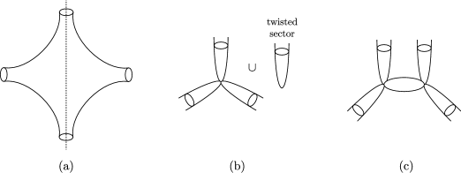
Figure 1. Mirrors of the four-punctured sphere

One can find a similar feature in its toric Calabi-Yau mirror. Through pair-of-pants decomposition, one obtains a mirror LG model $\tilde{W}$ on $O_{\mathbb{P}^{1}}\oplus O_{\mathbb{P}^{1}}(-2)$ which is a resolution of the quotient $\mathbb{C}^{3}/\hat{G}$. The critical loci of $W$ are its codimesion 2 toric strata as depicted in Figure 1 (c). The only difference from the previous picture of the orbifold mirror is $\mathbb{P}^{1}$ component in $crit(\tilde{W})$, which does not actually affect as this $\mathbb{P}^{1}$ component can only support constant (holomorphic) functions.

Torus with three punctures

We next look at the example of a tri-punctured elliptic curve $X$ (Figure 2 (a)), which can be explicitly written as a hypersurface of $(\mathbb{C}^{\ast})^{2}$ defined by $z_{1}+z_{2}+\frac{1}{z_{1}z_{2}}=1$. It admits an action of $G=\mathbb{Z}/3$ by multiplying the third of unity diagonally to $z_{1}$ and $z_{2}$, and the quotient is again the pair-of-pants $P$. $X$ is also well-known as a generic fiber of the mirror $\mathbb{P}^{2}$, and all the three vanishing cycles project to the Seidel Lagrangian $\mathbb{L}$ in $P$. (See [AKO06] or [CHL17] for more details.)

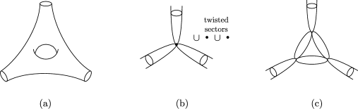
Figure 2. Mirrors of the tri-punctured torus

Through our equivariant construction, its orbifold LG mirror is $[\mathbb{C}^{3}/\hat{G}]$ where the action is generated by $\chi\cdot(x,y,z)=(e^{2\pi i/3}x,e^{2\pi i/3}y,e^{2\pi i/3}z)$. The twisted sectors of $crit(W)/\hat{G}$ in this case does not have additional leg which is consistent with the fact that $X$ only has three cylindrical ends. Instead it contains in addition to $crit(W)$ (the untwisted sector) two isolated points supported over $(0,0,0)$ as twisted sectors associated with $\chi$ and $\chi^{2}$ in $\hat{G}$ (both of which fix $(0,0,0)$).

On the other hand, the gluing construction produces the LG model on $K_{\mathbb{P}^{2}}$ as a mirror, whose associated critical loci is given as in (c) of Figure 2. Observe that it has (degenerate) elliptic curve as a part of the codimension 2 toric strata as well as three legs each isomorphic to $\mathbb{C}$. We believe that degree $1$ cocycles of this elliptic curve defined in a suitable sense (presumably in some mixed hodge structures) should correspond to the two isolated points in the twisted sector in the orbifold mirror.

Extension of the construction in this paper to the case of a nonabelian symmetry $G$ on $X$ primarily requires a replacement of the equivariant Floer complex $CF_{\hat{G}}(\mathbb{L},\mathbb{L})$. Indeed, one can identify this complex with the Floer complex of the union of Lagrangian branes supported over the same Lagrangian $\mathbb{L}$ with various local systems (flat line bundles) coming from characters $\chi\in\hat{G}$. More precisely, a character $\chi$ determines a flat line bundle over $\mathbb{L}$ which is nothing but the diagonal quotient of $\tilde{\mathbb{L}}\times\mathbb{C}$. Here, $\tilde{\mathbb{L}}$ is a chosen lifting of $\mathbb{L}$ in $X$. By definition, the corresponding parallel transport jumps precisely by $\chi(g)$ at the self intersection point $x$ of $\mathbb{L}$ if $x$ is the image of both $\tilde{x}$ and $g\cdot\tilde{x}$ for some $\tilde{x}\in\tilde{\mathbb{L}}$. Along this line, it seems unavoidable to include higher rank local systems associated irreducible representations of $G$ when it is nonabelian. We expect that these lead to a new type of the orbifolded mirror LG model of $X$ when correctly performed, and leave for a future investigation.

Acknowledgement

We would like to thank Cheol-Hyun Cho, Dahye Cho, Jungsoo Kang, Myeonggi Kwon, Jae Hee Lee, Kyoung-Seog Lee, Weiwei Wu for their valuable comments. The work of the first named author is partially funded by the Korea government (MSIT) (No. 2020R1C1C1A01008261 and 2020R1A5A1016126). The work of the third named author is supported by the Korea government(MSIT)(No. 202117221032) and Basic Science Research Program funded by the Ministry of Education (2021R1A6A1A10044154).

2. Preliminaries

In this section, we briefly review basic materials in symplectic cohomology and Lagrangian Floer theory relevant to our construction below, mainly to fix notations and clarify our geometric setup. We will follow [Abo15, RS17] for the former, and [FOOO09] for the latter.

Let $X$ be a Liouville manifold with an exact symplectic form $\omega=d\lambda$. Then $X$ can be decomposed into a compact domain $X^{in}$ with contact boundary $(Y=\partial X^{in},\lambda|_{Y})$ and its complement $X\setminus X^{in}$ symplectomorphic to the symplectization

$$(Y\times[1,+\infty),\>d(R\,\lambda|_{Y})).$$ (2.1)

where $R$ is the coordinate on $[1,+\infty)$ and $\lambda|_{Y}$ serves as a contact form on $Y$. A component of $X\setminus X^{in}$ is called a cylindrical end. In particular, when $X$ is of dimension $2$, each cylindrical end in $X$ is simply

$$C_{1}=(S^{1}\times[1,+\infty),\>dR\wedge d\theta)$$

up to symplectomorphism.

2.1. Symplectic cohomology

Choose a generic Hamiltonian $H:X\to\mathbb{R}$ such that $H|_{X^{in}}:X^{in}\to\mathbb{R}$ is a $C^{2}$-small Morse-Smale function. We assume that the slope of $H$ is linear in $R$ when $R$ is large enough with a small slope that the only 1-periodic orbits are critical points of $H|_{X^{in}}$. We then consider the family $\{wH\}_{w\in\mathbb{Z}_{>0}}$ of Hamiltonians and their associated Hamiltonian Floer cohomologies. In what follows, the same notation $wH$ will denote (by abuse of notation) its perturbation by a small time-dependent function supported near its 1-periodic orbits in order to break $S^{1}$-symmetry. We obtain exactly two nondegenerate orbits from each $S^{1}$-family of 1-periodic orbit of (original) $wH=wH(R)$ after the perturbation. See [CFHW96, Lemma 2.1] for more details.

As usual, the Floer complex $CF(wH)$ is generated by 1-periodic Hamiltonian orbits over the coefficient field $\Bbbk$ (taken to be $\mathbb{C}$ in our application), and we write $\mathfrak{d}$ for its differential that counts pseudo-holomorphic cylinders asymptotic to two orbits (of degree difference 1) at $\pm\infty$. Now the symplectic cochain complex is defined as

$$SC^{\ast}(X):=\bigoplus_{w=1}^{\infty}CF(wH)[\mathbb{q}]$$

equipped with the differential $\mu_{1}:SC^{\ast}(X)\to SC^{\ast+1}(X)$ given by

$$\mu_{1}(x+\mathbb{q}y)=(-1)^{|x|}\mathfrak{d}x+(-1)^{|y|}(\mathbb{q}\mathfrak{d}y+\mathfrak{K}y-y).$$

where $\mathbb{q}$ is a formal variable of degree $-1$ such that $\mathbb{q}^{2}=0$. Here $\mathfrak{K}:CF(wH)\to CF((w+1)H)$ denotes the Floer continuation maps $\mathfrak{K}:CF(wH)\to CF((w+1)H)$ (which is not an isomorphism in this case). One can alternatively define $SC^{\ast}(X)$ as a direct limit

$$SC^{\ast}(X):=\lim_{w\to\infty}CF^{\ast}(wH)$$

of the family $\{CF(wH)\}_{w\geq 1}$ over under this continuation map.

We can make $SC^{\ast}(X)$ into an $A_{\infty}$-algebra extending $\mu_{1}$, for e.g., by letting $\mu_{k}$ counts pseudo-holomorphic maps from cylinders with additional punctures. To construct a moduli of such maps, one needs to specify extra information about these punctures including their locations and asymptotic markers (so as to canonically determine the parametrizations of cylindrical ends near punctures) which is to be partially discussed in the proof of Lemma 2.1 below. In fact, we will assign to each pseudo-holomorphic map for $\mu_{k}$ the following extra datum indicating a special alignment of the punctures.

Lemma 2.1.

One can align punctures and asymptotic markers in the domain of each pseudo-holomorphic map for $\mu_{k}$ along a coherent path with one end corresponding to the output marked point (negative end/puncture).

The alignment of punctures we choose in the proof already appeared in [RS17, 4.6], and is by no chance unique.

Proof.

For $\mu_{1}$, one can simply use the cylinder $S^{1}\times\mathbb{R}$ with coordinates $(t,s)\in S^{1}\times\mathbb{R}$ as our fixed domain. The two ends (punctures) are located at $s=\pm\infty$, and one may choose the $t=0$ line in this case. The domain can be equivalently viewed as $\mathbb{C}P^{1}$, and for $\mu_{2}$, we locate one negative puncture at $z_{0}=0$ and two positive ones at $z_{1}=\infty$, $z_{2}=1$. In particular, this fixes the parametrization of the domain. We then choose the arc $(0,\infty)\subset\mathbb{R}P^{1}$ inside $\mathbb{C}P^{1}$ that passes through all punctures, and let asymptotic markers at punctures parallel with the equator. Therefore a part of the path breaks into the $t=0$ line in the bubbled-off cylinder when $\mathbb{C}P^{1}$ limits to a degenerate configuration which guarantees the Leibnitz rule between $\mu_{1}$ and $\mu_{2}$.

Similarly, we can consider $\mathbb{C}P^{1}$ with four punctures lining up along the equator $\mathbb{R}P^{1}$, and let two adjacent punctures collide along the equator to see that the associativity of $\mu_{2}$ is not affected by our particular choice of a path. One can proceed similarly for maps contributing to higher $\mu_{k}$’s by fixing their domain parametrization to be $\mathbb{C}P^{1}$ and locating the punctures along $\mathbb{R}P^{1}$. ∎

A direct consequence of the lemma is that the domain of each pseudo-holomorphic maps has a canonical path from each input marking (positive puncture) to the output (negative puncture). More precisely, the path follows the $t=0$ line of the cylindrical (positive) end corresponding to $k$-th marked point, runs along the equator of the fixed domain $\mathbb{C}P^{1}$, and merges into the $t=0$ line in the cylindrical (negative) end for the $0$-th marked point. We make the path avoid positive punctures $z_{k+1},z_{k+2},\cdots,$ in the middle by letting it go slightly ‘above’ these punctures (this makes sense as we fixed the domain $\mathbb{C}P^{1}$) until it reaches $z_{0}$. Its image under $u$ is a path in $X$ that joins starting points of the Hamiltonian orbit incident to the $k$-th marked point and that of the output orbit. We denote this path by $\gamma_{u,k}$. Note that the homotopy type of the paths $\gamma_{u,k}$ is preserved under the degeneration of pseudo-holomorphic maps that is responsible for the algebraic structures on $SC^{\ast}(X)$, due to Lemma 2.1. In the equivariant setting below, this data will be used to twist the structures in the existence of the group action.

2.2. Symplectic cohomology of pair-of-pants

We give an explicit description of $SH^{\ast}(P)$ when $P$ is a tri-puntured sphere, as known as the pair-of-pants. It can be neatly represented in terms of $H^{\ast}_{log}(M,D)$ due to the work of [GP20], where we think $M=\mathbb{C}P^{1}$ as a compactification of $P$ with $D=M\setminus P$ consisting of three distinct points, say $q_{\alpha}$, $q_{\beta}$ and $q_{\gamma}$. The description is particularly simple in this case since $D$ is a set of points.

Following [GP20, 3.2], $H^{\ast}_{log}(M,D)$ is generated by $H^{\ast}(P)$ and the cohomology of three circles appearing as the boundary of the real blowup of $M$ along $D$. In our case, these circles can also be identified with boundary circles of small disk neighborhoods of $q_{\alpha}$, $q_{\beta}$ and $q_{\gamma}$. We denote these circles by $S_{\alpha}$, $S_{\alpha}$, $S_{\alpha}$ respectively, and choose (perfect) Morse functions $h_{\alpha},h_{\beta}$ and $h_{\gamma}$ on them. Then the chain-level $H^{\ast}_{log}(M,D)$ is defined by

$$CM^{\ast}(h;P)\oplus t_{\alpha}CM(h_{\alpha};S_{\alpha})[t_{\alpha}]\oplus t_{\beta}CM(h_{\beta};S_{\beta})[t_{\beta}]\oplus t_{\gamma}CM^{\ast}(h_{\gamma};S_{\gamma})[t_{\gamma}]$$ (2.2)

where $h=H$ (regraded as a generic Morse function on $P$), and $t_{\alpha},t_{\beta},t_{\gamma}$ are formal variables of degree $1$. Since we are using perfect Morse functions, the differential on (2.2) automatically vanishes. Moreover, $CM(h_{\alpha};S_{\alpha})$ is generated by two critical points $e_{\alpha}$ and $f_{\alpha}$ with $|e_{\alpha}|=0$ and $|f_{\alpha}|=1$, and similar for $\beta$ and $\gamma$. We set $e,f_{1},f_{2}$ for critical points of $h=H$ as shown in Figure 3. Recall that the actual Hamiltonian we use to define $SH(P)$ is its time-dependent perturbation.

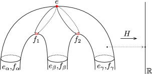
Figure 3. Choice of the Hamiltonian $H$ on $P$ and its critical points in $P^{in}$

The product structure is given in the form of

$$t^{v}x\cdot t^{w}y=t^{v+w}x\star y$$

where $x\star y$ between two critical points of one of $h_{i}$’s counts usual $Y$-shape flow lines composed with the restriction map $CM^{\ast}(h;P)\to CM(h_{\alpha};S_{\alpha})$ (and similarly for $\beta$ and $\gamma$) cf. Figure 4 in [GP20]. In our case, one can deduce all the products from

$$\begin{array}[]{c}f_{1}\star e_{\alpha}=f_{\alpha},\quad e_{\alpha}\star e_{\alpha}=e_{\alpha},\quad e_{\alpha}\star f_{\alpha}=f_{\alpha}\\ f_{1}\star e_{\beta}=-f_{2}\star e_{\beta}=f_{\beta},\quad e_{\beta}\star e_{\beta}=e_{\beta},\quad e_{\beta}\star f_{\beta}=f_{\beta}\\ f_{2}\star e_{\gamma}=f_{\gamma},\quad e_{\gamma}\star e_{\gamma}=e_{\gamma},\quad e_{\gamma}\star f_{\gamma}=f_{\gamma}\end{array}$$ (2.3)

together with the fact that $e$ is the unit. (Note that $e_{\alpha}$ and $f_{\alpha}$ themselves do not belong to the cochain complex.)

By [GP20, Theorem 1.4, Example 1.1], the (low-energy) PSS map gives a ring isomorphism, which do not involve any complicated counting in our case. Under the PSS map, one can identify $e_{\alpha}t_{\alpha}^{i}$ and $f_{\alpha}t_{\alpha}^{i}$ with the two nondegenerate orbits near $q_{\alpha}$ with winding number exactly $i$, and similar for $\beta$ and $\gamma$. From now on, we will not strictly distinguish an element of (2.2) and its corresponding Hamiltonian orbit in $SC^{\ast}(P)$ unless there is a danger of confusion.

$SC^{\ast}(P)$ is graded once we choose a volume form on $P$ and trivialize $T^{\mathbb{C}}P$ accordingly. In our case, we will find it more convenient to use the section of $\Omega_{P}^{\otimes 3}$ to keep the symmetry. Namely, we choose a cubic volume form $\Omega$ (locally $\Omega=\varphi(z)dz^{3}$) on $S^{2}$ which has a double pole at each of points in $D=\{q_{\alpha},q_{\beta},q_{\gamma}\}$. For e.g., one may take $\frac{dz}{z^{2}(z-1)^{2}}$ for $q_{\alpha}=0,q_{\beta}=1,q_{\gamma}=\infty$. This results in the fraction grading on $SC^{\ast}(P)$ for which

$$|t_{\alpha}|=|t_{\beta}|=|t_{\gamma}|=\frac{2}{3},\quad|e_{\alpha}|=|e_{\beta}|=|e_{\gamma}|=0,\quad|f_{\alpha}|=|f_{\beta}|=|f_{\gamma}|=1.$$

The component $CM^{\ast}(h;P)$ carries the usual $\mathbb{Z}$-grading, i.e., $|e|=0,|f_{1}|=|f_{2}|=1$. (The $A_{\infty}$-operation $\mu_{k}$ is of degree $2-k$ with respect to this grading.) See, for e.g., [Ton19, 2.2]. We will use an analogous fractional grading for Lagrangian Floer theory on $P$. Multiplying $3$ to this fraction degrees recovers the usual $\mathbb{Z}/2$-grading on $SC^{\ast}(P)$.

2.3. Orbifold Landau-Ginzburg B-models

Our mirror LG-model $W:\Bbbk^{n}\to\Bbbk$ will carry an action of a finite abelian group $H$. We introduce the construction of the closed-string $B$-model invariant attached to the associated orbifold setting.

Let $\theta_{i}$ and $\partial_{\theta_{i}}$ (for $i=1,\cdots,n$) be variables with $|\theta_{i}|=-1$, $|\partial_{\theta_{i}}|=1$ and

$$\theta_{i}\theta_{j}=-\theta_{j}\theta_{i},\;\;\partial_{\theta_{i}}\partial_{\theta_{j}}=-\partial_{\theta_{j}}\partial_{\theta_{i}},\;\;\partial_{\theta_{i}}\theta_{j}=-\theta_{j}\partial_{\theta_{i}}+\delta_{ij}$$ (2.4)

We recall an elementary definition in terms of above variables.

Definition 2.2.

Let $R$ be a commutative ring. For a sequence $(r_{1},\cdots,r_{n})\subset R$,

$$K^{\ast}(r_{1},\cdots,r_{n}):=(R\langle\theta_{1},\cdots,\theta_{n}\rangle,\sum_{i}r_{i}\partial_{\theta_{i}})$$

is called the Koszul complex of $(r_{1},\cdots,r_{n})$. When $(r_{1},\cdots,r_{n})$ is given as the Jacobian ideal of some $W$, then we will write the corresponding Koszul complex as $(K^{\ast}(\partial W),d_{W})$.

The cochain complex $K^{\ast}(r_{1},\cdots,r_{n})$ is explicitly

Let us denote $K^{-m}(r_{1},\cdots,r_{n})=\bigoplus\limits_{i_{1}<\cdots<i_{m}}R\cdot\theta_{i_{1}}\cdots\theta_{i_{m}}$.

The following notion is an important categorical invariant of singularities.

Definition 2.3.

Let $R$ be a commutative ring. A matrix factorization of $W\in R$ is a $\mathbb{Z}/2$-graded projective $R$-module $P=P_{0}\oplus P_{1}$ together with a morphism $d=(d_{0},d_{1})$ of degree 1 such that

$$d^{2}=W\cdot{\rm id}.$$

Let $\phi:(P,d)\to(Q,d^{\prime})$ be a morphism of degree $j\in\mathbb{Z}/2$. Define

$$D\phi:=d^{\prime}\circ\phi-(-1)^{|\phi|}\phi\circ d$$

and define the composition of morphisms in the usual sense. This defines a dg-category of matrix factorizations $(MF(W),D,\circ)$.

Definition 2.4.

Let $W\in R$ and let $H$ be a group which acts on $R$ leaving $W$ invariant. An $H$-equivariant matrix factorization of $W$ is a matrix factorization $(P,d)$ where $P$ is equipped with an $H$-action, and $d$ is $H$-equivariant. An $H$-equivariant morphism $\phi$ between two $H$-equivariant matrix factorizations $(P,d)$ and $(Q,d^{\prime})$ is an $H$-equivariant morphism of $\mathbb{Z}/2$-graded $R$-modules $P$ and $Q$. Again, $H$-equivariant matrix factorizations form a dg-category $(MF_{H}(W),D,\circ)$.

From now on we will consider $W\in R=\Bbbk[x_{1},\cdots,x_{n}]$ and $H$ is a finite abelian group acting on $R$ leaving $W$ invariant. We call the pair $(W,H)$ an orbifold LG B-model. Furthermore we will assume that $H$ acts on $R$ diagonally, which means that for $h\in H$,

$$h\cdot x_{i}=h_{i}x_{i}$$ (2.5)

for some $h_{i}\in\Bbbk^{*}$. We introduce the following notation:

$$x_{i}^{h}:=\begin{cases}x_{i}&{\textrm{ if }}h\cdot x_{i}=x_{i},\\ 0&{\textrm{ if }}h\cdot x_{i}\neq x_{i}.\end{cases}$$

Let $S=\Bbbk[x_{1},\cdots,x_{n},x_{1}^{\prime},\cdots,x_{n}^{\prime}]$. Given an orbifold LG model $(W,H)$.

$$\nabla_{i}W:=\frac{W(x_{1}^{\prime},\cdots,x_{i}^{\prime},x_{i+1},\cdots,x_{n})-W(x_{1}^{\prime},\cdots,x_{i-1}^{\prime},x_{i},\cdots,x_{n})}{x_{i}^{\prime}-x_{i}}\in S$$

and define an $(H\times H)$-equivariant matrix factorization of $W\boxminus W:=W(x_{1}^{\prime},\cdots,x_{n}^{\prime})-W(x_{1},\cdots,x_{n})$ by

$$\Delta_{W}^{H\times H}:=\bigoplus_{h\in H}\Big{(}S\langle\theta_{1},\cdots,\theta_{n}\rangle,\sum_{i=1}^{n}\big{(}(x_{i}^{\prime}-h\cdot x_{i})\theta_{i}+\nabla_{i}W\cdot\partial_{\theta_{i}}|_{h\cdot x\to x}\big{)}\Big{)},$$

with $H$-action on variables $\{\theta_{1},\cdots,\theta_{n},\partial_{\theta_{1}},\cdots,\partial_{\theta_{n}}\}$ defined by

$$h\cdot\theta_{i}:=h_{i}^{-1}\theta_{i},\;\;h\cdot\partial_{\theta_{i}}:=h_{i}\partial_{\theta_{i}}$$

when $h\cdot x_{i}=h_{i}x_{i}$. Also, for any $S$ (or $R$)-linear map $F$, $F|_{h\cdot x\to x}$ means that we replace all variables $\{x_{1},\cdots,x_{n}\}$ in $F$ by $\{h\cdot x_{1},\cdots,h\cdot x_{n}\}$ accordingly.

Denote each $h$-summand of $\Delta_{W}^{H\times H}$ by $\Delta_{W}^{h}$. We recall the following.

Lemma 2.5 ([CL20]).

We have a quasi-isomorphism

$$hom_{MF_{H\times H}(W\boxminus W)}(\Delta_{W}^{H\times H},\Delta_{W}^{H\times H})\cong\big{(}\bigoplus_{h\in H}hom_{MF(W\boxminus W)}(\Delta_{W}^{1},\Delta_{W}^{h})\big{)}^{H}.$$

Let us define following (ordered) subsets of $\{1,\cdots,n\}$:

$$I_{h}:=\{i\mid hx_{i}\neq x_{i}\},\quad I^{h}:=I_{h}^{c}.$$

Recall that if $W$ has only isolated singularity, then $\mathrm{Hom}_{MF_{H\times H}(W\boxminus W)}(\Delta_{W}^{H\times H},\Delta_{W}^{H\times H})$ is isomorphic to the orbifold Jacobian algebra $\mathrm{Jac}(W,H)$ which is given by following:

$$\mathrm{Jac}(W,H)=\big{(}\bigoplus_{h\in H}\mathrm{Jac}(W^{h})\cdot\xi_{h}\big{)}^{H}$$

where

• $W^{h}=W(x_{1}^{h},\cdots,x_{n}^{h})\in k[x_{1}^{h},\cdots,x_{n}^{h}]$,

• $\mathrm{Jac}(W^{h})=k[x_{1}^{h},\cdots,x_{n}^{h}]/\partial W^{h}$ where $\partial W^{h}:=(\partial_{x_{i}}W^{h}:i\in I^{h})$ is the Jacobian ideal of $W^{h}$,

• $\xi_{h}$ is a formal generator of degree $d_{h}:=|I_{h}|$.

For general $W$ which may have nonisolated singular locus, we still have the following result.

Proposition 2.6.

We have a module isomorphism

$$\mathrm{Hom}_{MF_{H\times H}(W\boxminus W)}(\Delta_{W}^{H\times H},\Delta_{W}^{H\times H})\cong\big{(}\bigoplus_{h\in H}H^{\ast}\big{(}K^{\ast}(\partial W^{h})\big{)}\cdot\theta_{I_{h}}\big{)}^{H}.$$ (2.6)

Proof.

The matrix factorization $\Delta_{W}^{h}$ is constructed by the resolution of a shifted MCM module $S/(x_{1}^{\prime}-h\cdot x_{1},\cdots,x_{n}^{\prime}-h\cdot x_{n})[-n]$ over the hypersurface ring $S/(W\boxminus W)$. Hence we have

$$hom_{MF(W\boxminus W)}(\Delta_{W}^{1},\Delta_{W}^{h}) \simeq hom_{S}\big{(}\Delta_{W}^{1},S/(x_{1}^{\prime}-h\cdot x_{1},\cdots,x_{n}^{\prime}-h\cdot x_{n})[-n]\big{)}$$

$$\simeq hom_{S}\big{(}\Delta_{W}^{1}[n],S/(x_{1}^{\prime}-h\cdot x_{1},\cdots,x_{n}^{\prime}-h\cdot x_{n})\big{)}$$

$$\simeq(\Delta_{W}^{1})^{\vee}[-n]\otimes_{S}\big{(}S/(x_{1}^{\prime}-h\cdot x_{1},\cdots,x_{n}^{\prime}-h\cdot x_{n})\big{)}.$$ (2.7)

By self-duality of Koszul matrix factorizations, $(\Delta_{W}^{1})^{\vee}[-n]$ is quasi-isomorphic to $\Delta_{W}^{1}$. Hence we have

$$\eqref{homcomplex}\simeq\big{(}R\langle\theta_{1},\cdots,\theta_{n}\rangle,d|_{h\cdot x\to x^{\prime}}\big{)}.$$

The latter is the following $\mathbb{Z}/2$-graded double complex:

with

$$d_{hor}:=\sum_{i=1}^{n}(h\cdot x_{i}-x_{i})\theta_{i},\quad d_{vert}:=\sum_{i=1}^{n}\nabla_{i}W\cdot\partial_{\theta_{i}}|_{h\cdot x\to x^{\prime}}.$$

We compute its cohomology by spectral sequence from vertical filtration. The first page is the cohomology with respect to $d_{hor}$. The $i$th row is

and it is quasi-isomorphic to the following complex:

where $R^{h}:=R/(x_{i}:i\in I_{h})$. Therefore, the induced differential $d_{1}$ on $E_{1}$ is given by

$$\sum_{i\in I^{h}}\nabla_{i}W(x,h\cdot x)\partial_{\theta_{i}}=\sum_{i\in I^{h}}(\partial_{i}W^{h})\partial_{\theta_{i}},$$

hence each column is isomorphic to the (degree-)shifted Koszul complex of the Jacobian ideal $\partial W^{h}$. Here the column is referred to be shifted in the sense that $\theta_{I_{h}}$ is multiplied to the original complex.

It remains to show that $d_{i}=0$ on $E_{i}$ for all $i\geq 2$. Let $\displaystyle\sum_{J:I_{h}\subset J}f_{J}\theta_{J}$ be a cocycle of $(E_{1},d_{1})$. Then we have

$$\sum_{\stackrel{{\scriptstyle J:I_{h}\subset J}}{{i\in J}}}\nabla_{i}W(x,h\cdot x)f_{J}\frac{\partial\theta_{J}}{\partial\theta_{i}}=\sum_{j\in I_{h}}(h\cdot x_{j}-x_{j})\theta_{j}\big{(}\sum_{K}g_{K}\theta_{K}\big{)}$$

for some $\sum_{K}g_{K}\theta_{K}$, so

$$d_{2}(\sum f_{J}\theta_{J})=\sum_{i}\sum_{K}\nabla_{i}W(x,h\cdot x)g_{K}\frac{\partial\theta_{K}}{\partial\theta_{i}}.$$

But each summand $g_{K}\theta_{K}$ is given by $K=J^{\prime}-{j}$ for some $J^{\prime}$ and $j\in I_{h}$, so $d_{2}=0$ on $E_{2}$. It implies that $d_{\geq 2}=0$. ∎

Definition 2.7.

Given an orbifold LG model $(W,H)$,

$$Kos(W,H):=\big{(}\bigoplus_{h\in H}H^{\ast}\big{(}K^{\ast}(\partial W^{h})\big{)}\cdot\theta_{I_{h}}\big{)}^{H}$$

is called its orbifold Koszul algebra whose product structure is given by the isomorphism (2.6). (When $H=1$, we simply write $Kos(W)$ which agrees with the cohomology of $(K^{\ast}(\partial W),d_{W})$.)

2.4. Finite group action on Lagrangian Floer theory and semidirect product

We briefly recall the construction of semidirect product $A_{\infty}$-algebras following [CL20]. Its (weak) Maurer-Cartan deformation gives rise to the mirror orbifold LG model to which we will apply the construction in 2.3.

Consider a symplectic manifold $X$ on which a finite abelian group $G$ acts. In cases in which we are interested, we always have a (possibly immersed) Lagrangian submanifold $\mathbb{L}\subset X/G$ with the following properties: there is an embedded Lagrangian lift $\mathbb{L}_{1}\subset X$ of $\mathbb{L}$, and if we let $\mathbb{L}_{g}:=g\cdot\mathbb{L}_{1}$ for $g\in G$, we have $\mathbb{L}_{g_{1}}\neq\mathbb{L}_{g_{2}}$ whenever $g_{1}\neq g_{2}$.

After fixing the lift $\mathbb{L}_{1}$, we have a natural identification of Floer complexes:

$$CF(\mathbb{L},\mathbb{L})\cong\bigoplus_{g\in G}CF(\mathbb{L}_{1},\mathbb{L}_{g}).$$

From now on we will freely use this identification for $CF(\mathbb{L},\mathbb{L})$.

Let ${\widehat{G}}=\mathrm{Hom}(G,U(1))$ be the character group of $G$. Following [CHL21, Chapter 7], we have a natural ${\widehat{G}}$-action $\rho$ on $CF(\mathbb{L},\mathbb{L})$ as follows: for $v_{g}\in CF(\mathbb{L}_{1},\mathbb{L}_{g})$ and $\chi\in{\widehat{G}}$,

$$\rho(\chi)(v_{g}):=\chi(g^{-1})v_{g}.$$

We recall the notion of semi-direct products.

Definition 2.8 ([Sei11]).

Given an $A_{\infty}$-algebra $\mathcal{A}$ and $H$-action $\rho$ on $\mathcal{A}$, the semi-direct product $A_{\infty}$-algebra structure on $\mathcal{A}\otimes\Bbbk[H]$ is defined as

$$\begin{split}&m_{k}(w_{1}\otimes\chi_{1},\cdots,w_{k}\otimes\chi_{k})\\ :=&m_{k}\big{(}\rho(\chi_{2}\cdots\chi_{k})(w_{1}),\rho(\chi_{3}\cdots\chi_{k})(w_{2}),\cdots,\rho(\chi_{k})(w_{k-1}),w_{k}\big{)}\otimes\chi_{1}\cdots\chi_{k}.\end{split}$$ (2.8)

Remark 2.9.

Observe that for $v_{g_{1}}\in CF(\mathbb{L}_{1},\mathbb{L}_{g_{1}}),\cdots,v_{g_{k}}\in CF(\mathbb{L}_{1},\mathbb{L}_{g_{k}})$, we can rewrite $m_{k}$ on $CF(\mathbb{L},\mathbb{L})\otimes\Bbbk[{\widehat{G}}]$ by

$$\begin{split}&m_{k}(v_{g_{1}}\otimes\chi_{1},\cdots,v_{g_{k}}\otimes\chi_{k})\\ =&m_{k}\big{(}v_{g_{1}},\chi_{2}(g_{1}^{-1})v_{g_{2}},\cdots,\chi_{k}(g_{1}^{-1}\cdots g_{k-1}^{-1})v_{g_{k}}\big{)}\otimes\chi_{1}\cdots\chi_{k}.\end{split}$$

This formulation is useful for the interpretation of semi-direct product $A_{\infty}$-structure in terms of “path-decorated” discs which will appear later.

For notational simplicity, we write by

$$CF(\mathbb{L},\mathbb{L};\hat{G}):=CF(\mathbb{L},\mathbb{L})\otimes\Bbbk[{\widehat{G}}]$$ (2.9)

the corresponding module with the $A_{\infty}$-structure in Definition 2.8 from now on.

Lemma 2.10 ([Sei11, CL20]).

For $\widetilde{\mathbb{L}}:=\bigoplus_{g\in G}\mathbb{L}_{g}\subset X$, we have an $A_{\infty}$-isomorphism

$$\Phi:CF(\mathbb{L},\mathbb{L};\hat{G})\to CF(\widetilde{\mathbb{L}},\widetilde{\mathbb{L}})$$

where $\Phi_{1}(v\otimes\chi)=\sum_{g\in G}\chi(g^{-1})(g\cdot v)$ and $\Phi_{\geq 2}=0$.

Next, we consider the deformation of $\mathbb{L}$ by weak bounding cochains. Recall that $b\in CF^{1}(\mathbb{L},\mathbb{L})$ is called a (weak) bounding cochain if it satisfies

$$m_{0}+m_{1}(b)+m_{2}(b,b)+\cdots=W(b)\cdot e_{\mathbb{L}}.$$

for $W(b)\in\Bbbk$ where $e_{\mathbb{L}}$ is the unit (which can be specified in the Morse model we will use in the later applications). $W$ is called the (Floer) potential. We denote the set of all bounding cochains by $MC_{weak}(\mathbb{L})$. Throughout, we work with an assumption that there exist elements $X_{1},\cdots,X_{n}\in CF^{1}(\mathbb{L},\mathbb{L})$ such that any $\Bbbk$-linear combination $b$ of $X_{1},\cdots,X_{n}$ satisfies weak Maurer-Cartan equation. Hence $MC_{weak}(\mathbb{L})$ contains their linear span isomorphic to $\Bbbk^{n}$. Define

$$CF((\mathbb{L},b),(\mathbb{L},b)):=CF(\mathbb{L},\mathbb{L})\otimes_{\Bbbk}R,$$ (2.10)

i.e., we extend the coordinate to obtain an $A_{\infty}$-algebra over $R=\Bbbk[x_{1},\cdots,x_{n}]$. This comes with some technical subtlety which will be addressed shortly. One can check that $b=x_{1}X_{1}+\cdots+x_{n}X_{n}$ is a weak bounding cochain on $CF((\mathbb{L},b),(\mathbb{L},b))$ where $A_{\infty}$-operations $m_{k}^{b,\cdots,b}$ on $CF((\mathbb{L},b),(\mathbb{L},b))$ are $b$-deformed $m_{k}$ on $CF(\mathbb{L},\mathbb{L})$ with coefficients of $b$ taken from $R$.

In full generality, $R$ should be the quotient of $\Lambda\{x_{1},\cdots,x_{n}\}$ by $f_{j}$’s appearing as coefficients of nonunit generators in $CF(\mathbb{L},\mathbb{L})$ in the (multi-)linear expansion of

$$m_{0}+m_{1}(b)+m_{2}(b,b)+\cdots=\tilde{W}(b)\cdot e_{\mathbb{L}}+\sum_{j}f_{j}(x_{1},\cdots,x_{n})Y_{j}$$

using the rule $m_{k}(x_{i_{1}}X_{i_{1}},\cdots,x_{i_{k}}X_{i_{k}})=x_{i_{k}}\cdots x_{i_{1}}$. Here $\Lambda\{x_{1},\cdots,x_{n}\}$ consists of noncommutative power series in $x_{i}$’s with valuations of coefficients bounded below. Notice that variables a priori do not commute. However, for our purpose, it suffices to work with a polynomial ring over $\mathbb{C}$ since (i) there is no convergence issues due to some strong finiteness conditions (see Lemma 2.14) and (ii) $f_{j}$’s are given as commutators. Therefore any $\mathbb{C}$-linear combination of $X_{i}$’s serves as a weak bounding cochian in our main application.

Remark 2.11.

There is an obvious structural similarity between $CF_{R}(\mathbb{L},\mathbb{L})$ and (a certain component of) the Hochschild cochain complex $CH^{\ast}(CF(\mathbb{L},\mathbb{L}),CF(\mathbb{L},\mathbb{L}))$. In fact, if one identifies an element $x_{i_{k}}\cdots x_{i_{1}}Y\in CF_{R}(\mathbb{L},\mathbb{L})$ with a map $CF(\mathbb{L},\mathbb{L})^{\otimes k}\to CF(\mathbb{L},\mathbb{L})$ that sends the generator $X_{i_{1}}\otimes\cdots\otimes X_{i_{k}}$ to $Y$ and all the others to zero, then differentials and products on both sides match (up to a coherent change of signs). The only difference is that $x_{i}$’s do not commute on Hochschild side.

Let us now consider the ${\widehat{G}}$-equivariant twist of the above construction.

Lemma 2.12.

Let $b=x_{1}X_{1}+\cdots+x_{n}X_{n}$ be a weak bounding cochain on $CF((\mathbb{L},b),(\mathbb{L},b))$. Then $b\otimes 1$ is a weak bounding cochain on $CF((\mathbb{L},b),(\mathbb{L},b))\otimes\Bbbk[{\widehat{G}}]$.

Similarly to (2.9), we denote

$$CF((\mathbb{L},b),(\mathbb{L},b);\hat{G}):=CF((\mathbb{L},b),(\mathbb{L},b))\otimes\Bbbk[{\widehat{G}}]$$

in what follows. It is helpful to spell out $m_{k}^{b\otimes 1,\ldots,b\otimes 1}$ operations explicitly.

$$m_{k}^{b\otimes 1,\ldots,b\otimes 1}(a_{1}\otimes\chi_{1},\cdots,a_{k}\otimes\chi_{k})$$ (2.11)

$$= m_{k}^{\rho(\chi_{1}\cdots\chi_{k})b,\rho(\chi_{2}\cdots\chi_{k})b,\cdots,\rho(\chi_{k})b,b}\big{(}\rho(\chi_{2}\cdots\chi_{k})a_{1},\rho(\chi_{3}\cdots\chi_{k})a_{2},\cdots,a_{k}\big{)}\otimes\chi_{1}\cdots\chi_{k},$$

where $\rho(\chi)b=\sum_{i}x_{i}\cdot\rho(\chi)(X_{i}).$

Recall that we employed ${\widehat{G}}$-action $\rho$ on $CF(\mathbb{L},\mathbb{L})$ to define $CF((\mathbb{L},b),(\mathbb{L},b);\hat{G})$. Now, on $CF((\mathbb{L},b),(\mathbb{L},b);\hat{G})$, we consider an extended ${\widehat{G}}$-action as follows:

$$\chi\cdot(r(x)v\otimes\eta):=r(\chi\cdot x)\rho(\chi)v\otimes\eta.$$ (2.12)

Let $S=\Bbbk[x_{1},\cdots,x_{k},x_{1}^{\prime},\cdots,x_{k}^{\prime}]$, $b^{\prime}=x_{1}^{\prime}X_{1}+\cdots+x_{n}^{\prime}X_{n}$, and consider $CF((\mathbb{L},b),(\mathbb{L},b^{\prime}))$ which is defined analogously to (2.10). As a module

$$CF((\mathbb{L},b),(\mathbb{L},b^{\prime}))=CF(\mathbb{L},\mathbb{L})\otimes_{\Bbbk}S$$ (2.13)

and it has a curved differential $m_{1}^{b,b^{\prime}}$ deformed by $b$ and $b^{\prime}$ whose coefficients are taken from $S$. It is a (curved) $A_{\infty}$-bimodule, but we may regard it as a matrix factorization of $W\boxminus W:=W(x_{1}^{\prime},\cdots,x_{n}^{\prime})-W(x_{1},\cdots,x_{n})$.

Proposition 2.13.

• $m_{k}^{b\otimes 1,\ldots,b\otimes 1}$ is equivariant with respect to the ${\widehat{G}}$-action in (2.12) so $m_{k}^{b\otimes 1,\ldots,b\otimes 1}$ defines a well-defined $A_{\infty}$-structure on $(CF((\mathbb{L},b),(\mathbb{L},b);\hat{G}))^{{\widehat{G}}}$.

• If $CF((\mathbb{L},b),(\mathbb{L},b^{\prime}))$ in (2.13) is isomorphic to $\Delta_{W}^{1}$, then $(CF((\mathbb{L},b),(\mathbb{L},b);\hat{G}))^{{\widehat{G}}}$ is $A_{\infty}$-isomorphic to $hom_{MF_{{\widehat{G}}\times{\widehat{G}}}(W\boxminus W)}(\Delta_{W}^{{\widehat{G}}\times{\widehat{G}}},\Delta_{W}^{{\widehat{G}}\times{\widehat{G}}})$, so we also have

  $$H^{\ast}((CF((\mathbb{L},b),(\mathbb{L},b);\hat{G}))^{{\widehat{G}}})\cong Kos(W,{\widehat{G}}).$$

The above results are shown in [CL20] when $W$ has an isolated singularity. Their proofs only involve algebraic formalism, and the same proof works for nonisolated cases as well.

2.5. The Seidel Lagrangian in the pair-of-pants $P$

Let us look at the example of the pair-of-pants $P$ again. We apply the construction in 2.4 to a certain immersed Lagrangian $\mathbb{L}$. We take $\mathbb{L}$ to be the immersed circle with three transversal self-intersection points $X,Y,Z$ depicted in Figure 4, which carries a nontrivial spin structure. The nontrivial spin structure (marked as $\circ$ in Figure 4) can be represented by fixing a generic point on $\mathbb{L}$ so that the sign of a pseudo-holomorphic curve changes each time its boundary passes through the point. This immersed circle was first introduced in [Sei11], and is often called the Seidel Lagrangian for this reason. Sheridan [She11] used $\mathbb{L}$ and its higher dimensional analogues to study homological mirror symmetry of pair-of-pants.

Figure 4. The Seidel Lagrangian $\mathbb{L}$

The Maurer-Cartan formalism on $CF(\mathbb{L},\mathbb{L})$ gives rise to a LG model as follows. Recall that $CF(\mathbb{L},\mathbb{L})$ takes two generators from the cohomology of $S^{1}$ which is the domain of the immersion, and two generators from each self-intersection points of complementary degrees. Denote by $e_{\mathbb{L}}$ and $f_{\mathbb{L}}$ the unit and the point class in $CF(\mathbb{L},\mathbb{L})$ from $H^{\ast}(S^{1})$, and write $X,\bar{X}$, $Y,\bar{Y}$, $Z,\bar{Z}$ for immersed generators supported at the self-intersection points $X$, $Y$, $Z$ respectively with degrees $|X|=|Y|=|Z|\equiv 1,|\bar{X}|=|\bar{Y}|=|\bar{Z}|\equiv 0\mod 2.$ In practice, we prefer a fractional grading induced by the volume form $\Omega$ in parallel to 2.2, which results in

$$|X|=|Y|=|Z|=\frac{1}{3},\quad|\bar{X}|=|\bar{Y}|=|\bar{Z}|=\frac{2}{3},\quad|e_{\mathbb{L}}|=0,\quad|f_{\mathbb{L}}|=1$$

as already computed in [Sei11, Section 10]. We take $1/3$ of the ‘index’ therein as our fractional degree in order to keep the degree of $m_{k}$ to be $2-k$ as usual. (Our $m_{k}$ corresponds to the $0$-th order term $m_{0}^{k}$ [Sei11]).

By the reflection argument, one can show that $b=xX+yY+zZ$ solves the weak Maurer-Cartan equation

$$m_{1}(b)+m_{2}(b,b)+\cdots=W(b)\cdot e_{\mathbb{L}}$$

with $W(b)=W(x,y,z)=xyz$. Technically $x,y,z$ should be taken from the positive valuation part of the coefficient ring to control the convergence. For our purpose, $x,y,z$ can be taken from $\mathbb{C}$ as we will explain in Lemma 2.14. We refer readers to [Sei11] or [CHL17] for details on the $A$-infinity structure on $CF(\mathbb{L},\mathbb{L})$. Indeed, computations here are much simpler than ones in the references which consider the (orbifold-)compactification of $P$.

We justify the usage of coefficients $x,y,z$ over $\mathbb{C}$ in the following lemma.

Lemma 2.14.

For the Seidel Lagrangian $\mathbb{L}$ in the pair-of-pants $P$, the Floer complex $CF((\mathbb{L},b),(\mathbb{L},b))$ regarded as a dga can be defined over $\mathbb{C}$. In particular, $b=xX+yY+zZ$ can be taken over $\mathbb{C}$-coefficients accordingly (i.e., $x,y,z$ can be arbitrary complex numbers).

Proof.

The only issue is the convergence for $m_{1}^{b,b}$ and $m_{2}^{b,b,b}$, as they are given in the form of

$$m_{k}^{b,\cdots,b}(Z_{1},\cdots,Z_{k})=\sum m_{k^{\prime}\geq k}(b,\cdots,b,Z_{1},b,\cdots,b,Z_{k},b,\cdots,b)$$ (2.14)

where we allow to insert arbitrarily many $b$’s. However, in our particular situation, (2.14) is always a finite sum. To see this, one can use aforementioned fractional grading. When $k=1,2$, (2.14) must be a finite sum, since inserting $b$ each time increases the total degree of input by $1/3$ whereas the degree of the operation drops by $1$ for the additional number of inputs. ∎

Formally, one can think of $x,y,z$ as the dual of $X,Y,Z$ where the latter is viewed as the element of the bar construction $B(CF(\mathbb{L},\mathbb{L}))=\oplus_{k}CF(\mathbb{L},\mathbb{L})^{\otimes k}[1]$. Thus their gradings are naturally given as

$$|x|=-(|X|-1)=\frac{2}{3},\quad|y|=\frac{2}{3},\quad|z|=\frac{2}{3}$$

from the fractional grading on $CF(\mathbb{L},\mathbb{L})$. In particular, $W$ has degree $2$.

We now describe the ring structure of the cohomology of the extended Floer complex $CF((\mathbb{L},b),(\mathbb{L},b))$ defined in (2.10). First, the differential acts on generators as

$$m_{1}^{b,b}(X)=yze_{\mathbb{L}},\quad m_{1}^{b,b}(Y)=zxe_{\mathbb{L}},\quad m_{1}^{b,b}(Z)=xye_{\mathbb{L}},$$

$$m_{1}^{b,b}(e_{\mathbb{L}})=0,\quad m_{1}^{b,b}(f_{\mathbb{L}})=xy\bar{Z}+yz\bar{X}+zx\bar{Y}.$$

The most of computations of $m_{1}^{b,b}$ are simply a reinterpretation of [Sei11, Section 10] for our boundary-deformed $A_{\infty}$-operations. One also finds from the same reference that

$$m_{2}^{b,b,b}(X,Y)=\bar{Z}+ze_{\mathbb{L}},\quad m_{2}^{b,b,b}(Y,X)=-\bar{Z}.$$

Taking $m_{1}^{b,b}$ of the first equation leads to

$$m_{1}^{b,b}(\bar{Z})=m_{2}^{b,b,b}(yze_{\mathbb{L}},Y)+m_{2}^{b,b,b}(X,zxe_{\mathbb{L}})=z(xX-yY)$$

by the Leibniz rule. To see this more geometrically, there are actually nontrivial pearl trajectories with $4$ marked points involving two constant pearl components, which are incident to $Z,\bar{Z}$ and $X,\bar{X}$ respectively, and similar for the other. Using the symmetric arguments, we obtain

$$m_{1}^{b,b}(\bar{X})=x(yY-zZ),\quad m_{1}^{b,b}(\bar{Y})=y(zZ-xX),\quad m_{1}^{b,b}(\bar{Z})=z(xX-yY).$$

Therefore generating cocycles of the cohomology as a $\mathbb{C}[x,y,z]$-module are

$$e_{\mathbb{L}},\quad yY-zZ,\quad xX-yY$$ (2.15)

whose module structure is determined by

$$\begin{split}xy\,e_{\mathbb{L}}=yz\,e_{\mathbb{L}}=zx\,e_{\mathbb{L}}=z(&xX-yY)=x(yY-zZ)=0,\\ y(xX-yY)&=-y(yY-zZ)\end{split}$$ (2.16)

where the last relation is obtained from $y(zZ-xX)=0$ modulo coboundaries of $m_{1}^{b,b}$.

Finally, products among these generators which do not involve $e_{\mathbb{L}}$ vanish as the following computation shows.

$$m_{2}^{b,b,b}(yY-zZ,xX-yY) =m_{2}^{b,b,b}(yY,xX-yY)-m_{2}^{b,b,b}(zZ,xX-yY)$$

$$=xy\,m_{2}^{b,b,b}(Y,X)-zx\,m_{2}^{b,b,b}(Z,X)+yz\,m_{2}^{b,b,b}(Z,Y)$$

$$=-xy\bar{Z}-zx\bar{Y}-yz\bar{X}=-m_{1}^{b,b}(f_{\mathbb{L}})=0$$

$$m_{2}^{b,b,b}(xX-yY,xX-yY) =-xy\left(m_{2}^{b,b,b}(X,Y)+m_{2}^{b,b,b}(Y,X)\right)=-xyz\,e_{\mathbb{L}}=0.$$

Here we used the extra fact that $m_{2}^{b,b,b}(X,X)=m_{2}^{b,b,b}(Y,Y)=0$ since its associated moduli is obviously empty.

Now suppose we have an abelian cover $X$ of the pair-of-pants $P$, and denote its deck transformation group by $G$. Applying the construction 2.4, we have an action of the dual group $\hat{G}:=\hom(G,U(1))$ on the Landau-Ginzburg model. More precisely, $\hat{G}$ acts on $\mathbb{C}[x,y,z]$ by

$$\chi\cdot x=\chi(g_{X})x,\quad\chi\cdot y=\chi(g_{Y})y,\quad\chi\cdot z=\chi(g_{Z})z$$

where $g_{X}$ is determined by the condition $\widetilde{X}\in\widetilde{\mathbb{L}}\cap g_{X}\cdot\widetilde{\mathbb{L}}$ for some lifting $\widetilde{\mathbb{L}}$ of $\mathbb{L}$ and similar for $y$ and $z$. The action leaves $W$ invariant.

We next investigate the closed-string B-model invariants of the LG mirror $W(x,y,z)=xyz$ and its orbifoldings with respect to the action of the dual group $\hat{G}$.

2.6. Orbifold Koszul cohomology of $(xyz,{\widehat{G}})$

Let $G$ be a finite abelian group which is the deck transformation group for the covering $X$ of the pair-of-pants $P$. Then ${\widehat{G}}$ acts diagonally on $\mathbb{C}[x,y,z]$ and the polynomial $W=xyz$ is invariant under ${\widehat{G}}$-action. For $h\in{\widehat{G}}$ we have three cases.

1. $h=1$,

2. $h$ acts nontrivially on two variables,

3. $h$ acts nontrivially on three variables.

In case (1), the shifted Koszul complex $K^{\ast}(\partial W^{h})=K^{\ast}(\partial W)$ is given by

The shift is trivial since $I_{h}=\emptyset$ for $h=1$. The resulting cohomology is given as

$$H^{i}(K^{\ast}(\partial W))=\begin{cases}\frac{\langle x\theta_{x}-y\theta_{y},y\theta_{y}-z\theta_{z}\rangle}{\langle yz\theta_{y}-xz\theta_{x},xz\theta_{z}-xy\theta_{y},yz\theta_{z}-xy\theta_{x}\rangle}&i=-1\\ \mathbb{C}[x,y,z]/\langle xy,yz,xz\rangle&i=0\\ 0&{\textrm{otherwise}}\end{cases}$$

(see 4.2 for detailed computations) and $H^{i}(K^{\ast}(\partial W))^{{\widehat{G}}}$ is the set of ${\widehat{G}}$-invariant elements.

In case (2) we have $W^{h}=0$. Assume for example that $z$ is the $h$-invariant variable (we can handle other two cases similarly). Then the shifted Koszul complex $K^{\ast}(\partial W^{h})\cdot\theta_{x}\theta_{y}$ is

and evidently

$$(H^{-1}(K^{\ast}(\partial W^{h}))\cdot\theta_{x}\theta_{y})^{\widehat{G}}\cong(\mathbb{C}[z]\theta_{z}\theta_{x}\theta_{y})^{\widehat{G}},\quad(H^{0}(K^{\ast}(\partial W^{h}))\cdot\theta_{x}\theta_{y})^{\widehat{G}}\cong(\mathbb{C}[z]\theta_{x}\theta_{y})^{\widehat{G}}.$$

For the case (3), we do not have any element of Jacobian ideal because $Fix(h)=\{0\}$, and the shifted Koszul complex is

By the second statement of Proposition 2.13 and the following, we can relate the Floer theory of $\mathbb{L}$ and Koszul cohomology of $(xyz,{\widehat{G}})$.

Proposition 2.15.

There is an isomorphism

$$\eta:CF((\mathbb{L},xX+yY+zZ),(\mathbb{L},x^{\prime}X+y^{\prime}Y+z^{\prime}Z))\cong\Delta_{W}^{1}.$$

Proof.

Let $\{f_{\mathbb{L}},X,Y,Z,e_{\mathbb{L}},\bar{X},\bar{Y},\bar{Z}\}$ be an ordered basis of $CF(\mathbb{L},\mathbb{L})$ as a free module. $m_{1}^{xX+yY+zZ,x^{\prime}X+y^{\prime}Y+z^{\prime}Z}$ can be computed explicitly using the same argument as in 2.5, and in the matrix form with respect to the above basis, it is given as

$$m_{1}^{xX+yY+zZ,x^{\prime}X+y^{\prime}Y+z^{\prime}Z}=\left(\begin{array}[]{cccccccc}0&0&0&0&0&x^{\prime}-x&y^{\prime}-y&z^{\prime}-z\\ 0&0&0&0&x^{\prime}-x&0&-xy&z^{\prime}x\\ 0&0&0&0&y^{\prime}-y&xy&0&-y^{\prime}z^{\prime}\\ 0&0&0&0&z^{\prime}-z&-z^{\prime}x&y^{\prime}z^{\prime}&0\\ 0&y^{\prime}z^{\prime}&z^{\prime}x&xy&0&0&0&0\\ y^{\prime}z^{\prime}&0&z^{\prime}-z&y-y^{\prime}&0&0&0&0\\ z^{\prime}x&z-z^{\prime}&0&x^{\prime}-x&0&0&0&0\\ xy&y^{\prime}-y&x-x^{\prime}&0&0&0&0&0\end{array}\right).$$

Then the isomorphism $\eta$ is given by

$$\begin{array}[]{c}\eta(X)=\theta_{x},\;\eta(Y)=\theta_{y},\;\eta(Z)=\theta_{z},\;\eta(-f_{\mathbb{L}})=\theta_{x}\theta_{y}\theta_{z},\\ \eta(e_{\mathbb{L}})=1,\;\eta(-\bar{X})=\theta_{y}\theta_{z},\;\eta(-\bar{Y})=\theta_{z}\theta_{x},\;\eta(-\bar{Z})=\theta_{x}\theta_{y}.\end{array}$$ (2.17)

∎

The following is straightforward from Proposition 2.13.

Corollary 2.16.

For $W=xyz$, there is a quasi-isomorphism

$$\tau:(CF(({\mathbb{L}},b),({\mathbb{L}},b);{\widehat{G}}))^{{\widehat{G}}}\cong\big{(}\bigoplus_{\chi\in{\widehat{G}}}K^{*}(\partial W^{\chi})\cdot\theta_{I_{\chi}}\big{)}^{\widehat{G}}.$$

Let $f_{1},\cdots,f_{k}\in R$ and $p_{1},\cdots,p_{k}\in\{f_{\mathbb{L}},X,Y,Z,e_{\mathbb{L}},\bar{X},\bar{Y},\bar{Z}\}$ such that $\alpha_{\chi}=(\sum f_{i}p_{i})\otimes\chi$ is an element representing a class in $H^{*}(CF((\mathbb{L},b),(\mathbb{L},b);\hat{G}))^{\widehat{G}})$. Among $\{p_{1},\cdots,p_{k}\}$, let $p_{1},\cdots,p_{l}$ be cochains whose fractional gradings are maximal. Then we have

$$\tau(\alpha_{\chi})=\sum_{i=1}^{l}f_{i}|_{Fix(\chi)}\cdot\eta(p_{i})\in(K^{*}(\partial W^{\chi})\cdot\theta_{I_{\chi}})^{\widehat{G}}.$$ (2.18)

Here we consider $\eta(p_{i})$ as an element of $\Bbbk\langle\theta_{x},\theta_{y},\theta_{z}\rangle$ via the identification (2.17).

3. Equivariant constructions

Our main interest lies in the situation where a finite abelian group $G$ acts freely on a Liouville manifold $(X,\omega=d\theta)$ preserving relevant structures. Since the action is free, it can be also understood as a principal $G$-bundle $G\to X\to B$ on a Liouville manifold $B$ and the Liouville structure on $X$ is pulled back from $B$. We will see that the Floer invariants (symplectic cohomology and Lagrangian Floer cohomology) of $B$ naturally admits an action of the dual group $\hat{G}$. In this section, we aim to reconstruct Floer invariants of $X$ from those of $B$ by carrying out suitable $\hat{G}$-equvariant constructions.

Remark 3.1.

The fact that $G$ is abelian is important, as our construction involves the dual group $\hat{G}$ significantly. However, a large part of the construction here can be reformulated avoiding $\hat{G}$, and has a chance to generalize for non-abelian $G$.

We first discretize the data of the $G$-bundle $X\to B$ along a certain submanifold of $B$ so that the holomorphic curves for Floer invariants can effectively capture the equivariant information arising from $G$-quotient.

3.1. Trivializing the principal $G$-bundle $X\to B$

Given a principal $G$-bundle $X\to B$, we choose its particular local trivialization in the following way. Suppose there exists an embedded oriented (possibly noncompact) submanifold $\Theta$ of $B$ of codimension $1$ such that each component of $B\setminus\Theta$ is simply connected. We additionally require that $\Theta$ defines a cycle in the Borel-Moore (locally finite) homology $H^{BM}_{2n-1}(B;\mathbb{Z})$, and hence its Poincaré dual gives an element of $H^{1}(B;\mathbb{Z})$. For instance, the union of cocores in 1-handles can serve as $\Theta$ for Weinstein manifolds since their complement is a union of simply connected subsets.

Once $\Theta$ (together with its orientation) is fixed, the principal $G$-bundle $X$ can be described as the gluing of the trivial bundles across each connected component of $\Theta$. Therefore one can assign gluing data to $\Theta$, that is, an element $g_{i}\in G$ to a component $\Theta_{i}$ of $\Theta$. (Conversely, if the data $\{(\Theta_{i},g_{i})\}$ are given, one can reconstruct the $G$-bundle up to isomorphism.)

More specifically, for each component $U$ of $B\setminus\Theta$, we fix an equivariant trivialization $p^{-1}(U)\cong U\times G$ where the $G$-action on the right hand side is given by the left multiplication on $G$. Suppose $U$ and $V$ are two components of $B\setminus\Theta$ that share $\Theta_{i}$ as their common boundaries, and consider a small path $\gamma$ going across $\Theta_{i}$ in such a way that $\gamma^{\prime}$ followed by the given orientation of $\Theta_{i}$ form the positive orientation of $B$. Then the gluing of the two associated trivializations $U\times G$ and $V\times G$ (each equipped with the left $G$-action) along $\gamma$ is given by the right multiplication of $g_{i}$ to the $G$-factor, preserving the left $G$-action.

Remark 3.2.

For a punctured Riemann surface, one can allow $\Theta$ to be a graph each of whose edge carries an element of $G$ subject to the triviality condition around each vertex. (We still require that its complement is a union of simply connected regions.) Namely if we take the cyclic product of group elements assigned to edges incident to the same vertex, then the resulting element should be the identity in $G$.

Making use of the gluing data $\{(\Theta_{i},g_{i})\}$, one can naturally assign a group element to a path in $B$.

Definition 3.3.

Let $\gamma:[0,1]\to B$ be a smooth path in $X$. Suppose $\gamma$ transversally intersects $\Theta$ at $t=c_{1},c_{2}\cdots,c_{l}$ with $c_{1}<\cdots<c_{l}$. If $\epsilon_{k}\in\{-1,1\}$ denotes the parity of the intersection $\gamma$ and $\Theta$ at $\gamma(c_{k})$, then the $G$-labeling $g_{\gamma}$ of the path $\gamma$ is defined as the product

$$g_{\gamma}:=g_{1}^{\epsilon_{1}}g_{2}^{\epsilon_{2}}\cdots g_{l}^{\epsilon_{l}}.$$

Note that if $\gamma_{1}$ and $\gamma_{2}$ are homotopic relative to endpoints, then their $G$-labelling agrees since $\Theta$ is a cycle. Hence one can define $g_{\gamma}$ for $\gamma$ in a nongeneric position to be the labelling of a small perturbation of $\gamma$ (relative to endpoints). When $B$ is a punctured Riemann surface and $\Theta$ is given as a graph, one additionally consider the homotopy of $\gamma$ across a vertex, which does not cause any ambiguity due to triviality condition around the vertex. Also, if $\gamma$ is homotopic to a concatenation of other two paths $\gamma_{1}$ and $\gamma_{2}$, then $g_{\gamma}=g_{\gamma_{1}}\,g_{\gamma_{2}}$.

It is easy to see that for a loop $\gamma$ in $B$ and its lifting $\tilde{\gamma}$ in $X$, $\tilde{\gamma}(1)=\tilde{\gamma}(0)$ if and only if $g_{\gamma}=1$. This can be generalized for general paths in $B$ and their liftings. Recall that we have fixed a trivialization of $p:X\to B$ over the complement $B\setminus\Theta$. This gives rise to a map

$$l:p^{-1}(B\setminus\Theta)\to G$$

which is nothing but the trivialization $p^{-1}(B\setminus\Theta)\cong B\setminus\Theta\times G$ followed by the projection to $G$. Hence $l$ labels locally the sheets of the covering $X\to B$ by elements of $G$. Obviously, the labelling $l$ is $G$-equivariant,

$$l(g\cdot x)=gl(x)$$

where the $G$-action on the right hand side is given by left multipilication.

Since $g_{\gamma}$ encodes the product of jumps of sheets across $\Theta$ when traveling along $\gamma$, we have:

Lemma 3.4.

Suppose $\gamma$ is a path in $X$, and consider its arbitrary lifting $\tilde{\gamma}$ in $\widetilde{X}$. Then

$$g_{\gamma}=l(\tilde{\gamma}(0))^{-1}l(\tilde{\gamma}(1)).$$

As $l(\tilde{\gamma}(0))g_{\gamma}=l(\tilde{\gamma}(1))$ suggests, the labelling $g_{\gamma}$ to the path $\gamma$ measures the jump of sheets between endpoints of any of its lifting.

3.2. $\hat{G}$-equivariant symplectic chain complex

Let us now assume $B$ is a Liouville manifold, and pullback the Liouville structure to the principal $G$-bundle $X$ via the quotient map. Since the $G$-action is free, $X$ is equipped with a $G$-invariant Liouville structure. We proceed similarly to construct a $G$-invariant almost complex structure and a Hamiltonian on $X$. Since the action is free, the Floer datum for $X$ arising in this way is generic. For instance, $SC^{\ast}(X)$ admits an induced $G$-action for that on $X$ due to this choice.

Due to $G$-invariance, the image of a $1$-periodic Hamiltonian orbit in $X$ maps to a Hamiltonian orbit in $B$ under the quotient map $X\to B$, and the same is true for $J$-holomorphic curves upstairs. On the other hand, covering theory gives us an obstruction to lift orbits and holomorphic curves in $B$ to $X$. The gluing data $\{(\Theta_{i},g_{i})\}$ chosen above can be used to effectively detect liftable objects in $B$, especially those related with Floer theory of $X$.

We first define the action on the dual group $\hat{G}:=\hom(G,U(1))$ (the group of characters on $G$) on the downstair cochain complex $SC^{\ast}(B)$. For a character $\chi\in\hat{G}$ and a path $\gamma$, we set its value on $\gamma$ to be

$$\chi(\gamma):=\chi(g_{\gamma}).$$ (3.1)

If $\alpha:[0,1]\to B$ is a Hamiltonian orbit in $B$ viewed as a generator of $SC^{\ast}(B)$, then $\chi$ acts on $\alpha$ by $\chi\cdot\alpha:=\chi(\alpha)\alpha$. By linear extension, we have a chain-level action on the symplectic cohomology of $B$. As previously remarked, a loop $\gamma$ lifts to a loop if and only if $g_{\gamma}=1$, whence $\chi(\gamma)=1$ for all $\chi\in{\widehat{G}}$. On the other hand, if $G$ is abelian, $\chi(g)=1$ for all $\chi\in{\widehat{G}}$ if and only if $g=1$. Therefore, if $G$ is abelian, the cochains in $SC^{\ast}(B)$ that are liftable to $SC^{\ast}(X)$ are precisely the cochains which are invariant under the $\hat{G}$-action.

Hereby we assume $G$ is abelian. More interesting part is the $\hat{G}$-twisting on the moduli space of holomorphic curves in $B$ relevant to the algebraic structure on $SC^{\ast}(B)$. In fact, we will enlarge $SC^{\ast}(B)$ to

$$SC_{\widehat{G}}^{\ast}(B):=SC^{\ast}(B)\otimes\Bbbk[\hat{G}],$$ (3.2)

and construct a $\hat{G}$-twisted algebraic structure on it to reflect the lifting information. More precisely, recall from Lemma 2.1 that the domain of each element $u$ in the moduli space of pseudo-holomorphic curves associated with algebraic operations $SC^{\ast}(B)$ carries a prescribed path $\gamma_{u,k}$ from (the starting point of) the $k$-th input orbit to the output. The differential $d_{\hat{G}}$ on $SC_{\widehat{G}}^{\ast}(B)$ is then given by

$$d_{\hat{G}}(x\otimes\chi):=\sum_{y:orbits}\sum_{u\in\mathcal{M}(y;x)}\chi(\gamma_{u,1})(y\otimes\chi)$$ (3.3)

where $\gamma_{u,1}$ is a path from $x$ to $y$ in this case. Similarly, the product on $SC_{\widehat{G}}^{\ast}(B)$ is defined as

$$(x_{1}\otimes\chi_{1})\cdot(x_{2}\otimes\chi_{2})=\sum_{y:orbits}\sum_{u\in\mathcal{M}(y;x_{1},x_{2})}\chi_{1}(\gamma_{u,1})\chi_{2}(\gamma_{u,2})(y\otimes\chi_{1}\chi_{2}).$$ (3.4)

With these operations, we have:

Proposition 3.5.

(3.3) and (3.4) define a structrure of differential graded algebra on $SC_{\widehat{G}}^{\ast}(B)$ which is $\hat{G}$-equivariant where the $\hat{G}$-action is defined by

$$\chi\cdot(x\otimes\chi^{\prime}):=(\chi\cdot x)\otimes\chi^{\prime}$$ (3.5)

viewing $x$ as a path (loop) in $B$.

Proof.

Recall that the $g_{\gamma}$ for a path $\gamma$ in $B$ is invariant under a path-homotopy (relative to end point), and is consistent with concatenation of paths. Since we already have a well-established dga structure on $SC^{\ast}(B)$, it only remains to check if the $\hat{G}$-twist is coherent. Namely, we need to show that concatenated paths at the two ends of the cobordism we employed to prove algebraic compatibility for $SC^{\ast}(B)$ (such as $d^{2}=0$ and the Liebnitz rule) are homotopic in order to achieve the analogous algebraic compatibility for $SC_{\widehat{G}}^{\ast}(B)$. This is straightforward from Lemma 2.1. ∎

Remark 3.6.

We emphasize that $SC_{\widehat{G}}^{\ast}(B)$ is different from a algebraic semi-direct product of $SC^{\ast}(B)$ with respect to $\hat{G}$-action on it. Algebraic operations on $SC_{\widehat{G}}^{\ast}(B)$ are not completely determined by those in $SC^{\ast}(B)$ and the ${\widehat{G}}$-action, as one needs to keep track of finer homotopy data of individual holomorphic maps contributing to algebraic operations.

Notice that we can actually define an $A_{\infty}$-structure on $SC_{\widehat{G}}^{\ast}(B)$ with $m_{k}$ given analogously to (3.3) and (3.4), making use of all the paths from inputs to the output. Then the same argument proves the $A_{\infty}$-relation among the operations $m_{k}^{\hat{G}}$, and that the resulting structure is $\hat{G}$-equivariant. We will not consider this $A_{\infty}$-structure in the paper.

Let us look into the $\hat{G}$-action on $SC_{\widehat{G}}^{\ast}(B)$ more closely. As discussed, the nontriviality of the $\hat{G}$-action reveals the obstruction for a Hamiltonian orbit to lift to $X$. In fact, one has the following.

Proposition 3.7.

There is a $G$-equivariant chain-level isomorphism

$$SC^{\ast}(X)\to\left(SC_{\widehat{G}}^{\ast}(B)\right)^{\hat{G}},$$

where the $G$-action on the right side is given by $g\cdot(\alpha\otimes\chi)=\chi(g)\alpha\otimes\chi$.

Proof.

By definition of the $\hat{G}$-action (3.5), the right hand $\left(SC_{\widehat{G}}^{\ast}(B)\right)^{\hat{G}}$ is generated by images of Hamiltonian orbits in $X$ coupled with characters in $\hat{G}$. Suppose $a$ is such a Hamiltonian orbit in $B$, and hence is liftable to some orbit in $X$. Since the $G$-action on $B$ is free, there are $|G|$-many lifts of $a$. We label these lifts by elements of $G$ using our labelling $l:p^{-1}(B\setminus\Theta)\to G$ of (local) sheets of the covering $X\to B$. We denote by $\tilde{a}_{g}$ the Hamiltonian orbit in $X$ which lifts $a$ such that $l(\tilde{a}_{g}(0))=g$. (Generically, the starting point $a(0)$ is away from $\Theta$.) Note that any Hamiltonian orbit in $X$ is given in this form.

Now, with this notation, we define a chain-level map

$$\Psi:SC^{\ast}(X)\to\left(SC_{\widehat{G}}^{\ast}(B)\right)^{\hat{G}}\qquad\widetilde{a}_{g}\mapsto\sum_{\chi\in{\widehat{G}}}\frac{\chi(g)(a\otimes\chi)}{|{\widehat{G}}|}.$$

Since $a$ is a liftable loop, $\Psi$ lands on the $\hat{G}$-invariant part of $SC_{\widehat{G}}^{\ast}(B)$. Moreover, $\Psi$ is a bijection as its inverse (set-theoretical, at this moment) is given by

$$\Psi^{-1}:\left(SC_{\widehat{G}}^{\ast}(B)\right)^{{\widehat{G}}}\to SC^{\ast}(X)\qquad a\otimes\chi\mapsto\sum_{g\in G}\chi(g^{-1})\widetilde{a}_{g}.$$

Hence, it suffices to show that $\Psi$ intertwines algebraic structures on both sides. $G$-equivariance of $\Psi$ follows directly from $h\cdot\tilde{a}_{g}=\tilde{a}_{hg}$.

To see that it is a chain map, consider a Floer cylinder $\widetilde{u}:(-\infty,\infty)\times S^{1}\to X$ asymptotic to Hamiltonian orbits $\widetilde{a}_{g}$ and $\widetilde{b}_{h}$ at $\pm\infty$. Write $a:=p\circ\widetilde{a}_{g}$, $b:=p\circ\widetilde{b}_{h}$, and $u:=p\circ\widetilde{u}$. Recall that we have chosen a path from an input marking $(-\infty,0)$ to the output marking $(\infty,0)$ (simply $\{t=0\}$ in the case of cylinders), which determines a path $\gamma_{u,1}$ joining starting points $a(0)$ and $b(0)$. Let $\tilde{\gamma}$ be its lift starting from the $\tilde{a}_{g}(0)$, which should end at $\tilde{b}_{h}(0)$ by the uniqueness of the lifting(we lifted $\tilde{u}$. On the other hand, by Lemma 3.4, we have

$$h=l(\tilde{\gamma}(1))=l(\tilde{\gamma}(0))\,g_{\gamma_{u,1}}=g\,g_{\gamma_{u,1}}.$$

This establishes the correspondence between $\mathcal{M}(\tilde{a}_{g},\tilde{b}_{h})$ and $\{u\in\mathcal{M}(a,b):g_{\gamma_{u,1}}=g^{-1}h\}$. Therefore, the coefficient $\langle d_{\hat{G}}(\Psi(\widetilde{a}_{g})),b\otimes\chi_{0}\rangle$ of $b\otimes\chi_{0}$ in $d_{\hat{G}}(\Psi(\widetilde{a}_{g}))$ is given by

$$\langle d_{\hat{G}}(\Psi(\widetilde{a}_{g})),b\otimes\chi_{0}\rangle =\left\langle d_{\hat{G}}\left(\sum_{\chi\in{\widehat{G}}}\frac{\chi(g)a\otimes\chi}{|{\widehat{G}}|}\right),b\otimes\chi_{0}\right\rangle$$

$$=\left\langle\frac{\chi_{0}(g)d_{\hat{G}}(a\otimes\chi_{0})}{|{\widehat{G}}|},b\otimes\chi_{0}\right\rangle$$

$$=\sum_{k\in G}\sum_{\begin{subarray}{c}u\in\mathcal{M}(a,b)\\ g_{\gamma_{u,1}}=k\end{subarray}}\frac{\chi_{0}(g)\chi_{0}(\gamma_{u,1})}{|{\widehat{G}}|}$$

$$=\sum_{k\in G}\sum_{\tilde{u}\in\mathcal{M}(\tilde{a}_{g},\tilde{b}_{gk})}\frac{\chi_{0}(gk)}{|{\widehat{G}}|}=\sum_{h\in G}\sum_{\tilde{u}\in\mathcal{M}(\tilde{a}_{g},\tilde{b}_{h})}\frac{\chi_{0}(h)}{|{\widehat{G}}|}$$

On the other hand,

$$\langle\Psi(d(\widetilde{a}_{g})),b\otimes\chi_{0}\rangle =\left\langle\Psi\left(\sum_{h\in G}\sum_{\tilde{u}\in\mathcal{M}(\tilde{a}_{g},\tilde{b}_{h})}\tilde{b}_{h}\right),b\otimes\chi_{0}\right\rangle$$

$$=\left\langle\sum_{h\in G}\sum_{\tilde{u}\in\mathcal{M}(\tilde{a}_{g},\tilde{b}_{h})}\sum_{\chi\in\hat{G}}\frac{\chi(h)(b\otimes\chi)}{|\hat{G}|},b\otimes\chi_{0}\right\rangle$$

$$=\sum_{h\in G}\sum_{\tilde{u}\in\mathcal{M}(\tilde{a}_{g},\tilde{b}_{h})}\frac{\chi_{0}(h)}{|{\widehat{G}}|},$$

which proves $d_{G}\circ\Psi=\Psi\circ d$.

We next show that $\Psi$ is a ring homomorphism. Suppose $\tilde{u}$ is a Floer solution for the product Hamiltonian orbits $\tilde{a}_{g}$ and $\tilde{b}_{h}$ contributing to the coefficient of $\tilde{c}_{k}$ in the product, $g,h,k\in G$. Let $a:=p\circ\tilde{a}_{g}$, $b:=p\circ\tilde{b}_{h}$, $c:=p\circ\tilde{c}_{k}$, and $u:=p\circ\tilde{u}$, as before. Lemma 3.4 implies

$$g_{\gamma_{u,1}}=g^{-1}k,\quad g_{\gamma_{u,2}}=h^{-1}k,$$

and hence the one-to-one correspondence

$$\mathcal{M}(\tilde{c}_{k};\tilde{a}_{g},\tilde{b}_{h})\leftrightarrow\{u\in\mathcal{M}(c;a,b):k=g\,g_{\gamma_{u,1}}=h\,g_{\gamma_{u,2}}\}.$$

We again compute the matrix coefficient for the multiplication:

$$\langle\Psi(\tilde{a}_{g})\cdot\Psi(\tilde{b}_{h}),c\otimes\chi_{0}\rangle =\left\langle\left(\sum_{\chi\in{\widehat{G}}}\frac{\chi(g)a\otimes\chi}{|{\widehat{G}}|}\right)\cdot\left(\sum_{\chi\in{\widehat{G}}}\frac{\chi(h)b\otimes\chi}{|{\widehat{G}}|}\right),c\otimes\chi_{0}\right\rangle$$

$$=\sum_{\chi_{1}\chi_{2}=\chi_{0}}\sum_{u\in\mathcal{M}(c;a,b)}\frac{\chi_{1}(g)\chi_{2}(h)\chi_{1}(\gamma_{u,1})\chi_{2}(\gamma_{u,2})}{|\hat{G}|^{2}}$$

$$=\sum_{g^{\prime},h^{\prime}\in G}\sum_{\chi_{1}\chi_{2}=\chi_{0}}\sum_{\begin{subarray}{c}u\in\mathcal{M}(c;a,b)\\ g_{\gamma_{u,1}}=g^{\prime},g_{\gamma_{u,2}}=h^{\prime}\end{subarray}}\frac{\chi_{1}(g)\chi_{2}(h)\chi_{1}(g^{\prime})\chi_{2}(h^{\prime})}{|\hat{G}|^{2}}$$

$$=\sum_{k,g^{\prime\prime}\in G}\sum_{\begin{subarray}{c}u\in\mathcal{M}(c;a,b)\\ g_{\gamma_{u,1}}=g^{-1}kg^{\prime\prime},g_{\gamma_{u,2}}=h^{-1}k\end{subarray}}\sum_{\chi_{1}\in\hat{G}}\frac{\chi_{0}(k)\chi_{1}(g^{\prime\prime})}{|\hat{G}|^{2}}$$

where in the last line, we made substitutions $g^{\prime}=g^{-1}kg^{\prime\prime}$ and $h^{\prime}=h^{-1}k$ for the obvious later purpose. Here, the issue is that there is no guarantee if one can make a lift of $u$ having two ends exactly at the given $\tilde{a}_{g}$ and $\tilde{b}_{h}$. Notice however that $\sum_{\chi_{1}\in\hat{G}}\chi_{1}(g^{\prime\prime})=0$ unless $g^{\prime\prime}$ is the identity. Therefore it is no harm to set $g^{\prime\prime}=1$ in the above, and obtain

$$\langle\Psi(\tilde{a}_{g})\cdot\Psi(\tilde{b}_{h}),c\otimes\chi_{0}\rangle =\sum_{k\in G}\sum_{\begin{subarray}{c}u\in\mathcal{M}(c;a,b)\\ g_{\gamma_{u,1}}=g^{-1}k,g_{\gamma_{u,2}}=h^{-1}k\end{subarray}}\frac{\chi_{0}(k)}{|\hat{G}|}$$

$$=\sum_{k\in G}\sum_{u\in\mathcal{M}(\tilde{c}_{k};\tilde{a}_{g},\tilde{b}_{h})}\frac{\chi_{0}(k)}{|\hat{G}|},$$

and it is straightforward to check that this equals $\langle\Psi(\tilde{a}_{g}\cdot\tilde{b}_{h}),c\otimes\chi_{0}\rangle$. ∎

3.3. Lagrangian Floer theory

Given a spin, unobstructed compact connected Lagrangian $\mathbb{L}$ in $B$, one can similarly form a $\hat{G}$-equivariant extension of $CF(\mathbb{L},\mathbb{L})$, analogously to $SC_{\widehat{G}}^{\ast}(B)$. We work over $\Bbbk=\Lambda$ in the rest of the section for generality, but in the actual application (Section 4), we will use $\mathbb{C}$-coefficients which perfectly serves our purpose thanks to Lemma 2.14. As the domain of contributing pseudo-holomorphic maps (which are disks) are homotopically trivial, it is relatively easy to fix the extra data on the moduli space. We will use these date to twist $CF(\mathbb{L},\mathbb{L})$ with respect to the $\hat{G}$-action on it constructed in the following way. Throughout, we assume $\mathbb{L}$ is liftable, or equivalently, $\iota_{\ast}\pi_{1}(L)$ lies inside $p_{\ast}\pi_{1}(X)$ where we express $\mathbb{L}$ as an (image of) Lagrangian immersion $\iota:L\to B$. Hence we have a lifting $\tilde{\iota}:L\to X$ of $\iota$.

For any Floer generator $Z$, we take a path $\gamma_{Z}$ from $Z$ to itself, which is an image of a smooth path in $L$. More precisely, we require $(\gamma_{Z}[0,\epsilon),\gamma_{Z}(1-\epsilon,1])$ to represent the branch jump associated with $Z$ when $Z$ is an immersed generator supported at a transversal self-intersection point. In particular, $\gamma_{Z}$ is a loop in $B$, and one can assign an element of $G$ by taking $g_{Z}:=g_{\gamma_{Z}}$. Note that the ambiguity of $\gamma_{Z}$ lies in $\iota_{\ast}\pi_{1}(L)$ and hence in $p_{\ast}\pi_{1}(X)$. Therefore $g_{\gamma_{Z}}$ is well-defined.

If $Z$ is a non-immersed generator, that is, a critical point of a Morse function on $L$, the path $\gamma_{Z}$ is an image of a loop in $L$ (it can be simply the constant loop), and hence it lifts to a loop in $X$ due to our assumption on $\pi_{1}(L)$. If we use other models to define $CF(\mathbb{L},\mathbb{L})$, then the definition of $\gamma_{Z}$ should be modified accordingly. For example, if $Z$ is a Hamiltonian chord then, one first takes a path from $Z(0)$ to $Z(1)$ that is an image of a smooth path in $L$, and glue this with the chord $Z$ itself. This produces a loop in $B$ which is homotopic (in $B$) to an image of a loop in $L$ (by choosing a small Hamiltonian if necessary), and hence the lift of $\gamma_{Z}$ is again a loop in $X$. Therefore it is natural to define $g_{Z}:=1$ in this case. In summary,

Definition 3.8.

For a compact connected Lagrangian immersed $\mathbb{L}$ given by $\iota:L\to B$, the $G$-labelling on $CF(\mathbb{L},\mathbb{L})$ is a map $CF(\mathbb{L},\mathbb{L})\to G$, which is trivial on non-immersed generators, and which assigns $g_{Z}:=g_{\gamma_{Z}}$ to each immersed generator $Z$ where $\gamma_{Z}$ is a loop with $(\gamma_{Z}[0,\epsilon),\gamma_{Z}(1-\epsilon,1])$ representing the branch jump associated with $Z$.

Once we have the $G$-labelling, the $\hat{G}$-action on $CF(\mathbb{L},\mathbb{L})$ is given by

$$\chi\cdot Z:=\chi(g_{Z})Z.$$ (3.6)

Lemma 3.9.

The $\hat{G}$-action on $CF(\mathbb{L},\mathbb{L})$ defined in (3.6) agrees with the one in [CHL17, Chapter 7].

Proof.

In both cases, the action of $\hat{G}$ is set to be trivial for non-immersed generators. Recall that the $\hat{G}$-action in [CHL17] is simply by

$$\chi\cdot Z=\chi(g)Z$$

for an immersed generator $Z$ if an inverse image of $Z$ lies in $h\cdot\tilde{\iota}(L)\cap gh\cdot\tilde{\iota}(L)$ for some $g\in G$ where we fix one arbitrary lifting $\tilde{\iota}(L)$ of $\mathbb{L}$ to $X$. On the other hand, the lifting of $\gamma_{Z}$ starting from $h\cdot\tilde{\iota}(L)$ ends at $g_{Z}h\cdot\tilde{\iota}(L)$, which means the corresponding lifting $\widetilde{Z}$ lies in the intersection of the two. Since $g_{Z}$ is uniquely determined, it follows that $g=g_{Z}$. ∎

We next equip each element $(u:(D^{2},\partial D^{2})\to(X,\mathbb{L}),\{z_{i}\})$ in the moduli space for $CF(\mathbb{L},\mathbb{L})$ with paths from the input marked point $z_{i}$ to the output $z_{0}$, analogously to Lemma 2.1. This can be easily achieved since $D^{2}$ is contractible. Denote the images of these paths under $u$ by $\gamma_{u,1},\cdots,\gamma_{u,k}$. If the marked point carries a strip-like end, then we additionally assume that the corresponding $\gamma_{u,i}$ follows $\{t=0\}$ while staying in the strip-like end (this will never appear in our actual application as we mostly employ the Morse model). Notice that the homotopy types of these paths only depend on the class $\beta$ of the disk, so we may write

$$\gamma_{\beta,i}:=\gamma_{u,i}$$

for $u$ in the class $\beta\in\pi_{2}(X,\mathbb{L})$.

The rest of the construction is parallel to the previous one. The underlying $\Bbbk$-module is given as

$$CF_{\hat{G}}(\mathbb{L},\mathbb{L}):=CF(\mathbb{L},\mathbb{L})\otimes\Bbbk[\hat{G}]$$ (3.7)

on which $\hat{G}$ acts as $\chi:Z\otimes\chi^{\prime}\mapsto(\chi\cdot Z)\otimes\chi^{\prime}$. (It also admits an action of $g\in G$ which multiplies $\chi(g)$ to any element in $CF(\mathbb{L},\mathbb{L})\otimes\chi$.) The $A_{\infty}$-operations are defined by

$$m_{k,{\widehat{G}}}(Z_{1}\otimes\chi_{1},\cdots,Z_{k}\otimes\chi_{k})=\sum_{\beta}\chi_{1}(\gamma_{\beta,1})\cdots\chi_{k}(\gamma_{\beta,k})m_{k,\beta}(Z_{1},\cdots,Z_{k})\otimes\chi_{1}\cdots\chi_{k}$$ (3.8)

where $\chi_{i}(\gamma_{\beta,i})=\chi_{i}(g_{\gamma_{\beta,i}})$, and $g_{\gamma_{\beta,i}}$ is the $G$-labelling of the path $\gamma_{\beta,i}$. This $m_{k,{\widehat{G}}}$ is obviously $\hat{G}$-equivariant. Note that $CF_{\hat{G}}(\mathbb{L},\mathbb{L})$ coincides with $CF(\mathbb{L},\mathbb{L};\hat{G})$ in 2.4 as a module, but not as an $A_{\infty}$-algebra a priori.

Proposition 3.10.

$CF_{{\widehat{G}}}(\mathbb{L},\mathbb{L})$ with $m_{k,{\widehat{G}}}$ (3.8) is an $A_{\infty}$-algebra, which is strictly $\hat{G}$-equivariant. Moreover, we have a $G$-equivariant isomorphism

$$f=\{f_{1},f_{2}=f_{3}=\cdots=0\}:CF(\widetilde{\mathbb{L}},\widetilde{\mathbb{L}})\to\left(CF_{\hat{G}}(\mathbb{L},\mathbb{L})\right)^{\hat{G}}.$$

Proof.

The first half of the statement directly follows from homotopy invariance of the paths $\gamma_{\beta,i}$ through disk degeneration. To find an isomorphism $f$, we label generators of $CF(\widetilde{\mathbb{L}},\widetilde{\mathbb{L}})$ using the $G$-equivariant trivialization $p^{-1}(B\setminus\Theta)\cong B\setminus\Theta\times G$ as in the proof of Proposition 3.7. One needs to take $\mathbb{L}$ in a generic position for Floer generators to be away from $\Theta$. Thus we have $\widetilde{Z}_{g}$ in $CF(\widetilde{\mathbb{L}},\widetilde{\mathbb{L}})$ for each $g\in G$ projecting to the same $Z$ in $CF(\mathbb{L},\mathbb{L})$.

Let us then define $\Psi:CF(\widetilde{\mathbb{L}},\widetilde{\mathbb{L}})\to\left(CF_{\hat{G}}(\mathbb{L},\mathbb{L})\right)^{\hat{G}}$ by

$$\Psi(Z_{g}):=\frac{1}{|\hat{G}|}\sum\chi(g)Z\otimes\chi$$

which is a module isomorphism by exactly the same reason as in the proof of Proposition 3.7. We show that $f=\{f_{1}:=\Psi,f_{2}=f_{3}=\cdots=0\}$ gives an $A_{\infty}$-algebra homomorphism, which amounts to verifying

$$m_{k,{\widehat{G}}}\left(\Psi(Z_{1,g_{1}}),\cdots,\Psi(Z_{k,g_{k}})\right)=\Psi\left(m_{k}(Z_{1,g_{1}},\cdots,Z_{k,g_{k}})\right).$$

We first compute the coefficient of $Z_{0}\otimes\chi_{0}$ of the left hand side.

$$\begin{array}[]{l}\langle m_{k,{\widehat{G}}}\left(\Psi(Z_{1,g_{1}}),\cdots,\Psi(Z_{k,g_{k}})\right),Z_{0}\otimes\chi_{0}\rangle\\ =\frac{1}{|\hat{G}|^{k}}{\displaystyle\sum_{\beta}}{\displaystyle\sum_{\chi_{1}\cdots\chi_{k}=\chi_{0}}}\left(\prod_{j=1}^{n}\chi_{j}(g_{j})\chi_{j}(\gamma_{\beta,j})\right)\,m_{k,\beta}(Z_{1},\cdots,Z_{k})T^{\omega(\beta)}\\ ={\displaystyle\sum_{\beta}}\,\chi_{0}(g_{0})m_{k,\beta}(Z_{1},\cdots,Z_{k})T^{\omega(\beta)}{\displaystyle\sum_{h_{1},\cdots,h_{k-1}}}\left(\Pi_{j=1}^{k-1}(\sum_{\chi\in\hat{G}}\chi(h_{j}))\right)\end{array}$$ (3.9)

where in the last line we arrange the sum in terms of $h_{1},\cdots,h_{k-1},g_{0}$ such that

$$g_{\gamma_{\beta,1}}=g_{1}^{-1}g_{0}h_{1},\quad\cdots,\quad g_{\gamma_{\beta,k-1}}=g_{k-1}^{-1}g_{0}h_{k-1},\quad g_{\gamma_{\beta,k}}=g_{k}^{-1}g_{0},$$

i.e., we set the new parameter $g_{0}$ to be $g_{0}:=g_{k}g_{\gamma_{\beta,k}}$, which determines the rest $h_{1},\cdots,h_{k-1}$. Since $\sum_{\chi\in\hat{G}}\chi(h_{j})=0$ unless $h_{j}=1$, the only contribution to the last sum in (3.9) comes from $u$ whose class $\beta$ satisfies $g_{\gamma_{\beta,i}}=g_{i}^{-1}g_{0}$ for all $i$ and some $g_{0}\in G$. Again, as in the proof of Proposition 3.7, Lemma 3.4 tells us that these disks lift to those in $X$ with inputs $Z_{1,g_{1}},\cdots,Z_{k,g_{k}}$ and the output $Z_{0,g_{0}}$. Using this, it is easy to see that the last line of (3.9) equals $\langle\Psi(m_{k}(Z_{1,g_{1}},\cdots,Z_{k,g_{k}}),Z_{0}\otimes\chi_{0}\rangle$, which finishes the proof. ∎

A similar argument gives an isomorphism $CF((\widetilde{\mathbb{L}},\tilde{b}),(\widetilde{\mathbb{L}},\tilde{b}))\to\left(CF_{\hat{G}}((\mathbb{L},b),(\mathbb{L},b))\right)^{\hat{G}}$ where we set $\tilde{b}=\sum_{i}x_{i}\sum_{p(\tilde{X}_{i,j})=X_{i}}\tilde{X}_{i,j}$.

3.4. Example: Seidel Lagrangian in the pair-of-pants

When $X$ is a principal $G$-bundle of $B=P$ a pair-of-pants, and $\mathbb{L}$ the Seidel Lagrangian (see 2.5), there is a special choice of $\Theta$ whose associated $CF_{\hat{G}}(\mathbb{L},\mathbb{L})$ agrees with the construction in [CL20] (see 2.4). We present here one particular example of such $\Theta$ which is given as a trivalent graph on the pair-of-pants, but it is also possible to choose $\Theta$ as a union of embedded arcs.

We take $\Theta$ as follows. It consists of 6 half-infinite edges, whose finite ends are incident to either of two trivalent vertices. See Figure 5. It is clear that any covering $p:X\to P$ trivializes over the complement of $\Theta$, i.e. $p^{-1}(P\setminus\Theta)\cong P\setminus\Theta\times G$. Each edge is assigned with an element of $G$, as marked in the picture. Notice that around each vertex, the (ordered) product of the group elements attached to incident edges is trivial, and hence one can assign without ambiguity a group element to any generic path in $P$ as in Lemma 3.4.

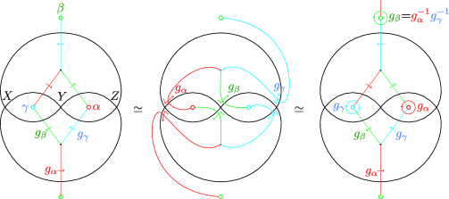
Figure 5. $\Theta$ whose associated $CF_{\hat{G}}(\mathbb{L},\mathbb{L})$ coincides with $CF(\mathbb{L},\mathbb{L};\hat{G})$ as algebras. (This is valid only for an abelian $G$. One of labelings in the bottom triangle should be replaced by its conjugate when $G$ is not abelian.)

Throughout, we use the presentation of $\pi_{1}(P)$ given as

$$\pi_{1}(P)=\langle g_{\alpha},g_{\beta},g_{\gamma}:g_{\alpha}g_{\beta}g_{\gamma}=1\rangle.$$

One of generators is redundant, but we prefer this symmetric expression which has a clear geometric origin as follows. In fact, the abelian group $G$ (the deck transformation of the abelian covering $X\to P$ in this context) is naturally a quotient of $\pi_{1}(P)$, and one can identify $g_{\alpha}$, $g_{\beta}$ and $g_{\gamma}$ with loops homotopic to $S_{\alpha}$, $S_{\beta}$ and $S_{\gamma}$ in 2.2 without ambiguity of the choice of a base point. Here, we use the same letters $g_{\alpha},g_{\beta},g_{\gamma}$ to denote the projections of the corresponding generators to $G$ (and we will do so from now on, when there is a no danger of confusion).

Furthermore, the Seidel Lagrangian $\mathbb{L}$ is liftable since, as a loop, its corresponding group element is conjugate to $g_{\gamma}g_{\beta}g_{\alpha}=g_{\beta}^{-1}g_{\alpha}^{-1}g_{\beta}g_{\alpha}$, and hence should be in the image of $p_{\ast}\pi_{1}(X)$ since $p$ is an abelian covering. Therefore our construction produces $CF_{\hat{G}}(\mathbb{L},\mathbb{L})$ whose $\hat{G}$-invariant part recovers $CF(\widetilde{\mathbb{L}},\widetilde{\mathbb{L}})$.

Lemma 3.11.

The obvious map

$$CF_{\hat{G}}(\mathbb{L},\mathbb{L})\to CF(\mathbb{L},\mathbb{L};\hat{G})$$

sending $Z\otimes\chi$ to the same expression on the right hand side precisely identifies the $A_{\infty}$-structure for $\Theta$ we have chosen above.

Proof.

Proof directly follows the picture. The middle diagram in Figure 5 shows an isotope of $\Theta$, and it has the following feature. Each time a path $\tau$ in $\mathbb{L}$ makes the turn at the odd/even-degree corner of $X$ (resp. $Y$ and $Z$), $g_{\tau}$ takes $g_{\alpha}$/$g_{\alpha}^{-1}$ (resp, $g_{\beta}^{\pm}$,$g_{\gamma}^{\pm}$) as its factor. Otherwise $g_{\tau}$ remains trivial since, for instance, if we pass through $X$ without making a turn, then $g_{\alpha}$ and $g_{\alpha}^{-1}$ cancel out. Therefore $g_{\tau}$ is obtained by multiplying of $g_{\alpha},g_{\beta},g_{\gamma}$ for each odd-degree $X$,$Y$,$Z$ in $\tau$ and multiplying their inverses for corresponding even corners in $\tau$. Notice its consistency with the $\hat{G}$-action on $CF(\mathbb{L},\mathbb{L})$:

$$\chi(X)=\chi(g_{\alpha}),\quad\chi(Y)=\chi(g_{\beta}),\quad\chi(Z)=\chi(g_{\gamma}),$$

$$\chi(\bar{X})=\chi(g_{\alpha}^{-1}),\quad\chi(\bar{Y})=\chi(g_{\beta}^{-1}),\quad\chi(\bar{Z})=\chi(g_{\gamma}^{-1}).$$

On the other hand, observe that the path $\gamma_{\beta,i}$ for a disk $u:(D^{2},\partial D^{2})\to(P,\mathbb{L})$ (in the $\beta\in\pi_{2}(P,\mathbb{L})$) is homotopic to the image under $u$ of the arc in $\partial D^{2}$ running from the $i$-th marked point to the $0$-th marked point. Therefore the factor $\chi_{i}(\gamma_{\beta,i})$ in $m_{k}(Z_{1}\otimes\chi_{1},\cdots,Z_{k}\otimes\chi_{k})$ on the left hand side $CF_{\hat{G}}(\mathbb{L},\mathbb{L})$ is nothing but the product $\chi_{i}(Z_{1})\cdots\chi_{i}(Z_{i})$, and hence $\prod_{i}\chi_{i}(\gamma_{\beta,i})$ recovers the twisting factor on $CF(\mathbb{L},\mathbb{L};\hat{G})$ appearing in (2.11). ∎

4. Orbifold mirror LG models for some punctured Riemann surfaces

In this section, we apply our earlier construction to the class of punctured Riemann surfaces $X$ whose quotient by a finite abelian group is isomorphic to the pair-of-pants $P$. For given such $X$, we prove that the symplectic cohomology of $X$ is naturally isomorphic to the orbifold LG B-model invariants defined in Section 2.3. The coincidence of the two closed-string invariants can also be shown by calculating both sides directly, for e.g. [GP20] for $SH(X)$. Here, we take more TQFT-oriented approach, as we will relate the two by an enumerative closed-open map, called the Kodaira-Spencer map in the spirit of [FOOO16].

Our strategy is first to establish the mirror symmetry for the pair-of-pants, and work equivariantly to deduce the analogous result for its abelian coverings. We begin with reviewing the construction of Kodaira-Spencer map, which is essentially a closed-open map applying to the single Lagrangian boundary.

There is another mirror construction of a general punctured Riemann surfaces by gluing local pieces isomorphic to $W=xyz$ according to some toric data determined by pair-of-pants decomposition of the surface (and its tropicalization). The resulting global mirror takes the form of a LG model on a toric Calabi-Yau 3-fold, which is actually a resolution of the orbifold LG mirror that we have here (for the case of abelian covers of the pair-of-pants.)

Remark 4.1.

Any finite abelian group $G=\mathbb{Z}/m\times\mathbb{Z}/n$ can serve as the deck transformation group of $X\to P$. By elementary covering theory, the genus $g$ of $X$ and its number of punctures $N$ in this case are related by

$$g=\frac{(m-1)(n-1)-\gcd(m,n)+1}{2}=\frac{mn-N}{2},\quad N=m+n+\gcd(m,n).$$ (4.1)

In particular, there are finitely many possible $N$ for a fixed $g$ if $g\geq 1$.

4.1. Kodaira-Spencer map

Let $X$ be a punctured Riemann surface with an abelian covering $\pi:X\to P$, and $\mathbb{L}$ the inverse image of the Seidel Lagrangian $\mathbb{L}$ in $X$ under $\pi$. We define one of main objects in our construction, the Kodaira-Spencer map, essentially as the closed-open map in [RS17] composed with the projection $HH^{\ast}(Fuk(X))\to HH^{\ast}(CF(\mathbb{L},\mathbb{L}))$,

$$SC^{\ast}(X)\to HH^{\ast}(Fuk(X))\to HH^{\ast}(CF(\mathbb{L},\mathbb{L}))$$ (4.2)

with some modification and reinterpretation of $HH^{\ast}(CF(\mathbb{L},\mathbb{L}))$ in the sense of Remark 2.11. The resulting map is also a noncompact analogue of the ring homomorphism appearing in [FOOO16] with the same name. Instead of working directly on $X$, we first pass to the quotient $P$ of $X$ and construct (4.2) for $P$, and recover that of $X$ using the equivariant construction in Section 3.

For this purpose, let us first review the construction of $\mathfrak{ks}:SC^{\ast}(P)\to CF((\mathbb{L},b),(\mathbb{L},b))$. (Of course, the construction can easily generalize to a more general situation as long as one can fulfill necessary technicalities.) For a fixed generic Morse function $f_{\mathbb{L}}$ on $\mathbb{L}$, let us consider the moduli space of maps $u$ consisting of the following data (see Figure 6 for their typical shapes):

• the main component $u_{0}:(D^{2}\setminus\{0\},\partial D^{2})\to(X,\mathbb{L})$ with one interior puncture (fixed to be the origin) and boundary marked points satisfying the Cauchy-Riemann equation perturbed by $H$ near the puncture and $J$-holomorphic away from this;

• finitely many $J$-holomorphic disks $u_{1},\cdots,u_{l}:(D^{2},\partial D^{2})\to(X,\mathbb{L})$ with boundary marked points;

• paths mapped to a negative gradient flow of $f_{\mathbb{L}}$ joining $u_{i}$ and $u_{j}$ for some $i$ and $j$ so that $u$ is continuous on the union of paths and disk components (which is connected and has no genus).

The data should satisfy

• $u_{0}$ is asymptotic to a Hamiltonian orbit in $SC^{\ast}(X)$ at the interior puncture;

• there exists a distinguished boundary marked point for the output, and the rest of boundary marked points are incident to $b=xX+yY+zZ$ where $x$, $y$ and $z$ are variables taking their values in $\Lambda_{+}$ as in 2.5;

• a path $\gamma_{u}$ from the interior puncture to the output is fixed (up to homotopy) for each $u$, which in particular determines the cylindrical parametrization near the puncture.

We denote by $\mathcal{M}_{CO}(\alpha,Z)$ the moduli space of $u$ satisfying the above and asymptotic to $\alpha$ and $Z$ at the interior puncture and the output marked point, respectively.

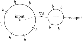
Figure 6. pearl trajectories counted for $\mathfrak{ks}$

Notice that this moduli is an adaption of the one in [RS17] for the Morse chain model on $CF(\mathbb{L},\mathbb{L})$. We remark that this does not create extra issues as long as one can guarantee the transversal intersection between the stable/unstable manifolds of the Morse function and the evaluation from the boundaries of disc components.

The count of elements in the moduli $\mathcal{M}_{CO}(\alpha,Z)$ (when it is rigid) gives rise to a map

$$\mathfrak{ks}:SC^{\ast}(P)\to CF((\mathbb{L},b),(\mathbb{L},b))$$

as usual, but we want to twist this analogously to operations on 3.2 and 3.7 (see (3.3), (3.4), (3.8)) so that it promotes to

$$\mathfrak{ks}_{\hat{G}}:SC_{\widehat{G}}^{\ast}(P)\to CF_{\hat{G}}((\mathbb{L},b),(\mathbb{L},b)).$$

This can be simply done by assigning the weight $g(\gamma_{u})$ to each $u$ in the moduli space, and define

$$\mathfrak{ks}_{\hat{G}}(\alpha\otimes\chi):=\sum_{u\in\mathcal{M}_{CO}(\alpha,Z)}\chi(g(\gamma_{u}))\,Z\otimes\chi.$$ (4.3)

As before, $g(\gamma_{u})$ only depends on the homotopy class of $u$.

Lemma 4.2.

$\mathfrak{ks}_{\hat{G}}$ is a $G\times\hat{G}$-equivariant dga map.

Proof.

The cobordism argument in [RS17] still works with additional consideration on the breaking of the Morse flow line which is already included as a part of $m_{1}$ on $CF((\mathbb{L},b),(\mathbb{L},b))$. Hence, we only need to check if $\mathfrak{ks}_{\hat{G}}$ is compatible with the twisted structure coming from the paths $\gamma$ from inputs to the output. This is purely a topological aspect, keeping track of (the homotopy classes) these paths under the degeneration. For example, to see $\mathfrak{ks}_{\hat{G}}$ is a chain map, we inspect the boundary behavior of elements in the 1-dimensional moduli $\mathcal{M}_{CO}(\alpha,Z)$. Possible degenerations are described in Figure 7.

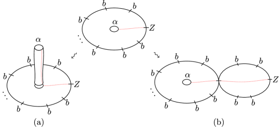
Figure 7. cobordism between $d_{\hat{G}}\circ\mathfrak{ks}_{\hat{G}}$ and $\mathfrak{ks}_{\hat{G}}\circ d_{\hat{G}}$ (when counted with weights coming from intersection between dotted paths and $\Theta$)

As in the proof of Lemma 2.1, one can make a coherent choice of $\gamma_{u}$ so that it is consistent with other choices of paths $\gamma$ from inputs to output for $SC_{\widehat{G}}^{\ast}(P)$ and $CF_{\hat{G}}((\mathbb{L},b),(\mathbb{L},b))$. Therefore the count of configurations in (a) of Figure 7 weighted by $\xi$ gives

$$\mathfrak{ks}_{\hat{G}}\circ d_{\hat{G}}(\alpha\otimes\chi)$$ (4.4)

whereas (b) of Figure 7 corresponds to

$$m_{1,\hat{G}}^{b\otimes 1,b\otimes 1}\circ\mathfrak{ks}_{\hat{G}}(\alpha\otimes\chi).$$ (4.5)

Notice that if a Floer cylinder $u$ attached with $v_{1}\in\mathcal{M}_{CO}(\alpha^{\prime},Z)$ is cobordant to $v_{2}\in\mathcal{M}_{CO}(\alpha,Z)$ with the bubbled-off disk $w$ through the cobordism in Figure 7, then the concatenation $\gamma_{u}\sharp\gamma_{v_{1}}$ is homotopic to $\gamma_{v_{2}}\sharp\gamma_{w}$. Therefore the weights $\xi(g_{u})$ in the counts (4.4) and (4.5) must agree. In general, the $1$-dimensional moduli can have more boundary components due to disk bubbles which do not contribute in our case due to weakly unobstructedness. Similar topological argument proves that $\mathfrak{ks}_{\hat{G}}$ preserves the product structure.

Recall that the $\hat{G}$ actions on both $SC_{\widehat{G}}^{\ast}(P)$ and $CF_{\hat{G}}((\mathbb{L},b),(\mathbb{L},b))$ are determined by the liftings of loops associated with generators. Then the $\hat{G}$-equvariance of $\mathfrak{ks}_{\hat{G}}$ is an easy consequence of the fact that for any $u\in\mathcal{M}_{CO}(\alpha,Z)$, the image (limit) of the interior puncture is homotopic to the image of the boundary. Obviously, $\mathfrak{ks}_{\hat{G}}$ is also $G$-equivariant with respect the $G$-action $g(\alpha\otimes\chi)=\chi(g)\alpha\otimes\chi$ and $g(Z\otimes\chi)=\chi(g)Z\otimes\chi$. ∎

Combined with Proposition 3.7 and 3.10, we obtain a natural map between $SH^{\ast}(X)$ and its closed-string $B$-invariant of the orbifold LG mirror, that is, the Koszul cohomology of $W$ relative to $\hat{G}$-action.

Corollary 4.3.

There exists a natural dga homomorphism $SC^{\ast}(X)\to CF((\tilde{\mathbb{L}},\tilde{b}),(\tilde{\mathbb{L}},\tilde{b}))$.

We conjecture that if $\mathfrak{ks}$ is a $\hat{G}$-equivariant quasi-isomorphism, then so is $\mathfrak{ks}_{\hat{G}}$.

4.2. Pair-of-pants and its mirror potential $W(x,y,z)=xyz$

Let us first look into the pair-of-pants $P$, which will serve as a building block for subsequent cases. Recall from 2.2 that the symplectic cohomology ring $SH^{\ast}(P)$ admits the following representation

$$SH^{\ast}(P)=\Bbbk\langle e\rangle\oplus\Bbbk\langle f_{1}\rangle\oplus\Bbbk\langle f_{2}\rangle\oplus\Bbbk\langle e_{\alpha},f_{\alpha}\rangle[t_{\alpha}]\oplus\Bbbk\langle e_{\beta},f_{\beta}\rangle[t_{\beta}]\oplus\Bbbk\langle e_{\gamma},f_{\gamma}\rangle[t_{\gamma}]$$

with the product structure determined by

$$f_{1}\star e_{\alpha}=f_{\alpha},\quad e_{\alpha}\star e_{\alpha}=e_{\alpha},\quad e_{\alpha}\star f_{\alpha}=f_{\alpha}$$

$$f_{1}\star e_{\beta}=f_{2}\star e_{\beta}=f_{\beta},\quad e_{\beta}\star e_{\beta}=e_{\beta},\quad e_{\beta}\star f_{\beta}=f_{\beta}$$

$$f_{2}\star e_{\gamma}=f_{\gamma},\quad e_{\gamma}\star e_{\gamma}=e_{\gamma},\quad e_{\gamma}\star f_{\gamma}=f_{\gamma}$$

and the products between different $t_{a}$’s vanish. Geometrically, $e$(serving as the unit), $f_{i}$ are Morse generators appearing in $P^{in}$ and $e_{\alpha}t_{\alpha}^{l}$ and $f_{\alpha}t_{\alpha}^{l}$ are Hamiltonian oribits around one of the punctures with winding number $l$ (and similar for $\beta$ and $\gamma$).

Let us now consider the LG mirror of $P$. As before, we take $\mathbb{L}$ to be the Seidel Lagrangian, whose Maurer-Cartan deformation induces the mirror LG-model $W:\Bbbk^{3}\to\Bbbk,W(x,y,z)=xyz$. The coefficient ring $\Bbbk$ will be $\mathbb{C}$ in the mirror symmetry consideration. We take the Koszul complex $(K^{\ast}(\partial W),d_{W})$ defined in 2.3 (with trivial $H$) as the associated closed-string B-model, in this case, consisting of the following data:

$$K^{\ast}(\partial W) =S_{R}^{\bullet}\left(\bigoplus_{t\in\{x,y,z\}}R\cdot\theta_{t}\right),$$

$$d_{W} =yz\partial_{\theta_{x}}+zx\partial_{\theta_{y}}+xy\partial_{\theta_{z}}.$$

where $R=\Bbbk[x,y,z]$ is the function ring of $\Bbbk^{3}$ and $\theta_{a}$’s for $a\in\{x,y,z\}$ are formal variables of degree $-1$ as before. (The exterior degree here is for the convenience of exposition, and we will only use its reduced $\mathbb{Z}/2$-grading, later.)

The degree $-3$ component is $R\cdot\theta_{x}\theta_{y}\theta_{z}$, and it injects into the $-2$-degree component under $d_{W}$ since $R$ is an integral domain. Therefore its cohomology at degree $-3$ vanishes. For the cohomology at degree $-2$, suppose $\omega=f_{x}\theta_{y}\theta_{z}+f_{y}\theta_{z}\theta_{x}+f_{z}\theta_{x}\theta_{y}$ is a cocycle, i.e.,

$$d_{W}(\omega)=x(yf_{y}-zf_{z})\theta_{x}+y(zf_{z}-xf_{x})\theta_{y}+z(xf_{x}-yf_{y})\theta_{z}=0.$$

It leads to $xf_{x}=yf_{y}=zf_{z}$ which we denote by $f$. Since $xyz$ divides $f$, we may write $f=xyzg$. Then we have $f_{x}=yzg$, $f_{y}=zxg$, and $f_{z}=xyg$ so that

$$\omega=g(yz\theta_{y}\theta_{z}+zx\theta_{z}\theta_{x}+xy\theta_{x}\theta_{y})=d_{W}(g\theta_{x}\theta_{y}\theta_{z}).$$

Thus the $-2$nd cohomology is also zero.

In order to compute the cohomology in degree $-1$, it is elementary to check that $\lambda=g_{x}\theta_{x}+g_{y}\theta_{y}+g_{z}\theta_{z}$ is cocycle if and only if it is a $R$-linear combination of $\lambda_{x}=y\theta_{y}-z\theta_{z}$, $\lambda_{y}=z\theta_{z}-x\theta_{x},$ and $\lambda_{z}=x\theta_{x}-y\theta_{y}$. These generators satisfy the single linear relation $\lambda_{x}+\lambda_{y}+\lambda_{z}=0$ (on the chain level). On the other hand, the set of coboundaries is spanned by $x\lambda_{x}$, $y\lambda_{y}$, and $z\lambda_{z}$. Therefore the $(-1)$-cohomology is given as

$$H^{-1}(K^{\ast}(\partial W))=\dfrac{\{h_{x}\lambda_{x}+h_{y}\lambda_{y}+h_{z}\lambda_{z}:h_{x},\,h_{y},\,h_{z}\in R\}}{\langle x\lambda_{x}=y\lambda_{y}=z\lambda_{z}=0\rangle}=\dfrac{\{h_{x}\lambda_{x}+h_{y}\lambda_{y}:h_{x},h_{y}\in R\}}{\langle x\lambda_{x}=y\lambda_{y}=0\rangle}$$

where we used $\lambda_{x}+\lambda_{y}+\lambda_{z}=0$ at the end.

On the cohomology, we have the following induced relations

$$\begin{array}[]{c}yz\lambda_{x}=0,\quad zx\lambda_{y}=0,\quad xy\lambda_{z}=0,\\[2.0pt] x^{i}\lambda_{y}=-x^{i}\lambda_{z},\quad y^{i}\lambda_{z}=-y^{i}\lambda_{x}\quad z^{i}\lambda_{x}=-z^{i}\lambda_{y}\end{array}$$

for $i\geq 1$ that completely determine the $R$-module structure on $H^{-1}(K^{\ast}(\partial W))$, which descends to $R/\langle yz,zx,xy\rangle$-module structure. We also have the relations

$$\begin{array}[]{c}\lambda_{x}^{2}=\lambda_{y}^{2}=\lambda_{z}^{2}=0,\quad\lambda_{y}\lambda_{z}=\lambda_{z}\lambda_{x}=\lambda_{x}\lambda_{y}=d_{W}(\theta_{x}\theta_{y}\theta_{z}).\end{array}$$ (4.6)

Finally, because $K^{-1}(\partial W)=\bigoplus_{a\in\{x,y,z\}}R\cdot\theta_{a}$ whereas $K^{0}(\partial W)$ is simply $R$, we find that $H^{0}(K^{\ast}(\partial W))=R/\langle yz,zx,xy\rangle$. Consequently,

$$Kos(W)=H^{\ast}(K^{\ast}(\partial W)) = H^{0}(K^{\ast}(\partial W))\oplus H^{-1}(K^{\ast}(\partial W))$$

$$\cong R/\langle yz,zx,xy\rangle\oplus\dfrac{\{h_{x}\lambda_{x}+h_{y}\lambda_{y}:h_{x},h_{y}\in R\}}{\langle x\lambda_{x}=y\lambda_{y}=0\rangle},$$

and it has a structure of $H^{0}(K^{\ast}(\partial W))$-module which is generated by $1_{R}\in H^{0}(K^{\ast}(\partial W))$ and by $\lambda_{x},\lambda_{z}\in H^{-1}(K^{\ast}(\partial W))$ subject to the algebra relations

$$\begin{array}[]{c}x\lambda_{x}=z\lambda_{z}=0,\quad y\lambda_{x}=-y\lambda_{z},\quad\lambda_{x}^{2}=\lambda_{z}^{2}=\lambda_{x}\lambda_{z}=\lambda_{z}\lambda_{x}=0.\end{array}$$

Under the identification $\Theta$ in Proposition 2.15, the above generators correspond to

$$1_{R},\quad\lambda_{x},\quad\lambda_{z}\qquad\longleftrightarrow\qquad e_{\mathbb{L}},\quad yY-zZ,\quad xX-yY$$

in $CF((\mathbb{L},b),(\mathbb{L},b))$.

From the above explicit descriptions, we see that there is an obvious ring isomorphism between $SH(P)$ and $Kos(W)$, which matches generators of $SH(P)$ and those of $Kos(W)=H^{\ast}(K^{\ast}(\partial W))$ via

$$\begin{array}[]{c}e\mapsto 1_{R},\quad e_{\alpha}t_{\alpha}^{i}\mapsto x^{i},\quad e_{\beta}t_{\beta}^{i}\mapsto y^{i},\quad e_{\gamma}t_{\gamma}^{i}\mapsto z^{i},\\[3.0pt] f_{1}\mapsto\lambda_{z},\quad f_{2}\mapsto\lambda_{x}\end{array}$$

for all $i\geq 1$. Observe that we have chosen generators on both sides in such a way that relations among them precisely match. The only remaining question is now if the Kodaira-Spencer map $\mathfrak{ks}:SH(P)\to CF((\mathbb{L},b),(\mathbb{L},b))$ composed with the qausi-isomorphism $CF((\mathbb{L},b),(\mathbb{L},b))\to K^{\ast}(\partial W)$ geometrically realizes this. We have $\mathfrak{ks}(e)=e_{\mathbb{L}}$ since the closed-open map is unital, and $e_{\mathbb{L}}$ again maps to the unit in $K^{\ast}(\partial W)$. Observing that $SH(P)$ is (multiplicatively) generated by $e_{\alpha}t_{\alpha}$, $e_{\beta}t_{\beta}$, $e_{\gamma}t_{\gamma}$, $f_{1}$ and $f_{2}$, it now suffices to determine their images under $\mathfrak{ks}$.

Lemma 4.4.

The Kodaira-Spencer map $\mathfrak{ks}:SC(P)\to CF((\mathbb{L},b),(\mathbb{L},b))$ computes

$$\begin{array}[]{c}\mathfrak{ks}(e_{\alpha}t_{\alpha})=x\,e_{\mathbb{L}},\quad\mathfrak{ks}(e_{\beta}t_{\beta})=y\,e_{\mathbb{L}},\quad\mathfrak{ks}(e_{\gamma}t_{\gamma})=z\,e_{\mathbb{L}}\\[3.0pt] \mathfrak{ks}(f_{1})=-xX+yY,\quad\mathfrak{ks}(f_{2})=-yY+zZ.\end{array}$$

Proof.

By obvious symmetry, it suffices to deal with the case for $\alpha$. We first show $\mathfrak{ks}(e_{\alpha}t_{\alpha})=xe_{\mathbb{L}}$. Note that the geometric representative of $e_{\alpha}t_{\alpha}$ is topologically a simple close curve round the puncture $\alpha$. It is easy to find a pair of topological (punctured) disks $u$ and $u^{\prime}$ whose punctured boundary in the interior wraps $\alpha$ exactly once and the boundary circle hits the corner $X$. (Figure 8)

Figure 8. Two punctured disks for $\mathfrak{ks}(e_{\alpha}t_{\alpha})$

To see that these can be realized as genuine pseudo-holomorphic curves, take a contact hypersurface $C$ that is a circle enclosing $\alpha$ contained inside the disk. Making use of the domain-stretching argument in [Ton19, 5.2] with respect to $C$ depicted in Figure 9, one can show that these topological disks actually admit parametrizations satisfying the (perturbed) Cauchy-Riemann equation, and that they are the only ones that possibly contribute to $\mathfrak{ks}(e_{\alpha}t_{\alpha})$. It amounts to exclude undesirable orbits that may happen in the breaking region. See [CCJv1, Proposition 9.5] for more details. Alternatively, one can also apply more tradition neck-stretching argument (that degenerates the almost complex structure) to split the disk $u$ into $u_{1}$ and $u_{2}$ and compactify each using the finiteness of the energy. $u_{1}$ becomes a Maslov $2$ disk bounding $\mathbb{L}$ in the compactification of $P$ where $u_{2}$ is a pseudo-holomorphic cylinder appearing in the calculation of $d$ on $SC^{\ast}(\mathbb{C})$ (the degree of $\alpha$ as an orbit in $\mathbb{C}$ is odd).

Figure 9. SFT-strectching

Clearly $u$ contributes $xe_{\mathbb{L}}$ to $\mathfrak{ks}(e_{\alpha}t_{\alpha})$. On the other hand, both $u$ and $u^{\prime}$ can be viewed as punctured disks with the output $\bar{X}$. Calculating signs carefully, these contributions turn out to cancel each other. Factors contributing to their signs appear in [Abo10, Lemma C.4] in details, and in fact, the nontrivial spin structure put on $\mathbb{L}$ is solely responsible for their opposite signs in our case. This is no longer the case if we twist operations with weights induced from $\gamma_{u}$ and $\gamma_{u^{\prime}}$ in Figure 8, in the presence of a nontrivial $\hat{G}$-action.

We next compute $\mathfrak{ks}(f_{1})$. By degree reason (in terms of fractional grading) and by $G$-equivariance of $\mathfrak{ks}$, $\mathfrak{ks}(f_{1})$ must be a linear combination of $xX$, $yY$, $zZ$ and $f_{\mathbb{L}}$. Comparing the actions, we see that $\mathfrak{ks}(f_{1})$ can have contributions only from Morse trajectories and constant disks. Suppose it is given as

$$\mathfrak{ks}(f_{1})=c_{x}xX+c_{y}yY+c_{z}zZ+c_{f_{\mathbb{L}}}f_{\mathbb{L}}$$

for some coefficients $c_{x},c_{y},c_{z}$ and $c_{f_{\mathbb{L}}}$ in $\mathbb{C}$. Firstly, it is immediate to see there are exactly two cascades from $f_{1}$ to $f_{\mathbb{L}}$. They are the concatenated paths consisting of Morse trajectories of the Morse function on $\mathbb{L}$ and those of the ambient Morse function joined at $r$ and $s$ respectively. See (b) of Figure 11. They have the opposite signs due to the intersection parities of two trajectories at $r$ and $s$. Thus we have $c_{f_{\mathbb{L}}}=0$.

To find the remaining coefficients $c_{x},c_{y},c_{z}$, we argue as follows. Choose an abelian quotient $G$ of $\pi_{1}(P)$ of the shape $G=\langle g_{\alpha},g_{\beta},g_{\gamma}:g_{\alpha}^{n}=g_{\alpha}g_{\beta}=g_{\gamma}=1\rangle\cong\mathbb{Z}/n$, and consider the corresponding principal $G$-bundle $X\to P$. With respect to $\Theta$ chosen in Figure 11 (a) and a nontrivial $\chi\in\hat{G}$, we compute the differential on $SC(P)\otimes\chi(\subset SC_{\widehat{G}}(P))$ and $CF((\mathbb{L},b),(\mathbb{L},b))\otimes\chi(\subset CF((\mathbb{L},b),(\mathbb{L},b);\hat{G}))$. The coefficients $c_{x},c_{y},c_{z},$ will be determined by comparison. Observe first that

$$d_{{\widehat{G}}}(e\otimes\chi)=\chi(g_{\beta})(1-\chi(g_{\alpha}))f_{1}\otimes\chi=\left(\chi(g_{\alpha}^{-1})-1\right)f_{1}\otimes\chi$$

by looking at the intersections of two isolated Morse trajectory from $e$ to $f_{1}$ (for the ambient Morse function) with $\Theta$. Taking $\mathfrak{ks}_{{\widehat{G}}}$ on both sides yields

$$\mathfrak{ks}_{{\widehat{G}}}\left(d_{{\widehat{G}}}(e\otimes\chi)\right)=\left(\chi(g_{\alpha}^{-1})-1\right)\mathfrak{ks}_{{\widehat{G}}}(f_{1}\otimes\chi).$$ (4.7)

Since $\mathfrak{ks}_{\hat{G}}$ is a chain map, the left hand side of (4.7) becomes

$$\begin{split}\mathfrak{ks}_{{\widehat{G}}}\left(d_{{\widehat{G}}}(e\otimes\chi)\right)&=m_{1,{\widehat{G}}}^{b\otimes 1,b\otimes 1}\left(\mathfrak{ks}_{{\widehat{G}}}(e\otimes\chi)\right)\\ &=m_{1,{\widehat{G}}}^{b\otimes 1,b\otimes 1}\left(\chi(g_{\alpha}^{-1})e_{\mathbb{L}}\otimes\chi\right)\\ &=\chi(g_{\alpha}^{-1})\left(\left(1-\chi(g_{\alpha}^{-1})\right)xX\otimes\chi+\left(1-\chi(g_{\alpha})\right)yY\otimes\chi\right)\\ &=\left(1-\chi(g_{\alpha}^{-1})\right)\left(\chi(g_{\alpha}^{-1})xX\otimes\chi-yY\otimes\chi\right)\end{split}$$

where we used $\mathfrak{ks}_{{\widehat{G}}}(e\otimes\chi)=\chi(g_{\alpha}^{-1})e_{\mathbb{L}}\otimes\chi$ in the middle, which can be easily seen from the intersection of the ambient Morse trajectory from $e$ to $e_{\mathbb{L}}$ with $\Theta$.

We now compute the right hand side of (4.7), $\mathfrak{ks}_{{\widehat{G}}}(f_{1}\otimes\chi)$. By definition, it counts exactly the same pearl trajectories as those for $\mathfrak{ks}(f_{1})$, but with weights coming from the intersection with $\Theta$. Notice that in either cases, contributing trajectories must lie inside the colored Morse trajectories in Figure 11 (b), considering the locations of input and outputs. Keeping track of intersection patterns of these two with $\Theta$, we can compare easily the difference between $\mathfrak{ks}(f_{1})$ and $\mathfrak{ks}_{{\widehat{G}}}(f_{1}\otimes\chi)$, and it results in

$$\mathfrak{ks}_{{\widehat{G}}}(f_{1}\otimes\chi)=\chi(g_{\alpha}^{-1})c_{x}xX\otimes\chi+c_{y}yY\otimes\chi+c_{z}zZ\otimes\chi.$$

Equating this with $-\chi(g_{\alpha}^{-1})xX\otimes\chi+yY\otimes\chi$ from the left hand side, we have $c_{x}=-1$, $c_{y}=1$ and $c_{z}=0$. ∎

Consequently, we see that $\mathfrak{ks}$ is a quasi-isomorphism:

Corollary 4.5.

$\mathfrak{ks}$ induces a ring isomorphism $SH(P)\to HF((\mathbb{L},b),(\mathbb{L},b))$, and hence that between $SH(P)$ and $Kos(W)$ due to Proposition 2.13 (with $H=1$).

Proof.

Recall that both $SH^{0}(P)$ and $HF^{0}((\mathbb{L},b),(\mathbb{L},b))$ are isomorphic to the function ring of the union of three coordinate axes in $\mathbb{C}^{3}$. Both $SH(P)$ and $HF((\mathbb{L},b),(\mathbb{L},b))$ can be regarded as finitely generated modules over $\mathbb{C}[x,y,z]/\langle xy,yz,zx\rangle$, and Lemma 4.4 identifies the module generators (see (2.2) and (2.15)). From (2.3) and (2.16), product relations among these generators also match. ∎

It is worthwhile to mention that $\mathfrak{ks}$ intertwines algebraic and geometric relations in $SH(P)$ and $HF((\mathbb{L},b),(\mathbb{L},b))$. For example, we have $f_{1}\cdot f_{2}=0$ on the chain level (in $SC^{\ast}(P)$) since there is no contributing holomorphic curves, but there is a geometric relation $m_{2}(xX-yY,zZ-xX)=m_{1}^{b,b}(f_{\mathbb{L}})$ from disk counting on the other side. Thus $m_{2}(\mathfrak{ks}(f_{1}),\mathfrak{ks}(f_{2}))=0$ holds only on the cohomology.

4.3. Abelian covers of pair-of-pants and orbifold LG mirror

We now establish the closed string mirror symmetry for an abelian cover $X$ of $P=X/G$ based on the quasi-isomorphism $\mathfrak{ks}$, or more precisely, by orbifolding $\mathfrak{ks}$ with respect to $\hat{G}$-action. Throughout, we work with the geometric setup given in (a) of Figure 11. In particular, relative positions of $\Theta$ and Floer generators are fixed. Notice that $\Theta$ here is a Borel-Moore cycle and is different from our earlier choice in 3.4. Figure 10 shows the isotopy between the two not crossing self-intersections of $\mathbb{L}$, and hence they result in the same calculation. We then have the following.

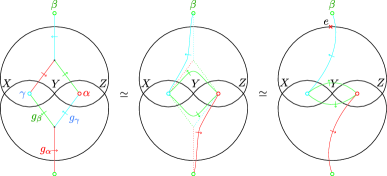
Figure 10. Deforming $\Theta$ on $P$ given in Figure 5

Theorem 4.6.

The dga homorphism

$$\mathfrak{ks}_{{\widehat{G}}}:SC_{\widehat{G}}^{\ast}(P)\to CF_{{\widehat{G}}}((\mathbb{L},b),(\mathbb{L},b))$$

defined in 4.3 gives a $G\times{\widehat{G}}$-equivariant quasi-isomorphism.

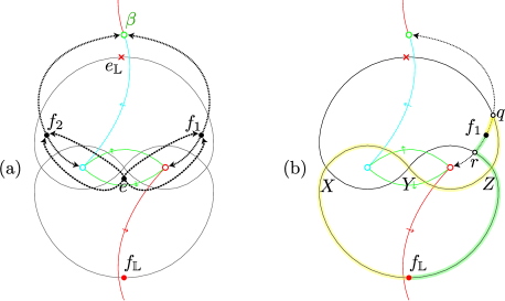
Figure 11. Choice of Morse functions and their trajectories contributing to $\mathfrak{ks}_{\hat{G}}$

Proof.

Since we know $\mathfrak{ks}_{{\widehat{G}}}$ preserves the product structure, it suffice to prove that the composition below is a quasi-isomorphism of complexes

in each $\chi$-sector $SC^{\ast}(P)\otimes\chi$. We denote this composition by $\mathcal{F}\otimes\chi$. The case where $\chi=1$ corresponds to the pair-of-pants $P$ itself, which is shown in Corollary 4.5. Assume $\chi\neq 1$ for the rest of the proof.

We first claim that the part of $SC^{\ast}(P)\otimes\chi$ generated by Morse critical points $e\otimes\chi$, $f_{1}\otimes\chi$ and $f_{2}\otimes\chi$ gives rise to an 1-dimensional cohomology in the odd degree. To see this, we count the gradient trajectories $\gamma_{i}$ and $\delta_{i}$ in Figure 10 between these generators $e$ and $f_{i}$, but with the weights determined by their intersections with $\Theta$ (due to the effect of twisting in the $\chi$-sector). By direct calculations

$$d(e\otimes\chi)=\pm\left(\chi(\gamma_{1})-\chi(\delta_{1})\right)f_{1}\otimes\chi\pm\left(\chi(\gamma_{2})-\chi(\delta_{2})\right)f_{2}\otimes\chi.$$

This is always nonzero for $\chi\neq 1$ since $\gamma_{1}\ast\delta_{1}^{-}$, $\gamma_{2}\ast\delta_{2}^{-}$ generate the first homology of $P$. Hence $e\otimes\chi$ does not support a cocycle in this case, and $f_{1},f_{2}$ are colinear in the cohomology.

Let us next consider non-contractible loops of $SC^{\ast}(P)\otimes\chi$. We only have possibly nontrivial Floer differential between the elements of the form $e_{\alpha}t_{\alpha}^{n}\otimes\chi$ and $f_{\alpha}t_{\alpha}^{n}\otimes\chi$ (and similar for $\beta$ and $\gamma$) since otherwise there does not exist any contributing Floer cylinders. There are exactly two holomorphic cylinders $u,v$ whose two ends asymptote $e_{\alpha}t_{\alpha}^{n}\otimes\chi$ (input) and $f_{\alpha}t_{\alpha}^{n}\otimes\chi$ (output) or their underlying orbits. The contributions of the two cylinders $u,v$ cancel in the absence of $\chi$, so both $e_{\alpha}t_{\alpha}^{n}$ and $f_{\alpha}t_{\alpha}^{n}$ survive in $SH^{\ast}(P)$. However, the twisted differential of $SC^{\ast}(P)\otimes\chi$ applied to $e_{\alpha}t_{\alpha}^{n}\otimes\chi$ gives $\pm(\chi(\gamma_{u})-\chi(\gamma_{v}))f_{\alpha}t_{\alpha}^{n}\otimes\chi$, and $\chi(\gamma_{u})-\chi(\gamma_{v})=0$ if and only if $\chi(\gamma_{u}\ast\gamma_{v}^{-})=\chi(\alpha)=1$ (since $\gamma_{u}\ast\gamma_{v}^{-}$ or its reverse is homotopic to $\alpha$, see [CFHW96, Section 2] for more details).

To summarize, $SH^{\ast}(P)\otimes\chi$ takes a single generator in degree $1$ from the Morse part for $\chi\neq 1$, and takes two generators $e_{\alpha}t_{\alpha}^{n}\otimes\chi$ and $f_{\alpha}t_{\alpha}^{n}\otimes\chi$ ($n\geq 1$) if and only if $\chi(g_{\alpha})=1$, and similar for $\beta$ and $\gamma$. Let us now look into the behavior of $\mathfrak{ks}_{{\widehat{G}}}$ on these generators. We divide our proof into two cases depending on the action of $\chi$ on three variables $x$, $y$ and $z$.

Case 1. When $\chi$ fixes at least one of $x$, $y$, and $z$:
Without loss of generality, we assume $\chi\cdot x=x$. As seen above, there are exactly two nonzero cohomology classes $e_{\alpha}t_{\alpha}^{n}\otimes\chi$ and $f_{\alpha}t_{\alpha}^{n}\otimes\chi$ (of degrees 0 and 1, respectively) belonging to the free loop class $\alpha^{n}$ for each $n\geq 1$. Summing up over all $n\geq 1$ and adjoining $f_{1}\otimes\chi$, they form a free $\mathbb{C}e\oplus e_{\alpha}t_{\alpha}\mathbb{C}[t_{\alpha}]$-module of rank $2$, generated by $e_{\alpha}t_{\alpha}\otimes\chi$ and $f_{1}\otimes\chi$ in degree $0$ and $1$. Here, $\mathbb{C}e\oplus e_{\alpha}t_{\alpha}\mathbb{C}[t_{\alpha}]$ means $(\mathbb{C}e\oplus e_{\alpha}t_{\alpha}\mathbb{C}[t_{\alpha}])\otimes 1(\subset SH(P;\hat{G})$), but we omit $-\otimes 1$ for notational simplicity.

The module structure is induced from the product on $SH(P;\hat{G})$, and more specifically, it is given as

$$(e_{\alpha}t_{\alpha}^{n}\otimes 1)\cdot(e_{\alpha}t_{\alpha}\otimes\chi)=e_{\alpha}t_{\alpha}^{n+1}\otimes\chi,\quad(e_{\alpha}t_{\alpha}^{n}\otimes 1)\cdot(f_{1}\otimes\chi)=(f_{\alpha}t_{\alpha}^{n})\otimes\chi$$

where $e_{\alpha}t_{\alpha}^{n-1}\otimes 1$ and $e_{\alpha}t_{\alpha}^{n-1}$ in $\mathbb{C}e\oplus e_{\alpha}t_{\alpha}\mathbb{C}[t_{\alpha}]$ are identified. Observe that the ring $\mathbb{C}e\oplus e_{\alpha}t_{\alpha}\mathbb{C}[t_{\alpha}]$ is nothing but a polynomial ring in $1$-variable, and in fact, it maps to $\mathbb{C}[x]$ under $\mathcal{F}\otimes 1$ .

On the other hand, $\mathbb{C}[x,y,z]^{\chi}=\mathbb{C}[x]$ in this case, so the Koszul complex $K^{\ast}(\partial W^{\chi})$ is a $\mathbb{C}[x]$-module in the following form:

Hence its cohomology $Kos(W,\chi)$ is a free $\mathbb{C}[x]$-module of rank $1$ in each degree ($0$ or $1$). It is freely generated by any nonzero multiples of $\theta_{x}\theta_{y}\theta_{z}$ and $\theta_{y}\theta_{z}$ in degree $1$ and $0$, respectively.

Pseudo-holomorphic curves contributing to $\mathfrak{ks}_{\hat{G}}(e_{\alpha}t_{\alpha}\otimes\chi)$ are already classified in the proof of Lemma 4.4. Additional factor here is the nontrivial weight coming from the intersection between $\Theta$ and $\gamma_{u}$ or $\gamma_{u^{\prime}}$. Take these into account, we obtain

$$\mathfrak{ks}_{\hat{G}}(e_{\alpha}t_{\alpha}\otimes\chi)=\pm(\chi(g_{\beta})-1)\bar{X}\otimes\chi\pm x\,e_{\mathbb{L}}\otimes\chi.$$ (4.8)

After mapped under $\tau$ in (2.18), only the first term in (4.8) survives, and becomes a nonzero multiple of $\theta_{y}\theta_{z}$ since $\chi(g_{\beta})\neq 1$.

Let us now compute $\mathfrak{ks}_{\hat{G}}(f_{1}\otimes\chi)$. Considering the behavior of $\tau$ in (2.18), it suffice to prove that the coefficient of $f_{\mathbb{L}}\otimes\chi$ in $\mathfrak{ks}_{\hat{G}}(f_{1}\otimes\chi)$ is nonzero (so that $f_{1}\otimes\chi$ maps to a nonzero multiple of $\theta_{x}\theta_{y}\theta_{z}$ under $\mathcal{F}\otimes\chi$.) Contributions are from two (concatenated) morse trajectories marked in 11 (b). Tracking the intersections of these trajectories with $\Theta$, we have

$$\mathfrak{ks}_{\hat{G}}(f_{1}\otimes\chi)=\pm(1-\chi(g_{\gamma}))f_{\mathbb{L}}\otimes\chi\pm AyY\otimes\chi\pm BxX\otimes\chi,$$ (4.9)

and we see that the coefficient of $f_{\mathbb{L}}\otimes\chi$ is nonzero as desired. (They cancel each other when $\chi=1$ as seen in the proof of Lemma 4.4.) Consequently, $\mathcal{F}\otimes\chi$ matches sets of free generators of two free modules over $\mathbb{C}e\oplus e_{\alpha}t_{\alpha}\mathbb{C}[t_{\alpha}]$ and $\mathbb{C}[x]$ which are identified as rings by $\mathcal{F}\otimes 1$, and hence, is an isomorphism.

Case 2. When $\chi$ fixes none of $x$, $y$, and $z$:
We have $\mathbb{C}[x,y,z]^{\chi}=\mathbb{C}$ and the Koszul complex is the free module generated by $\theta_{x}\theta_{y}\theta_{z}$ over $\mathbb{C}$. Also, non-contractible orbits cannot become a cocycle in $SC^{\ast}(P)\otimes\chi$ as we have examined above. Thus the only cohomology generator of $SH^{\ast}(P)\otimes\chi$ is of degree 1, represented by the class $f_{1}\otimes\chi$ or $f_{2}\otimes\chi$. As in $\eqref{eqn:ksf1}$, $\mathfrak{ks}_{{\widehat{G}}}(f_{1}\otimes\chi)$ has a nonzero coefficient for $f_{\mathbb{L}}\otimes\chi$ term (since $\chi(g_{\gamma})\neq 1$), and maps to a nonzero multiple of $\theta_{x}\theta_{y}\theta_{z}$ under $\mathcal{F}\otimes\chi$, which completes the proof. ∎

The following is an immediate consequence of $G\times{\widehat{G}}$-equivariance of $\mathfrak{ks}_{{\widehat{G}}}$.

Corollary 4.7.

The Kodaira-Spencer map restricts to a $G$-equivariant quasi-isomorphism (of dgas)

$$\mathfrak{ks}_{{\widehat{G}}}:\left(SC_{\widehat{G}}^{\ast}(P)\right)^{{\widehat{G}}}\to\left(CF_{{\widehat{G}}}((\mathbb{L},b),(\mathbb{L},b))\right)^{{\widehat{G}}}$$

on ${\widehat{G}}$-invariant parts of both sides. Therefore we obtain an isomorphism

$$SH(X)\cong Kos(W,\hat{G})$$

as modules.

We can also equip $Kos(W,\hat{G})$ with the product structure by transferring $m_{2,\hat{G}}^{b\otimes 1,b\otimes 1,b\otimes 1}$ on $H^{\ast}\left(CF_{{\widehat{G}}}((\mathbb{L},b),(\mathbb{L},b))\right)^{{\widehat{G}}}$ in this case. Corollary 4.7 justifies the new product structure in the mirror symmetry context. More general treatment will be provided elsewhere. The explicit formula for the differential on $CF_{{\widehat{G}}}((\mathbb{L},b),(\mathbb{L},b))$ is presented in Appendix A as well as one convenient choice of generators for its cohomology (which is an infinite dimensional vector space over $\mathbb{C}$).

4.4. Examples

We end our discussion with simple examples that manifest the feature of the effect of orbifolding. The following are the examples whose mirrors are heuristically explained in Introduction (see Figure 1 and Figure 2). Here, we give a precise formulation of their orbifold LG mirrors.

4.4.1. Sphere with four punctures

Suppose $X$ is a sphere with four punctures. It admits the rotation action of $G=\mathbb{Z}/2$ whose quotient is the pair-of-pants $P$. As the deck transformation group, $G$ can be identified as the quotient of $\pi_{1}(P)$ as

$$\langle g_{\alpha},g_{\beta},g_{\gamma}:g_{\alpha}^{2}=g_{\alpha}g_{\beta}=g_{\gamma}=1\rangle.$$

In the character group ${\widehat{G}}$, we have a unique non-unit $\chi$ whose value on the generator $g_{\alpha}=g_{\beta}$ is equal to $-1$. This specializes the situation in “case 1” in the proof of Theorem 4.6. On the mirror side, the nontrivial twisted sector $Kos(W,\chi)$ is given by

$$\mathbb{C}[z]\theta_{x}\theta_{y}\oplus\mathbb{C}[z]\theta_{x}\theta_{y}\theta_{z}.$$

Note that this is precisely the (algebraic) de Rham complex of $\mathbb{C}$ (with coordinate $z$) up to degree shift which appear in Figure 2 (b). In terms of $CF((\mathbb{L},b),(\mathbb{L},b))\otimes\chi$, $\theta_{x}\theta_{y}$ and $\theta_{x}\theta_{y}\theta_{z}$ correspond to

$$\bar{Z}\otimes\chi+\frac{1}{2}z\,e_{\mathbb{L}}\otimes\chi,\quad\,f_{\mathbb{L}}\otimes\chi+\frac{1}{2}(yY\otimes\chi+zZ\otimes\chi).$$

One can compute the new product structure on $Kos(W,\hat{G})$ using these representatives in the Floer complex or using their corresponding elements in $SH(X)$ (see Appendix B).

4.4.2. Torus with three punctures

Let us now take $X$ to be a torus with three punctures. The deck transformation group of $X\to P$ can be presented as

$$G=\langle g_{\alpha},g_{\beta},g_{\gamma}:g_{\alpha}^{3}=g_{\beta}^{3}g_{\gamma}^{3}=g_{\alpha}g_{\beta}g_{\gamma}=1\rangle,$$

and choose $\chi\in G$ such that $\chi(g_{\alpha})=\chi(g_{\beta})=\chi(g_{\gamma})=\rho$ where $\rho=e^{2\pi i/3}\in\mathbb{C}$. This specializes “case 2” in the proof of Theorem 4.6.

In this case, we have a twist sector for each of $\chi$ and $\chi^{2}$. Since there are no invariant variables, twisted sectors are given as

$$Kos(W,\chi)=\mathbb{C}\,\theta_{x}\theta_{y}\theta_{z},\quad Kos(W,\chi^{2})=\mathbb{C}\,\theta_{x}\theta_{y}\theta_{z}.$$

These correspond to the two additional points in Figure 2 (b).

In terms of $CF((\mathbb{L},b),(\mathbb{L},b);\hat{G})^{\hat{G}}$, these two sectors can be more clearly distinguished. They are generated by

$$(1-\rho)f_{\mathbb{L}}\otimes\chi-\rho^{2}yY\otimes\chi+zZ\otimes\chi,\quad(1-\rho^{2})f_{\mathbb{L}}\otimes\chi^{2}-\rho yY\otimes\chi^{2}+zZ\otimes\chi^{2},$$

respectively for $\chi$ and $\chi^{2}$.

Appendix A Calculation of $CF_{{\widehat{G}}}((\mathbb{L},b),(\mathbb{L},b))$ for the Seidel Lagrangian $\mathbb{L}$

In the following, we give an explicit calculation of the differential $d=m_{1,{\widehat{G}}}^{b\otimes 1,b\otimes 1}$ on $CF_{{\widehat{G}}}((\mathbb{L},b),(\mathbb{L},b))=CF((\mathbb{L},b),(\mathbb{L},b))\otimes\Bbbk[\hat{G}]$ for the Seidel Lagrangian $\mathbb{L}$ in $P$ with the choice of $\Theta$ in Figure 10. The proof is similar to the argument in 2.5 (Proposition 2.15, in particular)) which can be viewed as the computation for the component $CF((\mathbb{L},b),(\mathbb{L},b))\otimes\chi$ with $\chi=1\in\hat{G}$. Alternatively, one can use the identification in Lemma 3.11 and compute the differential on $CF(\mathbb{L},\mathbb{L};\hat{G})$. We leave details as an exercise for readers.

Lemma A.1.

For $\chi\in{\widehat{G}}$, we have

$$\begin{array}[]{rrrr}d(e_{\mathbb{L}}\otimes\chi)=&\left(1-\chi(g_{\alpha}^{-1})\right)xX&+\left(1-\chi(g_{\beta}^{-1})\right)yY&+\left(1-\chi(g_{\gamma}^{-1})\right)zZ,\\ d(\bar{X}\otimes\chi)=&\left(\chi(g_{\alpha})-1\right)x\,f_{\mathbb{L}}&+\chi(g_{\beta}^{-1})xyY&-xzZ,\\ d(\bar{Y}\otimes\chi)=&\left(\chi(g_{\beta})-1\right)y\,f_{\mathbb{L}}&-\chi(g_{\alpha}^{-1})xyX&+\chi(g_{\beta})yzZ,\\ d(\bar{Z}\otimes\chi)=&\left(\chi(g_{\gamma})-1\right)z\,f_{\mathbb{L}}&+\chi(g_{\gamma})\chi(g_{\alpha}^{-1})xzX&-\chi(g_{\gamma})yzY\;,\end{array}$$ (A.1)

and

$$\begin{array}[]{rrrr}d(f_{\mathbb{L}}\otimes\chi)=&\chi(g_{\alpha}^{-1})yz\bar{X}&+\chi(g_{\gamma})xz\bar{Y}&+xy\bar{Z},\\ d(X\otimes\chi)=&yz\,e_{\mathbb{L}}&+\left(\chi(g_{\alpha})-\chi(g_{\beta}^{-1})\right)z\bar{Y}&+\left(\chi(g_{\gamma}^{-1})-\chi(g_{\alpha})\right)y\bar{Z},\\ d(Y\otimes\chi)=&\chi(g_{\alpha}^{-1})xz\,e_{\mathbb{L}}&+\left(\chi(g_{\alpha}^{-1})-\chi(g_{\beta})\right)z\bar{X}&+\left(\chi(g_{\beta})-\chi(g_{\gamma}^{-1})\right)x\bar{Z},\\ d(Z\otimes\chi)=&\chi(g_{\gamma})xy\,e_{\mathbb{L}}&+\left(\chi(g_{\gamma})-\chi(g_{\alpha}^{-1})\right)y\bar{X}&+\left(\chi(g_{\beta}^{-1})-\chi(g_{\gamma})\right)x\bar{Y}\;.\end{array}$$

All the outputs belong to the $\chi$-sector by definition of $d$ ($-\otimes\chi$ omitted on the right hand side).

Note that $CF_{{\widehat{G}}}((\mathbb{L},b),(\mathbb{L},b))$ and its cohomology are infinite dimensional over $\mathbb{C}$, but are naturally $\mathbb{C}[x,y,z]$-modules. Below, we provide one particular choice of (independent) generators of the cohomology over $\mathbb{C}[x,y,z]$.

Given the full expression of $d$, the following is simply an exercise in homological algebra.

Lemma A.2.

For $\chi\neq 1$, let $P_{\chi}$, $Q_{\chi}$ and $R_{\chi}$ be odd degree cocycles in $CF((\mathbb{L},b),(\mathbb{L},b))\otimes\chi(\subset CF_{\hat{G}}((\mathbb{L},b),(\mathbb{L},b)))$ given by

$$\begin{array}[]{rrrrrrrr}P_{\chi}:=&(1-\chi(g_{\alpha}))f_{\mathbb{L}}\otimes\chi&-&\chi(g_{\beta}^{-1})yY\otimes\chi&+&zZ\otimes\chi,\\ Q_{\chi}:=&(1-\chi(g_{\beta}))f_{\mathbb{L}}\otimes\chi&+&\chi(g_{\alpha}^{-1})xX\otimes\chi&-&\chi(g_{\beta})zZ\otimes\chi,\\ R_{\chi}:=&(1-\chi(g_{\gamma}))f_{\mathbb{L}}\otimes\chi&-&\chi(g_{\gamma})\chi(g_{\alpha}^{-1})xX\otimes\chi&+&\chi(g_{\gamma})yY\otimes\chi.\end{array}$$

1. Suppose $\chi(g_{\alpha})=1$, but $\chi(g_{\beta})=\chi(g_{\gamma})^{-1}\neq 1$ (cf. “case 1” in the proof of Theorem 4.6). Then

   $$H^{odd}(CF((\mathbb{L},b),(\mathbb{L},b))\otimes\chi)\cong\mathbb{C}[x]$$

   as $\mathbb{C}[x,y,z]$-modules, and it is generated by $[Q_{\chi}]$ or $[R_{\chi}]$ (in this case $[P_{\chi}]=0$). Analogous statements hold when $\chi(g_{\beta})=1$ or $\chi(g_{\gamma})=1$.

2. If none of $\chi(g_{\alpha}),\chi(g_{\beta}),\chi(g_{\gamma})$ equals to $1$ (cf. “case 2” in the proof of Theorem 4.6), then

   $$H^{odd}(CF((\mathbb{L},b),(\mathbb{L},b))\otimes\chi)\cong\mathbb{C}$$

   as $\mathbb{C}[x,y,z]$-modules, and it is generated by any of $[P_{\chi}]$ or $[Q_{\chi}]$ or $[R_{\chi}]$.

We next describe the even degree cohomology. For $\chi\neq 1$, define even cochains $U_{\chi}$, $V_{\chi}$ and $W_{\chi}$ by

$$\begin{array}[]{rrrrrr}U_{\chi}:=&\chi^{-1}(g_{\alpha})x\,e_{\mathbb{L}}\otimes\chi&+&(\chi^{-1}(g_{\alpha})-\chi(g_{\beta}))\bar{X}\otimes\chi,\\ V_{\chi}:=&\chi(g_{\gamma})y\,e_{\mathbb{L}}\otimes\chi&+&(\chi^{-1}(g_{\beta})-\chi(g_{\gamma}))\bar{Y}\otimes\chi,\\ W_{\chi}:=&z\,e_{\mathbb{L}}\otimes\chi&+&(\chi^{-1}(g_{\gamma})-\chi(g_{\alpha}))\bar{Z}\otimes\chi.\end{array}$$

Lemma A.3.

The even degree cohomology of $CF_{{\widehat{G}}}((\mathbb{L},b),(\mathbb{L},b))$ is given as follows.

Suppose $\chi(g_{\alpha})=1$, but $\chi(g_{\beta})=\chi(g_{\gamma})^{-1}\neq 1$. Then

$$H^{even}(CF((\mathbb{L},b),(\mathbb{L},b))\otimes\chi)\cong\mathbb{C}[x]$$

as $\mathbb{C}[x,y,z]$-modules, and it is generated by $[U_{\chi}]$. Analogous statements hold when $\chi(g_{\beta})=1$ or $\chi(g_{\gamma})=1$.

If none of $\chi(g_{\alpha}),\chi(g_{\beta}),\chi(g_{\gamma})$ equals to $1$, then

$$H^{even}(CF((\mathbb{L},b),(\mathbb{L},b))\otimes\chi)\cong 0$$

as $\mathbb{C}[x,y,z]$-modules.

In fact, direct calculation from $\eqref{eqn:cfevendiff}$ shows that $U_{\chi}$ is a cocycle if and only if $\chi(g_{\alpha})=1$, $V_{\chi}$ is a cocycle if and only if $\chi(g_{\beta})=1$, and $W_{\chi}$ is a cocycle if and only if $\chi(g_{\gamma})=1$.

Remark A.4.

One can check that $P_{\chi}$ and $R_{\chi}$ are images of $f_{2}\otimes\chi$ and $f_{1}\otimes\chi$ in $SH(P)\otimes\chi(\subset SH_{\widehat{G}}(P))$ under $\mathfrak{ks}_{\widehat{G}}$. Likewise, $U_{\chi}$, $V_{\chi}$ and $W_{\chi}$ are the images of $e_{\alpha}t_{\alpha}\otimes\chi$, $e_{\beta}t_{\beta}\otimes\chi$, and $e_{\gamma}t_{\gamma}\otimes\chi$.

Appendix B Products in orbifold Koszul algebras

In this section we write down the product of $Kos(xyz,\mathbb{Z}/2)$ explicitly, mentioned briefly in Section 4.4.1. Recall that $\mathbb{Z}/2=\{1,\chi\}$ acts on $\mathbb{C}[x,y,z]$ by

$$\chi\cdot x=-x,\;\chi\cdot y=-y,\chi\cdot z=z.$$

In Section 4 we adopted a Lagrangian Floer cohomology as a model for $Kos(W,G)$. Consequently the product structure arises naturally. By Lemma 2.5 and Proposition 2.6 we have more algebraic way of understanding the ring structure on $Kos(W,G)$. Namely we can construct $Kos(W,G)$ as an endomorphism space of a matrix factorization. In this section we will manifest the algebraic method using matrix factorizations rather than Floer theory. We use the same notation below as in Section 2.3.

Let $W=xyz$ and $W\boxminus W=x^{\prime}y^{\prime}z^{\prime}-xyz\in\mathbb{C}[x,y,z,x^{\prime},y^{\prime},z^{\prime}]$. Recall that there is an isomorphism which preserves corresponding direct summands

$$\begin{split}Kos(W,\mathbb{Z}/2)&=Kos(W,1)\oplus Kos(W,\chi)\\ &\cong\big{(}\mathrm{Hom}_{MF(W\boxminus W)}(\Delta_{W}^{1},\Delta_{W}^{1})\big{)}^{\mathbb{Z}/2}\oplus\big{(}\mathrm{Hom}_{MF(W\boxminus W)}(\Delta_{W}^{1},\Delta_{W}^{\chi})\big{)}^{\mathbb{Z}/2}.\end{split}$$ (B.1)

We are particularly interested in the multiplication on the nontrivial twisted sector

$$\cup_{kos}:Kos(W,\chi)\otimes Kos(W,\chi)\to Kos(W,\chi^{2})=Kos(W,1).$$

The product $\cup_{kos}$ can be described clearly if we move to $\mathrm{Hom}_{MF(W\boxminus W)}(\Delta_{W}^{1},\Delta_{W}^{\chi})$. A priori it is not easy to recover a morphism of matrix factorizations from a Koszul cocycle, but a recipe is now given in [Leeb]. Here, we just give the result of the recipe in our example. Recall that

$$Kos(W,\chi)=\big{(}H^{\ast}(K^{\ast}(\partial W^{\chi})\cdot\theta_{x}\theta_{y})\big{)}^{\mathbb{Z}/2}\cong\mathbb{C}[z]\theta_{x}\theta_{y}\oplus\mathbb{C}[z]\theta_{x}\theta_{y}\theta_{z}.$$

Proposition B.1.

• Let $h\in\{1,\chi\}$. The following is a quasi-isomorphism of modules:

  $$(-)_{kos}^{h}:hom_{MF(W\boxminus W)}(\Delta_{W}^{1},\Delta_{W}^{h}) \to K^{\ast}(\partial W^{h})\cdot\theta_{I_{h}},$$

  $$\sum_{I,J}f_{I,J}(x,y,z,x^{\prime},y^{\prime},z^{\prime})\theta_{I}\partial_{J} \mapsto\sum_{I:I_{h}\subset I}f_{I,\emptyset}(x^{h},y^{h},z^{h},x^{h},y^{h},z^{h})\theta_{I}.$$

• The following is a quasi-inverse of $(-)_{kos}^{\chi}$:

  $$e^{\eta_{\chi}}:K^{\ast}(\partial W^{\chi})\cdot\theta_{x}\theta_{y}\to hom_{MF(W\boxminus W)}(\Delta_{W}^{1},\Delta_{W}^{\chi})$$

  such that

  $$e^{\eta_{\chi}}(\theta_{x}\theta_{y})= \;\theta_{x}\theta_{y}-z\theta_{x}\partial_{\theta_{x}}+\frac{z}{2},$$

  $$e^{\eta_{\chi}}(\theta_{x}\theta_{y}\theta_{z})= \;\theta_{x}\theta_{y}\theta_{z}+z\theta_{x}\theta_{z}\partial_{\theta_{x}}-y\theta_{x}\theta_{y}\partial_{\theta_{x}}-x^{\prime}\theta_{x}\theta_{y}\partial_{\theta_{y}}+\frac{z}{2}\theta_{z}-\frac{y}{2}\theta_{y}+x^{\prime}z\theta_{x}\partial_{\theta_{x}}\partial_{\theta_{y}}-\frac{x^{\prime}z}{2}\partial_{\theta_{y}}.$$

The cautious readers can readily check (through tedious computation) that right hand sides of the above are indeed closed elements of $hom_{MF(W\boxminus W)}(\Delta_{W}^{1},\Delta_{W}^{\chi})$. However, it does not make sense to ”compose” two of above morphisms yet. Given two morphisms which we want to compose, we should translate the latter morphism to $hom_{MF(W\boxminus W)}(\Delta_{W}^{\chi},\Delta_{W}^{\chi^{2}})$ so that the composition is in $hom_{MF(W\boxminus W)}(\Delta_{W}^{1},\Delta_{W}^{\chi^{2}})=hom_{MF(W\boxminus W)}(\Delta_{W}^{1},\Delta_{W}^{1}).$ It was shown in [CL20] that the translation is given by

$$\chi_{*}:hom_{MF(W\boxminus W)}(\Delta_{W}^{1},\Delta_{W}^{\chi}) \to hom_{MF(W\boxminus W)}(\Delta_{W}^{\chi},\Delta_{W}^{\chi^{2}}),$$

$$f(x,y,z,x^{\prime},y^{\prime},z^{\prime})\theta_{I}\partial_{J} \mapsto f(x,y,z,\chi^{-1}\cdot x^{\prime},\chi^{-1}\cdot y^{\prime},\chi^{-1}\cdot z^{\prime})\cdot\rho(\chi^{-1})(\theta_{I}\partial_{J}).$$

We summarize above discussions as follows:

$$\theta_{x}\theta_{y}\cup_{kos}\theta_{x}\theta_{y} =\big{(}\chi_{*}(e^{\eta_{\chi}}(\theta_{x}\theta_{y}))\circ e^{\eta_{\chi}}(\theta_{x}\theta_{y})\big{)}_{kos},$$

$$\theta_{x}\theta_{y}\theta_{z}\cup_{kos}\theta_{x}\theta_{y} =\big{(}\chi_{*}(e^{\eta_{\chi}}(\theta_{x}\theta_{y}\theta_{z}))\circ e^{\eta_{\chi}}(\theta_{x}\theta_{y})\big{)}_{kos},$$

$$\theta_{x}\theta_{y}\theta_{z}\cup_{kos}\theta_{x}\theta_{y}\theta_{z} =\chi_{*}(e^{\eta_{\chi}}(\theta_{x}\theta_{y}\theta_{z}))\circ e^{\eta_{\chi}}(\theta_{x}\theta_{y}\theta_{z})\big{)}_{kos}.$$

The following computations are now straightforward.

$$\chi_{*}(e^{\eta_{\chi}}(\theta_{x}\theta_{y}))\circ e^{\eta_{\chi}}(\theta_{x}\theta_{y})$$

$$= (\theta_{x}\theta_{y}-z\theta_{x}\partial_{\theta_{x}}+\frac{z}{2})\cdot(\theta_{x}\theta_{y}-z\theta_{x}\partial_{\theta_{x}}+\frac{z}{2})=\frac{z^{2}}{4},$$

$$\chi_{*}(e^{\eta_{\chi}}(\theta_{x}\theta_{y}\theta_{z}))\circ e^{\eta_{\chi}}(\theta_{x}\theta_{y})$$

$$= (\theta_{x}\theta_{y}\theta_{z}+z\theta_{x}\theta_{z}\partial_{\theta_{x}}+y\theta_{x}\theta_{y}\partial_{\theta_{x}}-x^{\prime}\theta_{x}\theta_{y}\partial_{\theta_{y}}+\frac{z}{2}\theta_{z}+\frac{y}{2}\theta_{y}+x^{\prime}z\theta_{x}\partial_{\theta_{x}}\partial_{\theta_{y}}-\frac{x^{\prime}z}{2}\partial_{\theta_{y}})$$

$$\cdot(\theta_{x}\theta_{y}-z\theta_{x}\partial_{\theta_{x}}+\frac{z}{2})$$

$$= \frac{z^{2}}{4}\theta_{z}+\frac{yz}{4}\theta_{y}-\frac{x^{\prime}z}{2}\theta_{x}+c_{1}\partial_{\theta_{x}}+c_{2}\partial_{\theta_{y}}+c_{3}\partial_{\theta_{x}}\partial_{\theta_{y}},$$

$$\chi_{*}(e^{\eta_{\chi}}(\theta_{x}\theta_{y}\theta_{z}))\circ e^{\eta_{\chi}}(\theta_{x}\theta_{y}\theta_{z})$$

$$= (\theta_{x}\theta_{y}\theta_{z}+z\theta_{x}\theta_{z}\partial_{\theta_{x}}+y\theta_{x}\theta_{y}\partial_{\theta_{x}}-x^{\prime}\theta_{x}\theta_{y}\partial_{\theta_{y}}+\frac{z}{2}\theta_{z}+\frac{y}{2}\theta_{y}+x^{\prime}z\theta_{x}\partial_{\theta_{x}}\partial_{\theta_{y}}-\frac{x^{\prime}z}{2}\partial_{\theta_{y}})$$

$$\cdot(\theta_{x}\theta_{y}\theta_{z}+z\theta_{x}\theta_{z}\partial_{\theta_{x}}-y\theta_{x}\theta_{y}\partial_{\theta_{x}}-x^{\prime}\theta_{x}\theta_{y}\partial_{\theta_{y}}+\frac{z}{2}\theta_{z}-\frac{y}{2}\theta_{y}+x^{\prime}z\theta_{x}\partial_{\theta_{x}}\partial_{\theta_{y}}-\frac{x^{\prime}z}{2}\partial_{\theta_{y}})$$

$$= \frac{x^{\prime}y}{2}\theta_{x}\theta_{y}+\frac{yz}{2}\theta_{y}\theta_{z}-\frac{x^{\prime}z}{2}\theta_{x}\theta_{z}+\frac{x^{\prime}yz}{4}+d_{1}\partial_{\theta_{x}}+d_{2}\partial_{\theta_{y}}+d_{3}\partial_{\theta_{x}}\partial_{\theta_{y}}$$

where $c_{1},c_{2},c_{3},d_{1},d_{2},d_{3}\in S\langle\theta_{x},\theta_{y},\theta_{z}\rangle$.

Applying Proposition B.1, we have

$$\theta_{x}\theta_{y}\cup_{kos}\theta_{x}\theta_{y} =\frac{z^{2}}{4},$$

$$\theta_{x}\theta_{y}\theta_{z}\cup_{kos}\theta_{x}\theta_{y} =\frac{z^{2}}{4}\theta_{z}+\frac{yz}{4}\theta_{y}-\frac{xz}{2}\theta_{x},$$

$$\theta_{x}\theta_{y}\theta_{z}\cup_{kos}\theta_{x}\theta_{y}\theta_{z} =0.$$

References

• [AA21] Mohammed Abouzaid and Denis Auroux, Homological mirror symmetry for hypersurfaces in $(\mathbb{C}^{*})^{n}$.
• [ABC+09] Paul S. Aspinwall, Tom Bridgeland, Alastair Craw, Michael R. Douglas, Mark Gross, Anton Kapustin, Gregory W. Moore, Graeme Segal, Balázs Szendrői, and P. M. H. Wilson, Dirichlet branes and mirror symmetry, Clay Mathematics Monographs, vol. 4, American Mathematical Society, Providence, RI; Clay Mathematics Institute, Cambridge, MA, 2009. MR 2567952
• [Abo10] M. Abouzaid, A geometric criterion for generating the Fukaya category, Publ. Math. Inst. Hautes Études Sci. (2010), no. 112, 191–240.
• [Abo15] Mohammed Abouzaid, Symplectic cohomology and Viterbo’s theorem, Free loop spaces in geometry and topology, IRMA Lect. Math. Theor. Phys., vol. 24, Eur. Math. Soc., Zürich, 2015, pp. 271–485. MR 3444367
• [ACHL20] Lino Amorim, Cheol-Hyun Cho, Hansol Hong, and Siu-Cheong Lau, Big quantum cohomology of orbifold spheres.
• [AKO06] Denis Auroux, Ludmil Katzarkov, and Dmitri Orlov, Mirror symmetry for del Pezzo surfaces: vanishing cycles and coherent sheaves, Invent. Math. 166 (2006), no. 3, 537–582. MR 2257391
• [BH93] P. Berglund and T. Hübsch, A generalized construction of mirror manifolds, Nuclear Phys. B 393 (1993), no. 1-2, 377–391.
• [BSV22] Matthew Strom Borman, Nick Sheridan, and Umut Varolgunes, Quantum cohomology as a deformation of symplectic cohomology, 2022.
• [CCJv1] Cheol-Hyun Cho, Dongwook Choa, and Wonbo Jeong, Fukaya category for landau-ginzburg orbifolds, 2022(v1).
• [CFHW96] K. Cieliebak, A. Floer, H. Hofer, and K. Wysocki, Applications of symplectic homology. II. Stability of the action spectrum, Math. Z. 223 (1996), no. 1, 27–45. MR 1408861
• [CHL17] C.-H. Cho, H. Hong, and S.-C. Lau, Localized mirror functor for lagrangian immersions, and homological mirror symmetry for $\mathbb{P}^{1}_{a,b,c}$, J. Differential Geom. 106 (2017), no. 1, 45–126.
• [CHL18] by same author, Gluing localized mirror functors, arXiv preprint (2018), arXiv:1810.02045.
• [CHL21] by same author, Noncommutative homological mirror functor, Memoirs of the American Mathematical Society (2021).
• [CL20] Cheol-Hyun Cho and Sangwook Lee, Kodaira-spencer map, lagrangian floer theory and orbifold jacobian algebras, 2020.
• [CLL12] K. Chan, S.-C. Lau, and N.C. Leung, SYZ mirror symmetry for toric Calabi-Yau manifolds, J. Differential Geom. 90 (2012), no. 2, 177–250.
• [FOOO09] K. Fukaya, Y.-G. Oh, H. Ohta, and K. Ono, Lagrangian intersection Floer theory: anomaly and obstruction. Part I and II, AMS/IP Studies in Advanced Mathematics, vol. 46, American Mathematical Society, Providence, RI, 2009.
• [FOOO10] by same author, Lagrangian Floer theory on compact toric manifolds. I, Duke Math. J. 151 (2010), no. 1, 23–174.
• [FOOO16] by same author, Lagrangian Floer theory and mirror symmetry on compact toric manifolds, Asterisque (2016), no. 376.
• [GP20] Sheel Ganatra and Daniel Pomerleano, Symplectic cohomology rings of affine varieties in the topological limit, Geom. Funct. Anal. 30 (2020), no. 2, 334–456. MR 4108612
• [Hon23] Hansol Hong, Maurer-Cartan deformation of Lagrangians, J. Symplectic Geom. 21 (2023), no. 1, 1–71. MR 4629042
• [JYZ23] Maxim Jeffs, Yuan Yao, and Ziwen Zhao, Fixed point floer cohomology and closed-string mirror symmetry for nodal curves, arXiv preprint (2023).
• [Leea] H. Lee, Homological mirror symmetry for open riemann surfaces from pair-of-pants decompositions, preprint.
• [Leeb] Sangwook Lee, Twisted koszul algebras of nonisolated hypersurface singularities, in preparation.
• [RS17] Alexander F. Ritter and Ivan Smith, The monotone wrapped Fukaya category and the open-closed string map, Selecta Math. (N.S.) 23 (2017), no. 1, 533–642. MR 3595902
• [Sei11] P. Seidel, Homological mirror symmetry for the genus two curve, J. Algebraic Geom. 20 (2011), no. 4, 727–769.
• [She11] N. Sheridan, On the homological mirror symmetry conjecture for pairs of pants, J. Differential Geom. 89 (2011), no. 2, 271–367.
• [Smi23] Jack Smith, Hochschild cohomology of the fukaya category via floer cohomology with coefficients.
• [Ton19] Dmitry Tonkonog, From symplectic cohomology to Lagrangian enumerative geometry, Adv. Math. 352 (2019), 717–776. MR 3974686