Quadratic Spinor Polynomials with Infinitely Many Factorizations

Abstract.

Spinor polynomials are polynomials with coefficients in the even sub-algebra of conformal geometric algebra whose norm polynomial is real. They describe rational conformal motions. Factorizations of spinor polynomial corresponds to the decomposition of the rational motion into elementary motions. Generic spinor polynomials allow for a finite number of factorizations. We present two examples of quadratic spinor polynomials that admit infinitely many factorizations. One of them, the circular translation, is well-known. The other one has only been introduced recently but in a different context. We not only compute all factorizations of these conformal motions but also interpret them geometrically.

1. Introduction

In 2019 L. Dorst presented a conformal motion with rather peculiar geometric properties [dorst19]:

• The trajectories of all points are circles.

• Any point of conformal three-space lies on exactly one circle.

• The set of all trajectory circles forms the famous Hopf fibration [hopf31, zamboj21]

The Hopf fibration of space, that is, the trajectories of the motion presented by Dorst, is visualized in Figure 1. In the particular conformal normal form underlying this article, they can be grouped into families of Villarceau circles on torus surfaces. Hence, we refer to the motion as Villarceau motion.

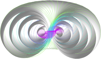
Figure 1. Hopf fibration via Villarceau circles on a hyperbolic family of torus surfaces.

The same motion was re-discovered independently by three of the authors of the present paper during the preparation of [li23] when it attracted our attention because of curious factorization properties. It can be parametrized by a quadratic polynomial with coefficients in the conformal geometric algebra ($\mathrm{CGA}$) that allows for a two-parametric set of factorizations with linear factors. This high number combined with its low algebraic degree distinguishes the conformal Villarceau motion from all other examples of rational motions with only one exception: The fairly simple planar rigid body motion that translates the moving object along a circle.

The purpose of this paper is to study and compare algebraic and geometric properties of factorizations of circular translation and conformal Villarceau motion. It will turn out that there are some similarities but also important differences. Ultimately, the conformal Villarceau motion sticks out as a prime example of a simple yet non-trivial rational motion with an outstanding number of fascinating geometric, algebraic, and kinematic properties.

This paper continues with a concise introduction to conformal geometric algebra, factorization theory of spinor polynomials over this algebra, and a kinematic map for conformal geometry in Section 2. We then proceed with a study of the factorizations of the circular translation and geometric interpretations in Section 3 before passing on to the conformal Villarceau motion in Section 4. We recall Dorst’s original definition, compute all of its factorizations, and discuss them in terms of the Euclidean geometry of the individual factors, in kinematic terms and also as conic section in the projective image space of conformal kinematics.

2. Preliminaries

This section intends to give a concise introduction to concepts used in the remainder of this article. For more detailed explanations we refer the reader to the references mentioned in the text.

Rigid body transformations are generated by an even number of reflections in planes. Similarly, conformal transformations in space can be defined as compositions of an even number of reflections (inversions) in spheres or planes (which usually are considered as “spheres” through the infinity point $\infty$). The non-linear nature of these transformations suggests that matrices may not always be the optimal tool to describe them. Moreover, the factorization theory of rational motions is not naturally formulated in matrix algebras. Hence we use the framework of conformal geometric algebra ($\mathrm{CGA}$). Here we will only be regarding the three-dimensional case.

2.1. Conformal Geometric Algebra

To construct $\mathrm{CGA}$ we first choose an orthonormal basis $\{e_{1},e_{2},e_{3},e_{+},e_{-}\}\in\mathbb{R}^{4,1}$ fulfilling the following conditions

$$e_{1}^{2}=e_{2}^{2}=e_{3}^{2}=e_{+}^{2}=1,\ e_{-}^{2}=-1.$$

The multiplication on this algebra is defined to be anticommutative:

$$e_{i}e_{j}=-e_{j}e_{i}\coloneqq e_{ij}\qquad\text{for}\quad i\neq j;\ i,j\in\{1,2,3,+,-\}$$

By linear extension this generates a real algebra, which is called the conformal geometric algebra.

On the $\mathrm{CGA}$ we define an involution called reversion, defined by inverting the order of multiplication of the basis elements. Using the anticommutativity of the multiplication we can write the reversion in the following way.

$$\tilde{e}_{i_{1},\ldots,i_{n}}=e_{i_{n},\ldots,i_{1}}=(-1)^{\tfrac{n(n-1)}{2}}e_{i_{1},\ldots,i_{n}}$$

A general element of $\mathrm{CGA}$ and it’s reverse can be written as

$$a=\sum_{l\subseteq\{1,2,3,+,-\}}a_{l}e_{l},\quad\tilde{a}=\sum_{l\subseteq\{1,2,3,+,-\}}a_{l}\tilde{e}_{l}$$

The cardinality of $l$ is called the grade of the element. This is defined for the basis vectors $e_{l}$ and for elements consisting only of elements of the same grade. Otherwise we say an element has mixed grade.

The basic objects we can represent in $\mathrm{CGA}$ are spheres, planes and points. Spheres with center $c$ and radius $r$ are represented by

(1) $$s=c_{x}e_{1}+c_{y}e_{2}+c_{z}e_{3}+\tfrac{1}{2}(1+c_{x}^{2}+c_{y}^{2}+c_{z}^{2}-r^{2})(e_{+}+e_{-})-e_{+}.$$

Note that $s\tilde{s}=\tilde{s}s=r^{2}$ is real. Points can be represented as spheres with zero radius. Planes can be seen as a limiting case of a sphere with radius approaching infinity. Hence the representation of planes looks slightly different. A plane with unit normal vector $n$ and oriented distance from the origin $d$ is given by

(2) $$p=n_{x}e_{1}+n_{y}e_{2}+n_{z}e_{3}+d(e_{+}+e_{-}).$$

Throughout this text, we will be using homogeneous coordinates for spheres, points, and planes. That is, spheres, points, and planes are also represented by non-zero scalar multiples of (1) or (2).

To be able to study kinematics in $\mathrm{CGA}$ we first have to define how an element can be acted upon. Any element $a$ of $\mathrm{CGA}$ (a sphere, point or plane) can be transformed by any other element $b$ via the sandwich product given by $a\mapsto ba\tilde{b}$. If $b$ is a sphere or a plane the action of $b$ describes a reflection in $b$. Through this we can construct the group of conformal displacements, as it is generated by reflection in spheres and planes. We denote the even sub-algebra of $\mathrm{CGA}$ as $\mathrm{CGA}_{+}$. It contains all linear combinations of elements of CGA with even grade and contains the compositions of an even number of reflections.

Acting with points on other objects is possible. It yields non-invertible maps which, nonetheless, are of high relevance in kinematics and factorization theory.

2.2. Spinor Polynomials and Their Factorization

Consider now a polynomial $C=\sum_{i=0}^{n}c_{i}t^{i}$ in the indeterminate $t$ and with coefficients $c_{i}\in\mathrm{CGA}_{+}$. Multiplication of polynomials is defined by the convention that the indeterminate $t$ commutes with all coefficients. Right evaluation of $C$ at $h\in\mathrm{CGA}_{+}$ is defined as

$$C(h)=\sum_{i=0}^{n}c_{i}h^{i}.$$

Because of non-commutativity, this is different from left evaluation $\sum_{i=0}^{n}h^{i}c_{i}$ (which we will not need in this text).

Denote by $\tilde{C}$ the polynomial obtained by conjugating its coefficient $c_{0}$, $c_{1}$, …, $c_{n}$. For $C$ to describe a conformal motion, it is necessary that $C\tilde{C}=\tilde{C}C$ is a non-zero real polynomial. If this condition is met and $C$ is of positive degree, we call $C$ a spinor polynomial [li23]. The action of spheres/points/planes is extended to the action of $C$ on spheres/points/planes via the formula

$$x\mapsto Cx\tilde{C}.$$

If $x$ is a point, then the right-hand side is a polynomial curve in homogeneous coordinates, that is, a rational curve in Cartesian coordinates. Hence one speaks of a rational conformal motion. Any factorization $C=PQ$ of $C$ with spinor polynomials $P$ and $Q$ corresponds to the decomposition of the motion into simpler sub-motions.

Most important for applications like in kinematics [hegedus13, gallet16] but also in discrete differential geometry [hoffmann24] are factorizations with linear spinor polynomial factors. We only consider factorizations of this type but, for the sake of brevity, only speak of “factorizations”. A lot is already known about such factorizations [li18, li23]:

• For generic $C$ of degree $n$ there exist finitely many factorizations. The total number depends on the number of real zeros of the polynomial $C\tilde{C}\in\mathbb{R}[t]$ and ranges between $n!$ for no real zeros of $C\tilde{C}$ and $(2n)!/(2^{n})$ for the maximum of $2n$ real zeros of $C\tilde{C}$.

• There are examples of spinor polynomials that do not admit any factorization.

• There are examples of spinor polynomials that admit infinitely many factorizations.

• The linear polynomial $t-h$ is a right factor of $C$ if and only if $h$ is a right zero of $C$. In other words, $C=C\textquoteright(t-h)$ for some spinor polynomial $C\textquoteright$, if and only if $C(h)=0$.

The last item shows that linear right factors and right zeros are closely related.

Examples of spinor polynomials with no or with infinitely many factorizations are rare. The only two known examples (up to conformal equivalence) of quadratic spinor polynomials with a two-parametric set of factorizations will be studied in this article.

2.3. A Map of Conformal Kinematics

The composition of an even number of reflections in spheres or planes is given by an algebra element $x\in\mathrm{CGA}_{+}$ of real norm, i.e., $x\tilde{x}=\tilde{x}x\in\mathbb{R}$. Since it is only unique up to non-zero scalar multiples, it is naturally viewed as a point of projective space $\mathbb{P}(\mathrm{CGA}_{+})=\mathbb{P}^{15}(\mathbb{R})$. In this way, we obtain a kinematic map from the group of conformal transformations into $\mathbb{P}^{15}(\mathbb{R})$.

Compositions from the left or from the right with fixed conformal transformations generate a transformation group of $\mathbb{P}^{15}(\mathbb{R})$ and thus determines a geometry of that space. Geometrically relevant entities in this context are:

• The Study variety $\mathcal{S}$, a projective variety of dimension ten and degree twelve that is given by the quadratic equations that encode the conditions $x\tilde{x}=\tilde{x}x\in\mathbb{R}$.

• The null quadric $\mathcal{N}$, given by vanishing condition of the real part of $x\tilde{x}$ (which equals the real part of $\tilde{x}x$).

Points in the intersection of $\mathcal{S}$ and $\mathcal{N}$ can be thought of as “singular” conformal displacements. While they do not describe proper conformal transformations, they are of geometric relevance. They arise quite naturally in conformal kinematics, for example as conformal scalings (see below) where the scale factor in the limit goes to zero.

Linear spinor polynomials $at+b$ describe particularly simple rational conformal motions [dorst16]. Depending on the sign of $h\tilde{h}$ with $h=a^{-1}b$, these elementary motions are classified as follows:

Conformal rotation ($h\tilde{h}>0$)::

A Euclidean rotation around a fixed axis and with variable angle or any conformal image thereof.

Conformal translation (transversion; $h\tilde{h}=0$)::

A Euclidean translation with fixed direction and variable distance or any conformal image thereof.

Conformal scaling ($h\tilde{h}<0$)::

A uniform scaling from a fixed center but with variable scaling factor or any conformal image thereof.

These elementary motions are illustrated in Figure 2. We display, in the top row, a typical surface generated by the points of a circle undergoing a Euclidean rotation, translation, or scaling. In the bottom row, the trajectory surface (a cyclide of Dupin) of a conformally equivalent motion is displayed. The arrows indicate point paths.

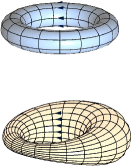
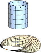
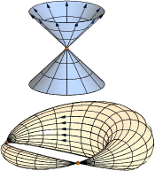
Figure 2. Elementary conformal motions: conformal rotation, translation (transversion), and scaling

3. The Circular Translation

In this section we consider a spinor polynomial in the sub-algebra $\langle 1,\mathbf{i},\mathbf{j},\mathbf{k},\varepsilon\rangle$, where

$$\mathbf{i}=-e_{2,3},\quad\mathbf{j}=e_{1,3},\quad\mathbf{k}=-e_{1,2},\quad\varepsilon=e_{1,2,3,+}+e_{1,2,3,-}.$$

The generating elements satisfy $\mathbf{i}^{2}=\mathbf{j}^{2}=\mathbf{k}^{2}=\mathbf{i}\mathbf{j}\mathbf{k}=-1$, $\varepsilon^{2}=0$ and $\mathbf{i}\varepsilon=\varepsilon\mathbf{i}$, $\mathbf{j}\varepsilon=\varepsilon\mathbf{j}$, $\mathbf{k}\varepsilon=\varepsilon\mathbf{k}$, whence it is the algebra of dual quaternions which we denote as $\mathbb{D}\mathbb{H}$. The polynomial we scrutinize is

$$C=t^{2}+1-\varepsilon(\mathbf{j}t+\mathbf{i}).$$

Observe that

$$C\tilde{C}=\tilde{C}C=M^{2}$$

where $M=t^{2}+1$. Hence, $C$ is indeed a spinor polynomial. Since it is defined over $\mathbb{D}\mathbb{H}$, it is even a motion polynomial in the sense of [hegedus13] and it describes a rigid body motion.

In order to write $C$ as product of two linear spinor polynomial factors, we use a general factorization algorithm [kalkan22, li23]. We use polynomial division to write $C=QM+R$ where $\deg R<\deg M=2$. (We will not make use of the fact that $Q=1$.) A linear right factor $H_{2}=t-h_{2}$ of $C$ is necessarily a right factor of $M$ and hence also of the linear remainder polynomial $R=r_{1}t+r_{0}$. Moreover, it should satisfy the spinor polynomial conditions $H_{2}\tilde{H}_{2}$, $\tilde{H}_{2}{H_{2}}\in\mathbb{R}[t]$ which boil down to $h_{2}\tilde{h}_{2}$, $\tilde{h}_{2}h_{2}$, $h_{2}+\tilde{h}_{2}\in\mathbb{R}$, c.f. [kalkan22]. For general spinor polynomials, these conditions are satisfied precisely by $h_{2}=-r_{1}^{-1}r_{0}$. However, in our case, we have $r_{1}=-\varepsilon\mathbf{j}$ which is not invertible. Existence of a right factor thus hinges on the existence of $h_{2}\in\mathbb{D}\mathbb{H}$ subject to the conditions:

(3) $$r_{1}h_{2}+r_{0}=0 t-h_{2} R$$    ( is right zero of )

$$h_{2}^{2}+1=0 h_{2} M$$    ( is a zero of )

$$h_{2}\tilde{h}_{2},\tilde{h}_{2}h_{2},h_{2}+\tilde{h}_{2}\in\mathbb{R} t-h_{2}$$    ( is a spinor polynomial)

Using the 16 yet unknown coefficients of $h_{2}$ as variables, we can convert these into a system of 39 algebraic equations. Among them, 13 are of degree one and 26 are of degree two. This system of equations allows for a straightforward solution. It turns out that all factorizations are over the dual quaternions $\mathbb{D}\mathbb{H}$:

(4) $$C=(t-\mathbf{k}-\varepsilon((1-\mu)\mathbf{j}-\lambda\mathbf{i}))(t+\mathbf{k}-\varepsilon(\lambda\mathbf{i}+\mu\mathbf{j})),\quad(\lambda,\mu)\in\mathbb{R}^{2}.$$

Remark 1.

The factorizations (4) of the motion polynomial $C$ are well-known [gallet16]. We have gained the additional insight that there are not more factorizations over $\mathrm{CGA}_{+}$ than there are over $\mathbb{D}\mathbb{H}$.

Several geometric interpretations of (4) are conceivable. To begin with, we may view the factors as parametric surfaces

$$h_{1}(\lambda,\mu)=\mathbf{k}-\lambda\varepsilon\mathbf{i}+(1-\mu)\varepsilon\mathbf{j},\quad h_{2}(\lambda,\mu)=-\mathbf{k}+\lambda\varepsilon\mathbf{i}+\mu\varepsilon\mathbf{j}$$

in the affine spaces parallel to the vectors $\varepsilon\mathbf{i}$ and $\varepsilon\mathbf{j}$ and through $\mathbf{k}$ and $-\mathbf{k}$, respectively. We see that the map $h_{2}(\lambda,\mu)\mapsto h_{1}(\lambda,\mu)$ is the composition of the reflection in the point $-\mathbf{k}$ followed by the translation by the vector $\varepsilon\mathbf{j}+2\mathbf{k}$.

A second interpretation of (4) is in terms of kinematics of the underlying motion. Each factor describes a rotation around an axis parallel to $\mathbf{k}$. Thus, $C$ parametrizes a planar rigid body motion. The respective rotation centers $c_{1}(\lambda,\mu)$, $c_{2}(\lambda,\mu)$ of $t-h_{1}$ and $t-h_{2}$ are the points

$$c_{1}(\lambda,\mu)=(1-\mu,\lambda)^{\intercal},\quad c_{2}(\lambda,\mu)=(-\mu,\lambda)^{\intercal}.$$

The point $c_{2}(\lambda,\mu)$ actually rotates around $c_{1}(\lambda,\mu)$. Its trajectory is a circle parametrized as

$$c_{2}(\lambda,\mu,t)=\frac{1}{1+t^{2}}(-\mu(1+t^{2})+2,\lambda(1+t^{2})+2t)^{\intercal}.$$

Denote by $\operatorname{dist}(a,b)$ the distance between two points $a$ and $b$. It is straightforward to deduce the following statements:

• For any $(\lambda,\mu)\in\mathbb{R}^{2}$ we have $\operatorname{dist}(c_{1}(\lambda,\mu),c_{2}(\lambda,\mu,t))=1$.

• For any two $(\lambda_{1},\mu_{1})$, $(\lambda_{2},\mu_{2})\in\mathbb{R}^{2}$ we have $\operatorname{dist}^{2}(c_{1}(\lambda_{1},\mu_{1}),c_{1}(\lambda_{2},\mu_{2}))=\operatorname{dist}^{2}(c_{2}(\lambda_{1},\mu_{1},t),c_{2}(\lambda_{2},\mu_{2},t))=(\lambda_{1}-\lambda_{2})^{2}+(\mu_{1}-\mu_{2})^{2}$.

We infer that $C$ describes the coupler motion of a parallelogram linkage where input and output crank are both of length $1$ (Figure 3). Each factorization of $C$ gives rise to one additional leg of length $1$. The coupler motion itself is the translation along a circle.

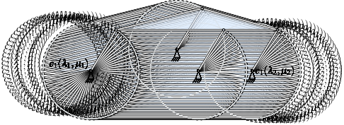
Figure 3. Circular translation and parallelogram linkage

For generic cases, a geometric relation between factorizations of spinor polynomials and the geometry in the kinematic image space space $\mathbb{P}^{15}(\mathbb{R})$ is well-understood. The interpretation of non-generic spinor polynomials is less clear. In the example of a circular translation, we can restrict ourselves to the projective space $\mathbb{P}^{3}(\mathbb{R})$ over the vector space and sub-algebra generated by $1$, $\varepsilon\mathbf{i}$, $\varepsilon\mathbf{j}$, and $\mathbf{k}$. We confine ourselves to observing that the rational curve parametrized by $C$ is, indeed, rather special.

The transformation group generated by left and right multiplications (coordinate changes in fixed and moving frame) turns $\mathbb{P}^{3}$ into a quasi elliptic space [klawitter15, Section 3.2.2]. Using homogeneous coordinates $x=x_{0}+x_{1}\varepsilon\mathbf{i}+x_{2}\varepsilon\mathbf{j}+x_{3}\mathbf{k}$, its invariant figure consists of the two planes with equations

$$\omega\colon x_{0}+\mathrm{i}x_{3}=0,\quad\overline{\omega}\colon x_{0}-\mathrm{i}x_{3}=0$$

(the intersection of the image space of planar kinematics with the null quadric $\mathcal{N}$) and the two points $[n_{1}]$, $[n_{2}]$ where

$$n_{1}=\varepsilon\mathbf{i}+\mathrm{i}\varepsilon\mathbf{j},\quad n_{2}=\varepsilon\mathbf{i}-\mathrm{i}\varepsilon\mathbf{j}$$

(c.f. [bottema90, Chapter 11, §2]).

The polynomial $C$ of (4) parametrizes a rational quadratic curve (a conic section) in this quasi elliptic space. It lies in the plane $x_{3}=0$ of pure translations. Moreover, $C(\mathrm{i})=n_{1}$ and $C(-\mathrm{i})=n_{2}$ so that the conic section contains the absolute points of quasi elliptic space. We may hence address it as a quasi elliptic circle.

4. The Conformal Villarceau Motion

The conformal Villarceau motion was introduced by L. Dorst in [dorst19]. In contrast to the circular translation of the previous section, it is not a rigid-body motion. Some of its curious geometric properties have been briefly covered in Section 1

We recall the parametric equation of the Villarceau motion of Dorst in [dorst19]. With

$$B_{-}\coloneqq e_{12}\quad\text{and}\quad B_{+}\coloneqq e_{3+}$$

it is given by

$$C=\exp(-B_{-}\tfrac{\varphi}{2})\exp(-B_{+}\tfrac{\varphi}{2}).$$

Expanding this in a Taylor series, simplifying using, Using $B_{-}^{2}=B_{+}^{2}=-1$, and separating even and odd parts, this can be written as

$$C=(\cos\varphi+B_{-}\sin\varphi)(\cos\varphi+B_{+}\sin\varphi).$$

Substituting $t=-\cot{\varphi}$ we arrive at the polynomial

$$C=(t-B_{-})(t-B_{+})=t^{2}-t(e_{12}+e_{3+})+e_{123+}.$$

It admits one factorization with linear spinor polynomial factors by construction. We wish to find all of these factorizations. In doing so, we follow the general procedure that has already been outlined in Section 3. Once more, the norm polynomial is

$$C\tilde{C}=\tilde{C}C=M^{2}$$

where $M=(t^{2}+1)^{2}$. Using polynomial division we write $C=QM+R$ where $R=r_{1}t+r_{0}$ and

$$r_{1}=-e_{12}-e_{3+},\quad r_{0}=e_{123+}-1.$$

Again, $r_{1}$ is not invertible so that we have to solve the system of equations (3). Using the 16 yet unknown coefficients of $h_{2}$ as variables, we can convert these into a system of 43 algebraic equations. Among them, 17 are of degree one and 26 are of degree two. Solving the 17 linear equations results in

(5) $$h_{2}=e_{12}+s_{x}x+s_{y}y+s_{z}z$$

where

(6) $$s_{x}=2(e_{1+}-e_{23}),\quad s_{y}=2(e_{2+}+e_{13}),\quad s_{z}=2(e_{3+}-e_{12}),$$

(7) $$\text{and}\quad x^{2}+y^{2}+(z-\tfrac{1}{4})^{2}-\tfrac{1}{16}=0.$$

Since the vectors $e_{1+}-e_{23}$, $e_{2+}+e_{13}$, $e_{3+}-e_{12}$ are pairwise perpendicular and of equal length we may say that $h_{2}$ lies on a sphere given by (5)–(7). If $S(u,v)$ is some parametrization of this sphere, we have

(8) $$h_{2}(u,v)=m+\tfrac{1}{4}S(u,v)$$

where $m=\tfrac{1}{2}(e_{12}+e_{3+})$. Using polynomial division, we find $C=(t-h_{1}(u,v))(t-h_{2}(u,v))$ where

(9) $$h_{1}(u,v)=m-\tfrac{1}{4}S(u,v).$$

Thus, we can say: The factors $t-h_{1}(u,v)$ and $t-h_{2}(u,v)$ in the factorizations of the Villarceau motion are parameterized by the points of a sphere. The map $h_{1}(u,v)\mapsto h_{2}(u,v)$ is the reflection in the sphere center $m$. This implies commutativity of $h_{1}(u,v)$ and $h_{2}(u,v)$ which can, of course, also be confirmed by a straightforward calculation.

Elementary conformal motions are more difficult to grasp intuitively than mere rotations or translations. Hence, a kinematic explanation of the infinitely many factorizations of $C=(t-h_{1}(u,v))(t-h_{2}(u,v))$ is a challenging task. Lets first look at the individual elementary motions $H_{1}=s-h_{1}(u,v)$ and $H_{2}=t-h_{2}(u,v)$, parametrized by different parameters $s$ and $t$. In this sense, their product creates a two-parametric rational motion. It is readily confirmed that

(10) $$H_{1}H_{2}=H_{2}H_{1}.$$

For any point $x$, the trajectory surface $D_{x}=H_{1}H_{2}x\tilde{H}_{2}\tilde{H}_{1}$ is a cyclide of Dupin. This can be seen by

1. verifying that the parameter lines are circles and showing that

2. the second fundamental form of $D_{x}$ is diagonal.

This implies that the curvature lines of $D_{x}$ are circles which is a characteristic property of cyclides of Dupin.

The parameter line circles are point trajectories under the elementary motions given by $H_{1}$ and $H_{2}$, respectively. The trajectory of point $x$ under the one-parametric rational motion $C$ is obtained as diagonal surface curve for $s=t$. In a conformal transformation of $D_{x}$ to a torus, it is mapped to a Villarceau circle. Hence, we follow [dorst19] and address it as Villarceau circle on a Dupin cyclide. Different values of $u$ and $v$ provide different Dupin cyclides but the same Villarceau circle on them. This is illustrated in Figure 4.

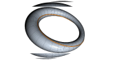
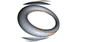
Figure 4. Different Dupin cyclides with the same Villarceau circle

The interpretation of the conformal Villarceau motion $C$ in kinematic image space is more involved than in case of the circular translation and we cannot hope to resolve all mysteries. The geometry of kinematic image space is not among the classical non-Euclidean geometries and a complete system of geometric invariants is not known. Therefore, we confine ourselves to highlight some peculiarities.

The polynomial $C$ parametrizes a rational curve of degree two in $\mathbb{P}^{15}(\mathbb{R})$. It intersects the null quadric $\mathcal{N}$ in only two points $[n_{1}]$, $[n_{2}]$ where

$$n_{1}=C(\mathrm{i})=e_{123+}-1-\mathrm{i}(e_{12}+e_{3+}),\quad n_{2}=C(-\mathrm{i})=e_{123+}-1+\mathrm{i}(e_{12}+e_{3+}).$$

It is known [scharler21] that factorizability is related the connecting lines of intersection points of $C$ and $\mathcal{N}$. In our case, these are the conic tangents in $[n_{1}]$ and $[n_{2}]$ as well as their connecting line. More precisely, the linear remainder polynomial $R$ in the expression $C=QM+R$ parametrizes one such line. We already observed that its leading coefficient $r_{1}$ is not invertible. A direct computation shows that none of the points on the connecting line of $[n_{1}]$ and $[n_{2}]$ or on the tangents of $C$ in $[n_{1}]$ and $[n_{2}]$ are invertible. This explains why conventional factorization attempts (with only finitely many factorizations) fail in case of $C$ and it emphasizes the importance of non-invertible elements of $\mathrm{CGA}_{+}$. Not much seems to be known about their geometry as points of $\mathbb{P}(\mathrm{CGA}_{+})$.

5. Conclusion

We have investigated the two known examples of quadratic spinor polynomials with a two parameteric set of factorizations. The underlying motions are the fairly simple translation along a circle and the Villarceau motion of [dorst19]. Both motions have curious algebraic and geometric properties and exhibit some similarities but also differences. Most notably, the factors of the Villarceau motion are parametrized by the points of a sphere and not a plane. They correspond in the reflection in the sphere center and do commute, c.f. (10). While the circular translation can be viewed as a quasi elliptic circle in kinematic image space, the analogous interpretation of the Villarceau motion is less obvious. For the circular translation the point on the secant connecting its null points are non-invertible, for the Villarceau motion this is the case along the secant but also along the tangents. The circular translation can be created mechanically by a parallelogram linkage with factorizations corresponding to possible cranks. For the factorizations of the conformal Villarceau motion and its trajectories we gave an interpretation in terms of Dupin cyclides that share a Villarceau circle.

A more systematic study of the conformal Villarceau motion is planned for the future. The question for low degree spinor polynomials with many factorizations apart from circular translation and conformal Villarceau motion remains wide open.