From Large to Small Datasets:
Size Generalization for Clustering Algorithm Selection

Abstract

In clustering algorithm selection, we are given a massive dataset and must efficiently select which clustering algorithm to use. We study this problem in a semi-supervised setting, with an unknown ground-truth clustering that we can only access through expensive oracle queries. Ideally, the clustering algorithm’s output will be structurally close to the ground truth. We approach this problem by introducing a notion of size generalization for clustering algorithm accuracy. We identify conditions under which we can (1) subsample the massive clustering instance, (2) evaluate a set of candidate algorithms on the smaller instance, and (3) guarantee that the algorithm with the best accuracy on the small instance will have the best accuracy on the original big instance. We provide theoretical size generalization guarantees for three classic clustering algorithms: single-linkage, $k$-means++, and (a smoothed variant of) Gonzalez’s $k$-centers heuristic. We validate our theoretical analysis with empirical results, observing that on real-world clustering instances, we can use a subsample of as little as 5% of the data to identify which algorithm is best on the full dataset.

1 Introduction

Clustering is a fundamental task with many applications, yet it is often unclear what mathematically characterizes a “good” clustering. As a result, researchers have proposed a wide variety of clustering algorithms, including hierarchical methods such as single- and complete-linkage, and center-based methods such as $k$-means++ and $k$-centers. The best algorithm for a given dataset varies, but there is little guidance on selecting a good algorithm. In practice, Ben-David [12] writes, clustering algorithm selection is often done “in a very ad hoc, if not completely random, manner,” which is regrettable “given the crucial effect of [algorithm selection] on the resulting clustering.”

We study algorithm selection in a semi-supervised setting where there is a ground truth clustering of a massive dataset that we can access through expensive ground-truth oracle queries, modeling interactions with a domain expert, for example. Semi-supervised clustering has been widely studied [43, 32, 18, 11, 9] and has many applications, such as image recognition [14] and medical diagnostics [23]. We summarize the goal of semi-supervised algorithm selection as follows.

Goal 1.1.

Given a set of candidate algorithms, select an algorithm that will best recover the ground truth. The algorithm selection procedure should have low runtime and use few ground-truth queries.

Clustering algorithm selection is at the heart of an important gap between clustering theory and practice [13, 41, 7, 12, 2]. In the clustering theory literature, one often implicitly assumes that the ground truth minimizes an objective function $h$ (such as $k$-means or -centers), and the literature provides algorithms to minimize $h$. However, identifying $h$ might be as hard as identifying the ground truth in the first place. Moreover, the ground truth need not align well with any previously studied objective. Even if the ground truth is known to align with some $h$, it may be ${\sf NP}$-hard to minimize $h$. In this case, one might aim to approximately minimize $h$. However, strong approximation guarantees with respect to $h$ do not immediately imply low error with respect to the ground truth (Definition 2.1 in Section 2), which is ultimately what many practitioners care about. Thus, theoretical approximation guarantees for clustering algorithms may not directly identify good clustering algorithms in practice.

Given a massive dataset $\mathcal{X}$, a natural—but computationally inefficient—approach to attack Goal 1.1 would be to (1) run the candidate algorithms on $\mathcal{X}$; (2) subsample $\mathcal{X}$; and (3) evaluate which algorithm’s output is closest to the ground truth by querying the ground-truth oracle on the subsample. This is easy to analyze statistically (approximation guarantees would follow from Hoeffding bounds), but the runtime is large. Therefore, we flip the order of operations and ask,

Question 1.2.

Given a huge clustering dataset, can we (1) subsample the dataset, (2) evaluate a set of candidate algorithms on the subsample, and (3) guarantee that the algorithm with the best accuracy on the subsample will have the best accuracy on the original massive instance?

We refer to property (3) as size generalization since we require that an algorithm’s accuracy can be estimated using a smaller instance. When size generalization holds, we can use the smaller dataset to rank the algorithms efficiently (both in terms of the number of samples and ground-truth queries).

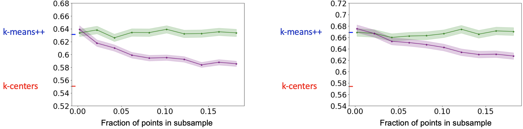
Figure 1: Illustration of size generalization. The $y$-axes plot the accuracy of $k$-means++ and a $k$-centers heuristic on two MNIST instances containing two 500-point clusters. The green and purple lines show accuracies of proxy versions of these algorithms on subsamples, with 95% confidence intervals over $10^{3}$ repetitions. Even a small subsample shows that $k$-means++ outperforms $k$-centers.

Figure 1 shows this approach applied to selecting between two algorithms. Surprisingly, sampling only 5% of the data is sufficient to identify the better algorithm. We show this method also works well for other datasets. The challenge lies in proving that Question 1.2 can be answered affirmatively. For example, for algorithms that are sensitive to outliers, such as $k$-means++, simply running the algorithm as is on the subsample can fail. Nonetheless, we identify conditions and algorithms under which size generalization is possible with respect to an arbitrary ground truth clustering.

1.1 Our contributions

We formalize the notion of size generalization for clustering algorithm accuracy, which aims to answer Question 1.2. This question applies beyond clustering to combinatorial algorithm selection more broadly, where the goal is to determine which of several candidate algorithms has the best performance on a set of large combinatorial problems using small versions of the problems. This is a common approach in empirical algorithm selection [e.g., 38, 26, 20, 30], but there is scant theoretical guidance. As a first step towards a general theory of size generalization, we answer Question 1.2 for single-linkage clustering, (a smoothed version of) Gonzalez’s $k$-centers heuristic, and the $k$-means++ algorithm.

$k$-centers:

First, we bound the number of samples $m$ sufficient to estimate the accuracy of a smoothed version of Gonzalez’s $k$-centers heuristic, which we call softmax $k$-centers. We provide approximation guarantees for softmax $k$-centers with respect to the $k$-centers objective and show empirically that it matches or—surprisingly—even outperforms Gonzalez’s algorithm both in terms of the $k$-centers objective as well as the ground truth accuracy on several real-world datasets. We provide a size generalization procedure that uses Markov Chain Monte Carlo (MCMC) to approximate the distribution over cluster centers induced by softmax $k$-centers. Our bound on $m$ depends on how close this distribution is to a uniform distribution. If the distribution places a large mass on a single point, we naturally need more samples from the dataset to simulate it. We show that under natural assumptions, our bound on the number of samples is sublinear in the size of the dataset.

$k$-means++:

Next, we bound the number of samples sufficient to estimate the accuracy of $k$-means++ (the one-step version analyzed by Arthur and Vassilvitskii [1]). As with $k$-centers, we use an MCMC procedure, and our bound depends on how far the distribution over cluster centers induced by the $k$-means++ algorithm is from uniform. We then appeal to results by [4] to show that this bound is sublinear in the size of the dataset under natural assumptions.

Single linkage:

Finally, we analyze the single-linkage algorithm, which is known to be unstable in theory, but our experiments (Section 5) illustrate that its performance can often be estimated on a subsample. To understand this unexpected phenomenon, we identify a necessary and sufficient condition under which size generalization is possible for single-linkage. In particular, we characterize when the trajectory of running single-linkage on the original instance $\mathcal{X}$ is similar to that of running the algorithm on a subsample. Our condition is based on a relative ratio between the inter-cluster and intra-cluster distances in the single linkage clustering of $\mathcal{X}$. If this ratio is small, the single linkage procedure is robust to subsampling. We show that the dependence on this ratio is also necessary: for clustering instances in which this ratio is large, single linkage’s performance may be sensitive to the deletion of even a single randomly selected point. We believe this analysis may be of independent interest, as it helps identify when this well-known algorithm is unstable.

Key challenges.

Clustering algorithms often have a combinatorial, sequential nature that is sensitive to the inclusion of individual data points (see Figures 2 and 4). Consequently, it is challenging to characterize an algorithm’s performance upon deleting points from the dataset. Moreover, we make no assumptions on the ground truth clustering (e.g., that it minimizes some objective), as these assumptions may be difficult to verify in practice. The ground truth clustering is arbitrary and could potentially be chosen adversarially (see Figure 5 of Appendix A.2).

1.2 Related work

Size generalization vs coresets.

Our work complements a line of research on coresets [e.g., 29, 19, 24]. Suppose $\mathcal{X}$ is a clustering instance, and the goal is to find $k$ centers that minimize a known objective $h$. A coreset is a subset $\mathcal{X}_{{\sf c}}\subset\mathcal{X}$ such that for any set $C$ of $k$ centers, $h(C;\mathcal{X})\approx h(C;\mathcal{X}_{{\sf c}})$. Coresets lead to efficient approximation algorithms for minimizing $h$. However, we aim to maximize accuracy with respect to a ground truth clustering, and coresets do not provide the desired guarantees. Even if the ground truth clustering corresponds to minimizing $h$, there is no guarantee that an approximation to the optimal solution of $h$ implies an approximation to the ground truth. This is the key distinction between our results and coresets: the ground truth is not assumed to minimize any known objective, and we aim to provide approximation guarantees directly with respect to the ground truth.

Additional related work.

Ashtiani and Ben-David [2] study a semi-supervised approach to learning a data representation for downstream clustering. In contrast, we study the problem of algorithm selection. Voevodski et al. [40] study how to recover a low-error clustering with respect to a ground-truth clustering using few distance queries. They assume the instance is “approximation stable” (a concept introduced by Balcan et al. [7]): any clustering that approximates the $k$-medians objective is close to the ground truth. In contrast, we make no assumptions on the relation of the ground truth to any clustering objective. We discuss additional related work in Appendix A.

Paper organization.

Section 2 states our notation and problem statement. Section 4 covers our results for single linkage. Section 3 covers our results for $k$-centers and $k$-Means++. Section 5 presents our empirical results. Discussion of additional related work, key challenges, and additional empirical results can be found in Appendix A. Omitted proofs can be found Appendix C.

2 Preliminaries

We use $\mathcal{X}\subset\mathbb{R}^{d}$ to denote a finite clustering instance and $\mathcal{P}(\mathcal{X})\stackrel{{\scriptstyle\textup{def}}}{{=}}\{S\subset\mathbb{R}^{d}:S\subset\mathcal{X}\}$. The collection $\{S_{1},...,S_{k}\}$ is a $k$-clustering of $\mathcal{X}$ if it partitions $\mathcal{X}$. We use $d:\mathcal{X}\times\mathcal{X}\to\mathbb{R}_{\geq 0}$ to denote an arbitrary metric over $\mathcal{X}$. We use $x\approx_{\epsilon}y$ for the relation $y-\epsilon\leq x\leq y+\epsilon$. We define $\Sigma_{n}$ to be the set of permutations of $[n]:=\{1,...,n\}$. For an event $E$, $\bar{E}$ denotes the complement of $E$, and $\mathds{1}{\left\{E\right\}}$ denotes the indicator of $E$. We measure error with respect to the ground truth as follows:

Definition 2.1 (e.g., Ashtiani and Ben-David [2]).

Let $\mathcal{X}=\{x_{i}\}_{i=1}^{n}$ be a clustering instance, $\mathcal{C}=(C_{1},...,C_{k})$ be a $k$-clustering of $\mathcal{S}\subset\mathcal{X}$, and $\mathcal{G}=(G_{1},...,G_{k})$ be a $k$-clustering of $\mathcal{X}$. We define the cost of clustering $\mathcal{C}$ with respect to the ground truth $\mathcal{G}$ as

$${\sf{cost}}_{\mathcal{G}}\left(\mathcal{C}\right)\stackrel{{\scriptstyle\textup{def}}}{{=}}\frac{1}{\left\lvert\mathcal{S}\right\rvert}\min_{\sigma\in\Sigma_{k}}\sum_{x\in\mathcal{S}}\sum_{j\in[k]}\mathds{1}{\left\{x\in C_{\sigma(j)}\,\land\,x\notin G_{j}\right\}}.$$

When convenient, we may also use the accuracy of a clustering $\mathcal{C}$ to refer to $1-{{\sf{cost}}_{\mathcal{G}}\left(\mathcal{C}\right)}$.

Distance computations and—in our semi-supervised model—ground truth queries are the key bottlenecks in clustering algorithm selection, so we evaluate our results in terms of the number of queries to a distance oracle and ground-truth oracle. A distance oracle takes in $u,v\in\mathcal{X}$ and outputs the distance $d(u,v)$. Given a target number of clusters $k$ and query $x\in\mathcal{X}$, the ground truth oracle returns an index $j\in[k]$ in constant time. The ground truth clustering is the partition $C_{1},\dots,C_{k}$ of $\mathcal{X}$ such that for all $x\in C_{j}$, the ground truth oracle returns the label $j$.

The ground-truth oracle can be implemented in several natural scenarios, for example, by querying a domain expert. This approach of incorporating a domain expert’s knowledge to obtain a good clustering is inspired by similar approaches in previous work [e.g., 39, 3, 37]. This setting arises in many real-world examples, such as in medical pathology [35], where it is expensive to cluster/classify the entire dataset, but obtaining cluster labels for a small subset of the data is feasible.

The ground-truth oracle can also be implemented using a same-cluster query oracle, which has been widely studied in prior work [e.g., 3, 37, and references therein]. Given a pair $x,y\in\mathcal{X}$, a same-cluster query oracle identifies whether $x,y$ belong to the same cluster under the ground truth. One can generate a ground-truth oracle response for all $x\in S\subset\mathcal{X}$ by making just $O(\left\lvert S\right\rvert k)$ queries to the same-cluster oracle.

3 $k$-Means++ and $k$-Centers Clustering

In this section, we provide size generalization bounds for $k$-means++ and $k$-centers clustering. Given $x\in\mathcal{X}$ and $C:=\{c_{1},...,c_{k}\}\subset\mathbb{R}^{d}$, let $d_{\sf center}(x;C)\stackrel{{\scriptstyle\textup{def}}}{{=}}\min_{c_{i}\in C}d(x,c_{i})$. The clustering of $\mathcal{X}$ induced by $C$ is the partition $S_{1},...,S_{k}$ where $S_{i}=\{x:{i=\operatorname*{argmin}}\left\lVert x-c_{j}\right\rVert\}$ (with fixed but arbitrary tie-breaking). The $k$-means problem minimizes the objective $\sum_{x\in\mathcal{X}}d_{\sf center}(x;C)^{2}$, for which $k$-means++ provides a multiplicative $\log k$-approximation [1]. The $k$-centers problem minimizes the objective function $\max_{x\in\mathcal{X}}d_{\sf center}(x;C)$, for which Gonzalez’s heuristic [1985] is a multiplicative 2-approximation.

Input: Instance $\mathcal{X}\subset\mathbb{R}^{d}$, $k\in{\mathbb{Z}}_{\geq 0}$, $f:\mathbb{R}\times\mathcal{P}(\mathcal{X})\to\mathbb{R}_{\geq 0}$

Set $C^{1}=\{c_{1}\}$ with $c_{1}\sim\text{Unif}(\mathcal{X})$

for $i=2,3,\dots,k$ do

       Select $c_{i}=y\in\mathcal{X}$ with probability proportional to $f(d_{\sf center}(y;C^{i-1});\mathcal{X})$

       Set $C^{i}=C^{i-1}\cup\{x\}$

      

end for

Return: $C^{k}$

Algorithm 1 ${\sf Seeding}(\mathcal{X},k,f$)

Both algorithms are instantiations of Algorithm 1, ${\sf Seeding}$. Under ${\sf Seeding}$, the first center is uniformly sampled. Given $i-1$ centers $C^{i-1}$, the $i^{th}$ center $c_{i}$ is sampled according to a function $f$, with probability $\propto f(d_{\sf center}(c_{i};C^{i-1});{\mathcal{X}})$. The algorithm returns after selecting $k$ centers and requires $O({|\mathcal{X}|}k)$ distance oracle queries. Under $k$-means++, $f(z;\mathcal{X})=z^{2}$ and under Gonzalez’s heuristic, $f(z;\mathcal{X})=\mathds{1}{\left\{z=\max_{x\in\mathcal{X}}d_{\sf center}(x;C^{i-1})\right\}}$.

Input: Instance $\mathcal{X}=(x_{1},...,x_{mk})\subset\mathbb{R}^{d}$, $k,m\in{\mathbb{Z}}_{\geq 0}$, $f:\mathbb{R}\times\mathcal{P}(\mathcal{X})\to\mathbb{R}_{\geq 0}$

Set $C^{1}=\{c_{1}\}$ with $c_{1}\sim\text{Unif}(\mathcal{X})$

$\ell=1$

for $i=2,3,\dots,k$ do

       Set $x=x_{\ell}$, $d_{x}=d_{\sf center}(x;C^{i-1})$, $\ell=\ell+1$

       for $j=2,3,\dots,m$ do

             Set $y=x_{\ell}$, $d_{y}=d_{\sf center}(y;C^{i-1})$, $\ell=\ell+1$

             if $f(d_{y};\mathcal{X})/f(d_{x};\mathcal{X})>{\sf{U}(0,1)}$ then

                   Set $x=y$ and $d_{x}=d_{y}$

                  

             end if

            

       end for

      Set $C^{i}=C^{i-1}\cup\{x\}$

      

end for

Return: $C^{k}$

Algorithm 2 ${\sf ApxSeeding}(\mathcal{X},k,m,f)$

To efficiently estimate ${\sf Seeding}$’s accuracy with a subsample, we use an MCMC approach, ${\sf ApxSeeding}$. In Sections 3.1 and 3.2, we apply ${\sf ApxSeeding}$ to $k$-centers and $k$-means clustering. ${\sf ApxSeeding}$ (Algorithm 2) runs an $m$-step Metropolis-Hastings procedure to select centers, requiring only $O(mk^{2})$ distance oracle queries. Acceptance probabilities are controlled by $f$. ${\sf ApxSeeding}$ generalizes an approach by Bachem et al. [4], who use MCMC to obtain a sublinear-time $k$-means approximation. However, we aim to estimate the clustering algorithms’ accuracies. Thus, we generalize their framework to work with general functions $f$ and give accuracy guarantees.

Theorem 3.1 specifies the choice of $m$ in ${\sf ApxSeeding}$ that guarantees an $\epsilon$-approximation to the accuracy of ${\sf Seeding}$. Our bound depends linearly on $\zeta_{k,f}(\mathcal{X})$, a parameter measuring the smoothness of the distribution over centers induced by sampling according to $f$ in ${\sf Seeding}$ (line 1). Ideally, if this distribution induced by $f$ is close to uniform, then $\zeta_{k,f}(\mathcal{X})$ is close to 1, but if it is very biased towards selecting certain points, then $\zeta_{k,f}(\mathcal{X})$ may be as large as $n$.

Theorem 3.1.

Let $\mathcal{X}\subset\mathbb{R}^{d}$, $\epsilon,\epsilon^{\prime}>0,\delta\in(0,1)$, and $k\in{\mathbb{Z}}_{>0}$. Define

$$\zeta_{k,f}(\mathcal{X})\stackrel{{\scriptstyle\textup{def}}}{{=}}\max_{Q\subset\mathcal{X}:\left\lvert Q\right\rvert\leq k}\max_{x\in\mathcal{X}}\frac{nf(d_{\sf center}(x;Q);\mathcal{X})}{\sum_{y\in\mathcal{X}}f(d_{\sf center}(y;Q);\mathcal{X})}$$

and $m=O({\zeta_{k,f}}(\mathcal{X})\log(k/\epsilon))$. Let $S$ be the partition of $\mathcal{X}$ induced by ${\sf Seeding}{(\mathcal{X},k,f)}$ and $S^{\prime}$ be the partition of $\mathcal{X}$ induced by ${\sf ApxSeeding}(\mathcal{X}_{mk},k,m,f)$ where $\mathcal{X}_{mk}$ is a random sample of $mk$ points from $\mathcal{X}$ drawn with replacement. For any ground truth partition $\mathcal{G}$ of $\mathcal{X}$, we have $\operatorname*{\mathbb{E}}\left[{\sf{cost}}_{\mathcal{G}}\left(S^{\prime}\right)\right]\approx_{\epsilon}\operatorname*{\mathbb{E}}\left[{\sf{cost}}_{\mathcal{G}}\left(S\right)\right]$. Moreover, given $S^{\prime}$, one can compute an estimate $\hat{c}_{\mathcal{G}}(S^{\prime})$ such that $\hat{c}_{\mathcal{G}}(S^{\prime})\approx_{{\epsilon^{\prime}}}{\sf{cost}}_{\mathcal{G}}\left(S^{\prime}\right)$ with probability $1-\delta$ using ${O}(k{{\epsilon^{\prime}}}^{-2}\log(\delta^{-1}))$ ground-truth queries.

Proof sketch.

Let $p^{\prime}(T)$ and $p(T)$ be the probability of outputing $T$ from ${\sf ApxSeeding}(\mathcal{X}_{mk},k,m,f)$ and ${\sf Seeding}(\mathcal{X},k,f)$ respectively. Let $p(c_{i}|C^{i-1})$ and $p^{\prime}(c_{i}|C^{i-1})$ be the probability of sampling $c_{i}$ as the $i$-th center, given $C^{i-1}$ was selected up to the $(i-1)$-th step in ${\sf Seeding}{(\mathcal{X},k,f)}$ and ${\sf ApxSeeding}{(\mathcal{X}_{mk},k,m,f)}$, respectively. We use MCMC convergence rates [15] to show that when $m=O(\zeta_{k,f}(\mathcal{X})\log(k/\epsilon))$, these conditional distributions are close in total variation distance, and hence, the total variation distance between $p$ and $p^{\prime}$ is at most $\epsilon.$ This implies the first statement. The second statement follows from a union and Hoeffding bound. ∎

In Section 3.1, we apply Theorem 3.1 to the $k$-centers problem. For $k$-means++, Bachem et al. [4] provide sufficient conditions to ensure $\zeta_{k,f}(\mathcal{X})$ is small, as we discuss in Section 3.2.

3.1 Application to $k$-Centers Clustering

We now apply our MCMC framework to approximate the accuracy of Gonzalez’s heuristic. However, there is an obstacle to a direct application: at each step of Gonzalez’s heuristic, the point with the maximum distance from its center is selected with probability 1, so $\zeta_{k,f}(\mathcal{X})=n$. Instead, we analyze a smoothed version of Gonzalez’s algorithm, which we define as

$${\sf SoftmaxCenters}(\mathcal{X},k,\beta)\stackrel{{\scriptstyle\textup{def}}}{{=}}{\sf Seeding}(\mathcal{X},k,f_{{\sf SoftmaxCenters}}),$$

where $f_{{\sf SoftmaxCenters}}(z;\mathcal{X})\stackrel{{\scriptstyle\textup{def}}}{{=}}\exp(\beta z)$. Theorem 3.2 shows that ${\sf SoftmaxCenters}$ provides a constant-factor approximation to the $k$-centers objective on instances with well-balanced $k$-centers solutions  [31, 22, 5]: given $\mu_{\ell},\mu_{u}\in(0,1)$, we say a clustering instance $\mathcal{X}$ is ($\mu_{\ell},\mu_{u}$)-well-balanced with respect to a partition $S_{1},\dots,S_{k}$ if for all $i\in[k]$, $\mu_{\ell}|\mathcal{X}|\leq|{S}_{i}|\leq\mu_{u}|\mathcal{X}|$.

Theorem 3.2.

Let $\mathcal{X}\subset\mathbb{R}^{d}$, $k\in{\mathbb{Z}}_{\geq 0}$, $\gamma>0$ and $\delta\in(0,1)$. Let $S_{{\sf OPT}}$ be the partition of $\mathcal{X}$ induced by the optimal $k$-centers solution $C_{{\sf OPT}}$, and suppose $\mathcal{X}$ is $(\mu_{\ell},\mu_{u})$-well-balanced with respect to $S_{{\sf OPT}}$. Let $C={\sf SoftmaxCenters}\left(\mathcal{X},k,\gamma^{-1}\log\left(k^{2}\mu_{u}\mu_{\ell}^{-1}\delta^{-1}\right)\right).$ With probability $1-\delta$, $\max_{x\in\mathcal{X}}d_{\sf center}(x;C)\leq 4\max_{x\in\mathcal{X}}d_{\sf center}(x;C_{{\sf OPT}})+\gamma$.

Proof sketch.

Let $S_{{\sf OPT}}=\{S_{1},...,S_{k}\}$ and let ${\sf OPT}$ denote the optimal $k$-centers objective value. Let $S_{\sigma(i)}\in S_{{\sf OPT}}$ be such that $c_{i}\in S_{\sigma(i)}$, and let ${C^{i-1}}\subset C$ denote the centers chosen in the first $i-1$ iterations of ${\sf SoftmaxCenters}$. The idea is to show that for any $i\in\{2,...,k-1\}$, either $m_{i}\stackrel{{\scriptstyle\textup{def}}}{{=}}\max_{x\in\mathcal{X}}d(x;{C^{i-1}})\leq 4{\sf OPT}+\gamma$, or else with good probability, $c_{i}$ belongs to a different partition $S_{\sigma(i)}$ than any of $c_{1},...,c_{i-1}$ (i.e., $\sigma(i)\neq\sigma(j)$ for any $j<i$). Indeed, if $m_{i}>4{\sf OPT}+\gamma$, then let $B\stackrel{{\scriptstyle\textup{def}}}{{=}}\{x:x\in S_{\sigma(j)}\text{ for some }j<i\}$ and $\ell\in[k]$ be the index of the optimal cluster in which $\exists y\in S_{\ell}$ with $d(y;C^{i-1})=m_{i}>4{\sf OPT}+\gamma$. By triangle inequality and well-balancedness, we are able to bound $\operatorname*{\mathbb{P}}\left\{c_{i}\in B\right\}\leq\delta/k$, and the statement follows by union bounding over $i=2,...,k$. ∎

Surprisingly, our empirical results (Section 5) show that for several datasets, ${\sf SoftmaxCenters}$ achieves a lower objective value than Gonzalez’s heuristic, even for $\beta=O(1)$. Intuitively, this is because Gonzalez’s heuristic is pessimistic: it assumes that at each step, the best way to reduce the objective value is to put a center at the farthest point. In practice, a smoother heuristic may yield a lower objective value (a phenomenon also observed by García-Díaz et al. [25]).

Theorem 3.3 shows that for datasets bounded by a sphere of radius $R$, the $\zeta_{k,f}$ term in Theorem 3.1 can be bounded only in terms of $\beta$ and $R$.

Theorem 3.3.

If $\max_{x,y\in\mathcal{X}}d(x,y)\leq R$, then $\zeta_{k,{\sf SoftmaxCenters}}(\mathcal{X})\leq\exp(2\beta R)$.

Proof.

For any $Q$, let $x_{Q}^{\star}=\operatorname*{argmax}_{x\in\mathcal{X}}\exp(\beta d_{\sf center}(x;Q))$. Then, $\sum_{y\not=x^{\star}_{Q}}\exp(\beta d_{\sf center}({y};Q))+\exp(\beta d_{\sf center}(x_{Q}^{\star};Q))\geq(n-1)+\exp(\beta d_{\sf center}(x_{Q}^{*},Q))$. Meanwhile, $\exp(\beta d_{\sf center}(x_{Q}^{*},Q))\leq\exp(2\beta R)$. Since $h(x)=\frac{x}{(n-1)+x}$ and $g(x)=\frac{xa}{(x-1)+a}$ are increasing in $x$ for $a>1$, we conclude that

$$\zeta_{k,{\sf SoftmaxCenters}}(\mathcal{X})\stackrel{{\scriptstyle\textup{def}}}{{=}}n\cdot\max_{Q\subset\mathcal{X}:|Q|\leq k}\max_{x\in\mathcal{X}}\frac{\exp(\beta d_{\sf center}(x;Q))}{\sum_{y\in Q}\exp(\beta d_{\sf center}(y;Q))}\leq\exp(2\beta R).$$

∎

Lemma 3.4 shows that Theorem 3.3 is tight.

Lemma 3.4.

For any $n>\exp(\beta R)-1$, there is a clustering instance $\mathcal{X}\subset[-R,R]$ of size $n$ such that $\zeta_{k,{\sf SoftmaxCenters}}(\mathcal{X})\geq\exp(\beta R)/2$.

If we set $\beta=\log\left(k^{2}\mu_{u}\mu_{\ell}^{-1}\delta^{-1}\right)\gamma^{-1}$ as required in Theorem 3.2, then Theorem 3.3’s bound—and thus the number of samples sufficient for size generalization—is independent of $n$ and $d$. Importantly, the bound in Theorem 3.3 is better for smaller values of $\beta.$ Hence, in practice, it may be advantageous to set $\beta$ as small as possible so that the distribution induced by $f$ in ${\sf ApxSeeding}$ is closer to uniform and the MCMC procedure converges faster. Fortunately, as discussed above and in our experimental results (Section 5), choosing even smaller values of $\beta$ than the value suggested by Theorem 3.2 can also yield comparable approximations to the $k$-centers objective by ${\sf SoftmaxCenters}$.

3.2 Application to $k$-Means++

Bachem et al. [4] identified the following conditions on the clustering instance $\mathcal{X}$ to guarantee that the $\zeta_{k,{\sf kmeans++}}(\mathcal{X})\stackrel{{\scriptstyle\textup{def}}}{{=}}\zeta_{k,x\mapsto x^{2}}(\mathcal{X})$ parameter in Theorem 3.1 is sublinear in $\left\lvert\mathcal{X}\right\rvert.$

Theorem 3.5 (Theorems 4 and 5 by Bachem et al. [4]).

Let $F$ be a distribution over $\mathbb{R}^{d}$ with expectation $\tilde{\mu}\in\mathbb{R}^{d}$ and variance $\sigma^{2}\stackrel{{\scriptstyle\textup{def}}}{{=}}\int_{x}d(x,\tilde{\mu})^{2}F(x)$ and support almost-surely bounded by an $R$-radius sphere. Suppose there is a $d^{\prime}$-dimensional, $r$-radius sphere $B$ such that $d^{\prime}>2$, $F(B)>0$, and $\forall x,y\in B$, $F(x)<cF(y)$ for some $c\geq 1$ (i.e., $F$ is non-degenerate). For $n$ sufficiently large, with high probability over $\mathcal{X}\sim F^{n}$,

$$\zeta_{k,{\sf k-means++}}(\mathcal{X})=O\left(\frac{R^{2}+\sigma^{2}}{c\cdot F(B)\cdot{r}^{2}}\cdot k^{\min\{1,4/d^{\prime}\}}\right).$$

As in Section 3.1, this bound on $\zeta_{k,{\sf k-means++}}(\mathcal{X})$—and thus the number of samples sufficient for size generalization—is independent of $n$ and $d$.

4 Single Linkage Clustering

We next analyze the far more brittle single-linkage clustering algorithm. Single linkage is known to be unstable [17, 8], but nonetheless, in our experiments (Section 5), we find—surprisingly—that its accuracy can be estimated on a subsample (albeit, a larger subsample than the algorithms we analyzed in Section 3). To understand this phenomenon, we precisely characterize which property of the dataset $\mathcal{X}$ either allows for size generalization when this property holds or prohibits size generalization when it does not.

Input: Clustering instance $\mathcal{X}\subset\mathbb{R}^{d}$ and $k\in{\mathbb{Z}}_{\geq 0}$

Initialize $\mathcal{C}^{0}:=\{C^{0}_{1}=\{x_{1}\},...,C^{0}_{n}=\{x_{n}\}\}$, $i=1$

while $\left\lvert\mathcal{C}^{i-1}\right\rvert>1$  do

       Set $d_{i}:=\min_{A,B\in\mathcal{C}^{i-1}}d(A,B)$ and $\mathcal{C}^{i}=\mathcal{C}^{i-1}$

       while there exist $A,B\in\mathcal{C}^{i}$ such that $d(A,B)=d_{i}$ do

             Choose $A,B\in\mathcal{C}^{i}$ such that $d(A,B)=d_{i}$ and set $\mathcal{C}^{i}=\mathcal{C}^{i}\setminus{\{A,B\}}\cup\{A\cup B\}$

            

       end while

      if $\left\lvert\mathcal{C}^{i}\right\rvert=k$  then

             $\mathcal{C}=\mathcal{C}^{i}$ // We could return here, but we continue until $\left\lvert\mathcal{C}^{i}\right\rvert=1$ so that variables in the analysis are well-defined.

            

       end if

      Set $i=i+1$

end while

Return: $\mathcal{C}$

Algorithm 3 ${\sf SingleLinkage}(\mathcal{X},k)$

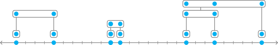
(a) Single-linkage clustering of full dataset

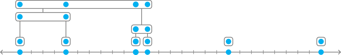
(b) Single-linkage clustering with one missing point

Figure 2: Figure 2(a) shows the single linkage clustering of $\mathcal{X}$, with three clusters $C_{1}$, $C_{2}$, and $C_{3}$ (left to right). In this example, $\zeta_{3,{\sf SL}}(\mathcal{X})=n$, as $d_{\sf mm}(C_{1}\cup C_{2};\mathcal{X})=6$ and $d_{\sf mm}(C_{3};\mathcal{X})=5$. There is a single point whose deletion dramatically changes the structure of the clustering in Figure 2(b).

In ${\sf SingleLinkage}$ (Algorithm 3), each $x\in\mathcal{X}$ is initially assigned its own cluster, as illustrated in Figure 2(a). At each iteration, the closest pairs of clusters are merged according to the inter-cluster distance $d(A,B)\stackrel{{\scriptstyle\textup{def}}}{{=}}\min_{x\in A,y\in B}d(x,y)$. ${\sf SingleLinkage}$ can be interpreted as a version of Kruskall’s algorithm for computing a minimum spanning tree: we may view $\mathcal{X}$ as a complete graph with the edge weight between $x,y\in\mathcal{X}$ equal to $d(x,y)$. In each iteration of the outer for loop, ${\sf SingleLinkage}$ increments a distance threshold $d_{i}$ and merges all points into a common cluster whenever there is a path between them with maximum edge weight at most $d_{i}$. The algorithm returns $k$ clusters corresponding to the $k$ connected components that Kruskall’s algorithm obtains. This perspective is formalized by the following notion of min-max distance and Lemma 4.2.

Definition 4.1.

The min-max distance between $x$ and $y$ is $d_{\sf mm}(x,y;\mathcal{X})=\min_{p}\max_{i}d(p_{i},p_{i+1})$, where the $\min$ is taken across all simple paths $p=(p_{1}=x,...,p_{t}=y)$ from $x$ to $y$ in the complete graph over $\mathcal{X}$. For $S\subset\mathcal{X}$, we also define $d_{\sf mm}(S;\mathcal{X})\stackrel{{\scriptstyle\textup{def}}}{{=}}\max_{x,y\in S}d_{\sf mm}(x,y;\mathcal{X})$.

Lemma 4.2.

Under ${\sf SingleLinkage}(\mathcal{X},k)$, $x,y\in\mathcal{X}$ are in the same cluster after the $\ell$-th round of the outer while loop if and only if $d_{\sf mm}(x,y;\mathcal{X})\leq d_{\ell}$.

Proof sketch.

We start with a graph of isolated nodes and add edges with weights equal to the minimum distances between nodes in differing components. Thus, two nodes will be connected after step $\ell$ if and only if there is a path between them with all edge weights at most $d_{\ell}$. ∎

Suppose we run ${\sf SingleLinkage}$ on a uniform random subsample $\mathcal{X}_{m}$ of $\mathcal{X}$ of size $m$. Lemma 4.2 shows that in ${\sf SingleLinkage}(\mathcal{X}_{m},k)$, clusters will be merged based on $d_{\sf mm}(x,y;\mathcal{X}_{m})$ (rather than $d_{\sf mm}(x,y;\mathcal{X})$). However, because subsampling $\mathcal{X}$ down to $\mathcal{X}_{m}$ can only decrease the number of paths and hence only increase the min-max distance between points, we have that $d_{\sf mm}(x,y;\mathcal{X}_{m})\geq d_{\sf mm}(x,y;\mathcal{X}).$ Consequently, if $d_{\sf mm}(x,y;\mathcal{X}_{m})$ is too much larger than $d_{\sf mm}(x,y;\mathcal{X})$ for certain pairs $x,y\in\mathcal{X},$ then the clustering outputted by ${\sf SingleLinkage}({\mathcal{X}_{m}},k)$ may be very different (and thus, have very different accuracy) from the clustering outputted by ${\sf SingleLinkage}(\mathcal{X},k).$ Meanwhile, if $d_{\sf mm}(x,y;\mathcal{X}_{m})$ appropriately approximates $d_{\sf mm}(x,y;\mathcal{X}),$ for most $x,y\in\mathcal{X}$, then we should expect ${\sf SingleLinkage}(\mathcal{X}_{m},k)$ and ${\sf SingleLinkage}(\mathcal{X},k)$ to return similar clustering.

Our main result in this section bounds the number of samples sufficient and necessary to ensure that ${\sf SingleLinkage}(\mathcal{X}_{m},k)$ and ${\sf SingleLinkage}(\mathcal{X},k)$ return similar clusterings. Our bound depends on a parameter $\zeta_{k,{\sf SL}}\in(0,n]$, defined as follows, with $\{C_{1},\dots,C_{k}\}={\sf SingleLinkage}(\mathcal{X},k)$:

$$\zeta_{k,{{\sf SL}}}(\mathcal{X})\stackrel{{\scriptstyle\textup{def}}}{{=}}n\left\lceil\frac{\min_{i,j\in[k]}d_{\sf mm}(C_{i}\cup C_{j};\mathcal{X})-\max_{t\in[k]}d_{\sf mm}(C_{t};\mathcal{X})}{\max_{t\in[k]}d_{\sf mm}(C_{t};\mathcal{X})}\right\rceil^{-1}.$$

To see why $\zeta_{k,{\sf SL}}\in(0,n]$ note that $C_{i},C_{j},C_{t}\in\mathcal{C}$ are clusters in the $k$-clustering of $\mathcal{X}$ while $C_{i}\cup C_{j}$ intersects two clusters ($C_{i}$ and $C_{j}$) contained in the $k$-clustering of $\mathcal{X}.$ So, Lemma 4.2 ensures that $\min_{i,j\in[k]}d_{\sf mm}(C_{i}\cup C_{j};\mathcal{X})-\max_{t\in[k]}d_{\sf mm}(C_{t};\mathcal{X})>0.$

We interpret $\zeta_{k,{{\sf SL}}}(\mathcal{X})$ as a natural measure of the stability of ${\sf SingleLinkage}$ on the dataset $\mathcal{X}$ with respect to random deletions. To understand why, suppose $\zeta_{k,{\sf SL}}(\mathcal{X})>\alpha\cdot n$ for some $\alpha\in(0,1]$. By rearranging the expression for $\zeta_{k,{\sf SL}}(\mathcal{X})$, we see that

$$\min_{i,j\in[k]}d_{\sf mm}(C_{i}\cup C_{j};\mathcal{X})>\frac{1}{\alpha}\cdot{\max_{t\in[k]}d_{\sf mm}(C_{t};\mathcal{X})}.$$

That is, the distance threshold required for merging $C_{i}\cup C_{j}$ into a single cluster is not too large relative to the distance threshold required to merge $C_{t}$ into a single cluster. This is illustrated in Figure 2(a) with $i=1$, $j=2$, and $t=3.$ When we subsample from $\mathcal{X}$ to build $\mathcal{X}_{m}$, there is some probability that we distort the min-max distance so that $d_{\sf mm}(C_{t};\mathcal{X}_{m})>d_{\sf mm}(C_{i}\cup C_{j};\mathcal{X}_{m}),$ causing ${\sf SingleLinkage}(\mathcal{X}_{m},k)$ to output a clustering that contains $C_{i}\cup C_{j}$ but does not contain $C_{t}$, as in Figure 2(b). If this occurs, we cannot expect size generalization to hold. Intuitively, when $\alpha$ is larger, the difference between $d_{\sf mm}(C_{t};\mathcal{X})$ and $d_{\sf mm}(C_{i}\cup C_{j};\mathcal{X}_{m})$ is smaller, and thus there is a higher probability $d_{\sf mm}(C_{t};\mathcal{X}_{m})>d_{\sf mm}(C_{i}\cup C_{j};\mathcal{X}_{m}).$ To control the probability of this bad event, we must take a larger value of $m$ in order to obtain size generalization with high probability.

We emphasize that $\zeta_{k,{\sf SL}}$ measures the stability of ${\sf SingleLinkage}$ on $\mathcal{X}$ with respect to point deletion, but it is fundamentally unrelated to the cost of ${\sf SingleLinkage}$ on $\mathcal{X}$ with respect to a ground truth (which is what we ultimately aim to approximate). Any assumption that $\zeta_{k,{\sf SL}}$ is small relative to $n$ does not constitute any assumptions that ${\sf SingleLinkage}$ achieves good accuracy on $\mathcal{X}$. Theorem 4.3 states our main result for size generalization of single linkage clustering.

Theorem 4.3.

Let $\mathcal{G}=\{G_{1},...,G_{k}\}$ be a ground-truth clustering of $\mathcal{X}$, $\mathcal{C}=\{C_{1},...,C_{k}\}={\sf SingleLinkage}(\mathcal{X},k)$, and $\mathcal{C}^{\prime}=\{C^{\prime}_{1},...,C^{\prime}_{k}\}={\sf SingleLinkage}(\mathcal{X}_{m},k)$. For

$$m={\tilde{O}\left(\left(\frac{k}{\epsilon^{2}}+\frac{n}{\min_{i\in[k]}\left\lvert C_{i}\right\rvert}+\zeta_{{k,{\sf SL}}}(\mathcal{X})\right)\log\frac{k}{\delta}\right)},$$

we have that $\operatorname*{\mathbb{P}}\left\{{\sf{cost}}_{\mathcal{G}}\left(\mathcal{C}^{\prime}\right)\approx_{\epsilon}{{\sf{cost}}_{\mathcal{G}}\left(\mathcal{C}\right)}\right\}\geq 1-\delta.$ Computing $\mathcal{C}^{\prime}$ requires $O(m^{2})$ calls to the distance oracle. Moreover, computing ${\sf{cost}}_{\mathcal{G}}\left(\mathcal{C}^{\prime}\right)$ requires only $m$ queries to the ground-truth oracle.

Proof sketch.

Let $H$ be the event that $\mathcal{C}^{\prime}$ is consistent with $\mathcal{C}$ on the subsample, i.e., there is a permutation $\sigma\in\Sigma_{k}$ such that for every $i\in[k]$, $C^{\prime}_{i}\subset C_{\sigma(i)}.$ If $H$ does not occur, we show $\exists S\subset\mathcal{X}_{m}$ such that $d_{\sf mm}(S;\mathcal{X}_{m})$ is significantly smaller than $d_{\sf mm}(S;\mathcal{X}).$ We lower bound the number of deletions required for this to occur and use this to lower the probability $H$ occurs. Conditioned on $H$, Hoeffding’s inequality implies a bound on the difference between ${\sf{cost}}_{\mathcal{G}}\left(\mathcal{C}^{\prime}\right)$ and ${{\sf{cost}}_{\mathcal{G}}\left(\mathcal{C}\right)}.$ ∎

When $\zeta_{k,{\sf SL}}(\mathcal{X})$ and $1/\left(\min_{i\in[k]}\left\lvert C_{i}\right\rvert\right)$ is small relative to $n$, Theorem 4.3 guarantees that a small subsample is sufficient to approximate the accuracy of single linkage clustering on the full dataset. We next provide lower bounds to illustrate a dependence on $\zeta_{k,{\sf SL}}(\mathcal{X})$ and $\min_{i\in[k]}\left\lvert C_{i}\right\rvert$ is necessary. In addition, we describe empirical studies of $\zeta_{k,{\sf SL}}$ on several natural data-generating distributions.

Dependence on cluster size $\min_{i\in[k]}\left\lvert C_{i}\right\rvert$.

Suppose our subsample entirely misses one of the clusters in $\mathcal{C}={\sf SingleLinkage}(\mathcal{X},k)$, (i.e., $\mathcal{X}_{m}\cap C_{i}=\emptyset$). Then ${\sf SingleLinkage}(\mathcal{X}_{m},k)$ will cluster $\mathcal{X}_{m}$ into $k$ clusters, while ${\sf SingleLinkage}(\mathcal{X},k)$ partitions $\mathcal{X}_{m}$ into at most $k-1$ clusters. Consequently, we can design ground truth on which clustering costs of $\mathcal{C}$ and $\mathcal{C}^{\prime}$ vary dramatically.

Lemma 4.4.

For any odd $n\geq 110$ and ${\gamma}>0$, there exists a $2$-clustering instance on $n$ nodes with a ground truth clustering $\mathcal{G}$ such that $\min_{i\in[k]}\left\lvert C_{i}\right\rvert=1$, $\zeta_{k,{\sf SL}}(\mathcal{X})\leq{\gamma}$ and with probability $.28$ for $m=n-1$, $\left\lvert{\sf{cost}}_{\mathcal{G}}\left({\sf SingleLinkage}(\mathcal{X}_{m},2)\right)-{\sf{cost}}_{\mathcal{G}}\left({\sf SingleLinkage}(\mathcal{X},2)\right)\right\rvert\geq 1/4.$

Dependence on $\zeta_{k,{\sf SL}}$.

The dependence on $\zeta_{k,{\sf SL}}(\mathcal{X})$ is also necessary and naturally captures the instability of ${\sf SingleLinkage}$ on a given dataset $\mathcal{X}$, as depicted in Figure 2. Lemma 4.5 formalizes a sense in which the dependence on the relative merge distance ratio $\zeta_{k,{\sf SL}}$ is unavoidable.

Lemma 4.5.

For any $n\geq 51$ with $n=1\textnormal{~{}mod~{}}3$, there exists a 2-clustering instance $\mathcal{X}$ on $n$ points such that $\zeta_{k,{\sf SL}}=n$; $\mathcal{C}={\sf SingleLinkage}(\mathcal{X},{2})$ satisfies $\min_{C\in\mathcal{C}}\left\lvert C\right\rvert\geq\frac{n}{6}$; and for $m=n-1$, with probability $.23$, $\left\lvert{\sf{cost}}_{\mathcal{G}}\left({\sf SingleLinkage}(\mathcal{X}_{m},{2})\right)-{\sf{cost}}_{\mathcal{G}}\left({\sf SingleLinkage}(\mathcal{X},{2})\right)\right\rvert\geq 1/12.$

Empirical study of $\zeta_{k,{\sf SL}}$.

We observe that for some natural distributions, such as when clusters are drawn from isotropic Gaussian mixture models, we can expect $\zeta_{k,{\sf SL}}$ to scale with the variance of the Gaussians. Intuitively, when the variance is smaller, the clusters will be more separated, so $\zeta_{k,{\sf SL}}$ will be smaller. We elaborate on these results in Appendix A.

5 Experiments

We present experiments on the following datasets.

MNIST:

The MNIST data generator from [10] generates instances consisting of handwritten digits. Ground truth classifications assign each image to the depicted digit.

Gaussian Mixtures (GM):

We generate from a 2-dimensional isotropic mixture model. With probability 1/2, points are sampled from the $\mathcal{N}((0,0)^{\top},.5\bm{I})$ or the $\mathcal{N}((1,1)^{\top},.5\bm{I})$ distribution. Ground truth classifications map points to the Gaussian from which they were generated.

Omniglot:

The Omniglot generator from [10] generates instances of handwritten characters from various languages. The ground truth maps characters to languages.

Noisy Circles (NC):

We use Pedregosa et al.’s [2011] noisy circles generator with noise level 0.05 and distance factor 0.2 to generate data consisting of concentric, noisy circles. Ground truth classifications map points to the circle to which they belong.

All instances contain $n$ points evenly split into $k=2$ clusters. For MNIST, GM, and NC, $n=200$. For Omniglot, $n=40$ (these instances are inherently smaller).

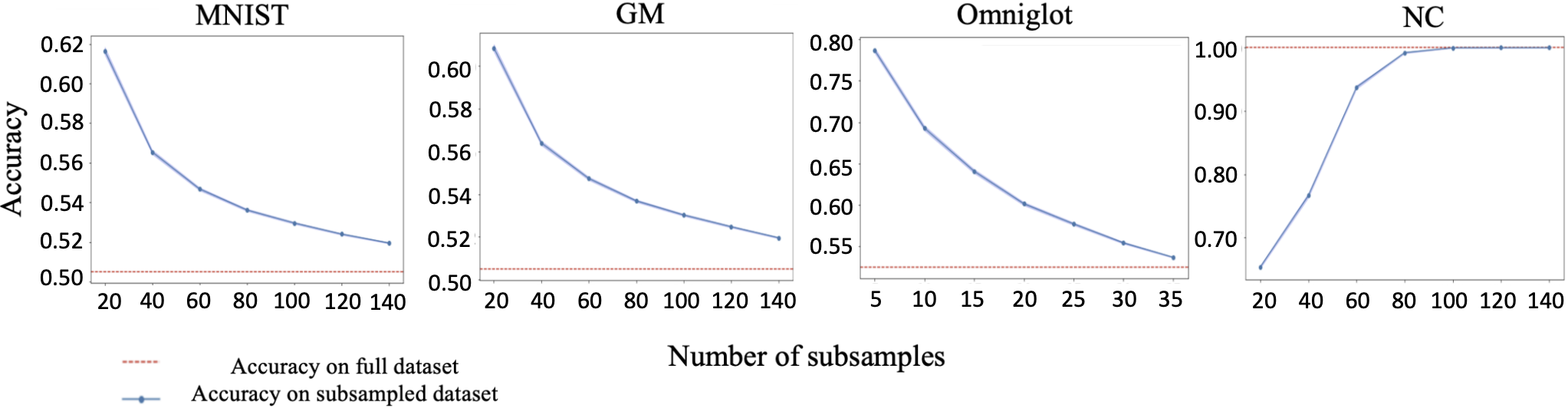
(a) Accuracy of subsampled SL and full-sample SL.

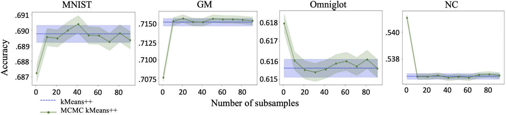
(b) Accuracy of MCMC-$k$-means++ approximation and $k$-means++ vs. $m$.

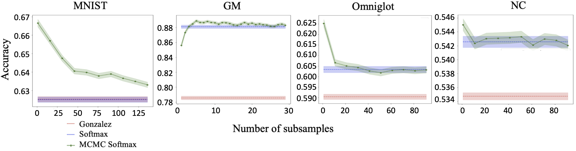
(c) Accuracy of MCMC-softmax approximation, softmax algorithm, and Gonzalez’s algorithm vs. $m$.

Figure 3: In Figures 3(a)-3(c), the proxy algorithms’ accuracies approach those of the original algorithms as the number of samples $m$ grows.

Figures 3(a)-3(c) compare the accuracy of the proxy algorithms from Sections 3 and 4 with the original algorithms run on the full dataset (averaged across $10^{4}$ repetitions), as a function of the number $m$ of randomly sampled clustering instances. The plots show 95% confidence intervals for the algorithms’ accuracies. The proxy algorithms’ accuracies approach those of the original algorithms as $m$ grows.

In Appendix B.2, we include additional plots pertaining to our empirical analysis of the softmax $k$-centers algorithm. Figure 8 compares the $k$-centers objective value of Gonzalez’s algorithm and our softmax $k$-centers algorithm (averaged over $10^{4}$ repetitions) as a function of $\beta$ for a randomly sampled instance. The objective value attained by softmax algorithm closely approximates or improves over Gonzalez’s algorithm even for small values of $\beta$. Figure 9 compares the $k$-centers objective value of Gonzalez’s algorithm softmax (averaged over $10^{5}$ repetitions) as a function of $n$ for fixed $\beta=1$ on randomly sampled GM, MNIST, and NC instances of $n$ points. Even with fixed $\beta$, the objective value of softmax closely tracks that of Gonzalez’s algorithm as $n$ increases.

6 Conclusion

To help narrow an important gap between theory and practice in the clustering literature, we introduce the notion of size generalization for estimating an algorithm’s accuracy. We prove size generalization guarantees for single linkage, $k$-means++, and a smooth variant of Gonzalez’s $k$-centers heuristic under natural assumptions on the clustering instances. An interesting question for future work is whether size generalization guarantees can be obtained for other clustering algorithms or combinatorial optimization problems (e.g., correlation clustering, max-cut, or max independent set.

Appendix A Key Challenges and Additional Related Work

In this section of the Appendix, we elaborate on our discussion from the introduction (Section 1). We first elaborate on additional related work in the context of our paper. Then, we provide figures illustrating the key challenges we mention in Section 1.

A.1 Additional related work

Algorithm selection.

Our work follows a line of research on algorithm selection. Practitioners typically utilize the following framework: (1) sample a training set of many problem instances from their application domain, (2) compute the performance of several candidate algorithms on each sampled instance, and (3) select the algorithm with the best average performance across the training set. This approach has led to breakthroughs in many fields, including SAT-solving [42], combinatorial auctions [33], and others [36, 21, 16]. On the theoretical side, [28] analyzed this framework from a PAC-learning perspective and applied it to several problems, including knapsack and max-independent-set. This PAC-learning framework has since been extended to other problems (for example, see [6] and the references therein). In this paper, we focus on step (2) of this framework in the context of clustering and study: when can we efficiently estimate the performance of a candidate clustering algorithm with respect to a ground truth?

Size generalization: gap between theory and practice.

There is a large body of research on using machine learning techniques such as graph neural networks and reinforcement learning for combinatorial optimization [e.g., 38, 26, 20, 30]. Typically, training the learning algorithm on small combinatorial problems is significantly more efficient than training on large problems. Many of these papers assume that the combinatorial instances are coming from a generating distribution [e.g., 38, 26, 20], such as a specific distribution over graphs. Others employ heuristics to shrink large instances [e.g., 30]. These approaches are not built on theoretical guarantees guaranteeing that an algorithm’s performance on the small instances is similar to its performance on the large instances. Our goal is to bridge this gap.

A.2 Illustrations of key challenges

Figure 4 provides an example of a dataset where the performance of $k$-means++ is extremely sensitive to the deletion or inclusion of a single point. This serves to illustrate that on worst-case datasets (e.g., with outliers or highly influential points) with worst-case ground truth clusterings, we cannot expect size generalization to hold.

Similarly, Figure 5 shows that on datasets without outliers, it may be possible to construct ground truth clusterings which are highly tailored to the performance of a particular clustering algorithm (such as Single Linkage) on the dataset. The figure shows that this type of adversarial ground truth clustering is a key challenge towards obtaining size generalization guarantees for clustering algorithms.

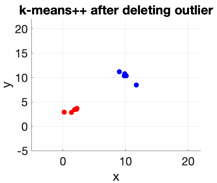
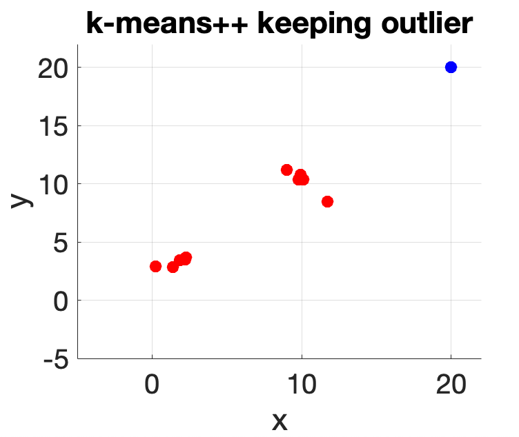
Figure 4: Sensitivity of $k$-means++ with respect to a single point. The example shows that the algorithm’s accuracy can be extremely sensitive to the presence or absence of a single point, in this case, the outlier at (20, 20). Depending on how the ground truth is defined, deleting the outlier can either boost or drop the accuracy by up to 50%.

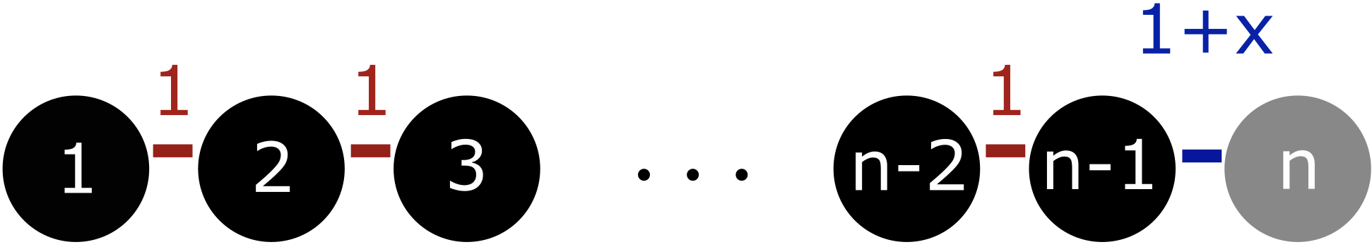
Figure 5: Example of a ground truth where size generalization by subsampling fails for single linkage. The shading indicates the ground truth. The first $n-1$ points are unit distance apart, while the last two points are $1+x>1$ distance apart. Single linkage has 0 cost on the full dataset. After randomly deleting a single point, the largest gap between consecutive points is equally likely to occur between any consecutive points. So, the expected cost on the subsample is $\geq\frac{1}{n}\sum_{i=2}^{n-1}\frac{(n-1-i)}{n}\overset{n\rightarrow\infty}{\rightarrow}1/2$.

Appendix B Additional Experimental Results

B.1 Empirical Results Supporting Section 4

We ran experiments to visualize $\zeta_{k,SL}(\mathcal{X})$ versus appropriate notions of noise in the dataset for two natural toy data generators. First, we considered isotropic Gaussian mixture models in $\mathbb{R}^{2}$ consisting fo two clusters centered at $(-2,-2)$ and $(2,2)$ respectively with variance $\sigma^{2}I$ (Figure 6.) Second, we considered 2-clustering instances drawn from scikitlearn’s noisy circles dataset with a distance factor of .5 and [34] with various noise levels (Figure 7.) In both cases $n=300$ points were drawn. Moreover, in both cases, we see that, as expected $\zeta_{k,{\sf SL}}$ grows with the noise in the datasets.

Figure 6: $\zeta_{k,{\sf SL}}$ vs $\sigma$ for isotropic Gaussian mixture model. The $y$-axis shows the average value of $\zeta_{k,{\sf SL}}(\mathcal{X})$ averaged over 30 draws of $\mathcal{X}$ for a given choice of $\sigma.$

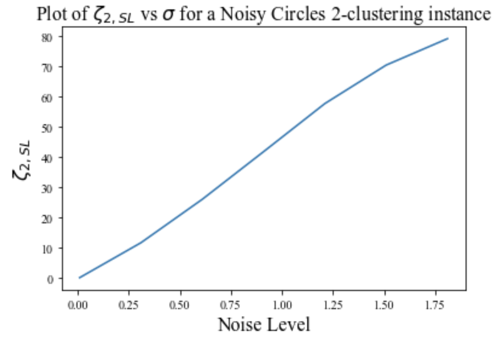
Figure 7: $\zeta_{k,{\sf SL}}$ vs $\sigma$ for noisy circle datasets. The $y$-axis shows the average value of $\zeta_{k,{\sf SL}}(\mathcal{X})$ averaged over 30 draws of $\mathcal{X}$ for a given choice of $\sigma.$

B.2 Empirical analysis of SoftmaxCenters

As discussed in Section 5, Figure 8 compares the $k$-centers objective value of Gonzalez’s algorithm and our softmax $k$-centers algorithm (averaged over $10^{4}$ repetitions) as a function of $\beta$ for a randomly sampled instance. The objective value attained by softmax algorithm closely approximates or improves over Gonzalez’s algorithm even for small values of $\beta$. Figure 9 compares the $k$-centers objective value of Gonzalez’s algorithm softmax (averaged over $10^{5}$ repetitions) as a function of $n$ for fixed $\beta=1$ on randomly sampled GM, MNIST, and NC instances of $n$ points. Even with fixed $\beta$, the objective value of softmax continues to closely track that of Gonzalez’s algorithm as $n$ increases.

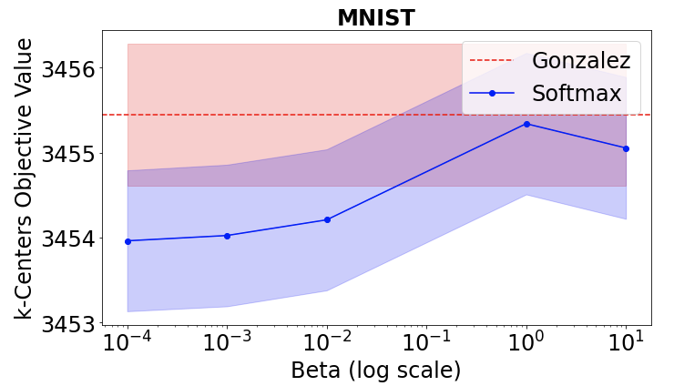
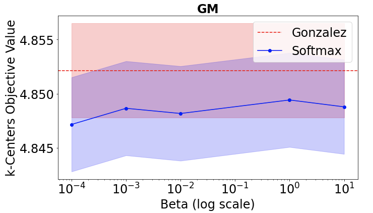
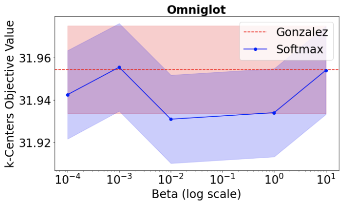
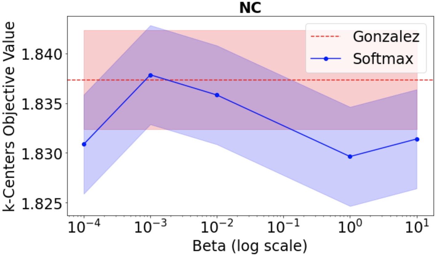
Figure 8: Objective value of softmax algorithm and of Gonzalez’s algorithm vs. $\beta$. The plot shows 95% confidence intervals for the algorithms’ $k$-centers objective values on randomly sampled instances. The softmax algorithm matches or improves over the objective value achieved by Gonzalez’s algorithm, even for small $\beta$.

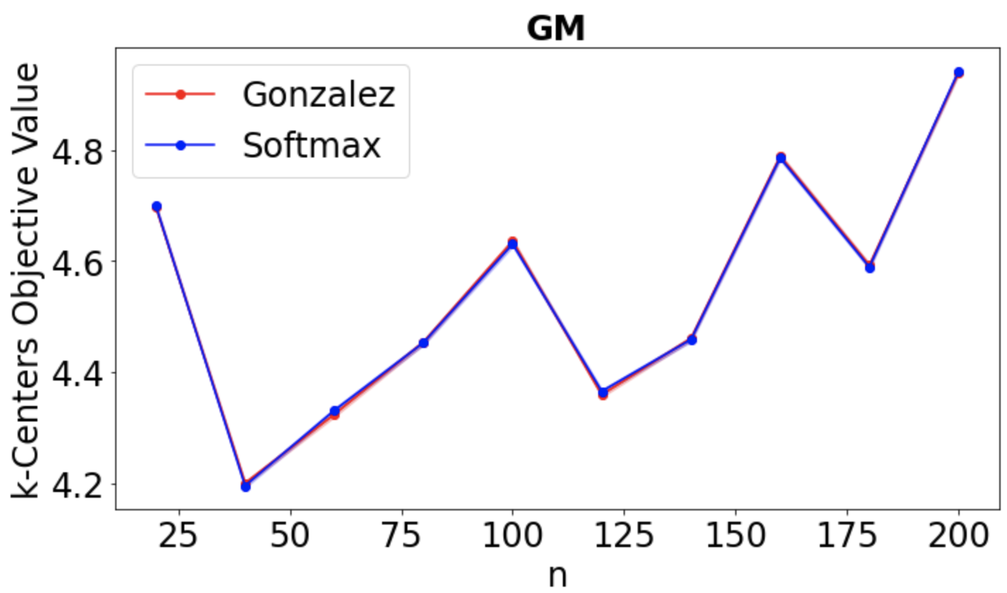
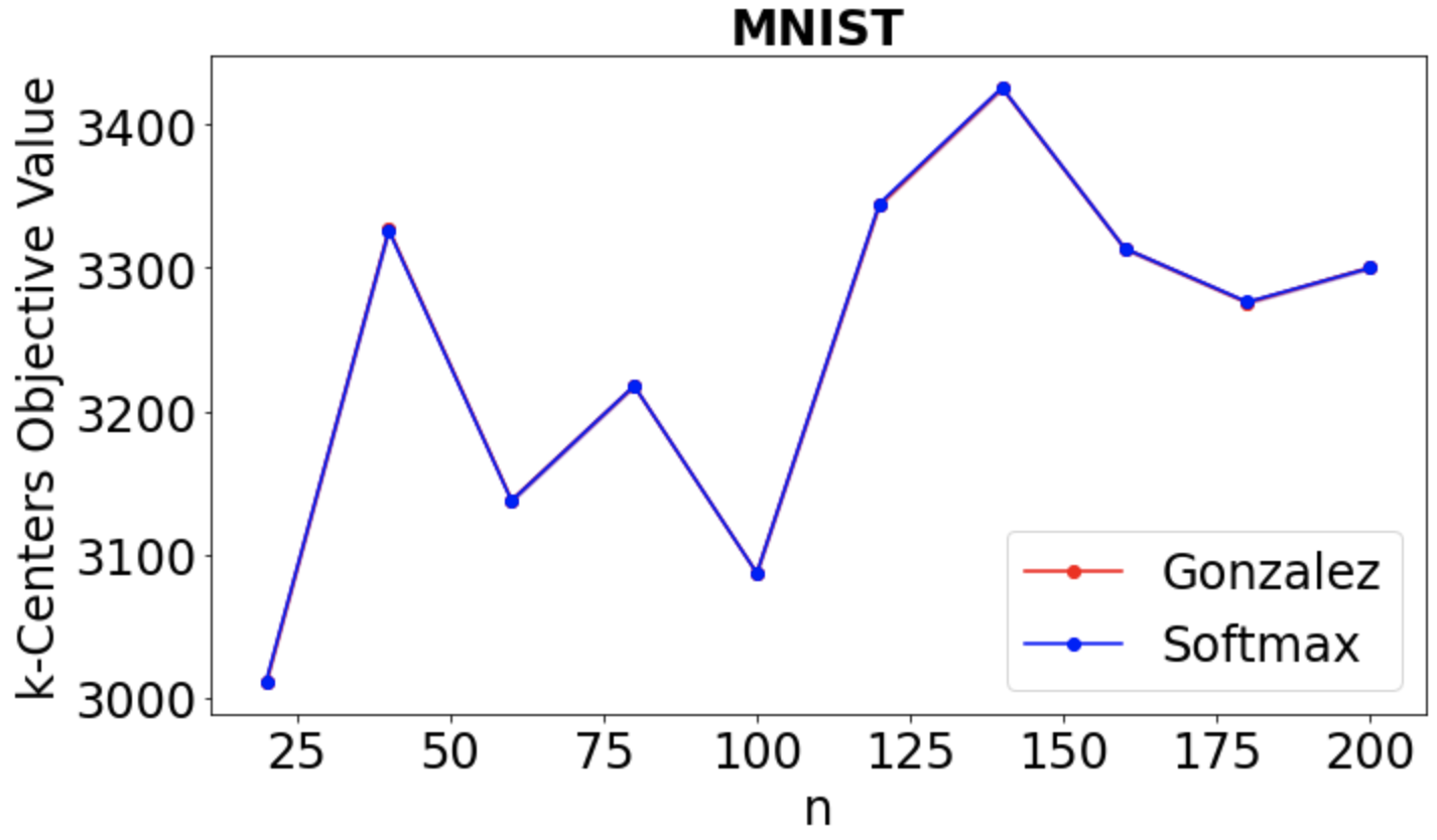
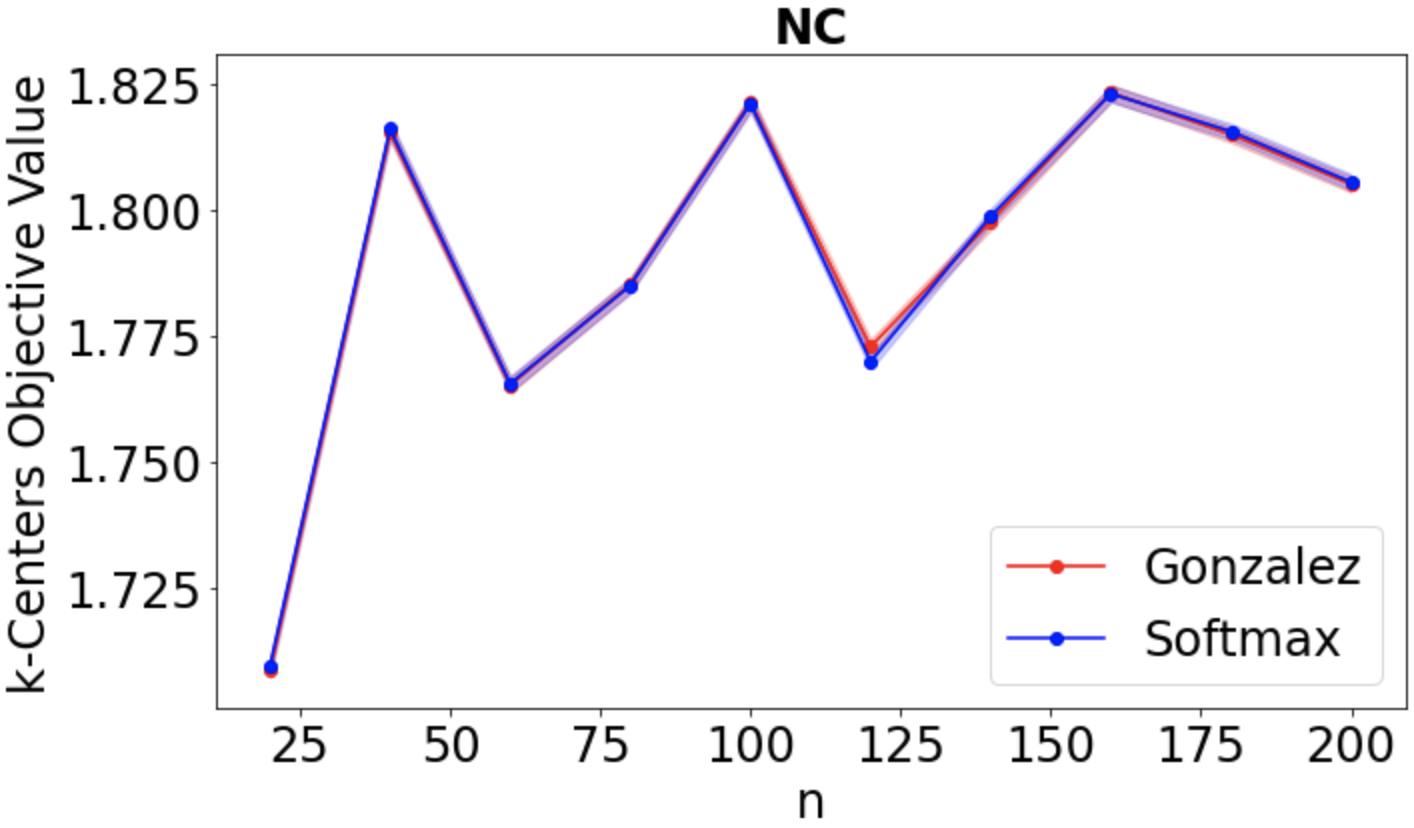
Figure 9: Objective of softmax algorithm and of Gonzalez’s algorithm vs. $n$ for $\beta=1$. The plot shows 95% confidence intervals for the algorithms’ $k$-centers objective values on randomly sampled instances of size $n$. The relative performance of softmax tracks the performance of Gonzalez’s algorithm extremely well as $n$ grows despite keeping the temperature $\beta$ fixed. (Omniglot was omitted in this figure because the instances are small.)

Appendix C Omitted Proofs

In Section C.1 we include proofs pertaining to our analysis of center-based clustering methods ($k$-means++ and $k$-centers.)

In Section C.2, we include omitted proofs pertaining to our analysis of single linkage clustering. In Section C.1 we include proofs pertaining to our analysis of center-based clustering methods ($k$-means++ and $k$-centers.)

C.1 Omitted Proofs from Section 3

In this section, we provide omitted proofs relating to our results on $k$-centers and $k$-means++ clustering. Throughout this section, we denote the total variation (TV) distance between two (discrete) distributions $p,q:\Omega\to[0,1]$ is $\left\lVert p-q\right\rVert_{TV}\stackrel{{\scriptstyle\textup{def}}}{{=}}\frac{1}{2}\sum_{\omega\in\Omega}\left\lvert p(\omega)-q(\omega)\right\rvert$. If $p(x,y)$ is the joint distribution of random variables $X$ and $Y$, $p_{X}(x)$ and $p_{Y}(y)$ denote the marginal distributions, and $p_{X|Y}(x|y)$ or $p_{Y|X}(y|x)$ denote the conditional distributions of $X|Y$ or $Y|X$, respectively.

Fact C.1.

Let $p,q$ be arbitrary, discrete joint distributions over random variables $X$ and $Y$ with conditionals and marginals denoted as follows: $p_{X,Y}(x,y)=p_{X}(x)\cdot p_{Y|X}(y|x)$ and $q_{X,Y}(x,y)=q_{X}(x)\cdot q_{Y|X}(y|x).$ If $\left\lVert p_{X}-q_{X}\right\rVert_{TV}\leq\epsilon_{1}$ and $\left\lVert p_{Y|X}-q_{Y|X}\right\rVert_{TV}\leq\epsilon_{2}$, then $\left\lVert p_{X,Y}-q_{X,Y}\right\rVert_{TV}\leq\epsilon_{1}+\epsilon_{2}$.

Proof.

For any $x,y$ we have

$$\left\lvert p_{X,Y}(x,y)-q_{X,Y}(x,y)\right\rvert =\left\lvert p_{X}(x)\cdot p_{Y|X}(y|x)-q_{X}(x)\cdot q_{Y|X}(y|x)\right\rvert$$

$$=\left\lvert p_{X}(x)\cdot p_{Y|X}(y|x)-(q_{X}(x)-p_{X}(x))\cdot q_{Y|X}(y|x)-p_{X}(x)\cdot q_{Y|X}(y|x)\right\rvert$$

$$=\left\lvert p_{X}(x)\cdot(p_{Y|X}(y|x)-q_{Y|X}(y|x))+q_{Y|X}(y|x)\cdot(q_{X}(x)-p_{X}(x))\right\rvert$$

$$\leq p_{X}(x)\cdot\left\lvert p_{Y|X}(y|x)-q_{Y|X}(y|x)\right\rvert+q_{Y|X}(y|x)\cdot\left\lvert q_{X}(x)-p_{X}(x)\right\rvert$$

Hence,

$$\left\lVert p_{X,Y}-q_{X,Y}\right\rVert_{TV} =\frac{1}{2}\sum_{x,y}\left\lvert p_{X,Y}(x,y)-q_{X,Y}(x,y)\right\rvert$$

$$\leq\sum_{x}p_{X}(x)\frac{1}{2}\sum_{y}\left\lvert p_{Y|X}(y|x)-q_{Y|X}(y|x)\right\rvert$$

$$+\frac{1}{2}\sum_{x}\left\lvert q_{X}(x)-p_{X}(x)\right\rvert\sum_{y}q_{Y|X}(y|x)$$

$$\leq\epsilon_{2}+\epsilon_{1}.$$

∎

See 3.1

Proof.

Let $p(C)$ be the probability of sampling a set of $k$ centers $C$ in ApxSeeding$(\mathcal{X},k,m,f)$ and $p^{\prime}(C)$ be the probability of sampling a set of $k$ centers $C$ in GeneralSeeding$(\mathcal{X},k,f)$. Likewise, let $p(c_{i}|C^{i-1})$ and $p^{\prime}(c_{i}|C^{i-1})$ be the probability of sampling $c_{i}$ as the $i$-th center given $C^{i-1}$ was selected up to the $(i-1)$-th step in ApxSeeding$(\mathcal{X},k,m,f)$ and ApxRandCenters$(\mathcal{X},k,f)$ respectively. We have that

$$p(C) =\frac{1}{n}\prod_{i=2}^{k}p(c_{i}|C^{i-1}),\text{ and }p^{\prime}(C)=\frac{1}{n}\prod_{i=2}^{k}p^{\prime}(c_{i}|C^{i-1}).$$

By Corollary 1 of [15], ApxSeeding (Algorithm 2) with $m=O({\zeta_{k,f}}(\mathcal{X})\log(k/\epsilon))$ is such that for all $C^{i-1}\subset\mathcal{X}$ with $\left\lvert C^{i-1}\right\rvert\leq k-1$,

$$\left\lVert p(\cdot|C^{i-1})-p^{\prime}(\cdot|C^{i-1})\right\rVert_{TV}\leq\frac{\epsilon}{k-1}.$$

By chaining Lemma C.1 over $i=2,...,k$, it follows that $\left\lVert p-p^{\prime}\right\rVert_{TV}\leq\epsilon$. Now, let $p(Z|c_{1})$ and $p^{\prime}(Z|c_{1})$ denote the probability of selecting centers $Z=\{z_{2},...,z_{k}\}$ in iterations $i=2,...,k$, conditioned on having selecting $c_{1}$ in the first iteration of Seeding and ApxSeeding respectively. Then,

$$p^{\prime}(Z|c_{1})-\left\lvert\left(p(Z|c_{1})-p^{\prime}(Z|c_{1})\right)\right\rvert\leq p(Z|c_{1})\leq p^{\prime}(Z|c_{1})+\left\lvert\left(p(Z|c_{1})-p^{\prime}(Z|c_{1})\right)\right\rvert.$$

Let $\mathcal{X}^{k-1}$ denote the set of all subsets of size $k-1$ in $\mathcal{X}$. Using the fact that the proportion of mislabeled points is always between 0 and 1, we then have that

$$\operatorname*{\mathbb{E}}\left[{\sf{cost}}_{G}\left(S\right)\right]=\sum_{c_{1}\in\mathcal{X}}\frac{1}{n}\sum_{Z\in\mathcal{X}^{k-1}}{\sf{cost}}_{G}\left(c_{1}\cup Z\right)p(Z|c_{1})$$

$$\leq\sum_{c_{1}\in\mathcal{X}}\frac{1}{n}\sum_{Z\in\mathcal{X}^{k-1}}{\sf{cost}}_{G}\left(c_{1}\cup Z\right)p^{\prime}(Z|c_{1})+\frac{1}{n}\sum_{c_{1}\in\mathcal{X}}\sum_{Z\in\mathcal{X}^{k-1}}{\sf{cost}}_{G}\left(c_{1}\cup Z\right)\left\lvert\left(p(Z|c_{1})-p^{\prime}(Z|c_{1})\right)\right\rvert$$

$$\leq\operatorname*{\mathbb{E}}\left[{\sf{cost}}_{G}\left(S^{\prime}\right)\right]+\frac{1}{n}\sum_{c_{1}\in\mathcal{X}}\sum_{Z\in\mathcal{X}^{k-1}}\left\lvert\left(p(Z|c_{1})-p^{\prime}(Z|c_{1})\right)\right\rvert\leq\operatorname*{\mathbb{E}}\left[{\sf{cost}}_{G}\left(S^{\prime}\right)\right]+\left\lVert p-p^{\prime}\right\rVert_{TV}$$

$$\leq\operatorname*{\mathbb{E}}\left[{\sf{cost}}_{G}\left(S^{\prime}\right)\right]+\epsilon.$$

By a symmetric argument, we obtain a lower bound

$$\operatorname*{\mathbb{E}}\left[{\sf{cost}}_{G}\left(S\right)\right]$$

$$=\sum_{c_{1}\in\mathcal{X}}\frac{1}{n}\sum_{Z\in\mathcal{X}^{k-1}}{\sf{cost}}_{G}\left(c_{1}\cup Z\right)p(Z|c_{1})$$

$$\geq\sum_{c_{1}\in\mathcal{X}}\frac{1}{n}\sum_{Z\in\mathcal{X}^{k-1}}{\sf{cost}}_{G}\left(c_{1}\cup Z\right)p^{\prime}(Z|c_{1})-\frac{1}{n}\sum_{c_{1}\in\mathcal{X}}\sum_{Z\in\mathcal{X}^{k-1}}{\sf{cost}}_{G}\left(c_{1}\cup Z\right)\left\lvert\left(p(Z|c_{1})-p^{\prime}(Z|c_{1})\right)\right\rvert$$

$$\geq\operatorname*{\mathbb{E}}\left[{\sf{cost}}_{G}\left(S^{\prime}\right)\right]-\frac{1}{n}\sum_{c_{1}\in\mathcal{X}}\sum_{Z\in\mathcal{X}^{k-1}}\left\lvert\left(p(Z|c_{1})-p^{\prime}(Z|c_{1})\right)\right\rvert\geq\operatorname*{\mathbb{E}}\left[{\sf{cost}}_{G}\left(S^{\prime}\right)\right]-\left\lVert p-p^{\prime}\right\rVert_{TV}$$

$$\geq\operatorname*{\mathbb{E}}\left[{\sf{cost}}_{G}\left(S^{\prime}\right)\right]-\epsilon.$$

Next, we can compute $\hat{c}_{\mathcal{G}}(S^{\prime})$ as follows. Let $\tau:\mathcal{X}\mapsto[k]$ be the mapping corresponding to the ground truth clustering (i.e., $\tau(x)=i$ if and only if $x\in G_{i}$.) Let $\mathcal{X}^{\prime}=\{x_{1},...,x_{\ell}\}$ be a fresh random sample of $\ell$ elements selected without replacement from $\mathcal{X}$, and let

$$\hat{c}_{\mathcal{G}}(S^{\prime})\stackrel{{\scriptstyle\textup{def}}}{{=}}\min_{\sigma\in\Sigma_{k}}\frac{1}{\ell}\sum_{x\in\mathcal{X}^{\prime}}\sum_{i\in[k]}\mathds{1}{\left\{x\in S^{\prime}_{\sigma(i)}\wedge x\notin G_{i}\right\}}.$$

Consider any $\sigma\in\Sigma_{k}$. Then,

$$\operatorname*{\mathbb{E}}\left[\frac{1}{\ell}\sum_{x\in\mathcal{X}^{\prime}}\sum_{i\in[k]}\mathds{1}{\left\{x\in S^{\prime}_{\sigma(i)}\wedge x\notin G_{i}\right\}}\right]=\frac{1}{n}\sum_{x\in\mathcal{X}}\sum_{i\in[k]}\mathds{1}{\left\{x\in S^{\prime}_{\sigma(i)}\wedge x\notin G_{i}\right\}}.$$

Hoeffding’s inequality guarantees that with probability ${\delta/k!}$,

$$\frac{1}{\ell}\sum_{x\in\mathcal{X}^{\prime}}\sum_{i\in[k]}\mathds{1}{\left\{x\in S^{\prime}_{\sigma(i)}\wedge x\notin G_{i}\right\}}\approx_{\epsilon}\frac{1}{n}\sum_{x\in\mathcal{X}}\sum_{i\in[k]}\mathds{1}{\left\{x\in S^{\prime}_{\sigma(i)}\wedge x\notin G_{i}\right\}}$$

for $l=O(k\epsilon^{-2}\log(k\delta^{-1}))$. The theorem follows by union bound over all $k!$ permutations $\sigma\in\Sigma_{k}$. ∎

See 3.2

Proof.

Let $S_{{\sf OPT}}=\{S_{1},...,S_{k}\}$ and $T=\{T_{1},...,T_{k}\}$. We use $S_{\sigma(i)}\in S$ to denote the partition such that $c_{i}\in S_{\sigma(i)}$ and $C^{(i-1)}\subset C$ to denote the centers chosen in the first $i-1$ iterations of SoftmaxCenters. We will show that for any $i\in\{2,...,k-1\}$, either $m_{i}\stackrel{{\scriptstyle\textup{def}}}{{=}}\max_{x\in\mathcal{X}}d(x;C^{(i-1)})\leq 4{\sf OPT}+\gamma$, or else with good probability, $c_{i}$ belongs to a different partition $S_{\sigma(i)}$ than any of $c_{1},...,c_{i-1}$ (i.e., $\sigma(i)\neq\sigma(j)$ for any $j<i$).

So, suppose $m_{i}>4{\sf OPT}+\gamma$, then let $B\stackrel{{\scriptstyle\textup{def}}}{{=}}\{x:x\in S_{\sigma(j)}\text{ for some }j<i\}$. We have

$$\operatorname*{\mathbb{P}}\left\{c_{i}\in B\right\}=\frac{\sum_{x\in B}\exp(\beta d(x;C^{(i-1)}))}{\sum_{x\in\mathcal{X}}\exp(\beta d(x;C^{(i-1)}))}.$$

For every $x\in S_{\sigma(j)}$, we know that $c_{j},s_{\sigma(j)}\in S_{\sigma(j)}$. By the triangle inequality, it follows that

$$d(x;C^{(i-1)})\leq d(x;c_{j})+d(c_{j},s_{\sigma(j)})\leq 2{\sf OPT}.$$

Consequently, using the fact that $g(z)=z/(z+c)$ is an increasing function of $z$ for $c>0$, we have

$$\operatorname*{\mathbb{P}}\left\{c_{i}\in B\right\}\leq\frac{|B|\exp(2\beta{\sf OPT})}{|B|\exp(2\beta{\sf OPT})+\sum_{x\in\mathcal{X}\setminus{B}}\exp(\beta d(x;C^{(i-1)}))}$$

Now, let $\ell\in[k]$ be the index of the optimal cluster in which $\exists y\in S_{\ell}$ with

$$d(y;C^{i})=m_{i}>4{\sf OPT}+\gamma.$$

Such an $\ell$ is guaranteed to exist, due to the assumption that $m_{i}>4{\sf OPT}+\gamma$. For $x\in S_{\ell}$ and $j<i$,

$$d(x;c_{j})+d(x,y) \geq d(y;c_{j})\geq 4{\sf OPT}+\gamma,$$

$$d(x,y) \leq 2{\sf OPT},$$

and hence $d(x;c_{j})\geq 2{\sf OPT}+\gamma$. So, it follows that

$$\operatorname*{\mathbb{P}}\left\{c_{i}\in B\right\} \leq\frac{|B|\exp(2\beta{\sf OPT})}{|B|\exp(2\beta{\sf OPT})+|S_{\ell}|\exp(\beta(2{\sf OPT}+\gamma))}=\frac{1}{1+\frac{|S_{\ell}|}{|B|}\exp(\beta(4{\sf OPT}+\gamma)-2{\sf OPT})}$$

$$\leq\frac{|B|}{|S_{\ell}|}\exp(-\beta\gamma)\leq k\mu_{u}/\mu_{l}\exp(-\beta\gamma)=\frac{\delta}{k}.$$

Now, by union bounding over $i=2,...,k$ we see that with probability at least $1-\delta$, either $m_{i}\leq 4{\sf OPT}+\gamma$ for some $i<[k]$; or, $\sigma(i)\neq\sigma(j)$ for any $j<i$.

In the former case, the approximation guarantee is satisfied. In the latter case, note that if every $c_{i}$ belongs to a distinct optimal cluster $S_{\sigma(i)}$, then every $x\in S_{\sigma(i)}$ for some $i\in[k]$. Consequently, by triangle inequality, we have that for any $x\in S_{\sigma(i)}$

$$d(x;C)\leq d(x;c_{i})\leq d(x,s_{\sigma(i)})+d(c_{i};s_{\sigma(j)})\leq 2{\sf OPT}<4{\sf OPT}+\gamma.$$

∎

See 3.4

Proof.

Consider $\mathcal{X}\subset[-R,R]$ such that $x_{1}=R$ and $x_{2},...,x_{n}=0$. By taking $Q=\{q_{1}=0,...,q_{k}=0\}$, we see that $\zeta_{k,{\sf SoftmaxCenters}}(\mathcal{X})\geq\frac{n\exp(\beta R)}{n-1+\exp(\beta R)}\geq\exp(\beta R)/2.$ ∎

C.2 Omitted Proofs from Section 4

In Section C.2.1, we present omitted proofs pertaining to size generalization of single linkage. In Section C.2.2, we present omitted proofs of our lower bounds.

C.2.1 Size generalization of single linkage clustering.

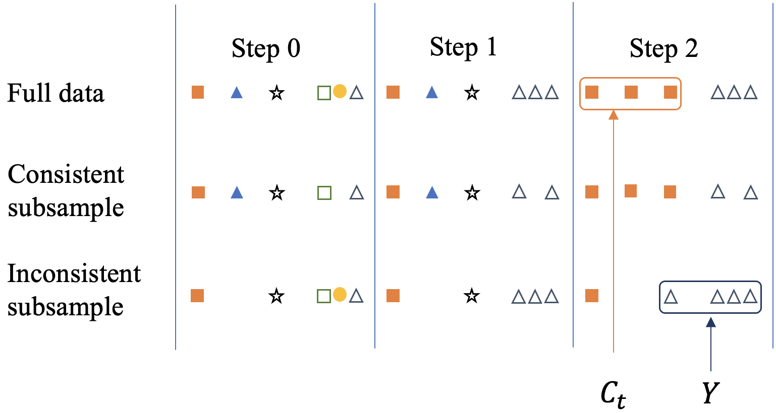
Figure 10: Examples of subsamples which induce a consistent and inconsistent clustering. The figure shows an example dataset $\mathcal{X}$ in one dimension along with the clustering $\mathcal{C}$ obtained by ${\sf SingleLinkage}(\mathcal{X},2)$ and ${\sf SingleLinkage}(\mathcal{X}_{m},2)$ on two different subsamples. Observe that second subsample produces an inconsistent clustering because the set $Y$ (1) has a nonempty intersection with both of the clusters from the full data and (2) gets merged into a single cluster at Step 4, before all points from $C_{t}$ have been merged together.

In this section, we provide omitted proofs relating to our results on single linkage clustering. We show that under natural assumptions on $\mathcal{X}$, running SingleLinkage on $\mathcal{X}$ yields similar accuracy as SingleLinkage on a uniform random subsample $\mathcal{X}_{m}$ of $\mathcal{X}$ of size $m$ (drawn with replacement) for $m$ sufficiently large.

We approach this analysis by showing that when $m$ is sufficiently large, the order in which clusters are merged in ${\sf SingleLinkage}(\mathcal{X},k)$ and ${\sf SingleLinkage}(\mathcal{X}_{m},k)$ is similar with high probability. Concretely, we show that for any subsets $S,T\subset\mathcal{X}_{m}$, the order in which $S$ and $T$ are merged is similar when we run ${\sf SingleLinkage}(\mathcal{X},k)$ and ${\sf SingleLinkage}(\mathcal{X}_{m},k)$. We use $d_{i}$ (respectively ${d_{m}}_{i}$) to denote the merge distance at iteration $i$ when running ${\sf SingleLinkage}(\mathcal{X},k)$ (respectively SingleLinkage $(\mathcal{X}_{m},k)$). Similarly, $\mathcal{C}^{i}$ (respectively $\mathcal{C}_{m}^{i}$) denotes the clustering at iteration $i$. We use $g_{m}(S)$ to denote the first iteration at which all points in $S$ are merged into a common cluster (we refer to this as the merge index of $S$). That is, $g_{m}:\mathcal{P}(\mathcal{X}_{m})\to[n-1]$ is a mapping such that for any $S\subset\mathcal{X}_{m}$, $g_{m}(S)=t$, where $t$ is the first iteration in ${\sf SingleLinkage}(\mathcal{X}_{m},k)$ such that $S\subset C$ for some $C\in{\mathcal{C}}^{t}_{m}$. Correspondingly, we use $d_{g(S)}$ and ${d_{m}}_{g_{m}(S)}$ denote the merge distance of $S\subset\mathcal{X}$ when running ${\sf SingleLinkage}$ on $\mathcal{X}$ and $\mathcal{X}_{m}$ respectively. Table 1 summarizes the notation used in our analysis.

Notation	Informal Description	Formal Definition
$g(S)$	The first iteration of the outer loop in ${\sf SingleLinkage}(\mathcal{X},k)$ at which all points in $S$ are merged into a single cluster.	For $S\subset\mathcal{X}$, $g(S)=\min\{\ell\in{\mathbb{Z}}_{\geq 0}:\exists C\subset\mathcal{C}^{\ell}\text{ such that }S\subset C\}$ when running ${\sf SingleLinkage}(\mathcal{X},k).$
$g_{m}(S)$	The first iteration of the outer loop in ${\sf SingleLinkage}(\mathcal{X}_{m},k)$ at which all points in $S$ are merged into a single cluster.	For $S\subset\mathcal{X}_{m}$, $g_{m}(S)=\min\{\ell\in{\mathbb{Z}}_{\geq 0}:\exists C\subset\mathcal{C}^{\ell}\text{ such that }S\subset C\}$ when running ${\sf SingleLinkage}(\mathcal{X}_{m},k).$
$d_{\ell}$	The merge distance at iteration $\ell$ of the outer loop in ${\sf SingleLinkage}(\mathcal{X},k)$	$\max_{i,j}\min_{x\in C_{i}^{(\ell-1)},y\in C_{j}^{(\ell-1)}}d(x,y).$ when running ${\sf SingleLinkage}(\mathcal{X},k).$
$d_{m_{\ell}}$	The merge distance at iteration $\ell$ of the outer loop in ${\sf SingleLinkage}(\mathcal{X}_{m},k)$	$\min_{i,j}\max_{x\in C_{i}^{(\ell-1)},y\in C_{j}^{(\ell-1)}}d(x,y).$ when running ${\sf SingleLinkage}(\mathcal{X}_{m},k).$

Table 1: Single linkage clustering analysis notation. The table summarizes key notation used in our analysis of single linkage clustering

We first prove Lemma 4.2, which characterizes when two points will be merged into a common cluster in single linkage clustering.

See 4.2

Proof.

For the forward direction, we will induct on the size of the cluster $C$. In the base case, if $\left\lvert C\right\rvert=2$, $C$ must be the result of merging some two clusters $A=\{x_{i}\},B=\{x_{j}\}$ such that $d(A,B)=d(x_{i},x_{j})\leq d_{t}\leq d_{\ell}$ at some iteration $t\leq\ell$. Therefore, $d_{\sf mm}(x_{i},x_{j};\mathcal{X})\leq d(x_{i},x_{j})\leq d_{\ell}$.

Now, assume that the statement holds whenever $\left\lvert C\right\rvert<m$. Then $\left\lvert C\right\rvert$ must be the result of merging some two clusters $A,B$ such that $\left\lvert A\right\rvert<m-1$, $\left\lvert B\right\rvert<m-1$, and $d(A,B)\leq d_{t}\leq d_{k}$ for some iteration $t\leq\ell$. Let $x_{i}\in A$ and $x_{j}\in B$ be two arbitrary points. Since $d(A,B)\leq d_{\ell}$, there exist $u\in A,v\in B$ such that $d(u,v)\leq d_{\ell}$. By inductive hypothesis, $d_{\sf mm}(x_{i},u;\mathcal{X})\leq d_{t}\leq d_{\ell}$ and $d_{\sf mm}(x_{j},v;\mathcal{X})\leq d_{t}\leq d_{\ell}$. Consequently, there exist paths $p_{1}\in\mathcal{P}_{x_{i},u},p_{2}\in\mathcal{P}_{x_{j},v}$ such that $p_{1}\cup(u,v)\cup p_{2}$ is a path between $x_{i}$ and $x_{j}$ with maximum distance between successive nodes at most $d_{\ell}$. Therefore, $d_{\sf mm}(x_{i},x_{j};\mathcal{X})\leq d_{\ell}$.

For the reverse direction, it is easy to see that after the merging step in iteration $k$, all nodes $u,v$ such that $d(u,v)\leq d_{k}$ must be in the same cluster. Consequently, if $d_{\sf mm}(x_{i},x_{j};\mathcal{X})\leq d_{k}$, there exists a path $p\in\mathcal{P}_{i,j}$ where $p=(v_{1}=x,v_{2},...,v_{k},v_{k+1}=x_{j})$ with $d({v_{i+1},v_{i}})\leq d_{k}$ for all $i\in[k]$. Consequently, all vertices on $p$ must be in the same cluster, and hence $x_{i},x_{j}\in C$ for some $C\in\mathcal{C}^{k}$. ∎

The analogous statement clearly holds for $\mathcal{X}_{m}$ as well, as formalized by the following corollary.

Corollary C.2.

Under ${\sf SingleLinkage}(\mathcal{X}_{m},k)$, $x,y\in\mathcal{X}_{m}$ are in the same cluster after the $\ell$-th round of the outer while loop if and only if $d_{\sf mm}(x,y;\mathcal{X}_{m})\leq d_{m_{\ell}}.$

Proof.

We repeat the identical argument used in Lemma 4.2 on $\mathcal{X}_{m}$. ∎

Lemma 4.2 and Corollary C.2 characterize the criteria under which points in $\mathcal{X}$ or $\mathcal{X}_{m}$ will be merged together in single linkage clustering. We can use these characterizations to obtain the following corollary, which relates $d_{g(S)}$ and $d_{m_{g}(S)}$ (see Table 1) to $d_{\sf mm}(S;\mathcal{X})$ and $d_{\sf mm}(S;\mathcal{X}_{m})$ respectively (recall Definition 4.1.)

Corollary C.3.

For any clustering instance $\mathcal{X}$ and set $S\subseteq\mathcal{X}$, $d_{g(S)}=\max_{x,y\in S}d_{\sf mm}(S;\mathcal{X}_{m})$. Likewise, for any $S\subseteq\mathcal{X}_{m}$, ${d_{m}}_{g_{m}(S)}=d_{\sf mm}(S;\mathcal{X}_{m})$.

Proof.

By definition, we know that on round $g(S)$, two sets $A$ and $B$ were merged where $S\subseteq A\cup B$ but $S\not\subseteq A$ and $S\not\subseteq B$. Moreover, $d_{g(S)}=\min_{x\in A,y\in B}d(x,y)$. We claim that for any $x\in S\cap A$ and $y\in S\cap B$, $d_{\sf mm}(x,y;\mathcal{X})\geq d_{g(S)}$. For a contradiction, suppose there exists $x\in S\cap A$ and $y\in S\cap B$ such that $d_{\sf mm}(x,y;\mathcal{X})<d_{g(S)}$. Then there exists a path $p$ between $x$ and $y$ such that for all elements $v_{i},v_{i+1}$ on that path, $d(v_{i},v_{i+1})<d_{g(S)}$. However, this path must include elements $v_{i},v_{i+1}$ such that $v_{i}\in A$ and $v_{i+1}\in B$, which contradicts the fact that $d_{g(S)}=\min_{x\in A,y\in B}d(x,y)$. Conversely, by Lemma 4.2, we know that for all $x,y\in S$, $d_{\sf mm}(x,y;\mathcal{X})\leq d_{g(S)}.$ Therefore, $d_{g(S)}=\max_{x,y\in S}d_{\sf mm}(x,y;\mathcal{X})$. The second statement follows by identical argument on $\mathcal{X}_{m}$. ∎

Our next step is to use Corollary C.3 to understand when the clustering $\mathcal{C}={\sf SingleLinkage}(\mathcal{X},k)$ and $\mathcal{C}^{\prime}={\sf SingleLinkage}(\mathcal{X}_{m},k)$ are “significantly” different. Concretely, our goal is to provide sufficient guarantees to ensure that $\mathcal{C}$ and $\mathcal{C}^{\prime}$ are consistent with each other on $\mathcal{X}_{m}$, i.e., that $\exists\sigma\in\Sigma_{k}$ such that for each cluster $C_{i}^{\prime}\in\mathcal{C}^{\prime}$, $C^{\prime}_{i}\subset C_{\sigma(i)}$. To aid in visualization, Figure 10 provides an example of a subsample $\mathcal{X}_{m}$ which induces a consistent clustering and an example of a subsample $\mathcal{X}_{m}$ which induces an inconsistent clustering.

Now, suppose, for example, that $\mathcal{C}^{\prime}$ is not consistent with $\mathcal{C}$ and let $C_{t}\in\mathcal{C}$ be the last cluster from $\mathcal{C}$ to be merged into a single cluster when running single linkage on the subsample $\mathcal{X}_{m}$. Since $\mathcal{C}^{\prime}$ and $\mathcal{C}$ are not consistent, there must be some cluster $Y\in\mathcal{C}^{\prime}$ which contains points from both of two other clusters. This means that when running ${\sf SingleLinkage}(\mathcal{X},k)$, $d_{g(Y)}>d_{g(C)}$ for all $C\in\mathcal{C}$. However, recall that since $Y\in\mathcal{C}^{\prime}$, when running ${\sf SingleLinkage}(\mathcal{X}_{m},k)$, there must exist some $C_{t}\in\mathcal{C}$ such that $d_{m_{g_{m}(Y)}}<d_{m_{g_{m}(C_{t})}}.$ Since $d_{g(Y)}>d_{g(C_{t})}$ but $d_{m_{g_{m}(Y)}}<d_{m_{g_{m}(C_{t})}}$, this means that when subsampling from $\mathcal{X}$ points, the subsample $\mathcal{X}_{m}$ must have distorted the min-max distances restricted to $C_{t}$ and $Y$. The following Lemma C.4 formalizes this observation.

Lemma C.4.

Suppose $T$ is merged into a single cluster under ${\sf SingleLinkage}(\mathcal{X}_{m},k)$ before $S$ is merged into a single cluster (i.e., $g_{m}(S)>g_{m}(T)$). Then there exists a pair of points $u,v\in S$ such that $d_{\sf mm}(u,v;\mathcal{X}_{m})-d_{\sf mm}(u,v;\mathcal{X})\geq d_{g(T)}-d_{g(S)}$.

Proof.

First, we argue that if $g(S)\geq g(T)$, then the statement is trivial. Indeed, if $g(S)\geq g(T)$, then for any $u,v\in\mathcal{X}$, $d_{\sf mm}(u,v;\mathcal{X}_{m})-d_{\sf mm}(u,v;\mathcal{X})\geq 0\geq d_{g(T)}-d_{g(S)}$. The first inequality is because any path in $\mathcal{X}_{m}$ clearly exists in $\mathcal{X}$, and the second inequality is because $d_{\ell}$ is non-decreasing in $\ell$.

On the other hand, if $g(S)<g(T)$, then Corollary C.3 indicates that

$$\max_{x,y\in S}d_{\sf mm}(x,y;\mathcal{X})=d_{g(S)}<d_{g(T)}=\max_{x,y\in T}d_{\sf mm}(x,y;\mathcal{X}).$$

Meanwhile, since $g_{m}(S)>g_{m}(T)$, there exists a pair of nodes $u,v\in S$ such that

$$d_{\sf mm}(u,v;\mathcal{X}_{m})=\max_{x,y\in S}d_{\sf mm}(x,y;\mathcal{X}_{m})>\max_{x,y\in T}d_{\sf mm}(x,y;\mathcal{X}_{m})\geq\max_{x,y\in T}d_{\sf mm}(x,y;\mathcal{X})=d_{g(T)}.$$

Finally, because $u,v\in S$, Corollary C.3 guarantees that $d_{\sf mm}(u,v;\mathcal{X})\leq d_{g(S)}$, we can conclude that $d_{\sf mm}(u,v;\mathcal{X}_{m})-d_{\sf mm}(u,v;\mathcal{X})>d_{g(T)}-d_{g(S)}.$ ∎

Lemma C.4 illustrates that the order in which sets in $\mathcal{X}_{m}$ are merged in ${\sf SingleLinkage}(\mathcal{X})$ and ${\sf SingleLinkage}(\mathcal{X}_{m})$ can differ only if some min-max distance is sufficiently distorted when points in $\mathcal{X}$ were deleted to construct $\mathcal{X}_{m}.$ In the remainder of the analysis, we essentially seek to show that large distortions in min-max distance are unlikely because they require deleting many consecutive points along a path. To this end, we first prove an auxiliary lemma, which bounds the probability of deleting $\ell$ points when drawing a uniform subsample of size $m$ with replacement from $n$ points.

Lemma C.5.

Let $S$ be a set of $n$ points and $S^{\prime}$ be a random subsample of $m$ points from $S$, drawn without replacement. Let $T=\{t_{1},...,t_{\ell}\}\subset S$. Then,

$$\exp\left(-\frac{m\ell}{(n-\ell)}\right)\leq\operatorname*{\mathbb{P}}\left\{T\cap S^{\prime}=\emptyset\right\}\leq\exp\left(-\frac{m\ell}{n}\right)\geq.2.$$

Proof.

Each sample, independently, does not contain $t_{i}$ for $i\in[\ell]$ with probability $1-\ell/n$. Thus,

$$\operatorname*{\mathbb{P}}\left\{T\cap S^{\prime}=\emptyset\right\} =\left(1-\frac{\ell}{n}\right)^{m}.$$

For the upper bound, we use the property that $(1-x/m)^{m}\leq\exp(-x)$:

$$\left(1-\frac{\ell}{n}\right)^{m}=\left(1-\frac{m\ell/n}{m}\right)^{m}\leq\exp\left(-\frac{m\ell}{n}\right).$$

Meanwhile, for the lower bound, we use the property that $\exp(-x/(1-x))\leq 1-x$ for $x\in[0,1]$:

$$\left(1-\frac{\ell}{n}\right)^{m}\geq\exp\left(-m\frac{\ell/n}{1-\ell/n}\right)=\exp\left(\frac{-m\ell}{n-\ell}\right).$$

∎

We can utilize the bound in Lemma C.5 to bound the probability of distorting the min-max distance between a pair of points by more than an additive factor $\eta$.

Lemma C.6.

For $\eta>0$ and $S\subset\mathcal{X}$,

$$\operatorname*{\mathbb{P}}\left\{\exists u,v\in\mathcal{X}_{m}\cap S:d_{\sf mm}(u,v;\mathcal{X}_{m})-d_{\sf mm}(u,v;\mathcal{X})>\eta\right\}\leq n^{3}\exp\left(-m\lceil\eta/d_{g(S)}\rceil/n\right).$$

Proof.

Suppose $\exists u,v\in\mathcal{X}_{m}\cap S$ such that $d_{\sf mm}(u,v;\mathcal{X}_{m})-d_{\sf mm}(u,v;\mathcal{X})>\eta$. Then, $\exists p=(u=p_{1},p_{2},...,p_{t}=v)\in\mathcal{P}_{u,v,\mathcal{X}}\setminus\mathcal{P}_{u,v,\mathcal{X}_{m}}$ with cost $\max_{i}d(p_{i},p_{i-1})=d_{\sf mm}(u,v;\mathcal{X})$. Since $t\leq n$ and $u,v\in S$, deleting any node $p_{i}\in p$ can increase the cost of this path by at most $d_{g(S)}$. Consequently, $\mathcal{X}_{m}$ must have deleted at least $s=\lceil{\eta}/{d_{g(S)}}\rceil$ consecutive points along $p$. There are at most $n$ distinct sets of $s$ consecutive points in $p$. Let $E_{i}$ be the event that $x_{1},...,x_{s}\notin\mathcal{X}_{m}$. Then, by Lemma C.5,

$$\operatorname*{\mathbb{P}}\left\{x_{1},...,x_{s}\notin\mathcal{X}_{m}\right\}\leq\exp\left(-\frac{ms}{n}\right).$$

The statement now follows by union bound over the $n$ distinct sets of $s$ consecutive points in $p$ and over the at most $n^{2}$ pairs of points $u,v\in S$. ∎

Finally, we can apply Lemma C.4 and Lemma C.6 to bound the probability that $\mathcal{C}^{\prime}$ and $\mathcal{C}$ are inconsistent.

Lemma C.7.

Let $\mathcal{C}=\{C_{1},...,C_{k}\}={\sf SingleLinkage}(\mathcal{X},k)$ and $\mathcal{C}^{\prime}=\{C^{\prime}_{1},...,C^{\prime}_{k}\}=$
${\sf SingleLinkage}(\mathcal{X}_{m},k)$. Let $\alpha_{ij}=d_{(g(C_{i}\cup C_{j}))}$ and $\alpha_{i}=d_{g(C_{i})}$. Let $E$ be the event that there exists a $C^{\prime}_{i}$ such that $C^{\prime}_{i}\not\subset C_{j}$ for all $j\in[k]$ (i.e., that $\mathcal{C}^{\prime}$ is inconsistent with $\mathcal{C}$; see Figure 10). Then,

$$\operatorname*{\mathbb{P}}\left\{E\right\}\leq(kn)^{3}\exp\left(-\frac{m}{n\zeta_{k,{\sf SL}}}\right)$$

Proof.

Let $S_{\ell}=C_{\ell}\cap\mathcal{X}_{m}$ for $\ell\in[k]$. Without loss of generality, we can assume that $i=1$. So, let $E_{a,b,j}$ be the event that $C_{1}^{\prime}\cap C_{a}\neq\emptyset\neq C_{1}^{\prime}\cap C_{b}$ and

$$g_{m}(C_{1}^{\prime})<g_{m}(S_{j}),\text{ and }g(S_{j})<g(C_{1}^{\prime}).$$

By Lemma C.4, this implies that there exists a $u,v\in S_{j}$ such that

$$d_{\sf mm}(u,v;\mathcal{X}_{m})-d_{\sf mm}(u,v;\mathcal{X})\geq d_{g(C_{1}^{\prime})}-d_{g(S_{j})}.$$

Since $C_{a},C_{b}\in\mathcal{C}$, we know that $g(C_{1}^{\prime})=g(C_{1}\cup C_{2})$. Meanwhile, $g(S_{j})=\alpha_{j}$, so we have

$$d_{\sf mm}(u,v;\mathcal{X}_{m})-d_{\sf mm}(u,v;\mathcal{X})\geq\alpha_{ab}-\alpha_{j}.$$

By Lemma C.6, it follows that

$$\operatorname*{\mathbb{P}}\left\{E_{a,b,j}\right\}\leq n^{3}\max_{a,b,j\in[k]}\exp\left(-\frac{m}{n}\left\lceil\frac{(\alpha_{ab}-\alpha_{j})}{\alpha_{j}}\right\rceil\right)=(kn)^{3}\exp\left(-\frac{m}{n\zeta_{k,{\sf SL}}}\right).$$

Now, $E=\bigvee_{a,b,j}E_{a,b,j}.$ By union bound over the at most $k^{3}$ configurations of $a,b,j$, the lemma follows. ∎

Finally, we can condition on the event that $\mathcal{C}$ and $\mathcal{C}^{\prime}$ are consistent to obtain our main result.

See 4.3

Proof.

Let $E$ be as defined in Lemma C.7 and let $F$ be the event that $\mathcal{X}\cap C_{i}=\emptyset$ for some $i\in\mathcal{X}$. Let $H=E\vee F$. $\operatorname*{\mathbb{P}}\left\{H\right\}\leq\operatorname*{\mathbb{P}}\left\{E\right\}+\operatorname*{\mathbb{P}}\left\{F\right\}$, where, by Lemma C.5,

$$\operatorname*{\mathbb{P}}\left\{F\right\}\leq k\max_{i}\operatorname*{\mathbb{P}}\left\{\mathcal{X}\cap C_{i}=\emptyset\right\}\leq k\exp\left(-\frac{m\cdot\min_{i\in[k]}\left\lvert C_{i}\right\rvert}{n}\right).$$

And by Lemma C.7, we have that

$$\operatorname*{\mathbb{P}}\left\{E\right\}\leq(nk)^{3}\exp\left(-\frac{m}{\zeta_{k,{\sf SL}}}\right).$$

We also have that

$$\operatorname*{\mathbb{P}}\left\{{\sf{cost}}_{\mathcal{G}}\left(\mathcal{C}^{\prime}\right)\approx_{\epsilon}{{\sf{cost}}_{\mathcal{G}}\left(\mathcal{C}\right)}\right\}\geq\operatorname*{\mathbb{P}}\left\{{\sf{cost}}_{\mathcal{G}}\left(\mathcal{C}^{\prime}\right)\approx_{\epsilon}{{\sf{cost}}_{\mathcal{G}}\left(\mathcal{C}\right)}|\bar{H}\right\}\operatorname*{\mathbb{P}}\left\{\bar{H}\right\}.$$

Now, let $\tau:\mathcal{X}\mapsto[k]$ be the mapping such that $\tau(x)=i$ if and only if $x\in G_{i}$. Consider any permutation $\sigma:[k]\to[k]$. If $\bar{H}$ occurs, then we know that every $C^{\prime}_{i}\subset C_{j_{i}}$ for some $j_{i}\in[k]$, and we know that each $C_{j}\cap\mathcal{X}_{m}\neq\emptyset$ for each $j\in[k]$. Consequently, there exists a permutation $\rho:[k]\mapsto[k]$ such that $C^{\prime}_{i}\subset C_{\rho(i)}$. Without loss of generality, we can assume that $\rho$ is the identity, i.e., that $x\in C_{i}\iff x\in C_{i}^{\prime}$ for any $x\in\mathcal{X}_{m}$ (or else reorder the sets in $\mathcal{C}$ such that this holds). So, conditioning on $\bar{H}$, we have

$$\frac{1}{m}\sum_{x\in\mathcal{X}_{m}}\sum_{i\in[k]}\mathds{1}{\left\{x\in C^{\prime}_{\sigma(i)}\wedge x\notin G_{i}\right\}} =\frac{1}{m}\sum_{x\in\mathcal{X}}\sum_{i\in[k]}\mathds{1}{\left\{x\in C^{\prime}_{\sigma(i)}\wedge x\notin G_{i}\wedge x\in\mathcal{X}_{m}\right\}}$$

$$=\frac{1}{m}\sum_{x\in\mathcal{X}}\sum_{i\in[k]}\mathds{1}{\left\{x\in C_{\sigma(i)}\wedge x\notin G_{i}\wedge x\in\mathcal{X}_{m}\right\}},$$

$$\operatorname*{\mathbb{E}}\left[\frac{1}{m}\sum_{x\in\mathcal{X}_{m}}\sum_{i\in[k]}\mathds{1}{\left\{x\in C^{\prime}_{\sigma(i)}\wedge x\notin G_{i}\right\}}\right] =\operatorname*{\mathbb{E}}\left[\frac{1}{m}\sum_{x\in\mathcal{X}}\sum_{i\in[k]}\mathds{1}{\left\{x\in C_{\sigma(i)}\wedge x\notin G_{i}\wedge x\in\mathcal{X}_{m}\right\}}\right]$$

$$=\frac{1}{m}\frac{m}{n}\cdot\operatorname*{\mathbb{E}}\left[\sum_{x\in\mathcal{X}}\sum_{i\in[k]}\mathds{1}{\left\{x\in C_{\sigma(i)}\wedge x\notin G_{i}\right\}}\right].$$

So, by Hoeffding’s inequality and union bound over the permutations $\tau$,

$$\operatorname*{\mathbb{P}}\left\{\left\lvert{\sf{cost}}_{\mathcal{G}}\left(\mathcal{C}^{\prime}\right)-{{\sf{cost}}_{\mathcal{G}}\left(\mathcal{C}\right)}\right\rvert\leq\epsilon|\bar{H}\right\}\geq 1-(k!)\exp\left(-2\epsilon^{2}m\right)\geq 1-k^{k}\exp\left(-2\epsilon^{2}m\right).$$

Consequently, by taking $m\geq O\left(k\epsilon^{-2}\log\left(k\delta^{-1}\right)\right)$, we can ensure that

$$\operatorname*{\mathbb{P}}\left\{{\sf{cost}}_{\mathcal{G}}\left(\mathcal{C}^{\prime}\right)\approx_{\epsilon}{{\sf{cost}}_{\mathcal{G}}\left(\mathcal{C}\right)}|\bar{H}\right\}\geq 1-\delta/2.$$

By taking $m\geq O\left(\max\left(\zeta_{k,{\sf SL}}(\mathcal{X})\log\left(nk\delta^{-1}\right),\frac{n}{\min_{i\in[k]}\left\lvert C_{i}\right\rvert^{2}}\log\left(\delta^{-1}\right)\right)\right)$ we can also ensure $\operatorname*{\mathbb{P}}\left\{\bar{H}\right\}\geq 1-\delta/2$. Hence, $\operatorname*{\mathbb{P}}\left\{{\sf{cost}}_{\mathcal{G}}\left(\mathcal{C}^{\prime}\right)\approx_{\epsilon}{{\sf{cost}}_{\mathcal{G}}\left(\mathcal{C}\right)}\right\}\geq 1-\delta.$ ∎

C.2.2 Lower bounds for size generalization of single linkage clustering

We now turn our attention to proving the lower bound results in Section 4. In the following, we use the notation $B_{\epsilon}(z)\stackrel{{\scriptstyle\textup{def}}}{{=}}\{z\in\mathbb{R}:\left\lVert x-z\right\rVert_{2}\leq\epsilon\}$ to denote an $\epsilon$-ball centered at $z$ and consider clustering with respect to the standard Euclidean metric $d(x,y)\stackrel{{\scriptstyle\textup{def}}}{{=}}\left\lVert x-y\right\rVert_{2}.$

See 4.4

Proof.

Consider $0<\alpha<1/2$ and the 2-clustering instance $\mathcal{X}=\{x_{1},...,x_{n-1},x_{n}\}\subset\mathbb{R}^{2}$ where $x_{1},...,x_{(n-1)/2}\in B_{\alpha}(0)$, $x_{(n-1)/2+1},...,x_{n-1}\in B_{\alpha}(3)$, and $x_{n}=6$. Suppose $\mathcal{G}=\{G_{1},G_{2}\}$ where $G_{1}=\{x_{1},...,x_{n-1}\}$ and $G_{2}=\{x_{n}\}$.

It is easy to see that ${\sf{cost}}_{\mathcal{G}}\left({\sf SingleLinkage}(\mathcal{X})\right)=0$, since $x_{n}$ is sufficiently far from $0$ and $3$ to ensure that $x_{n}$ will be the last point to be merged with any other point. Consider $m=n-1$. Now, whenever $x_{n}\notin\mathcal{X}_{m}$, and $\mathcal{X}_{m}\cap B_{\alpha}(0)\geq n/4$, and $\mathcal{X}_{m}\cap B_{\alpha}(3)\geq n/4$ we have that ${\sf{cost}}_{\mathcal{G}}\left({\sf SingleLinkage}(\mathcal{X}_{m})\right)\geq 1/4$, as the algorithm will separate the points in $B_{\alpha}(0)$ from those in $B_{\alpha}(3)$. We can lower bound the probability of this event as follows.

By Lemma C.5,

$$\operatorname*{\mathbb{P}}\left\{x_{n}\in\mathcal{X}_{m}\right\}\leq 1-\exp(-1)\leq 0.63.$$

By Chernoff bound,

$$\operatorname*{\mathbb{P}}\left\{B_{\alpha}(3)\cap\mathcal{X}_{m}\leq\frac{n}{4}\right\}=\operatorname*{\mathbb{P}}\left\{B_{\alpha}(0)\cap\mathcal{X}_{m}\leq\frac{n}{4}\right\} =\operatorname*{\mathbb{P}}\left\{B_{\alpha}(0)\cap\mathcal{X}_{m}\leq\frac{(n-1)^{2}}{2n}\cdot\frac{2n^{2}}{4(n-1)^{2}}\right\}$$

$$\leq\operatorname*{\mathbb{P}}\left\{B_{\alpha}(0)\cap\mathcal{X}_{m}\leq\frac{(n-1)^{2}}{2n}\cdot 2/3\right\}$$

$$\leq\exp\left(-\frac{(n-1)^{2}}{36n}\right)\leq.05.$$

Thus, $\operatorname*{\mathbb{P}}\left\{{\sf{cost}}_{\mathcal{G}}\left({\sf SingleLinkage}(\mathcal{X}_{m})\right)\geq 1/4\right\}\geq 1-0.73=.28.$ Moreover, note that because the failure probabilities analyzed above are independent of $\alpha$, we can ensure that $\zeta_{k,{\sf SL}}\leq\epsilon$ without affecting any of the failure probabilities, which are independent. ∎

See 4.5

Proof.

Take $\alpha>0$ and $2\alpha>\beta>\alpha$. Suppose $\mathcal{X}$ is composed of four sets $\mathcal{X}=L\cup\{b\}\cup M\cup R$, where the left points $x\in L$ satisfy $x=0$. The middle points $x\in M$ satisfy $x=2\alpha$, and the right points $x\in R$ satisfy $x=2{\cdot}\alpha+\beta$. $\left\lvert L\right\rvert=\left\lvert M\right\rvert=\left\lvert R\right\rvert=\frac{n-1}{3}$. The “bridge” point $b=\alpha$. Here,

$$\zeta_{k,{\sf SL}}(\mathcal{X})=n\lceil(\beta-\alpha)/\alpha\rceil^{-1}=n.$$

Suppose the ground truth clustering $\mathcal{G}$ is defined as $G_{1}=L\cup\{b\}\cup M$ and $G_{2}=R$. Since $\beta>\alpha$, single linkage achieves a cost of 0 on $\mathcal{X}$. Meanwhile, suppose that $b\notin\mathcal{X}_{m}$. Then, because the minmax distance between any point in $L$ and $M$ is now $2\alpha>\beta$, single linkage run on $\mathcal{X}_{m}$ will create one cluster for $L$ and one cluster for $M\cup R$. Provided that $\mathcal{X}_{m}$ contains at least $\frac{n-1}{6}$ points in $M$, this implies that single linkage will have a cost greater than or equal to $1/12$ on $\mathcal{X}_{m}$. It now remains to bound the probability of these simultaneous events. Let $E_{1}$ be the event that $b\notin\mathcal{X}_{m}$, and let $E_{2}$ be the event that $\left\lvert M\cap\mathcal{X}_{m}\right\rvert\geq\frac{n-1}{6}$. We have

$$\operatorname*{\mathbb{P}}\left\{E_{1}\wedge E_{2}\right\}=\operatorname*{\mathbb{P}}\left\{E_{1}\right\}\operatorname*{\mathbb{P}}\left\{E_{2}|E_{1}\right\}\geq\operatorname*{\mathbb{P}}\left\{E_{1}\right\}\operatorname*{\mathbb{P}}\left\{E_{2}\right\}.$$

This is because $E_{1}$ is the event of not including certain elements in $\mathcal{X}_{m}$ and $E_{2}$ is the probability of including certain elements in $\mathcal{X}_{m}$, so, $\operatorname*{\mathbb{P}}\left\{E_{2}|E_{1}\right\}\geq\operatorname*{\mathbb{P}}\left\{E_{2}\right\}$. Now, consider $m=n-1$. By Lemma C.5,

$$\operatorname*{\mathbb{P}}\left\{E_{1}\right\}\geq\exp\left(-m\frac{1}{(n-1)}\right)=\exp(-1)\geq.36.$$

Meanwhile, to analyze $\operatorname*{\mathbb{P}}\left\{E_{2}\right\}$ we can use a Chernoff bound to see that whenever $n>3$, we have $n>m>2/3n$, and consequently,

$$\operatorname*{\mathbb{P}}\left\{E_{2}\right\} =1-\operatorname*{\mathbb{P}}\left\{\left\lvert\mathcal{X}_{m}\cap M\right\rvert<\frac{n-1}{6}\right\}$$

$$=1-\operatorname*{\mathbb{P}}\left\{\left\lvert\mathcal{X}_{m}\cap M\right\rvert<\frac{n}{2m}\cdot\frac{m(n-1)}{3n}\right\}$$

$$=1-\operatorname*{\mathbb{P}}\left\{\left\lvert\mathcal{X}_{m}\cap M\right\rvert<\left(1-\frac{2m-n}{2m}\right)\cdot\frac{m(n-1)}{3n}\right\}$$

$$\geq 1-\exp\left(-\frac{(2m-n)^{2}}{2(2m)^{2}}\frac{m}{6}\right)$$

$$=1-\exp\left(-\frac{(n-2)^{2}}{8(n-1)^{2}}\frac{(n-1)}{6}\right)$$

$$=1-\exp\left(-\frac{(n-2)^{2}}{48(n-1)}\right).$$

where, in the fourth line, we substituted $\frac{m}{n}\cdot\frac{n-1}{3}\geq\frac{m}{n}\frac{n}{6}=\frac{m}{6}$. Then, whenever $n\geq 51$, we have that the argument in the exponential is at least 1. And hence,

$$\operatorname*{\mathbb{P}}\left\{E_{1}\wedge E_{2}\right\}\geq\exp(-1)\left(1-\exp(-1)\right)>.23.$$

So, the lemma follows by a union bound. ∎

References

- Arthur and Vassilvitskii [2007] David Arthur and Sergei Vassilvitskii. k-means++: the advantages of careful seeding. In Annual ACM-SIAM Symposium on Discrete Algorithms (SODA), 2007.