Estimation of Spectral Risk Measure for Left Truncated and Right Censored Data

Abstract

Left truncated and right censored data are encountered frequently in insurance loss data due to deductibles and policy limits. Risk estimation is an important task in insurance as it is a necessary step for determining premiums under various policy terms. Spectral risk measures are inherently coherent and have the benefit of connecting the risk measure to the user’s risk aversion. In this paper we study the estimation of spectral risk measure based on left truncated and right censored data. We propose a non parametric estimator of spectral risk measure using the product limit estimator and establish the asymptotic normality for our proposed estimator. We also develop an Edgeworth expansion of our proposed estimator. The bootstrap is employed to approximate the distribution of our proposed estimator and shown to be second order “accurate”. Monte Carlo studies are conducted to compare the proposed spectral risk measure estimator with the existing parametric and non parametric estimators for left truncated and right censored data. Based on our simulation study we estimate the exponential spectral risk measure for three data sets viz; Norwegian fire claims data set, Spain automobile insurance claims and French marine losses.

Key words: Spectral risk measure, Truncated and censored data, Nonparametric estimation, Asymptotic properties. JEL Code: C1, C130, C140, C150

1 Introduction

Insurance is a data-driven industry that focuses on detecting, quantifying, and protecting against extreme or unexpected events. It is common to encounter incomplete data in the form of truncation and censoring when dealing with insurance data. The most common are the left truncation and right censoring (see [Klugman et al.(2004)]). For example, ordinary insurance deductibles are a common example of left truncation. With typical insurance deductibles, policyholders are not compelled to notify the insurance company of losses that are less than the deductible sum. In this case, the insurer’s data is considered truncated because these losses would be covered by the policyholder and not reflected in the insurer’s data systems. Right censoring is a common occurrence when working with policy limits. When the actual damages exceed the policy limitations, the insurer’s reimbursement shall not exceed the policy limit, and the loss will be deemed right censored. Left truncated data also occurs in banking institutions where similar to insurance deductibles, operational losses below any threshold are not disclosed. The data truncation observed in operational risk was investigated by [Ergashev et al.(2016)]. The left truncation and right censoring can be defined as follows:

Left Truncation: When left truncation occurs, an observation that is less than or equal to $d$ is not recorded; however, if the observation is more than $d$, it is recorded at the observed value. Let, $X$ and $M$ be two random variables, where one represents the size of loss and the other represents the recorded value. Mathematically, it can be represented as:

$$M=\left\{\begin{array}[]{ll}\text{not\ recorded}&\quad X\leq d\\ X&\quad X>d.\end{array}\right.$$

Right Censoring: In case of right censoring $X$ is observed if it is less than $u$ and if $X$ is higher or equal to $u$ we observe $u$. Mathematically, it can be represented as:

$$M=\left\{\begin{array}[]{ll}X&\quad X\leq u\\ u&\quad X\geq u.\end{array}\right.$$

Measures of financial risk manifest themselves explicitly in many different types of insurance problems, including the setting of premiums and thresholds (e.g.,for deductibles and reinsurance cedance levels) (see [Dowd and Blake(2006)]). These measures are used to assess the riskiness of the probability distribution tail, which is an important task in insurance data analytics. The connection between actuarial and financial mathematics is striking here, as premium principles in an actuarial context correspond to risk measures in financial mathematics (see [Pichler(2015)]). A premium principle is a rule for assigning premiums to the insurance risks. There are various premium principles. For comprehensive discussion see [Pichler(2015)] and [Wang(1996)]). The net-premium principle is often regarded as the most authentic and equitable premium principle in actuarial practice ([Pichler(2015)]). An insurance firm using the net-premium concept will inevitably go bankrupt in the long term, even if it covers all its costs by collecting fees from clients. It is essential for the insurance sector to adhere to premium principles to ensure the company’s continued existence and ability to provide insurance coverage for clients’ future claims. Despite this interesting fact, the exact loss distribution is usually not known. Therefore, alternate premium principles have been created. Also the implementation of an appropriate premium principle or risk measure is a vital concern for the calculation of premium in the insurance industry.

A simple principle, ensuring risk-adjusted credibility premiums, is the distorted premium principle ([Wang(1996)]). This principle is advantageous for insurance firms because actuaries do not need to modify their tools to calculate premiums or reserves. Risk adjusted insurance prices by employing distorted probability measures have been discussed by [Wang and Young(1998)], [Heras et al.(2012)] and [Calderin-Ojeda et al.(2023)]. The distorted probability relates directly to a special class of risk measures, the spectral risk measures (SRMs) introduced in [Acerbi(2002)]. An important study of SRMs, although under the different name distortion functional, was provided in [Tsukahara(2009)]. The notions of premium principles through distorting probability measures, distortion functionals, and SRMs are fundamentally similar but differ only in sign conventions, leading to either a concave or convex representation (see [Gzyl and Mayoral(2008)]). The most important premium functional, is the conditional tail expectation (CTE) (in financial context alternative term is expected shortfall (ES)) (see [Heras et al.(2012)] and [Calderin-Ojeda et al.(2023)]).

Among the different types of risk measures, the coherent risk measures have been traditionally used in actuarial science (see [Calderin-Ojeda et al.(2023)]). [Artzner et al.(1999)] established the idea of coherent risk measure (see Appendix). The main characteristic that sets any coherent risk measure apart from other risk measure is subadditivity. We use the SRMs because they are coherent by nature and have the advantage of relating the risk measure to the user’s risk aversion (see [Acerbi(2002)]). [Acerbi(2002)] introduced the SRM, which is a weighted average of the quantiles of a loss distribution, the weights of which are determined by the user’s risk aversion. In addition to that, SRMs are comonotonic and law invariant (see [Gzyl and Mayoral(2008)]). Law invariance is crucial for applications since it is essential for a risk measure to be estimable from empirical data (see [Gzyl and Mayoral(2008)]).

Definition 1

Let, $\phi\in\mathcal{L}^{1}([0,1])$ be an admissible risk spectrum (see Appendix) and $X$ be a random loss variable. Then the SRM, according to [Gzyl and Mayoral(2008)], is defined by

$$M_{\phi}=\int_{0}^{1}\phi(u)F^{-1}_{X}(u)du,$$ (1)

where $\phi$ is called the Risk Aversion Function and $F^{-1}_{X}$ is the quantile function of $X$(see Appendix).

According to [Gzyl and Mayoral(2008)], any rational investor can use a new weight function profile $\phi$ to reflect their subjective risk aversion. It is apparent that if $\phi(u)=\frac{1}{1-p}1_{p\leq u\leq 1}$ then $M_{\phi}$ is the ES which is a SRM. However, value at risk (VaR) is not a SRM because it is not a coherent risk measure.

The estimation of SRMs is something that interests us. The estimating literature for distortion risk measures (DRMs) is more extensive than that for SRMs. This study focuses on SRM estimation when the data are left truncated and right censored (LTRC). The truncation and censoring reduces the sample size of the data and the actual sample size in unknown. Hence ignoring the truncation and censoring would result in inaccurate estimation of SRM which will affect in the assignment of premiums.

The first and most important task in tackling such problems is to find point estimates of SRMs and examine their variability. The simplest method we can use is the empirical non parametric technique. But this empirical approach is inefficient due to the scarcity of sample data in the tails (see [Brazauskas and Kleefeld(2016)]). [Kaiser and Brazauskas(2006)] discussed that parametric estimators, can considerably increase the efficiency of quantile based estimators. Various authors have studied the estimation methods of DRMs like VaR, ES, proportional hazards transform, Wang transform, and Gini shortfall for LTRC data using the parametric approach. [Upretee(2020)] discussed the empirical non parametric estimator and parametric estimators of various DRMs for LTRC data and concluded that parametric estimators are more efficient. Again it is well known that folded distributions are useful models in statistics. [Nadarajah and Bakar(2015)] introduced several new folded distributions and have discussed an application of the distributions to the left truncated Norwegian fire claims data set. In order to estimate the severity of Norwegian fire claims for the years $1981$ through $1992$, [Brazauskas and Kleefeld(2016)] used a number of parametric families.

But the most significant disadvantage of parametric estimators is that they are susceptible to initial modeling assumptions, resulting in model uncertainty. Therefore, we opt for the non parametric approach to estimate the SRM, as it is resistant to model risk. Based on the literature, it is evident that the product limit (PL) estimator ([Tsai et al.(1987)]) is a more suitable approach for handling LTRC data compared to the empirical distribution function. Various authors have studied the estimation of quantile-based risk measures using the PL estimator in the context of LTRC data. [Zhou et al.(2000)] investigated the estimation of a quantile function based on LTRC data by using the kernel smoothing method. [Liang et al.(2015)] studied the conditional quantile estimation based on LTRC data. The authors defined a generalized PL estimator to estimate the conditional quantile. [Shi et al.(2018)] proposed an improved PL estimator to estimate the quantile function for length biased and right censored data. Again from [Cheng et al.(2016)] we observe that the quantile regression model can also be applied to deal with the LTRC data. But we do not find any literature regarding the estimation of SRM using the PL estimator. When working with LTRC data, it is well understood that the PL quantile estimator is a natural estimator of quantile. Therefore, it is evident that the PL estimator is the most suitable method for estimating SRM in LTRC data (see [Tsukahara(2009)]).

This paper’s objective is to consider the PL estimator in the estimation of $M_{\phi}$ and establish the asymptotic normality of the estimator. Additionally, we approximate the distribution of our proposed estimator using the bootstrap method and derive the Edgeworth expansion. We showed that the bootstrap yields second-order accurate approximations (i.e., with error of size $o(n^{-1/2})$) to the distribution of our proposed estimator. Using Monte Carlo (MC) simulations, we compare the accuracy of our proposed estimators under certain conditions where sample size is $n$ and $k$ is the coefficient of absolute risk aversion. Our simulation study shows that, the proposed estimator outperforms other estimators mentioned in our study for small values of $n$ and $k$ when observations are i.i.d. If observations are dependent it outperforms for all $n$ and $k=5,\ 10$. When $n\geq 500$ our proposed estimator outperforms for all values of $k$, except for $k=100$. The paper is arranged as follows. In section 2 we propose the nonparametric estimator of $M_{\phi}$ using the PL estimator. In section 3 we establish the asymptotic normality and derive the Edgeworth expansion of the estimator. Also we investigate Efron’s bootstrap method ([Efron (1979)]) to approximate the distribution of the estimator and study its accuracy. In section 4 we compare the finite sample performance of our proposed estimator with various parametric and non parametric estimator available in the literature for LTRC data using MC simulations and report the findings. Repeated comparisons are made for various sample sizes, estimation methods and for two severity models and dependent case. We also conduct a simulation study, where we estimate the coverage probabilities of confidence intervals. Section 5 estimates the exponential SRM of three data sets based on our simulation study. Two left truncated data set viz: Norwegian Fire Claims, Spain Automobile Insurance Claims and one LTRC data set i.e. French Marine Losses. Finally, in section 6, we discuss the findings and give the concluding remarks.

2 Proposed estimator

In this section we briefly discuss the PL estimator under left truncation and right censoring and based on that we define our proposed estimator of SRM. Let, ($X,\ T,\ S$) be a random vector where $X$ be the variable of interest with cumulative distribution function (cdf) $F$; $T$ is a random left truncation with cdf $G$ and $S$ is a random right censoring with cdf $L$. We assume that $F$, $G$ and $L$ are continuous. $X$, $T$, $S$ are assumed to be mutually independent. Suppose, one can only observe the pair $Y=X\wedge S$ and $\delta=I(X\leq S)$. Under this restriction, the random variable $X$ is called right censored. Additionally, the triple ($Y,T,\delta$) is called an LTRC observation of $X$ if it is observed only when $Y\geq T$. Nothing is observed if $Y<T$. The conditional distribution

$$P[Y\leq y,T\leq t,\delta=q|T\leq Y],\text{for}\ y,\ t\in(-\infty,\infty),\ q=0\ \text{or}\ 1,$$

defines the LTRC model. Let, $\alpha=P(Y\geq T)>0$, and let $W$ denote the df of $Y$. If $X$ is independent of $S$ then $1-W=(1-F)(1-L)$.

Let, ($X_{i},\ T_{i},\ S_{i},\ \delta_{i}$), $1\leq i\leq N$ be a sequence of random vectors which are i.i.d. The size of the sample $n$ that was actually observed is random as a result of truncation, where $n\leq N$ and $N$ unknown. But we can regard the observed sample, ($X_{i},\ T_{i},\ S_{i},\ \delta_{i}$), $1\leq i\leq n$ as being generated by independent random variables $X_{i}$, $T_{i}$, $S_{i}$, $1\leq i\leq N$. From the SLLN, $\frac{n}{N}\rightarrow\alpha=P(Y\geq T)>0\ a.s.$

Now given the value of $n$, the data ($X_{i},T_{i},S_{i},\delta_{i}$) are still i.i.d. That is, ($Y_{i},T_{i},\delta_{i}$), $i=1,2,\cdots,n$ are i.i.d random samples of ($Y,T,\delta$) which is observed, but the joint distribution of $Y$ and $T$ becomes

$$H^{*}(y,t)=P(Y\leq y,T\leq t|T\leq Y).$$

[Woodroofe(1985)] pointed out that $F$ is identifiable only if certain requirements on the support of $F$ and $G$ are met. For any df $K$, let

$$a_{K}=\inf\{t:K(t)>0\}$$

and

$$b_{K}=\sup\{t:K(t)<1\}$$

denote the left- and right-endpoints of its support. For the LTRC data, $F$ is identifiable if $a_{G}\leq a_{W}$ and $b_{G}\leq b_{W}$.

Let,

$$C(z)=P(T\leq z\leq Y|T\leq Y)=\alpha^{-1}G(z)(1-W(z-))=\alpha^{-1}P(T\leq z\leq S)(1-F(z-)),$$ (2)

where $a_{W}\leq z<\infty$. $C$ can be estimated by its empirical estimator

$$C_{n}(z)=n^{-1}\sum_{i=1}^{n}I(T_{i}\leq z\leq Y_{i}).$$

Let, $b$ denote a constant less than $b_{W}$. From [Stute(1993)] we observe that though $C$ is strictly positive on $a_{G}<z<b_{W}$, $C_{n}$ may vanish for some $z\in(a_{G},\ b_{W})$. In particular, $C_{n}$ vanishes for all $z$ less than the smallest $T$ order statistics.

It is critical for LTRC data to be able to generate nonparametric estimates of various features of the df $F$. [Zhou et al.(2000)] defined the nonparametric maximum likelihood estimator of $F$, called the PL estimator, as

$$\widehat{F}(x)=\left\{\begin{array}[]{ll}1-\prod_{Y_{i}\leq x}\Big{[}\frac{nC_{n}(Y_{i})-1}{nC_{n}(Y_{i})}\Big{]}^{\delta_{i}}&\mathrm{for}\quad x<Y_{(n)}\\ 1&\mathrm{for}\quad x\geq Y_{(n)},\end{array}\right.$$ (3)

where $Y_{(n)}=\max(Y_{1},\ldots,Y_{n})$. The properties of $\widehat{F}$ have been studied by [Wang(1987)], [Lai and Ying(1991)], [Stute(1993)], [Zhou(1996)], and [Zhou and Yip(1999)]. Again, [Uzunoḡullari and Wang(1992)], [Gijbels and Wang’s(1993)], [Gu(1995)], [Sun(1997)], and [Sun and Zhou(1998)] investigated nonparametric estimates of $F$’s density and hazard rate. Based on equation (3) we propose the following estimator for $M_{\phi}$,

$$\widehat{M}_{Prod}=\int_{0}^{1}\phi(u)\widehat{F}^{-1}(u)du.$$ (4)

The asymptotic normality and the Edgeworth expansion of $\widehat{M}_{Prod}$ is established in the following section.

3 Distribution of the estimator

We prove the asymptotic normality and derive the Edgeworth expansion of $\widehat{M}_{Prod}$ in this section. Also, the bootstrap is employed to approximate the distribution of our proposed estimator $\widehat{M}_{Prod}$. In order to improve upon the normal approximation of a probability distribution, the Edgeworth expansion offers higher-order corrections. The method employed in our derivation of the desired Edgeworth expansion is first to approximate the $\widehat{M}_{Prod}$ by a $U$-statistic with some sufficiently small error term and then to apply the known results of the Edgeworth expansion for $U$-statistic ([Wang and Jing(2006)]) by checking the relevant conditions.

3.1 Asymptotic normality

In the current model, as discussed by [Zhou(1996)], let us consider the following assumptions:

Assumption 1: $a_{G}\leq a_{W}$, $b_{G}\leq b_{W}$.

Assumption 2: $\int_{a_{W}}^{\infty}\frac{dF(z)}{G^{2}(z)}<\infty$. Let,

$$W^{*}(y)=P(Y\leq y,\delta=1|T\leq Y),$$

and

$$W_{n}^{*}(y)=n^{-1}\sum_{i=1}^{n}I(Y_{i}\leq y,\delta_{i}=1).$$

Theorem 1

Let, assumptions 1, 2, and $a_{W}\leq F^{-1}(t)\leq b<b_{W}$ are satisfied. Then

$$\sqrt{n}(\widehat{M}_{Prod}-M_{\phi})\xrightarrow{\text{d}}N(0,\sigma^{2})$$

where

$$\sigma^{2}=\int_{0}^{1}\int_{0}^{1}\frac{(1-u)(1-v)}{f(F^{-1}(u))f(F^{-1}(v))}\Big{[}\int_{a_{W}}^{F^{-1}(u)}\frac{dW^{*}(y)}{C^{2}(y)}\int_{a_{W}}^{F^{-1}(v)}\frac{dW^{*}(y)}{C^{2}(y)}-uv\Big{]}\phi(u)\phi(v)dudv.$$ (5)

Proof: See Appendix.

Hence, from Theorem 1 we can say that our proposed estimator $\widehat{M}_{Prod}$ is asymptotically distributed with Gaussian behavior as the sample size goes up.

Remark 1

[Gijbels and Wang’s(1993)] density estimate can be used to replace the density $f$, and empirical estimates of all other unknown values can be used to replace their estimates to provide a consistent estimate of $\sigma^{2}$ (see [Zhou et al.(2000)]).

3.2 Edgeworth Expansion

For simplicity, we shall denote

$$V_{i}=\{Y_{i},\ T_{i},\ \delta_{i}\},\ i=1,\cdots,n.$$

For $i,\ j=1,\cdots,n$, let

$$\zeta(V_{i}\ ;\ x) = \frac{I[Y_{i}\leq x,\delta_{i}=1]}{C(Y_{i})}-\int_{a_{W}}^{x}\frac{I[T_{i}\leq y\leq Y_{i}]dW^{*}(y)}{C^{2}(y)}$$

$$\psi_{1}(V_{i},\ V_{j}\ ;\ x) = \frac{-I[Y_{i}\leq x]I[T_{j}\leq Y_{i}\leq Y_{j}]}{C^{2}(Y_{i})}$$

$$\psi_{2}(V_{i},\ V_{j}\ ;\ x) = \int_{a_{W}}^{x}\frac{I[T_{i}\leq y\leq Y_{i}]I[T_{j}\leq y\leq Y_{j}]dW^{*}(y)}{C^{3}(y)}$$

$$\psi(V_{i},\ V_{j}\ ;\ x) = \psi_{1}(V_{i},\ V_{j}\ ;\ x)\delta_{i}+\psi_{2}(V_{i},\ V_{j}\ ;\ x)-E[\psi_{1}(V_{i},\ V_{j}\ ;\ x)+\psi_{2}(V_{i},\ V_{j}\ ;\ x)|V_{i}]$$

$$h_{1}(V_{i},\ V_{j}\ ;\ x) = \zeta(V_{i}\ ;\ x)+\zeta(V_{j}\ ;\ x)-\zeta(V_{i}\ ;\ x)\zeta(V_{j}\ ;\ x)+\psi(V_{i},\ V_{j}\ ;\ x)+\psi(V_{j},\ V_{i}\ ;\ x)$$

$$\sigma_{0}^{2} = \int_{a_{W}}^{x}\frac{dW^{*}(y)}{C^{2}(y)}$$

$$\sigma_{1}^{2} = (1-x)^{2}\int_{a_{W}}^{F^{-1}(x)}\frac{dW^{*}(u)}{C^{2}(u)}$$

and

$$U^{(n)}=\frac{1}{n^{2}}\sum_{i<j}h_{1}(V_{i},\ V_{j}\ ;\ x).$$

It is easy to see that $U^{(n)}$ is a $U$-statistic with a symmetric kernel. Theorem 2 gives the $U$-statistic representation of our proposed estimator.

Theorem 2

Let, assumptions 1, 2, and $a_{W}\leq F^{-1}(t)\leq b<b_{W}$ are satisfied. Then

$$\widehat{M}_{Prod}-M_{\phi}=-\int_{0}^{1}\frac{1}{f(F^{-1}(u))}\Big{[}\frac{(1-u)}{n^{2}}\sum_{i<j}h_{1}(V_{i};\ V_{j};\ F^{-1}(u))-\frac{1-u}{2n}\int_{a_{W}}^{F^{-1}(u)}\frac{dW^{*}(x)}{C^{2}(x)}\Big{]}\phi(u)du+\alpha_{n}$$

with $P(\sqrt{n}|\alpha_{n}|>cn^{-1/2}\log{n}^{(-1)})=o(n^{-1/2})$.

Proof: See Appendix.

Now, similar to Lemma 2 in Appendix we obtain another lemma stated below.

Lemma 1

Under the conditions of Theorem 2, for any $a_{W}<F^{-1}(t)<b_{W}$, we have

$$\sup_{y}|P(\sqrt{n}\sigma_{01}^{-1}\frac{1}{n^{2}}\sum_{i<j}h_{1}(V_{i},V_{j};F^{-1}(x))\leq y)-E_{n1}(y)|=o(n^{-1/2}),$$

where

$$E_{n1}(y)=\Phi(y)-\frac{\kappa_{3}}{6}n^{-1/2}\phi_{1}(y)(y^{2}-1),\ \kappa_{3}=\frac{1}{\sigma_{01}^{3}}\Big{(}-\frac{15}{2}\sigma_{01}^{4}+\int_{a_{W}}^{F^{-1}(x)}\frac{dW^{*}(t)}{C^{3}(t)}\Big{)},$$

$$\sigma_{01}^{2}=\int_{a_{W}}^{F^{-1}(x)}\frac{dW^{*}(t)}{C^{2}(t)},$$

$\Phi$ is the standard normal distribution function, and $\phi_{1}$ is the standard normal density function.

Proof: The proof is exactly similar to that of Lemma 3 in [Chang (1991)] and hence omitted.

Theorem 3

Let, assumptions 1, 2, and $a_{W}\leq F^{-1}(t)\leq b<b_{W}$ are satisfied. Then

$$\sup_{y}|P(\sqrt{n}\sigma^{-1}(\widehat{M}_{Prod}-M_{\phi})\leq y)-E_{n2}(y)|=o(n^{-1/2}),$$

$$E_{n2}(y)=\Phi(y)-n^{-1/2}\phi(y)[\frac{\kappa_{3}}{6}(y^{2}-1)+\frac{1}{2}\sigma_{01}].$$

Proof: See Appendix.

Hence, Theorem 3 gives the Edgeworth expansion of our proposed estimator $\widehat{M}_{Prod}$.

3.3 Bootstrap Approximation

In this section we consider the Efron’s bootstrap ([Efron (1979)]) to obtain “good” approximations to the distribution of our proposed estimator $\widehat{M}_{Prod}$. To describe the bootstrap with LTRC, let ($Y_{i}^{*}$, $T_{i}^{*}$, $\delta_{i}^{*}$), $i=1,\cdots,n$, be a random sample obtained by drawing with replacement from the observations {$V_{i}$}, $i=1,\cdots,n$. Let, $P^{*}$ denote the bootstrap probability, given the sample {$V_{i}$}, $i=1,\cdots,n$. Let,

$$C_{n}^{*}=\frac{1}{n}\sum_{i=1}^{n}I[T_{i}^{*}\leq z\leq Y_{i}^{*}],$$

$$W_{n}^{*^{*}}(y)=\frac{1}{n}\sum_{i=1}^{n}I[Y_{i}^{*}\leq y,\delta_{i}^{*}=1].$$

Then, the bootstrap PL estimator $\widehat{F}^{*}(x)$ can be defined by

$$\widehat{F}^{*}(x)=\left\{\begin{array}[]{ll}1-\prod_{Y_{i}^{*}\leq x}\Big{[}\frac{nC_{n}^{*}(Y_{i}^{*})-1}{nC_{n}^{*}(Y_{i}^{*})}\Big{]}^{\delta_{i}^{*}}&\mathrm{for}\quad x<Y_{(n)}^{*}\\ 1&\mathrm{for}\quad x\geq Y_{(n)}^{*},\end{array}\right.$$

where $Y_{(n)}^{*}=\max(Y_{1}^{*},\ldots,Y_{n}^{*})$. The bootstrap version of our proposed estimator $\widehat{M}_{Prod}^{*}$ is given by

$$\widehat{M}_{Prod}^{*}=\int_{0}^{1}\phi(u)\widehat{F}^{*^{-1}}(u)du,$$

and $\sigma^{*^{2}}$ is the bootstrap variance. To investigate the performance of the bootstrap approximation, we shall first establish the Edgeworth expansion for the distribution of the bootstrap estimator $\widehat{M}_{Prod}^{*}$ in our next theorem.

Theorem 4

Under the assumption of Theorem (3), we have with probability 1 for any $a_{W}\leq F^{-1}(t)\leq b<b_{W}$

$$\sup_{y}|P^{*}(\sqrt{n}\sigma^{*^{-1}}(\widehat{M}_{Prod}^{*}-\widehat{M}_{Prod})\leq y)-P(\sqrt{n}\sigma^{-1}(\widehat{M}_{Prod}-M_{\phi})\leq y)|=o(n^{-1/2}).$$

Proof: See Appendix.

Remark 2

From Theorem (4), the distribution of the bootstrap $M_{Prod}$ estimator approximates its true distribution with an error term $o(n^{-1/2})$. By this result, the coverage error for the bootstrap confidence interval will be $o(n^{-1/2})$.

4 Simulations

In this section we study the impact of unreported events such as insurance deductibles and policy limits on the estimation of SRM. A Monte Carlo study is carried out to provide some small sample comparisons. We compare our proposed estimator $\widehat{M}_{Prod}$ with the non parametric and parametric estimators mentioned in [Upretee(2020)]. First we define the two severity distributions mentioned in [Upretee(2020)].

4.1 Independent case

Let, the random sample $X^{*}_{1},\cdots,X^{*}_{n}$ satisfy the following conditional event:

$$X^{*}_{i}\stackrel{{\scriptstyle\mathclap{\mbox{d}}}}{{=}}\{\min(X_{i},u)|X_{i}>d\},\ i=1,\cdots,n$$ (6)

where $d$ is the deductible and $u$ is the policy limit. The distribution function is given by

$$F_{*}(x)=\left\{\begin{array}[]{ll}0&\mathrm{for}\quad x\leq d\\ \frac{F(x)-F(d)}{1-F(d)}&\mathrm{for}\quad d<x<u\\ 1&\mathrm{for}\quad x\geq u.\end{array}\right.$$

Two severity distributions used in our simulation study are defined as follows:

1. Shifted Exponential Distribution: Let, the random variable $X$ follows a shifted exponential distribution with a location (shift) parameter $x_{0}>0$ and scale parameter $\theta>0$ and denote it as $X\sim\mathrm{Exp}(x_{0},\theta)$. The df is defined as

   $$F(x)=1-e^{-(x-x_{0})/\theta},\ x\geq x_{0}.$$

   For $X\sim\mathrm{Exp}(x_{0},\theta)$, we have $[F(x)-F(d)]/[1-F(d)]=1-e^{-(x-d)/\theta}$ for $d<x<u$ ($d>x_{0}$) and the quantile of $X^{*}$ is given by

   $$F^{-1}_{*}(p)=\left\{\begin{array}[]{ll}-\theta\mathrm{log}(1-p)+d&\mathrm{for}\quad 0\leq p<1-e^{-(u-d)/\theta},\\ u&\mathrm{for}\quad 1-e^{-(u-d)/\theta}\leq p\leq 1.\end{array}\right.$$

2. Pareto I Distribution: Let, the random variable $X$ follows a Pareto I distribution with a scale parameter $x_{0}>0$ and shape parameter $\alpha>0$ and denote it as $X\sim\mathrm{PaI}(x_{0},\alpha)$. The df is defined as

   $$F(x)=1-(x_{0}/x)^{\alpha},\ x\geq x_{0}.$$

   For $X\sim\mathrm{PaI}(x_{0},\alpha)$, we have $[F(x)-F(d)]/[1-F(d)]=1-(d/x)^{\alpha}$ for $d<x<u$ ($d>x_{0}$) and the quantile of $X^{*}$ is given by

   $$F^{-1}_{*}(x)=\left\{\begin{array}[]{ll}d(1-p)^{-1/\alpha}&\mathrm{for}\quad 0\leq p<1-(d/u)^{\alpha},\\ u&\mathrm{for}\quad 1-(d/u)^{\alpha}\leq p\leq 1.\end{array}\right.$$

We consider the truncation and censoring thresholds as mentioned in [Upretee(2020)]:

• $d=4.10^{3}$ (corresponds to the $95\%$ data truncation under $\mathrm{Exp}(x_{0}=10^{3},\theta=10^{3})$ and $93.8\%$ under $\mathrm{PaI}(x_{0}=10^{3},\alpha=2.0)$).

• $u=14.10^{3}$ (corresponds to the $0.0045\%$ data censoring under $F_{E}=\mathrm{Exp}(d=4.10^{3},\theta=10^{3})$ and $8.2\%$ under $F_{P}=\mathrm{PaI}(d=4.10^{3},\alpha=2.0)$).

Next, we define different non parametric and parametric estimators of SRM. We use the exponential risk aversion function defined by [Cotter and Dowd(2006)],

$$\phi(u)=\frac{ke^{-k(1-u)}}{1-e^{-k}}.$$ (7)

where $k\in(0,\infty)$ is the user’s coefficient of absolute risk aversion and hence we call it as exponential SRM. The absolute risk aversion coefficient $k$, like the confidence level in the VaR and ES, plays a significant part in SRMs. According to [Cotter and Dowd(2006)], the higher the value of $k$, the more we pay attention to higher losses in comparison to other losses.

1. Maximum Likelihood(ML) estimation([Upretee(2020)]) If $X\sim\mathrm{Exp}(x_{0},\theta)$ i.e. Shifted exponential distribution then the estimate of VaR is given by

   $$\mathrm{VaR}_{p,ML}=x_{0}-\hat{\theta}_{ML}\mathrm{log}(p),$$

   where

   $$\hat{\theta}_{ML}=\frac{\sum_{i=1}^{n}(x^{*}_{i}-d)1_{\{d<x^{*}_{i}<u\}}+(u-d)1_{\{x^{*}_{i}=u\}}}{\sum_{i=1}^{n}1_{\{d<x^{*}_{i}<u\}}}.$$

   If $X\sim\mathrm{PaI}(x_{0},\alpha)$ i.e. Pareto I distribution then the estimate of VaR is given by

   $$\mathrm{VaR}_{p,ML}=x_{0}p^{-1/\hat{\alpha}_{ML}},$$

   where

   $$\hat{\alpha}_{ML}=\frac{\sum_{i=1}^{n}1_{\{d<x^{*}_{i}<u\}}}{\sum_{i=1}^{n}\mathrm{log}(x^{*}_{i}/d)1_{\{d<x^{*}_{i}<u\}}+\mathrm{log}(u/d)\sum_{i=1}^{n}1_{\{x^{*}_{i}=u\}}}.$$

   Then the SRM estimator is given by

   $$\widehat{M}_{ML}=\int_{0}^{1}\phi(u)\mathrm{VaR}_{u,ML}du,$$ (8)

   where $\phi$ is given in (7).

2. Percentile Matching(PM) estimation([Upretee(2020)]) If $X\sim\mathrm{Exp}(x_{0},\theta)$ then the estimate of VaR is given by

   $$\mathrm{VaR}_{p,PM}=x_{0}-\hat{\theta}_{PM}\mathrm{log}(p),$$

   where

   $$\hat{\theta}_{PM}=\frac{\theta-x^{*}_{[np_{1}]}}{\mathrm{log}(1-p_{1})},\ for\ 0<p_{1}<1-e^{-(u-d)/\theta}.$$

   If $X\sim\mathrm{PaI}(x_{0},\alpha)$ then the estimate of VaR is given by

   $$\mathrm{VaR}_{p,PM}=x_{0}p^{-1/\hat{\alpha}_{PM}},$$

   where

   $$\hat{\alpha}_{PM}=\frac{\mathrm{log}(1-p_{1})}{\mathrm{log}(d/x^{*}_{[np_{1}]})},\ for\ 0<p_{1}<1-(d/u)^{\alpha}.$$

   Then the SRM estimator is given by

   $$\widehat{M}_{PM}=\int_{0}^{1}\phi(u)\mathrm{VaR}_{u,PM}du,$$ (9)

   where $\phi$ is given in (7).

3. Empirical(EMP)([Upretee(2020)]) For $0<p<\frac{F(x)-F(d)}{1-F(d)}\leq 1$, the empirical estimator of VaR is

   $$\mathrm{VaR}_{p,EMP}=x^{*}_{[np]}.$$

   Then the SRM estimator is given by

   $$\widehat{M}_{EMP}=\int_{0}^{1}\phi(u)\mathrm{VaR}_{u,EMP}du,$$ (10)

   where $\phi$ is given in (7).

4. Kernel estimator The kernel quantile estimator for LTRC data proposed by [Zhou et al.(2000)] is defined as follows

   $$\hat{Q}(t)=\frac{1}{h}\int_{0}^{1}\widehat{F}^{-1}K\left(\frac{x-t}{h}\right)dx,$$

   where $h$ is the bandwidth and $K$ is the kernel function. Then the kernel based estimator of SRM is defined as follows

   $$\widehat{M}_{\hat{Q}}=\int_{0}^{1}\phi(u)\hat{Q}(u)du,$$ (11)

   where $\phi$ is given in (7). The bandwidth $h=0.4$ is chosen based on the paper by [Liang et al.(2015)] and the kernel function is chosen as Epanechnikov kernel.

4.1.1 Simulation setting and results

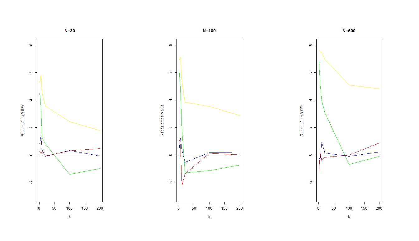
Figure 1: Logarithm of ratio of the MSEs for $F_{E}$ (black for $\widehat{M}_{Prod}$, blue for $\widehat{M}_{PM}$, red for $\widehat{M}_{ML}$, green for $\widehat{M}_{EMP}$, yellow for $\widehat{M}_{\hat{Q}}$).

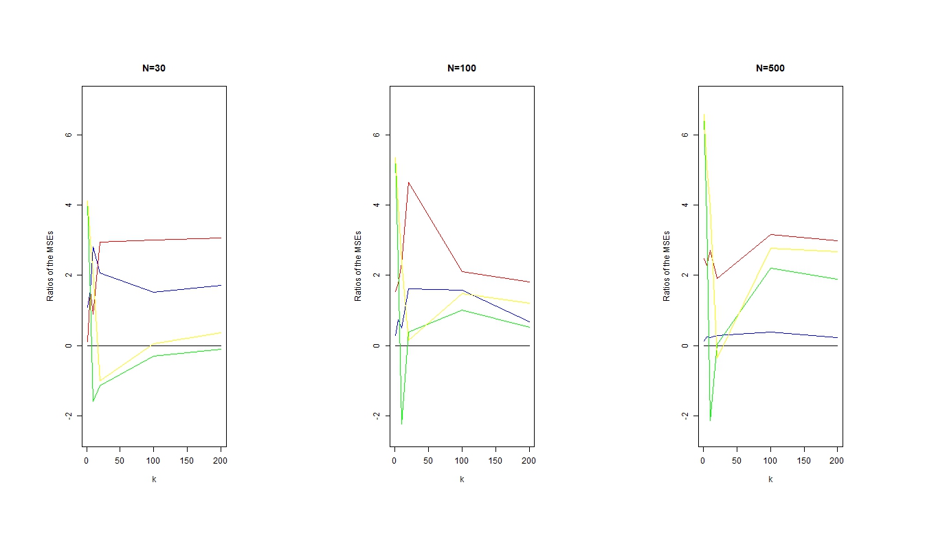
Figure 2: Logarithm of ratio of the MSEs for $F_{P}$ (black for $\widehat{M}_{Prod}$, blue for $\widehat{M}_{PM}$, red for $\widehat{M}_{ML}$, green for $\widehat{M}_{EMP}$, yellow for $\widehat{M}_{\hat{Q}}$).

From a specified LTRC severity distribution, we generate $10000$ samples of a specified length $n=30,\ 100,\ 500$ and for $k=1,\ 5,\ 10,\ 20,\ 100,\ 200$. For each sample, we estimate the SRM estimators defined in equation (4), (8), (9), (10) and (11). Then, based on those $10000$ SRM estimates, we compute their mean, standard deviation (SD) and mean squared error (MSE). In Table 1 and 2 we report the means, SDs and MSEs of the SRM estimates for the two distributions $F_{E}$ and $F_{P}$. All entries are measured in 1000’s. In Figure 1 and 2 we plot the logarithm of ratio of the MSEs (MSE of all the estimator is divided by the MSE of the $\widehat{M}_{Prod}$ estimator) of different SRM estimators for $F_{E}$ and $F_{P}$ distribution. From Table 1 and Figure 1 we observe that for $n=30$ and for all values of $k$ except for $k=20$ the $\widehat{M}_{Prod}$ estimator outperforms other estimators. For $n=100$ and for $k=1$ and $5$ the $\widehat{M}_{Prod}$ estimator outperforms all the estimators. When $n=500$ and $k=200$ the $\widehat{M}_{Prod}$ estimator outperform other estimators, but for other values of $k$ we see that $\widehat{M}_{ML}$ estimator outperform other estimators. Again, for $k=20$ and for all the sample sizes the $\widehat{M}_{ML}$ estimator also outperforms all the estimators. We also observe that when $k=100,\ 200$ and for all the sample sizes the $\widehat{M}_{EMP}$ estimator outperforms all the estimator. From Table 2 and Figure 2 we observe that for $n=30$ and $k=1,\ 5$ the $\widehat{M}_{Prod}$ estimator outperforms all the estimator in case of $F_{P}$ distribution. We even observe that for $n=100,\ 500$ and for all values of $k$ except for $k=10$, $\widehat{M}_{Prod}$ estimator outperforms all the estimator. We also observe that when $n=30$ and $k=10,\ 20,\ 100,\ 200$ the $\widehat{M}_{EMP}$ estimator outperforms other estimator. We observe that when $n=500$ the MSEs of $\widehat{M}_{Prod}$ and $\widehat{M}_{PM}$ estimator are very close to each other in case of $F_{P}$ distribution.

n	Estimation Methods	Estimated Values	$k=1$	$k=5$	$k=10$	$k=20$	$k=100$	$k=200$
	Theoretical Values		$2.260$	$3.203$	$3.878$	$4.572$	$6.182$	$6.876$
$30$	$\widehat{M}_{ML}$	Mean	$2.228$	$3.115$	$4.003$	$4.465$	$6.368$	$7.221$
		SD	$0.294$	$0.267$	$0.578$	$0.726$	$1.098$	$1.279$
		MSE	$87.460$	$79.033$	$349.709$	$538.525$	$1240.200$	$1754.866$
	$\widehat{M}_{PM}$	Mean	$2.177$	$3.253$	$3.539$	$4.199$	$6.217$	$6.653$
		SD	$0.374$	$0.524$	$0.519$	$0.630$	$1.115$	$0.986$
		MSE	$146.765$	$277.177$	$384.282$	$536.029$	$1244.450$	$1021.925$
	$\widehat{M}_{EMP}$	Mean	$4.716$	$4.720$	$4.811$	$5.713$	$6.012$	$6.562$
		SD	$0.188$	$0.179$	$0.182$	$0.183$	$0.436$	$0.603$
		MSE	$6067.280$	$2336.365$	$903.613$	$1335.370$	$218.996$	$413.338$
	$\widehat{M}_{Prod}$	Mean	$2.202$	$3.310$	$4.121$	$4.991$	$6.070$	$6.768$
		SD	$0.252$	$0.247$	$0.449$	$0.648$	$0.950$	$1.050$
		MSE	$66.868$	$72.458$	$260.650$	$595.465$	$915.044$	$1114.164$
	$\widehat{M}_{\hat{Q}}$	Mean	$5.899$	$7.966$	$8.707$	$9.110$	$9.396$	$9.430$
		SD	$0.145$	$0.078$	$0.075$	$0.099$	$0.111$	$0.122$
		MSE	$13263.346$	$22692.253$	$23320.037$	$20603.245$	$10342.117$	$6537.800$
$100$	$\widehat{M}_{ML}$	Mean	$2.237$	$3.177$	$3.861$	$4.701$	$6.190$	$6.779$
		SD	$0.201$	$0.187$	$0.108$	$0.299$	$0.558$	$0.572$
		MSE	$40.930$	$35.645$	$11.953$	$106.042$	$311.428$	$336.143$
	$\widehat{M}_{PM}$	Mean	$2.228$	$3.148$	$3.828$	$4.508$	$6.053$	$6.729$
		SD	$0.135$	$0.235$	$0.396$	$0.492$	$0.553$	$0.627$
		MSE	$19.249$	$58.250$	$159.316$	$246.160$	$322.450$	$412.234$
	$\widehat{M}_{EMP}$	Mean	$4.698$	$4.699$	$4.700$	$4.896$	$6.047$	$6.726$
		SD	$0.095$	$0.099$	$0.105$	$0.095$	$0.263$	$0.372$
		MSE	$5952.869$	$2247.817$	$686.709$	$114.001$	$87.394$	$160.884$
	$\widehat{M}_{Prod}$	Mean	$2.312$	$3.220$	$4.019$	$4.020$	$6.020$	$6.919$
		SD	$0.101$	$0.130$	$0.304$	$0.346$	$0.499$	$0.580$
		MSE	$12.905$	$17.189$	$112.297$	$424.420$	$275.245$	$338.249$
	$\widehat{M}_{\hat{Q}}$	Mean	$5.789$	$7.824$	$8.638$	$8.992$	$9.246$	$9.299$
		SD	$0.015$	$0.016$	$0.033$	$0.017$	$0.028$	$0.018$
		MSE	$12454.066$	$21353.897$	$22658.689$	$19536.689$	$9388.880$	$5871.253$
$500$	$\widehat{M}_{ML}$	Mean	$2.276$	$3.154$	$3.882$	$4.563$	$6.316$	$6.765$
		SD	$0.042$	$0.105$	$0.093$	$0.124$	$0.176$	$0.315$
		MSE	$1.780$	$13.426$	$8.665$	$15.457$	$48.941$	$111.546$
	$\widehat{M}_{PM}$	Mean	$2.273$	$3.212$	$3.827$	$4.588$	$6.204$	$6.901$
		SD	$0.068$	$0.089$	$0.175$	$0.145$	$0.210$	$0.238$
		MSE	$4.793$	$8.002$	$33.226$	$21.281$	$44.584$	$57.269$
	$\widehat{M}_{EMP}$	Mean	$4.596$	$4.609$	$4.695$	$5.201$	$6.078$	$6.766$
		SD	$0.044$	$0.044$	$0.048$	$0.043$	$0.119$	$0.172$
		MSE	$5458.832$	$1978.772$	$669.793$	$397.490$	$24.977$	$41.684$
	$\widehat{M}_{Prod}$	Mean	$2.308$	$3.284$	$3.909$	$4.612$	$6.283$	$6.819$
		SD	$0.060$	$0.071$	$0.110$	$0.130$	$0.200$	$0.209$
		MSE	$5.904$	$11.602$	$13.061$	$18.5$	$50.201$	$46.930$
	$\widehat{M}_{\hat{Q}}$	Mean	$5.758$	$7.803$	$8.593$	$8.964$	$9.214$	$9.260$
		SD	$0.002$	$0.009$	$0.005$	$0.009$	$0.005$	$0.003$
		MSE	$12236.008$	$21160.081$	$22231.250$	$19289.745$	$8099.741$	$5683.465$

• Notes: Estimates are measured in 1000’s.

Table 1: Mean, SD & MSE of SRM estimators for $F_{E}=Exp(x_{0}=10^{3},\theta=10^{3})$ distribution.

n	Estimation Methods	Estimated Values	$k=1$	$k=5$	$k=10$	$k=20$	$k=100$	$k=200$
	Theoretical Values		$2.363$	$3.984$	$5.605$	$7.927$	$17.725$	$24.066$
$30$	$\widehat{M}_{ML}$	Mean	$2.469$	$4.610$	$6.501$	$12.653$	$34.498$	$53.617$
		SD	$0.470$	$1.902$	$1.638$	$8.869$	$32.004$	$54.988$
		MSE	$232.136$	$4009.480$	$3485.860$	$100994.237$	$1326077.145$	$3111006.304$
	$\widehat{M}_{PM}$	Mean	$2.280$	$3.330$	$5.343$	$7.561$	$17.134$	$24.493$
		SD	$0.471$	$0.949$	$1.986$	$3.289$	$9.984$	$15.827$
		MSE	$228.730$	$1328.317$	$4012.840$	$10951.477$	$100029.537$	$250676.258$
	$\widehat{M}_{EMP}$	Mean	$5.719$	$5.729$	$5.746$	$6.719$	$11.037$	$12.701$
		SD	$0.540$	$0.526$	$0.520$	$0.492$	$1.961$	$1.584$
		MSE	$11554.336$	$3321.701$	$290.281$	$1708.585$	$48574.865$	$131672.281$
	$\widehat{M}_{Prod}$	Mean	$2.539$	$4.009$	$5.140$	$8.002$	$17.643$	$24.139$
		SD	$0.422$	$0.918$	$1.102$	$2.305$	$8.104$	$12.100$
		MSE	$209.060$	$843.349$	$1430.629$	$5318.650$	$65681.540$	$146415.329$
	$\widehat{M}_{\hat{Q}}$	Mean	$5.954$	$8.005$	$8.978$	$9.284$	$9.447$	$9.615$
		SD	$0.120$	$0.188$	$0.221$	$0.311$	$0.135$	$0.196$
		MSE	$12909.681$	$16203.785$	$11425.970$	$1938.170$	$68543.509$	$208869.817$
$100$	$\widehat{M}_{ML}$	Mean	$2.671$	$4.951$	$7.982$	$10.993$	$25.073$	$35.235$
		SD	$0.410$	$0.838$	$1.856$	$2.835$	$8.823$	$16.445$
		MSE	$262.964$	$1637.333$	$9094.865$	$112097.626$	$131838.433$	$395184.586$
	$\widehat{M}_{PM}$	Mean	$2.364$	$3.578$	$5.542$	$7.767$	$18.523$	$24.865$
		SD	$0.275$	$0.648$	$1.202$	$2.317$	$8.852$	$11.251$
		MSE	$75.626$	$584.740$	$1448.773$	$5394.089$	$78994.708$	$127223.402$
	$\widehat{M}_{EMP}$	Mean	$5.680$	$5.690$	$5.699$	$6.701$	$11.207$	$13.642$
		SD	$0.288$	$0.288$	$0.293$	$0.285$	$1.317$	$0.702$
		MSE	$11085.433$	$2993.380$	$94.685$	$1584.301$	$44218.813$	$109152.580$
	$\widehat{M}_{Prod}$	Mean	$2.431$	$3.941$	$5.739$	$7.810$	$17.739$	$24.041$
		SD	$0.229$	$0.528$	$0.927$	$1.029$	$4.028$	$8.030$
		MSE	$57.065$	$280.633$	$877.285$	$1072.530$	$16224.980$	$64481.525$
	$\widehat{M}_{\hat{Q}}$	Mean	$5.822$	$7.863$	$8.714$	$9.044$	$9.288$	$9.352$
		SD	$0.035$	$0.038$	$0.050$	$0.043$	$0.044$	$0.086$
		MSE	$11965.906$	$15048.085$	$9668.381$	$1249.538$	$71184.905$	$216509.192$
$500$	$\widehat{M}_{ML}$	Mean	$2.753$	$4.821$	$7.044$	$10.776$	$26.621$	$39.320$
		SD	$0.206$	$0.429$	$0.681$	$1.584$	$5.169$	$8.446$
		MSE	$194.536$	$884.610$	$2534.482$	$10625.857$	$105857.377$	$304019.432$
	$\widehat{M}_{PM}$	Mean	$2.351$	$3.957$	$5.678$	$7.515$	$17.573$	$24.858$
		SD	$0.136$	$0.338$	$0.454$	$1.381$	$2.571$	$4.299$
		MSE	$18.496$	$114.973$	$211.445$	$2076.905$	$6633.145$	$19108.665$
	$\widehat{M}_{EMP}$	Mean	$5.654$	$5.659$	$5.662$	$6.665$	$11.313$	$13.972$
		SD	$0.125$	$0.125$	$0.128$	$0.130$	$0.701$	$0.147$
		MSE	$10832.790$	$3297.026$	$20.149$	$1609.028$	$41129.369$	$101904.461$
	$\widehat{M}_{Prod}$	Mean	$2.323$	$3.908$	$5.708$	$7.908$	$17.588$	$24.008$
		SD	$0.121$	$0.290$	$0.399$	$0.945$	$2.121$	$3.909$
		MSE	$16.241$	$89.876$	$169.810$	$1563.786$	$4517.410$	$15283.645$
	$\widehat{M}_{\hat{Q}}$	Mean	$5.769$	$7.814$	$8.594$	$8.973$	$9.229$	$9.277$
		SD	$0.013$	$0.012$	$0.008$	$0.012$	$0.014$	$0.016$
		MSE	$11601.005$	$14669.044$	$8934.185$	$1094.260$	$72182.212$	$218714.777$

• Notes: Estimates are measured in 1000’s.

Table 2: Mean, SD & MSE of SRM estimators for $F_{P}=PaI(x_{0}=10^{3},\alpha=2)$ distribution.

4.2 Dependent case

To study the effect of dependence we consider the model described in [Liang et al.(2015)]. In this case we avoid the parametric approach as it is difficult to establish the parametric form using the model described below. So we have compared three estimators of SRM namely $\widehat{M}_{EMP}$, $\widehat{M}_{Prod}$ and $\widehat{M}_{\hat{Q}}$. Let, ($X1$,$Y$,$T$,$\delta$) denote a random vector where $X1$ is an $\mathbb{R}$-valued random vector of covariates related with $X$ where $Y=\min(X,\ S)$ and $\delta=I(X\leq S)$. Here $\alpha=P(Y\geq T)$. Now, in order to obtain an $\alpha$-mixing observed sequence {$X1_{i}$,$Y_{i}$,$T_{i}$,$\delta_{i}$}, the observed data is generated as follows:

$$X1_{1} = 0.5e_{1},$$

$$X1_{i} = \rho X1_{i-1}+0.5e_{i},$$

$$X_{i} = \sin(\pi X1_{i})+\phi(1+0.3\cos(\pi X1_{i}))\epsilon_{i},$$

$$S_{i} = \sin(\pi X1_{i})+0.5\phi_{2}(1+0.3\cos(\pi X1_{i}))+\phi_{3}(1+0.3\cos(\pi X1_{i}))\tilde{\epsilon}_{i},$$

$$Y_{i} = X_{i}\wedge S_{i},\ \text{and}\ \delta_{i}=I(X_{i}\leq S_{i}),$$

where $e_{i}\sim N(0,1)$, $\epsilon_{i}\sim N(0,1)$, $\tilde{\epsilon}_{i}\sim N(0,1)$, and $T_{i}\sim N(\mu,1)$; everything is conditionally distributed on $Y_{i}\leq T_{i}$ and $|\rho|<1$ is some constant, chosen to control the dependence of the observations. It should be noted that the observable $X1_{i}$’s $\alpha$-mixing property is immediately transferred to the ($X1_{i}$,$Y_{i}$,$T_{i}$,$\delta_{i}$). Also, note that

$$X|_{X1=x}\sim N(\sin(\pi x),\phi_{1}^{2}(1+0.3\cos(\pi x))^{2}).$$

Additionaly, the parameters $\phi_{i}(i=1,2,3)$, which allow for the control of the percentage of censoring (PC), are provided by

$$PC=P(X_{i}>W_{i}|X1_{i}=x)=1-\Phi\left(\frac{0.5\phi_{2}}{\sqrt{\phi_{1}^{2}+\phi_{3}^{2}}}\right).$$

[Liang et al.(2015)] suggested to use $\phi_{1}=\phi_{3}=0.3$ then

$$1-\Phi\Big{(}\frac{5\sqrt{2}\phi_{2}}{6}\Big{)}=\left\{\begin{array}[]{ll}10\%&\mathrm{when}\quad\phi_{2}=1.087\\ 15\%&\mathrm{when}\quad\phi_{2}=0.8796\\ 30\%&\mathrm{when}\quad\phi_{2}=0.445.\end{array}\right.$$ (12)

4.2.1 Simulation setting and results

Next we draw random samples with sample size $n=30,\ 100,\ 500$ and $\rho=0.1$ respectively from the above model. In Table 3 we report the means, SDs and MSEs of the SRM estimates for truncation rate ($\alpha=30\%$) and PC is equal to $10\%$. In Figure 3 we plot the logarithm of ratio of the MSEs of different SRM estimators for the dependent case and we can clearly observe that for small values of $k$, $\widehat{M}_{Prod}$ out performs all the estimators. From Table 3 we observe that for all the sample sizes $n$ and for $k=5,\ 10$ the $\widehat{M}_{Prod}$ estimator outperforms all the estimator and when $n\geq 100$ the $\widehat{M}_{Prod}$ estimator also outperforms the other estimator for $k=20$. For $n\leq 500$ and for all values of $k$ except $k=100$, $\widehat{M}_{\hat{Q}}$ estimator outperforms all the estimators. We also observe that when $n\leq 100$ and $k=1$ the $\widehat{M}_{EMP}$ estimator out performs all the estimators.

$n$	Estimation Methods	Estimated Values	$k=1$	$k=5$	$k=10$	$k=20$	$k=100$	$k=200$
	Theoretical Values		$0.1682$	$0.6633$	$0.9202$	$1.0679$	$1.1750$	$1.2099$
$30$	$\widehat{M}_{Prod}$	Mean	$0.1646$	$0.6958$	$0.9098$	$1.1915$	$1.8261$	$3.6521$
		SD	$0.3610$	$0.3234$	$0.4228$	$0.7826$	$3.9987$	$7.9975$
		MSE	$0.1303$	$0.1056$	$0.1789$	$0.6277$	$16.4135$	$69.9243$
	$\widehat{M}_{EMP}$	Mean	$0.2799$	$1.0899$	$1.7942$	$3.2875$	$16.2685$	$32.5531$
		SD	$0.1700$	$0.1241$	$0.0829$	$0.0953$	$0.5309$	$0.9704$
		MSE	$0.0418$	$0.1974$	$0.7695$	$4.9357$	$228.0956$	$983.3379$
	$\widehat{M}_{\hat{Q}}$	Mean	$0.1711$	$0.2740$	$0.3155$	$0.4188$	$2.0475$	$4.0083$
		SD	$0.3645$	$0.1787$	$0.1198$	$0.1550$	$0.7192$	$1.5275$
		MSE	$0.1329$	$0.1835$	$0.3809$	$0.4454$	$1.2785$	$10.1643$
$100$	$\widehat{M}_{Prod}$	Mean	$0.1325$	$0.6895$	$0.9016$	$1.0784$	$1.2189$	$1.6103$
		SD	$0.2034$	$0.1898$	$0.2482$	$0.4916$	$2.5723$	$5.0307$
		MSE	$0.0426$	$0.0367$	$0.0620$	$0.2418$	$6.6187$	$25.4683$
	$\widehat{M}_{EMP}$	Mean	$0.2734$	$1.1257$	$1.8494$	$3.3618$	$16.6698$	$33.3238$
		SD	$0.0935$	$0.0683$	$0.0740$	$0.1221$	$0.5221$	$0.7908$
		MSE	$0.0198$	$0.2185$	$0.8676$	$5.2769$	$240.3614$	$1031.9279$
	$\widehat{M}_{\hat{Q}}$	Mean	$0.1323$	$0.2282$	$0.3217$	$0.4173$	$2.0192$	$4.0680$
		SD	$0.1937$	$0.1064$	$0.0649$	$0.0873$	$0.4350$	$0.8328$
		MSE	$0.0388$	$0.2006$	$0.3633$	$0.4309$	$0.9019$	$8.8623$
$500$	$\widehat{M}_{Prod}$	Mean	$0.1908$	$0.6568$	$0.9109$	$1.0817$	$1.1247$	$2.0493$
		SD	$0.0894$	$0.0915$	$0.1180$	$0.2348$	$1.1093$	$2.2185$
		MSE	$0.0085$	$0.0084$	$0.0140$	$0.0553$	$1.2330$	$5.6263$
	$\widehat{M}_{EMP}$	Mean	$0.2817$	$1.1536$	$1.8951$	$3.4544$	$17.0628$	$34.166$
		SD	$0.0935$	$0.0617$	$0.1201$	$0.2463$	$1.0056$	$2.1880$
		MSE	$0.0217$	$0.2442$	$0.9635$	$5.7560$	$253.4334$	$1090.8919$
	$\widehat{M}_{\hat{Q}}$	Mean	$0.1267$	$0.2177$	$0.3219$	$0.4203$	$2.0222$	$4.0378$
		SD	$0.0889$	$0.0511$	$0.0299$	$0.0380$	$0.1975$	$0.3810$
		MSE	$0.0096$	$0.2012$	$0.3597$	$0.4208$	$0.1344$	$8.1422$

Table 3: Mean, SD & MSE of SRM estimators for dependent case when $\rho=0.1$, $\alpha=30\%$ and $PC=10\%$.

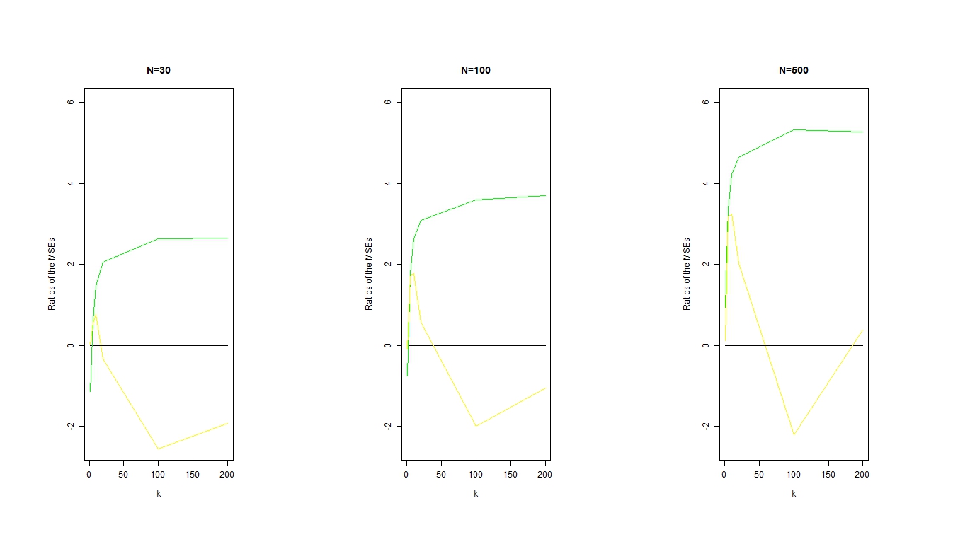
Figure 3: Logarithm of ratio of the MSEs for dependent case (black for $\widehat{M}_{Prod}$, green for $\widehat{M}_{EMP}$, yellow for $\widehat{M}_{\hat{Q}}$).

4.3 Findings from the simulation study

From the simulations we find that our proposed estimator $\widehat{M}_{Prod}$ performs very well for small sample size $n\leq 100$ and small values of $k$ for $F_{E}$ distribution and for large sample size we can consider $\widehat{M}_{ML}$ estimator. For $F_{P}$ distribution our proposed estimator $\widehat{M}_{Prod}$ outperforms other estimators for large sample size $100\leq n$ and for almost all values of $k$ and for small sample it works only when $k=1$ and $5$. We also observe that for $n=30$, $\widehat{M}_{EMP}$ is better for some values of $k$ but far worse for small values of $k$ in the i.i.d case. In the dependent case $\widehat{M}_{Prod}$ is clearly better than all other methods for all sample sizes and small values of $k$ i.e. for 5 and 10 in terms of MSE. When the sample size is large $\widehat{M}_{Prod}$ out performs for all values of $k$ except for $k=100$.

4.4 Coverage probabilities

This section conducts a simulation study, where we estimate the coverage probabilities of confidence intervals that capture the population parameter of interest. We have considered the $F_{E}$ and $F_{P}$ which are defined in section (4.1). For each distribution $F_{E}$ and $F_{P}$, we created 10,000 confidence intervals and each $\widehat{M}_{Prod}^{*}$ has been obtained from 1000 bootstrap replicates. For nominal confidence level $90\%$ we have obtained coverage probabilities with $n=30$, $100$, $500$ and $k=1$, $5$, $10$, $20$, $100$ and $200$. The results are reported in Table 4. From Table 4 we observe that for higher values of $k$ the coverage probabilities are too low. However, for small values of $k$ the coverage probabilities are close to the nominal confidence level $90\%$.

Table 4: Simulated coverage probabilities of the bootstrap confidence intervals for $F_{E}$ and $F_{P}$ distribution.

Distribution	$k$	30	100	500
		$n$
$F_{E}$	1	0.872	0.89	0.92
	5	0.86	0.871	0.911
	10	0.85	0.86	0.901
	20	0.82	0.84	0.891
	100	0.79	0.83	0.89
	200	0.77	0.80	0.85
$F_{P}$	1	0.88	0.89	0.91
	5	0.85	0.872	0.89
	10	0.821	0.832	0.876
	20	0.8	0.82	0.85
	100	0.75	0.777	0.80
	200	0.73	0.74	0.78

5 Data analysis

To illustrate our work we use the thoroughly researched Norwegian fire claims data (see [Nadarajah and Bakar(2015)], [Brazauskas and Kleefeld(2016)] and [Upretee(2020)]) available in the “CASdatasets” package in R software. The Norwegian fire claims data show the overall amount of harm caused by fires in Norway from 1972 to 1992. It’s worth noting that only damages in excess of $500,000$ Norwegian krones (NOK) are covered. It’s also unclear whether the claims were adjusted for inflation. Table 5 summarizes the data sets over the last $12$ years, from $1981$ to $1992$. The table shows that these data sets contain all of the standard characteristics of insurance claims. From Table 5 we observe that the majority of frequently occurring claims are rather small, but as severity increases, claim frequency decreases and a small fraction of extremely big claims occur.

We analyze the data sets for the final $12$ years, $1981$-$1992$, to compare our findings with that of [Upretee(2020)] and [Brazauskas and Kleefeld(2016)]. Due to the fact that no information is provided below $500,000$ and there is no policy limitation, the random variable that generated the data is left truncated at $d=500,000$ but is not censored. The exponential SRM is calculated based on our simulation studies using the $\widehat{M}_{Prod}$ estimator. In Table 6 we report the point estimates and $90\%$ confidence intervals of exponential SRM using PL estimator for Norwegian Fire Claims data. We run $10,000$ simulated samples. In each iteration a random sample of size 100 is selected with replacement from the data. Using each sample, the lower and upper limits of the confidence interval are calculated. Examining the SRM values reveals several patterns in Table 6. We notice that the riskiness of Norwegian fire claims does not show any discernible trend over time, neither higher nor decrease, as seen in [Brazauskas and Kleefeld(2016)]. From Table 6 we also observe that the length of confidence intervals are different through out all the years, for the year 1982 we observe that when $k$ values are small it’s narrower compared to higher values. Whereas for the year 1981 the length of the interval is almost equal for all values of $k$. We even observe that our SRM estimates have much narrower confidence intervals as compared to the VaR and ES estimates of [Upretee(2020)]. Hence we can say that our SRM estimator is much more precise.

We consider a more recent data set i.e. Spain automobile insurance claims (see [Guillen et al.(2021)]). The data represents the claims in the motor insurance policy in Spain for the years 2010 through 2014. It’s worth noting that only damages in excess of 0.72 Euros are covered. Only the claims at fault are considered. Table 7 summarizes the data sets, from 2010 to 2014. From Table 7 similar observations can be observed where the most frequent claims are relatively small and a tiny number of extremely large claims. Since no information is available below $d=0.72$ and there do not exist any policy limitation, the random variable that generated data is left truncated at $d=0.72$ but not censored. In Table 8 we report the point estimates and $90\%$ confidence intervals of exponential SRM for Spain automobile insurance claims. We calculate the confidence intervals in the same way we calculate the confidence for the Norwegian fire claim data. We note that there is no obvious upward or downward trend in the riskiness of auto insurance claims over time. Table 8 shows that the length of the confidence intervals are different for all the years, it is difficult to point out exactly under which value of $k$ the interval is consistently narrower and wider.

To illustrate our work we also use the French marine losses data available in the “CASdatasets” package in R software. The data set comprises of $1,274$ marine losses between $2003$ and $2006$. It’s worth noting that damages lying between $0.018$ and $31904.2$ Euros are covered. Table 9 summarizes the data sets, from $2003$ to $2006$. The table shows that these data sets contain all of the standard characteristics of insurance claims. We observe that the most frequent claims are relatively small however, there is a limited fraction of very high claims and claim frequency reduces as severity increases. The random variable that generated data is left truncated and right censored at $d=0.018$ and $u=31904.2$. In Table 10 we report the point estimates and $90\%$ confidence intervals of exponential SRM for French marine losses. We calculate the confidence intervals same as before. We note that neither a higher nor a lower trend can be seen in the riskiness of French marine losses over time. From Table 10 we observe that the confidence intervals are much wider for small values $k$ and much narrow for higher values of $k$.

Table 5: Summary statistics for the Norwegian Fire Claims ($1981$-$1992$) data.

Claim severity (in 1000,000’s)	$1981$	$1982$	$1983$	$1984$	$1985$	$1986$	$1987$	$1988$	$1989$	$1990$	$1991$	$1992$
[$0.5\ 1.0$)	$54.5$	$54.7$	$53.8$	$48.3$	$49.6$	$50.7$	$41.9$	$41.2$	$41.9$	$40.4$	$43.3$	$45.5$
[$1.0\ 2.0$)	$23.5$	$23.8$	$27.8$	$29.8$	$29.2$	$31.2$	$34.7$	$32.8$	$33.3$	$39.0$	$34.0$	$31.4$
[$2.0\ 5.0$)	$13.5$	$14.3$	$12.0$	$15.4$	$14.0$	$11.9$	$17.1$	$16.9$	$18.0$	$16.2$	$17.9$	$16.4$
[$5.0\ 10.0$)	$4.4$	$4.7$	$3.4$	$4.8$	$4.0$	$3.2$	$4.2$	$5.2$	$3.9$	$1.9$	$3.2$	$4.1$
[$10.0\ 20.0$)	$2.3$	$2.1$	$2.2$	$1.1$	$1.6$	$1.7$	$1.2$	$1.9$	$1.9$	$1.4$	$1.3$	$1.6$
[$20.0\ \infty$)	$1.6$	$0.5$	$0.7$	$0.5$	$1.6$	$1.2$	$1.0$	$1.9$	$1.0$	$1.0$	$0.3$	$1.0$
Top three claims	$43$	$19$	$22$	$22$	$60$	$87$	$35$	$84$	$45$	$26$	$17$	$45$
	$62$	$20$	$30$	$56$	$70$	$98$	$38$	$151$	$86$	$41$	$35$	$50$
	$78$	$23$	$51$	$106$	$135$	$188$	$45$	$465$	$145$	$79$	$50$	$102$
Sample size	$429$	$428$	$407$	$557$	$607$	$647$	$767$	$827$	$718$	$628$	$624$	$615$

• Notes: Relative frequencies are in $\%$.

Table 6: Point and interval estimates of exponential SRM for Norwegian Fire Claims data using $\widehat{M}_{Prod}$ estimator (measured in 1000 millions NOK).

Year	$1$	$5$	$10$	$20$	$100$	$200$
	$k$
$1981$	$4.218$	$13.521$	$22.690$	$39.017$	$192.475$	$384.950$
	[3.718 4.718]	[13.053 13.989]	[22.202 23.178]	[38.583 39.451]	[191.978 192.973]	[384.479 385.421]
$1982$	$4.508$	$9.611$	$16.430$	$28.253$	$139.375$	$278.750$
	[4.299 4.716]	[9.398 9.824]	[16.227 16.633]	[28.031 28.475]	[139.150 139.600]	[278.536 278.964]
$1983$	$3.705$	$10.628$	$16.809$	$28.904$	$142.588$	$285.175$
	[3.356 4.054]	[10.319 10.936]	[16.508 17.110]	[28.609 29.199]	[142.272 142.904]	[284.874 285.476]
$1984$	$3.196$	$8.951$	$13.059$	$22.456$	$110.775$	$221.550$
	[2.813 3.578]	[8.575 9.326]	[12.680 13.437]	[22.087 22.825]	[110.418 111.132]	[221.263 221.837]
$1985$	$3.518$	$12.406$	$24.632$	$42.357$	$208.950$	$417.900$
	[3.003 4.032]	[11.908 12.903]	[24.076 25.187]	[41.886 42.828]	[208.472 209.428]	[417.414 418.386]
$1986$	$3.443$	$15.314$	$20.024$	$34.433$	$169.863$	339.725
	[2.909 3.976]	[14.638 15.989]	[19.472 20.575]	[33.849 35.017]	[169.177 170.549]	[339.089 340.362]
$1987$	$3.566$	$9.844$	$17.136$	$29.467$	$145.363$	290.725
	[3.361 3.770]	[9.627 10.060]	[16.925 17.347]	[29.242 29.692]	[145.139 145.587]	[290.486 290.965]
$1988$	$4.579$	$14.010$	$21.635$	$45.656$	$225.225$	$450.450$
	[3.516 5.641]	[12.845 15.176]	[20.622 22.648]	[44.701 46.611]	[224.109 226.341]	[449.520 451.380]
$1989$	$3.997$	$9.947$	$26.551$	$37.203$	$183.525$	367.050
	[3.588 4.405]	[9.585 10.309]	[26.203 26.899]	[36.832 37.574]	[183.162 183.888]	[366.696 397.404]
$1990$	$3.335$	$7.511$	$16.261$	$27.962$	$137.938$	275.875
	[3.056 3.614]	[7.232 7.790]	[15.982 16.540]	[27.683 28.241]	[137.659 138.217]	[275.596 276.154]
$1991$	$3.128$	$8.337$	$12.572$	$21.619$	$106.650$	213.300
	[2.929 3.327]	[8.138 8.576]	[12.373 12.771]	[21.421 21.818]	[106.451 106.840]	[213.101 213.499]
$1992$	$3.568$	$10.052$	$16.639$	$28.613$	$141.150$	282.300
	[3.210 3.935]	[9.685 10.419]	[16.272 17.006]	[28.246 28.979]	[140.783 141.517]	[281.933 282.666]

Table 7: Summary statistics for the Motor Claims of Spain ($2010$-$2014$) data.

Claim (in 1000)	$2010$	$2011$	$2012$	$2013$	$2014$
[$0.00072\ 1.0$)	$75.03$	$75.86$	$72.33$	$71.77$	$77.42$
[$1.0\ 20.0$)	$24.83$	$23.58$	$26.73$	$28.3$	$22.58$
[$20.0\ \infty$)	$0.13$	$0.55$	$0.94$	$0$	$0$
Top three claims	$16$	$26$	$28$	$13$	$6$
	$17$	$28$	$48$	$14$	$6$
	$20$	$91$	$110$	$14$	$9$
Sample size	$769$	$547$	$318$	$209$	$124$

• Notes: Relative frequencies are in $\%$.

Table 8: Point and interval estimates of exponential SRM for Motor Claims of Spain data using $\widehat{M}_{Prod}$ estimator (measured in 1000 Euros).

$k$	$2010$	$2011$	$2012$	$2013$	$2014$
$1$	$2.220$	$1.924$	$2.346$	$2.323$	$1.773$
	[2.085 2.354]	[1.614 2.234]	[1.809 2.883]	[2.080 2.566]	[1.594 1.954]
$5$	$5.516$	$4.724$	$5.417$	$5.087$	$3.385$
	[5.380 5.652]	[4.354 5.094]	[4.778 6.056]	[4.827 5.347]	[3.221 3.549]
$10$	$7.213$	$6.177$	$7.083$	$6.651$	$4.427$
	[7.080 7.346]	[5.855 6.499]	[6.545 7.621]	[6.389 6.913]	[4.250 4.604]
$20$	$12.403$	$10.623$	$12.179$	$11.438$	$7.612$
	[12.269 12.537]	[10.358 10.888]	[11.587 12.771]	[11.179 11.697]	[7.434 7.790]
$100$	$61.186$	$52.402$	$60.082$	$56.424$	$37.550$
	[61.058 61.314]	[52.149 52.655]	[59.529 60.635]	[56.167 56.681]	[37.366 37.734]
$200$	$122.372$	$104.804$	$120.164$	$112.848$	$75.100$
	[122.235 122.509]	[104.427 105.181]	[119.434 120.895]	[112.619 113.077]	[74.924 75.276]

Table 9: Summary statistics for French marine losses ($2003$-$2006$) data.

Claim (in 100)	$2003$	$2004$	$2005$	$2006$
[$0.00018\ 0.1$)	$72.81$	$72.04$	$72.15$	$79.12$
[$0.1\ 1$)	$22.36$	$24.19$	$25.63$	$20.88$
[$1\ 319.042$)	$4.83$	$3.76$	$2.22$	$0$
Top three claims	$61$	$11$	$1.574$	$0.413$
	$12$	$13$	$1.898$	$0.503$
	$19$	$37$	$2.117$	$0.75$
Sample size	$331$	$372$	$316$	$91$

• Notes: Relative frequencies are in $\%$.

Table 10: Point and interval estimates of exponential SRM for French marine losses using $\widehat{M}_{Prod}$ estimator (measured in Euros).

$k$	$2003$	$2004$	$2005$	$2006$
$1$	$53.1106$	$193.7764$	$6.4237$	$36.3102$
	[39.7069 66.513]	[179.1692 208.3836]	[4.2027 8.6447]	[34.3744 38.2459]
$5$	$100.7767$	$464.3075$	$9.8698$	$84.0595$
	[87.3763 114.1771]	[447.18 481.435]	[7.6498 12.0898]	[82.1118 86.0072]
$10$	$147.0959$	$711.0137$	$14.1909$	$128.0116$
	[134.2763 159.9155]	[692.5611 729.4663]	[11.7036 16.6782]	[126.0887 129.9345]
$20$	$255.9011$	$1264.098$	$25.2578$	$227.5283$
	[243.5670 268.2352]	[1246.429 1281.767]	[22.9568 27.5588]	[225.6388 229.4178]
$100$	$1262.5$	$6250$	$125$	$1125$
	[1248.532 1276.468]	[6234.653 6265.347]	[122.599 127.401]	[1123.004 1127.996]
$200$	$2525$	$12500$	$250$	$2250$
	[2512.178 2537.822]	[12483.34 12516.66]	[247.5354 252.4646]	[2248.107 2251.893]

6 Conclusion remarks

LTRC data are common when we are dealing with insurance data and because of truncation and censoring the actual sample size is always unknown. In this scenario the estimation of an appropriate risk measure becomes critical and and to solve such problem the first task is to find point estimates of the risk measure and assess their variability. In this paper we have discussed about the SRMs, which is a coherent risk measure and the estimation of SRMs for the LTRC data. As mentioned in the introduction when dealing with LTRC data the best choice is to use the PL estimator. Hence based on the PL estimator we proposed an estimator of SRM called $\widehat{M}_{Prod}$ and derived the asymptotic normality for i.i.d case. The $U$-statistic representations of $\widehat{M}_{Prod}$ has been established and used to derive the Edgeworth expansion of $\widehat{M}_{Prod}$. Next we use the Efron’s bootstrap method to approximate the distribution of $\widehat{M}_{Prod}$ and showed that the distribution approximates to its true distribution with an error term $o(n^{-1/2})$. This means that the coverage error for the bootstrap confidence interval is $o(n^{-1/2})$.

In the simulation study we have compared our proposed estimator $\widehat{M}_{Prod}$ with the existing parametric and non parametric estimators such as $\widehat{M}_{EMP}$, $\widehat{M}_{\hat{Q}}$, $\widehat{M}_{ML}$ and $\widehat{M}_{PM}$. Also, we have considered both i.i.d and dependent model in the simulation study. From our study we observe that our proposed estimator $\widehat{M}_{Prod}$ is a suitable estimator of SRM when we are dealing with LTRC data and the observations are both i.i.d. and dependent. We even observe that the choice of $k$ plays an important role in estimating SRM. We observe that for small values of $k$ i.e. for 5, 10 and for small sample size $n\leq 100$, our proposed $\widehat{M}_{Prod}$ estimator is the best choice in case of i.i.d and in dependent case for all sample sizes and for $k=5,\ 10$, it is the best choice. We also observe that the coverage probabilities obtained through simulations are close to the nominal confidence level $90\%$ when $k$ is higher. Based on our simulation study we estimate the exponential SRM of three data sets viz: two left truncated i.e. Norwegian fire claims and Spain automobile insurance claims and one LTRC data set French marine loss. We observe that the riskiness of all three data sets does not exhibit any obvious trend, neither upward nor downward. We even observe that our SRM estimates for Norwegian fire claims have much narrower confidence intervals as compared to the VaR and ES estimates of [Upretee(2020)]. So, we can say that our SRM estimator is much more precise than the estimators considered in [Upretee(2020)].

Disclosure statement: The authors have no conflicts of interest to declare.

Funding:This research is funded by the Department of Science and Technology, India and the grant number is SR/WOS-A/PM-37/2019.

Appendix A Some Definitions

Definition 2

([Delbaen(2002)]) Let, $\psi$ denote the real valued random variables on a probability space ($\Omega,\ \mathcal{F},\ \mathbb{P}$). A coherent risk measure is a function $\rho:\psi\rightarrow\mathbb{R}$ satisfying the following properties:

1. $X\geq 0\Rightarrow\rho(X)\leq 0$.

2. $X\geq Y\Rightarrow\rho(X)\leq\rho(Y),\ X,Y\in\psi.$

3. $\rho(\lambda X)=\lambda\rho(X)$, $\forall\lambda\geq 0,\ X\in\psi.$

4. $\rho(X+k)=\rho(X)-k$, $\forall k\in\mathbb{R},\ X\in\psi.$

5. $\rho(X+Y)\leq\rho(X)+\rho(Y)$, $\forall X,\ Y\in\psi$.

Definition 3

Let, $X\in\psi$ and $F$ be the distribution function of $X$ then $Q_{p}=\inf\{x:F(x)\geq p\},\ 0<p<1$ is the quantile function.

Definition 4

([Gzyl and Mayoral(2008)]) An element $\phi\in\mathcal{L}^{1}([0,1])$ is called an admissible risk spectrum if

1. $\phi\geq 0$

2. $\int_{0}^{1}|\phi(t)|dt=1$

3. $\phi$ is non-decreasing.

Appendix B Some Theorems and Lemmas used in the proof of results discussed in section 3

Theorem 5

[Zhou(1996)] Suppose that assumptions 1 and 2 are satisfied. Then we have uniformly in $a_{W}\leq x\leq b<b_{W}$,

$$\widehat{F}(x)-F(x)=(1-F(x))L_{n}(x)+R_{n2}(x)$$

with

$$\sup_{a_{W}\leq x\leq b}|R_{n2}(x)|=O(n^{-1}\log\log n)\ a.s.$$ (13)

where

$$L_{n}(x)=\int_{a_{W}}^{x}\frac{d(W_{n}^{*}(y)-W^{*}(y))}{C(y)}-\int_{a_{W}}^{x}\frac{C_{n}(y)-C(y)}{C^{2}(y)}dW^{*}(y).$$

The next result follows from [Gurler et al.(1993)] that if $a_{W}<F^{-1}(t_{1})\leq F^{-1}(t_{2})<b_{W}$, $F$ has a continuous and positive density $f$ on [$F^{-1}(t_{1})-\beta$, $F^{-1}(t_{2})+\beta$] for some $\beta>0$ then as $n\rightarrow\infty$,

$$\sup_{t_{1}\leq t\leq t_{2}}\Big{|}\widehat{F}^{-1}(t)-F^{-1}(t)-\frac{t-\hat{F}(F^{-1}(t))}{f(F^{-1}(t))}\Big{|}=o_{p}(n^{-1/2})$$ (14)

Next theorem, gives the $U$-statistic representation for the PL estimator $\widehat{F}$ with sufficiently small remainder term.

Theorem 6

([Wang and Jing(2006)]) Suppose $F$ is a continuous df and $a_{G}<a_{W}$. Then, for any fixed $x$ such that $a_{W}\leq x\leq b<b_{W}$, we have

$$\widehat{F}(x)-F(x)=(1-F(x))U^{(n)}-\frac{(1-F(x))\sigma_{0}^{2}}{2n}+\alpha_{n},$$

with $P(\sqrt{n}|\alpha_{n}|>cn^{-1/2}\log^{(-1)}{n})=o(n^{-1/2})$.

Lemma 2

([Wang and Jing(2006)]) Let, $\sigma_{n}^{2}$ be the variance of $U^{(n)}$. Then, under the conditions of Theorem 6, for any $a_{W}\leq x\leq b<b_{W}$, we have

$$\sup_{y}|P(\sqrt{n}\sigma_{n}^{-1}U^{(n)}\leq y)-E_{n0}(y)|=o(n^{-1/2}),$$

where

$$E_{n0}(y)=\Phi(y)-\frac{\kappa_{3}}{6}n^{-1/2}\phi_{1}(y)(y^{2}-1),$$

$$\kappa_{3}=\frac{1}{\sigma_{0}^{3}}\Big{(}-\frac{15}{2}\sigma_{0}^{4}+\int_{a_{W}}^{x}\frac{dW^{*}(t)}{C^{3}(t)}\Big{)}.$$

Lemma 3

([Wang and Jing(2006)]) For any bounded function $H(y)$, there exists a constant $\alpha$ such that for any random variables $X^{0}$, $Y^{0}$, and constant $a>0$

$$\sup_{y}|P(X^{0}+Y^{0}\leq y)-H(y)|\leq\sup_{y}|P(X^{0}\leq y)-H(y)|+\alpha a+P(|Y^{0}|\geq a).$$

Appendix C Proofs of results in section 3

Proof of Theorem 1:

$$\widehat{M}_{Prod}-M_{\phi} = \int_{0}^{1}(\widehat{F}^{-1}(u)-F^{-1}(u))\phi(u)du.$$ (15)

Let, $a_{W}<F^{-1}(u_{1})\leq F^{-1}(u_{2})<b_{W}$ and using equation (14) and theorem 5 we have

$$\widehat{F}^{-1}(u)-F^{-1}(u) = -\frac{\widehat{F}(F^{-1}(u))-F(F^{-1}(u))}{f(F^{-1}(u))}$$

$$= \frac{-1}{f(F^{-1}(u))}\Big{[}(1-F(F^{-1}(u)))\Big{(}\int_{a_{W}}^{F^{-1}(u)}\frac{d(W_{n}^{*}(y)-W^{*}(y))}{C(y)}-\int_{a_{W}}^{F^{-1}(u)}\frac{C_{n}(y)-C(y)}{C^{2}(y)}dW^{*}(y)\Big{)}\Big{]}$$

$$= \frac{-1}{f(F^{-1}(u))}\Big{[}(1-u)\Big{(}\frac{1}{n}\sum_{i=1}^{n}\frac{I(Y_{i}\leq F^{-1}(u),\delta_{i}=1)}{C(Y_{i})}-\int_{a_{W}}^{F^{-1}(u)}\frac{1/n\sum_{i=1}^{n}I(T_{i}\leq y\leq Y_{i})}{C^{2}(y)}dW^{*}(y)\Big{)}\Big{]}$$

$$= \frac{-(1-u)}{nf(F^{-1}(u))}\sum_{i=1}^{n}\Big{[}\frac{I(Y_{i}\leq F^{-1}(u),\delta_{i}=1)}{C(Y_{i})}-\int_{a_{W}}^{F^{-1}(u)}\frac{I(T_{i}\leq y\leq Y_{i})}{C^{2}(y)}dW^{*}(y)\Big{]}$$

Now we can write

$$\widehat{M}_{Prod}-M_{\phi} = \frac{1}{n}\sum_{i=1}^{n}\int_{0}^{1}\frac{-(1-u)}{f(F^{-1}(u))}\Big{[}\frac{I(Y_{i}\leq F^{-1}(u),\delta_{i}=1)}{C(Y_{i})}-\int_{a_{W}}^{F^{-1}(u)}\frac{I(T_{i}\leq y\leq Y_{i})}{C^{2}(y)}dW^{*}(y)\Big{]}\phi(u)du$$

Let,

$$T_{i}=\int_{0}^{1}\frac{-(1-u)}{f(F^{-1}(u))}\Big{[}\frac{I(Y_{i}\leq F^{-1}(u),\delta_{i}=1)}{C(Y_{i})}-\int_{a_{W}}^{F^{-1}(u)}\frac{I(T_{i}\leq y\leq Y_{i})}{C^{2}(y)}dW^{*}(y)\Big{]}\phi(u)du.$$

$$E(T_{i}) = E\Big{[}\int_{0}^{1}\frac{-(1-u)}{f(F^{-1}(u))}\Big{[}\frac{I(Y_{i}\leq F^{-1}(u),\delta_{i}=1)}{C(Y_{i})}-\int_{a_{W}}^{F^{-1}(u)}\frac{I(T_{i}\leq y\leq Y_{i})}{C^{2}(y)}dW^{*}(y)\Big{]}\phi(u)du\Big{]}$$

$$= \int_{0}^{1}\frac{-(1-u)}{f(F^{-1}(u))}E\Big{[}\frac{I(Y_{i}\leq F^{-1}(u),\delta_{i}=1)}{C(Y_{i})}-\int_{a_{W}}^{F^{-1}(u)}\frac{I(T_{i}\leq y\leq Y_{i})}{C^{2}(y)}dW^{*}(y)\Big{]}\phi(u)du$$

$$= \int_{0}^{1}\frac{-(1-u)}{f(F^{-1}(u))}\Big{[}\frac{P(T\leq F^{-1}(u),\delta=1|T\leq Y)}{C(Y)}-\int_{a_{W}}^{F^{-1}(u)}E\Big{(}\frac{I(T_{i}\leq y\leq Y_{i})}{C^{2}(y)}\Big{)}dW^{*}(y)\Big{]}\phi(u)du$$

$$= \int_{0}^{1}\frac{-(1-u)}{f(F^{-1}(u))}\Big{[}P(T\leq F^{-1}(u),\delta=1|T\leq Y)-\int_{a_{W}}^{F^{-1}(u)}\frac{P(T\leq y\leq Y|T\leq Y)}{C^{2}(y)}dW^{*}(y)\Big{]}\phi(u)du$$

$$= \int_{0}^{1}\frac{-(1-u)}{f(F^{-1}(u))}\Big{[}P(T\leq F^{-1}(u),\delta=1|T\leq Y)-\int_{a_{W}}^{F^{-1}(u)}\frac{P(T\leq y\leq Y|T\leq Y)}{C^{2}(y)}dW^{*}(y)\Big{]}\phi(u)du$$

$$= \int_{0}^{1}\frac{-(1-u)}{f(F^{-1}(u))}\Big{[}P(T\leq F^{-1}(u),\delta=1|T\leq Y)-\int_{a_{W}}^{F^{-1}(u)}\frac{dW^{*}(y)}{C(y)}\Big{]}\phi(u)du$$

$$= \int_{0}^{1}\frac{-(1-u)}{f(F^{-1}(u))}\Big{[}P(T\leq F^{-1}(u),\delta=1|T\leq Y)-\frac{W^{*}(F^{-1}(u))}{C(Y)}\Big{]}\phi(u)du$$

$$= \int_{0}^{1}\frac{-(1-u)}{f(F^{-1}(u))}[P(T\leq F^{-1}(u),\delta=1|T\leq Y)-P(T\leq F^{-1}(u),\delta=1|T\leq Y)]\phi(u)du$$

$$= 0$$

Therefore,

$$E\Big{[}\frac{1}{n}\sum_{i=1}^{n}T_{i}\Big{]}=0.$$

and

$$\sigma^{2}=V\Big{[}\frac{1}{n}\sum_{i=1}^{n}T_{i}\Big{]}=\int_{0}^{1}\int_{0}^{1}\frac{(1-u)(1-v)}{f(F^{-1}(u))f(F^{-1}(v))}\Big{[}\int_{a_{W}}^{F^{-1}(u)}\frac{dW^{*}(y)}{C^{2}(y)}\int_{a_{W}}^{F^{-1}(v)}\frac{dW^{*}(y)}{C^{2}(y)}-uv\Big{]}\phi(u)\phi(v)dudv.$$

Now an application of Liapunov’s form of the Central Limit Theorem we get

$$\sqrt{n}(Prod-\mu)\xrightarrow{\text{d}}N(0,\sigma^{2})\ as\ n\rightarrow\infty.$$

Proof of Theorem 2: We can write

$$\widehat{M}_{Prod}-M_{\phi} = \int_{0}^{1}(\widehat{F}^{-1}(u)-F^{-1}(u))\phi(u)du.$$

Let, $a_{W}<F^{-1}(u_{1})\leq F^{-1}(u_{2})<b_{W}$ and using equation (14) and theorem 6 we have

$$\widehat{F}^{-1}(u)-F^{-1}(u) = -\frac{\widehat{F}(F^{-1}(u))-F(F^{-1}(u))}{f(F^{-1}(u))}$$

$$= \frac{-1}{f(F^{-1}(u))}\Big{[}(1-F(F^{-1}(u)))\Big{\{}\frac{1}{n^{2}}\sum_{i<j}h_{1}(V_{i};\ V_{j};\ F^{-1}(u))-\frac{1}{2n}\int_{a_{W}}^{F^{-1}(u)}\frac{dW^{*}(x)}{C^{2}(x)}\Big{\}}\Big{]}+\alpha_{n}$$

Now,

$$\int_{0}^{1}(\widehat{F}^{-1}(u)-F^{-1}(u))\phi(u)du = \int_{0}^{1}\frac{-1}{f(F^{-1}(u))}\Big{[}(1-u)\Big{\{}\frac{1}{n^{2}}\sum_{i<j}h_{1}(V_{i};V_{j};F^{-1}(u))-\frac{1}{2n}\int_{a_{W}}^{F^{-1}(u)}\frac{dW^{*}(x)}{C^{2}(x)}\Big{\}}\Big{]}$$

$$\phi(u)du+\alpha_{n}.$$

Proof of Theorem 3:

$$\widehat{M}_{Prod}-M_{\phi} = \int_{0}^{1}(\widehat{F}^{-1}(u)-F^{-1}(u))\phi(u)du.$$

Let, $a_{W}<F^{-1}(u_{1})\leq F^{-1}(u_{2})<b_{W}$ and using equation (14) and theorem 6 we have

$$\widehat{F}^{-1}(u)-F^{-1}(u) = -\frac{\widehat{F}(F^{-1}(u))-F(F^{-1}(u))}{f(F^{-1}(u))}$$

$$= \frac{-1}{f(F^{-1}(u))}\Big{[}(1-F(F^{-1}(u)))\Big{\{}\frac{1}{n^{2}}\sum_{i<j}h_{1}(V_{i};\ V_{j};\ F^{-1}(u))-\frac{1}{2n}\int_{a_{W}}^{F^{-1}(u)}\frac{dW^{*}(x)}{C^{2}(x)}\Big{\}}\Big{]}$$

Now,

$$\int_{0}^{1}(\widehat{F}^{-1}(u)-F^{-1}(u))\phi(u)du = \int_{0}^{1}\frac{-1}{f(F^{-1}(u))}\Big{[}(1-u)\Big{\{}\frac{1}{n^{2}}\sum_{i<j}h_{1}(V_{i};V_{j};F^{-1}(u))-\frac{1}{2n}\int_{a_{W}}^{F^{-1}(u)}\frac{dW^{*}(x)}{C^{2}(x)}\Big{\}}\Big{]}$$

$$\phi(u)du$$

$$= S_{1}+S_{2}$$

where

$$S_{1}=-\int_{0}^{1}\frac{(1-u)}{n^{2}f(F^{-1}(u))}\sum_{i<j}h_{1}(V_{i};\ V_{j};\ F^{-1}(u))\phi(u)du\ \text{and}\ S_{2}=\int_{0}^{1}\frac{(1-u)}{2nf(F^{-1}(u))}\int_{a_{W}}^{F^{-1}(u)}\frac{dW^{*}(x)}{C^{2}(x)}\phi(u)du.$$

We can write

$$\sup_{y}|P(\sqrt{n}\sigma^{-1}(\widehat{M}_{Prod}-M_{\phi})\leq y)-E_{n2}(y)|$$

$$=\sup_{y}|P(\sqrt{n}\sigma^{-1}S_{1}\leq y-\sqrt{n}\sigma^{-1}S_{2})-E_{n2}(y)|$$

$$=\sup_{y}|P(\sqrt{n}\sigma^{-1}S_{1}\leq y)-E_{n1}(y)|+\sup_{y}|E_{n1}(y-\sqrt{n}\sigma^{-1}S_{2})-E_{n2}(y)|$$

$$=\sup_{y}|P(\sqrt{n}\sigma_{01}^{-1}S_{1}\leq y)-E_{n1}(y)|+\sup_{y}|E_{n1}(y-\sqrt{n}\sigma_{01}^{-1}S_{2})-E_{n2}(y)|$$

$$=A+B$$

Now, using Lemma 1 we can say that $A$ is $o(n^{-1/2})$. Clearly,

$$B = \sup_{y}|E_{n1}(y-\sqrt{n}\sigma_{01}^{-1}S_{2})-E_{n2}(y)|$$

$$= \sup_{y}\Big{|}E_{n1}(y)-\Big{[}\frac{d}{dy}E_{n1}(y)\Big{]}\frac{1}{2\sqrt{n}}\sigma_{01}^{-1}\int_{0}^{1}\frac{(1-u)}{f(F^{-1}(u))}\int_{a_{W}}^{F^{-1}(u)}\frac{dW^{*}(x)}{C^{2}(x)}\phi(u)du-E_{n2}(y)\Big{|}+o(n^{-1/2})$$

$$= o(n^{-1/2}),$$

which completes the proof.

Proof of Theorem 4: Similar to Theorem (2), we have

$$\widehat{M}_{Prod}^{*}-M_{Prod}=S^{*}+\alpha_{n}^{*},$$ (16)

where

$$S=-\int_{0}^{1}\frac{1}{f(F^{-1}(u))}\Big{[}\frac{(1-u)}{n^{2}}\sum_{i<j}h_{1}(V_{i};V_{j};F^{-1}(u))-\frac{1-u}{2n}\int_{a_{W}}^{F^{-1}(u)}\frac{dW^{*}(x)}{C^{2}(x)}\Big{]}\phi(u)du$$

and $S^{*}$ and $\alpha_{n}^{*}$ are the bootstrap analogs of $S$ and $\alpha_{n}$. A similar argument to the proof of Lemma 3 in the Appendix of Chen and Lo (1996) yields that

$$\sup_{y}|P(\sqrt{n}T^{*}\leq y)-E_{n1}^{*}(y)|=o(n^{-1/2}),\ a.s.,$$ (17)

where $T=\sigma_{01}^{-1}\frac{1}{n^{2}}\sum_{i<j}h_{1}(V_{i},V_{j};F^{-1}(x))$ and $T^{*}$ and $E_{n1}^{*}(y)$ are the bootstrap analogs of $T$ and $E_{n1}(y)$. Similar to the proof of Theorem (6) (see [Wang and Jing(2006)]), we have with probability 1

$$P(\sqrt{n}|\alpha_{n}^{*}|>cn^{-1/2}\log^{(-1)}{n})=o(n^{-1/2}).$$ (18)

Hence, combining equation (16), (17), and (18) together with Lemma (3) yield

$$\sup_{y}|P(\sqrt{n}\sigma^{-1}(\widehat{M}_{Prod}^{*}-M_{Prod})\leq y)-E_{n2}^{*}(y)|=o(n^{-1/2}),\ a.s.$$

Now, it remains to prove that

$$\sup_{y}|E_{n2}(y)-E_{n2}^{*}(y)|=o(n^{-1/2}),\ a.s.$$ (19)

Notice that

$$\sigma_{01}^{*^{2}}=\int_{a_{W}}^{F^{-1}(x)}\frac{dW^{*^{*}}(t)}{C^{*^{2}}(t)}=\int_{a_{W}}^{F^{-1}(x)}\frac{dW_{n}^{*}(t)}{C_{n}^{2}(t)},\\ \int_{a_{W}}^{F^{-1}(x)}\frac{dW^{*^{*}}(t)}{C^{*^{3}}(t)}=\int_{a_{W}}^{F^{-1}(x)}\frac{dW_{n}^{*}(t)}{C_{n}^{3}(t)}.$$

Hence, $\kappa_{3}^{*}\xrightarrow{\text{p}}\kappa_{3}$. This proves (19). The proof of Theorem (4) is thus complete.

References

• [Acerbi(2002)] Acerbi, Carlo. 2002. “Spectral measures of risk: A coherent representation of subjective risk aversion.” Journal of Banking & Finance 26: 1505–1518.
• [Adam et al.(2008)] Adam, Adam, Mohamed Houkari, and Jean-Paul Laurent. 2008. “Spectral risk measures and portfolio selection.” Journal of Banking & Finance 32: 1870–1882.
• [Artzner et al.(1999)] Artzner, Philippe, Freddy Delbaen, Jean-Marc Eber, and David Heath. 1999. “Coherent measures of risk.” Mathematical Finance 93: 203–228.
• [Brazauskas and Kleefeld(2016)] Brazauskas, Vytaras, and Andreas Kleefeld. 2016. “Modeling severity and measuring tail risk of Norwegian fire claims.” North American Actuarial Journal 20: 1–16.
• [Brazauskas and Upretee(2019)] Brazauskas, Vytaras, and Sahadeb Upretee. 2019. “Model efficiency and uncertainty in quantile estimation of loss severity distributions.” Risks 7: 16 pages, doi:10.3390/risks7020055.
• [Cairns(2000)] Cairns, Andrew J. 2000. “A discussion of parameter and model uncertainty in insurance.” Insurance: Mathematics and Economics 27: 313–330.
• [Calderin-Ojeda et al.(2023)] Calder$\acute{i}$n-Ojeda, Enrique, Emilio G$\acute{o}$mez-D$\acute{e}$niz, and Francisco J. V$\acute{a}$zquez-Polo. 2023. “Conditional tail expectation and premium calculation under asymmetric loss.” Axioms 12: 496.
• [Chang (1991)] Chang, Myron N. 1991. “Edgeworth expansion for the kaplan-meier estimator.” Communications in Statistics-Theory and Methods 20(8): 2479–2494.
• [Cheng et al.(2016)] Cheng, Jung-Yu, Shu-Chun Huang, and Shinn-Jia Tzeng. 2016. “Quantile regression methods for left-truncated and right-censored data.” Journal of Statistical Computation and Simulation 86: 443–459.
• [Cotter and Dowd(2006)] Cotter, John, and Kevin Dowd. 2006. “Extreme spectral risk measures: an application to futures clearinghouse margin requirements.” Journal of Banking & Finance 30: 3469–3485.
• [Delbaen(2002)] Delbaen, Freddy. 2002. “Coherent risk measures on general probability spaces.” In Advances in finance and stochastics, Springer, pp. 1–37.
• [Dowd and Blake(2006)] Dowd, Kevin, and David Blake. 2006. “After VaR:the theory, estimation, and insurance applications of quantile-based risk measures.” The Journal of Risk and Insurance 73: 193–229.
• [Dowd et al.(2008)] Dowd, Kevin, John Cotter, and Ghulam Sorwar. 2008. “Spectral risk measures: properties and limitations.” Journal of Financial Services Research 34: 61–75.
• [Efron (1979)] Efron, B. 1979. “Bootstrap method: another look at the jackknife.” The Annals of Statistics 7(1): 1–26.
• [Ergashev et al.(2016)] Ergashev, Bakhodir, Konstantin Pavlikov, Stan Uryasev, and Evangelos Sekeris. 2016. “Estimation of Truncated Data Samples in Operational Risk Modeling.” Journal of Risk and Insurance 83(3): 613–640.
• [Gijbels and Wang’s(1993)] Gijbels, Ir$\grave{e}$ne, and Jane-Ling Wang. 1993. “Strong representations of the survival function estimator for truncated and censored data with applications.” Journal of Multivariate Analysis 47: 210–229.
• [Gu(1995)] Gu, Minggao. 1995. “Convergence of increments for cumulative hazard function in a mixed censorship-truncation model with application to hazard estimators.” Statistics & Probability Letters 23: 135–139.
• [Guillen et al.(2021)] Guillen, Montserrat, Bolancé, Catalina, Frees, Edward W., and Valdez, Emiliano A. 2021. “Case study data for joint modeling of insurance claims and lapsation.” Data in Brief 39: 107639.
• [Gurler et al.(1993)] G$\ddot{u}$rler, $\ddot{U}$lk$\ddot{u}$, Stute, Winfried, and Wang, Jane-Ling. 1993. “Weak and strong quantile representations for randomly truncated data with applications.” Statistics & Probability Letters 17: 139-148.
• [Gzyl and Mayoral(2008)] Gzyl, Henryk, and Silvia Mayoral. 2008. “On a relationship between distorted and spectral risk measures.” Revista de economía financiera 15: 8–21.
• [Heras et al.(2012)] Heras, Antonio, Beatriz Balb$\acute{a}$s, and Jos$\acute{e}$ Luis Vilar. 2012. “Conditional tail expectation and premium calculation.” ASTIN Bulletin 42:325–342.
• [Kaiser and Brazauskas(2006)] Kaiser, Thomas, and Vytaras Brazauskas. 2006. “Interval estimation of actuarial risk measures.” North American Actuarial Journal 10: 249–68.
• [Klugman et al.(2004)] Klugman, Stuart A., Harry H. Panjer, and Gordon E. Willmot. 2004. Loss Models: From Data to Decisions, 2nd Edition. John Wiley & Sons Inc., Hoboken, New Jersey.
• [Lai and Ying(1991)] Lai, Tze Leung, and Zhiliang Ying. 1991. “Estimating a distribution function with truncated and censored data.” The Annals of Statistics 417–442.
• [Liang et al.(2015)] Liang, Hanying, Deli Li, and Tianxuan Miao. 2015. “Conditional quantile estimation with truncated, censored and dependent data.” Chinese Annals of Mathematics, Series B 36: 969–990.
• [Nadarajah and Bakar(2015)] Nadarajah, S, and S. A. A. Bakar. 2015. “New folded models for the log-transformed norwegian fire claim data.” Communications in Statistics-Theory and Methods 44: 4408–4440.
• [Pichler(2015)] Pichler, Alois. 2015. “Premiums and reserves, adjusted by distortions.” Scandinavian Actuarial Journal 2015(4): 332–351.
• [Shi et al.(2018)] Shi, Jianhua, Huijuan Ma, and Yong Zhou. 2018 “The nonparametric quantile estimation for length-biased and right-censored data.” Statistics & Probability Letters 134: 150–158.
• [Shorack(1972)] Shorack, Galen R. 1972. “Functions of order statistics.” The Annals of Mathematical Statistics 43: 412–427.
• [Stute(1993)] Stute, Winfried. 1993. “Almost sure representations of the product-limit estimator for truncated data.” The Annals of Statistics, 146–156.
• [Sun(1997)] Sun, Liuquan. 1997. “Bandwidth choice for hazard rate estimators from left truncated and right censored data.” Statistics & Probability Letters 36: 101–114.
• [Sun and Zhou(1998)] Sun, Liuquan, and Yong Zhou. 1998. “Sequential confidence bands for densities under truncated and censored data.” Statistics & Probability Letters 40: 31–41.
• [Tsai et al.(1987)] Tsai, Wei-Yann, Nicholas P. Jewell, and Mei-Cheng Wang. 1987. “A note on the product-limit estimator under right censoring and left truncation.” Biometrika 74: 883–886.
• [Tsukahara(2009)] Tsukahara, Hideatsu. 2009. “One-parameter families of distortion risk measures.” Mathematical Finance: An International Journal of Mathematics, Statistics and Financial Economics 19: 691–705.
• [Upretee(2020)] Upretee, Sahadeb. 2020. “Estimating distortion risk measures under truncated and censored data scenarios.” Ph.D. thesis, The University of Wisconsin-Milwaukee.
• [Uzunoḡullari and Wang(1992)] Uzunoḡullari, $\ddot{U}$lk$\ddot{u}$, and Jane-Ling Wang. 1992. “A comparison of hazard rate estimators for left truncated and right censored data.” Biometrika 79: 297–310.
• [Wang(1987)] Wang, Mel Cheng. 1987. “Product limit estimates: a generalized maximum likelihood study.” Communications in Statistics-Theory and Methods 16: 3117–3132.
• [Wang(1996)] Wang, Shaun. 1996. “Premium calculation by transforming the layer premium density.” ASTIN Bulletin 26(1): 71–92.
• [Wang and Young(1998)] Wang, Shaun S., and Virginia R. Young. 1998. “Risk-adjusted credibility premiums using distorted probabilities.” Scandinavian Actuarial Journal 2:143–165.
• [Wang and Jing(2006)] Wang, Qihua, and Bing-Yi Jing. 2006. “Edgeworth expansion and bootstrap approximation for studentized product-limit estimator with truncated and censored data.” Communications in Statistics-Theory and Methods 35:609–623.
• [Woodroofe(1985)] Woodroofe, Michael. 1985. “Estimating a distribution function with truncated data.” The Annals of Statistics 13: 163–177.
• [Zhou(1996)] Zhou, Yong. 1996. “A note on the tjw product-limit estimator for truncated and censored data.” Statistics & Probability Letters 26: 381–387.
• [Zhou et al.(2000)] Zhou, Xian, Liuquan Sun, and Haobo Ren. 2000. “Quantile estimation for left truncated and right censored data.” Statistica Sinica 1217–1229.
• [Zhou and Yip(1999)] Zhou, Yong, and Paul S. F. Yip. 1999. “A strong representation of the product-limit estimator for left truncated and right censored data.” Journal of Multivariate Analysis 69: 261–280.
• [van Zuijlen(1982)] van Zuijlen, Martin C. A. 1982. “Properties of the empirical distribution function for independent non-identically distributed random vectors.” The Annals of Probability 108–123.