Irregular Bloch-Zener oscillations in - lattices
Abstract
When a static electrical field is applied to a two-dimensional (2D) Dirac material, Landau-Zener transition (LZT) and Bloch-Zener oscillations can occur. Employing - lattices as a paradigm for a broad class of 2D Dirac materials, we uncover two phenomena. First, due to the arbitrarily small energy gaps near a Dirac point that make it more likely for LZTs to occur than in other regions of the Brillouin zone, the distribution of differential LZT probability in the momentum space can form a complicated morphological pattern. Second, a change in the LZT morphology as induced by a mutual switching of the two distinct Dirac points can lead to irregular Bloch-Zener oscillations characterized by a non-smooth behavior in the time evolution of the electrical current density associated with the oscillation. These phenomena are due to mixed interference of quantum states in multiple bands modulated by the geometric and dynamic phases. We demonstrate that the adiabatic-impulse model describing Landau-Zener-Stückelberg interferometry can be exploited to calculate the phases, due to the equivalence between the - lattice subject to a constant electrical field and strongly periodically driven two- or three-level systems. The degree of irregularity of Bloch-Zener oscillations can be harnessed by selecting the morphology pattern, which is potentially experimentally realizable.
I Introduction
The Landau-Zener transition (LZT) [1, 2] is a fundamental phenomenon in time-dependent quantum systems. The paradigmatic setting for LZT is a two-level system in which the two energy levels do not cross each other and vary adiabatically with time. When the energy gap between the two levels is sufficiently small, a non-adiabatic transition from one energy level to another can occur - leading to an LZT. The phenomenon of LZT is relevant to quantum information science and technology, because qubits are essentially two-level systems [3, 4, 5]. In addition to quantum systems, LZTs can arise in other physical situations such as optical lattices [6, 7, 8] and electromechanical systems [9, 10]. When a two-level system is periodically driven by an electric field, the transition probability will depend on the phase accumulated by the two energy bands between subsequent crossings, leading to the so-called Landau-Zener-Stückelberg interferometry [11]. In general, interference among the quantum states in different energy bands is determined by two phases: geometric and dynamic, which correspond to the adiabatic and Stokes phases, respectively, in the adiabatic-impulse model [11, 12] underlying the Landau-Zener-Stückelberg interferometry, where the sum of the adiabatic and Stokes phases gives the Stückelberg phase - a concept originated from strongly periodically driven two-level systems. A generalization from the two-level setting is the three-level LZT model [13] with an additional flat band [14, 15].
In solid state physics, Bloch oscillations [16, 17] are a fundamental phenomenon closely related to LZT, which occur when a static electric field is applied to a periodic lattice, leading to a linear increase with time in the electron momentum and generating a time-dependent quantum system. The basic periodicity of the momentum space stipulates that the electron must execute oscillatory motions in the physical space at a frequency determined by the lattice constant and the electric field strength (typically in the terahertz regime). In fact, insofar as the electron moves in a periodic potential, Bloch oscillations can occur, rendering them a common quantum phenomenon beyond a solid-state lattice. In the past, the oscillations have been observed in diverse systems such as semiconductor superlattices [18], photonic structures [19, 20, 21, 22] and plasmonic waveguide arrays [23]. The phenomenon provides a viable way to convert a direct current to a high-frequency signal [24, 25].
Bloch oscillations arise from the time evolution of the electron in a single energy band. When there are multiple energy bands, LZTs can occur at the avoided crossing points between the bands. Driven by the static electric field, a quantum state initialized in the lower energy band evolves with time. At certain time, the state will reach an avoided crossing point between distinct energy bands and possibly experience an LZT. Thus, in systems with multiple energy bands, a combination of LZTs and Bloch oscillations can occur, leading to the so-called Bloch-Zener oscillations [26, 27, 15, 28], which have applications in, e.g., matter-wave beam splitters and Mach-Zender interferometry [29, 30]. In the past, Bloch-Zener oscillations were extensively studied in one-dimensional (1D) gapped periodic lattices [31, 29, 30, 32] and were demonstrated to be sensitive to the size of the energy gap. In particular, if the gap is relatively large, LZTs are inhibited so the Bloch-Zener oscillations are restricted to within a single energy band. For a smaller gap, interband LZTs can occur, which destroys the periodicity of the Bloch-Zener oscillations [31, 29, 30, 33, 34]. In a 2D lattice with multiple energy bands, in the first Brillouin zone, different subregions can arise that can inhibit or excite LZTs, resulting in irregular Bloch-Zener oscillations [35, 36]. For example, in pure graphene, when a constant electric field is applied in a lattice-rational direction, the oscillation amplitude can decay with time rapidly in a non-adiabatic fashion [37]. When the electric field is in an irrational direction with respect to the lattice structure, Bloch oscillations of complicated patterns can arise [38].
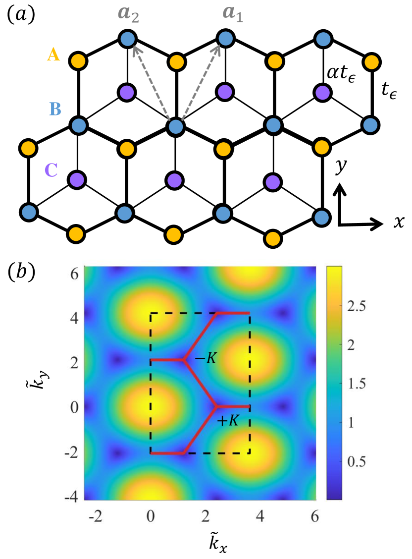
In this paper, we study the effects of a constant and uniform electric field on a broad class of 2D Dirac materials, the - lattice [39, 40], which has an additional atom at the center of each unit cell of the honeycomb graphene lattice. The interaction between the central atom and any of its nearest neighbors is characterized by the parameter - effectively the strength relative to that between two neighboring atoms at the vertices of the graphene cell. For , the lattice reduces to that of graphene with quasiparticles being pseudospin-1/2 Dirac fermions. As increases from zero, a flat band through the conic interaction of the two Dirac cones emerges [39, 40]. The maximal value gives a pseudospin-1 lattice where, because of the extra atom, the low energy excitations need to be described by the pseudospin-1 Dirac-Weyl equation with a three-component spinor [41]. A distinct feature of the entire spectrum of - lattices is the existence of two distinct valleys centered about the two non-equivalent Dirac points of the backbone hexagonal lattice, denoted as and .
Depending on the direction and magnitude of the electric field, electrons initiated from distinct valleys can exhibit characteristically different LZTs. As the dynamic phases associated with different valleys cancel each other exactly, the distinct LZTs are due to the different adiabatic phases of the quantum states in the energy bands between consecutive crossings. This can be understood by considering the reciprocal periodic momentum space with the hexagonal Brillouin zone, as shown in Fig. 1. Now apply an electric field in the direction. The component of the momentum will then increase linearly with time under the premise of the same energy value. As a result, the Dirac points and will shift towards the right. At an original Dirac point (+ or ), the energy will increase from zero, reach a maximum, and then decrease to zero when the next Dirac point arrives, generating a time-periodic behavior. Because of the hexagonal structure of the momentum space, the energy variations associated with and are distinct, as indicated in Fig. 1(b). The LZT probability depends on the accumulated phase between subsequent crossings, where the adiabatic phase is the integral of the energy variation over time. In the specific setting of Figs. 1(a) and 1(b), the integral associated with the Dirac point will have a much larger value than that associated with the other Dirac point . As a result, if an electron initiates with a momentum value near , the adiabatic phase will be nearly constant for a large range of energy gaps determined by the momentum deviation from the trajectory of Dirac points in the direction. However, if an electron starts with a momentum value near , the adiabatic phase will depend sensitively on the energy gap. Based on this property, it is possible to generate specific destructive or constructive interference for a large range of momentum deviation from the trace of the Dirac point , whereas there is mixed interference associated with all possible phases for electrons with initial momentum near .
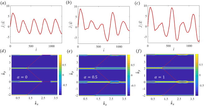
Our first finding is the emergence of complicated LZT morphological patterns in the vicinity of distinct Dirac points, which is associated with mixed quantum interference among the quantum states in multiple bands. Say we apply an electric field in the direction, initialize electrons in the lower Dirac cone (the lower band), and calculate the differential LZT probability, defined as the difference between the probability that an electron is in the upper band and that in the lower band. Different momentum values about a Dirac point and the magnitudes of the electric field give distinct interference phases. As a result, in the momentum plane, the differential LZT probability displays different values, giving rise to some morphological pattern that can be complex. During its temporal evolution, the pattern can be maintained for some time but it can change from time to time due to the switching of two two distinct Dirac points in the Brillouin zone as caused by the external electric field and the periodic structure of the momentum space. Specifically, during one period of the Bloch-Zener oscillation, the two valleys go through a complete cycle in the sense that they are switched and then returned to their respective original positions.
The second finding is that changes in the LZT morphology can lead to irregularities in Bloch-Zener oscillations in - lattice. To explain this, we recall the two typical cases where periodic Bloch oscillations are generated. One case is a single-band material, such as a normal conductor, where the Bloch oscillations are characterized by a perfect temporally periodic behavior in the electrical current density. Another case is where an LZT causes all electrons initialized in one band to transition completely to another band, i.e., the transition probability is one - the so-called ideal LZT. In this case, the resulting Bloch-Zener oscillations behave as if the electrons were in a single band. In the three-band - lattice, LZTs are typically not ideal. The mutual switchings of the two Dirac points in the Brillouin zone changes the LZT morphology, which can produce an abrupt, nonsmooth change in the current density, thereby leading to aperiodic, irregular Bloch-Zener oscillations. More specifically, the coexistence of a variety of LZT possibilities in the momentum space generates complex, mixed quantum interference between the states in the upper, lower, and flat bands, disrupting the originally periodic Bloch-Zener oscillation rhythm before the Dirac point switch. While aperiodic Bloch oscillations [31, 29, 30, 33, 34] and irregular Bloch-Zener oscillations [35, 36] have been noted before, to our knowledge, the physical mechanisms underlying these irregular behaviors were not clear. Especially, it has not been reported previously that LZTs can form a complicated morphology in - lattice and a change in the morphology can lead to irregular Bloch-Zener oscillations.
In Sec. II, we describe the - lattice model and derive the current density associated with the Bloch-Zener oscillations from the adiabatic basis in the hexagonal Brillouin zone. In Sec. III, we present a general treatment of LZTs in the - lattice, display the LZTs morphology in the long time, and analyze the relationship between morphology and irregular Bloch-Zener oscillations. In particular, in Sec. III.1, we linearize the Hamiltonian about the Dirac points to obtain the effective Landau-Zener Hamiltonian for the two limiting cases: and . For , we numerically demonstrate the occurrence of LZT. In Sec. III.2, we elucidate the interplay between LZT morphological changes and irregular Bloch-Zener oscillations. In Sec. IV, we focus on the Landau-Zener-Stückelberg interferometry in - lattice, where in Sec. IV.1, we establish the equivalence of the - lattice to two- or three-level time-dependent systems and provide an understanding of the LZT based on the Stückelberg phase. In Sec. IV.2, we address the problem of harnessing irregular Bloch-Zener oscillations through selection of the LZT morphology and discuss the experimental feasibility of this scheme. A discussion is offered in Sec. V.
II Basics of - lattice, Landau-Zener transition, and Bloch-Zener oscillations
The - lattice interpolates between the graphene honeycomb lattice () and the dice lattice () with the parametrization with the duality [42] . The tight-binding Hamiltonian is given by
| (1) |
where
| (2) |
, and is the nearest-neighbor hopping energy between A and B sites, as shown in Fig. 1(a). The primitive translation vectors are and with being the lattice constant. The corresponding primitive translation vectors in the hexagonal Brillouin zone of the reciprocal lattice are and . The eigenenergy spectrum of the - lattice is independent of , which consists of two conic dispersive bands distinguished by the band index and a zero energy flat band , as shown in Fig. 1(b). The eigenstates of the - lattice in the whole hexagonal Brillouin zone can be obtained through the following effective Hamiltonian about the Dirac points:
| (9) |
where is the angle of associated with the specific momentum.
We describe the Hamiltonian underlying Bloch-Zener oscillations. Apply a uniform and constant electric field to the - lattice in the direction, which is switched on at . With the time-dependent vector potential [44, 45] , where , the Hamiltonian becomes
| (13) |
where is given by
| (14) |
with . For convenience, we define the dimensionless quantities
| (15) | ||||
| (16) |
so that has the same dimension as the hopping energy .
In the presence of the electric field, the eigenenergy spectrum of the positive dispersion band in the whole hexagonal Brillouin zone is determined by
| (17) |
where and . Because the function includes , where is a linear function of time, the Hamiltonian becomes time-periodic. Consider the special case of (graphene). Expanding the Hamiltonian around the Dirac points yields the standard Landau-Zener Hamiltonian [46]:
| (18) |
That is, when the electrons are near the Dirac points, LZTs between distinct energy bands can arise.
The quantum dynamics are governed by
| (19) |
On the adiabatic basis, the evolution of a quantum state is under an infinitesimal electric field [44, 47]:
| (20) |
where is the -component of the vector of spin-1 matrices. The transformed quantum dynamics are governed by
| (21) |
through the time-dependent unitary transformation given by
| (25) |
where and the term incorporating contributes to the time dependence of through . Specifically, we have
| (26) | ||||
| (27) |
where
| (34) |
For , reduces to , the component of spin-1 matrix and Eq. (21) becomes the quantum evolution equation for a dice lattice. This form of Eq. (21) is consistent with that reported in a previous work [45] except for a periodic factor in due to the intrinsic lattice structure. For , become and Eq. (21) describes the graphene lattice, which is consistent with a previous work [44] except for the identity term due to the different form of the basis. Overall, reflects the different coupling strength among the three bands and the periodic term in originates from the intrinsic property of the - lattice.
We set the initial state as one corresponding fully occupied lower band:
| (35) |
The average current density associated with the momentum in the hexagonal Brillouin zone is given by
| (36) |
where the current density matrix with the definite momentum is
| (37) |
and in the adiabatic basis can be written as
| (39) |
Due to the periodic structure of the energy band (referred to as the Bloch band), the average current density will exhibit Bloch oscillations.
The average current density can be decomposed into two components, the intraband and interband currents, respectively [44]:
| (40) |
which can be written as
| (41) | ||||
| (42) |
The matrix provides insights into the current density . In particular, the intraband component consists of both electrons and holes, corresponding to
| (43) | ||||
| (44) |
respectively, where the minus sign comes from the opposite sign of the equivalent charge in the electron-hole pair. The zero group velocity of the flat band results in zero intraband contribution. The interband contribution arises from the interference between the transition from the lower to the flat band or the upper band and that from the flat to the upper band, corresponding to and , respectively, which are given by
| (45) | ||||
| (46) |
where
| (47) |
and is the common factor with the dimension of the current density:
| (48) |
To facilitate numerical calculations, we define the dimensionless quantities:
| (49) | ||||
| (50) | ||||
| (51) | ||||
| (52) |
where , , and . We use the fourth-order Runge–Kutta method to calculate the adiabatic evolution of the particle. The discrete step sizes in time and momentum are chosen according to Eq. (21) with the error tolerance and normalized wavefunction error within . Figure 1(b) indicates that the correspond to zero energy, which results in numerical divergence of Eq. (21), so we set a minimum energy cut-off to be .
The dimensionless current density is the result of integrating over the rectangular reference area in the hexagonal Brillouin zone, as shown in Fig. 1(b), which contains three Dirac points and is times larger than the first Brillouin zone. In addition, we divide the current density by the electric field and a constant , which normalizes the current density in the weak field regime [37] for .
III Morphological changes in LZTs and irregular Bloch-Zener oscillations
III.1 Landau-Zener transition
To gain insights, we first consider the special case (graphene), where the Hamiltonian of the - lattice linearized about the Dirac points corresponds to that of a standard two-level system. Using the unitary transformation
| (53) |
we can write the linearized Hamiltonian as (Appendix C)
| (54) |
where is an infinitesimal deviation from a Dirac point and denotes the starting time from the Dirac point. Recall the standard Landau-Zener Hamiltonian for a two-level system [46]:
| (55) |
with the two underlying adiabatic energy levels
| (56) |
where is the energy gap and is the slope of the two-level band about the LZT point. The linearized Hamiltonian for graphene in Eq. (54) can thus be cast in the standard two-level LZT Hamiltonian with the following parameter correspondences:
| (57) |
For a finite in - lattice, the exact energy gap is
| (58) |
The gap size increases monotonically with the momentum deviation from a Dirac point. [For (a flat band), the gap between the lower band and the flat one is half of the gap between the lower and the upper bands.] For , the gap size reaches the maximum value of two in the energy unit in the hexagonal Brillouin zone.
In a two-level quantum system, for electrons initialized in the lower band, after the electric field is turned on, the first LZT to the upper band occurs with the probability [46]
| (59) |
and the one remaining in the lower band is , where is the ratio between the energy gap and the slope (in the standard unit ) given by
| (60) |
which can be treated as a parameter characterizing the possible occurrence of LZTs. Note that for , so this provides a numerical criterion for determining if an LZT can occur: .
We next consider the opposite extreme case of the - lattice: (pseudospin-1 lattice). Because of the presence of the flat band, the Hamiltonian linearized about a Dirac point can be related to that of the standard LZT model [13] with three distinct energy levels. In particular, employing the unitary transformation
| (61) |
we obtain the pseudospin-1 Hamiltonian as (Appendix C)
| (62) |
where and are the components of the vector of spin-1 matrices. The eigenenergy spectra of the upper and lower bands have the same form as Eq. (56), with the addition of the extra flat band in the middle of the lower and upper bands. For an electron initialized in the lower band, the LZT probabilities for it to transition to the upper band, transition to the flat band and remain in the lower band are given by [13]
| (63) | ||||
| (64) | ||||
| (65) |
respectively. where is defined in Eq. (59). To appreciate the flat band contribution to the transitions, we set so that holds for both two- and three-level systems because . Figure 2(d) shows the numerical result for , where it can be seen that, in this special case, is independent of the coupling strength between the flat and positive/negative bands.
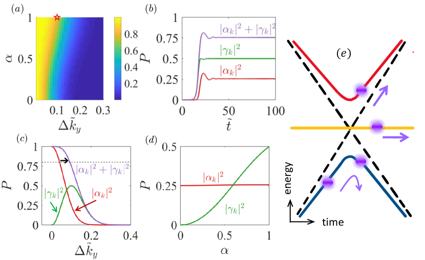
We can now analyze the general - lattice as an interpolation between the idealized two-level and three-level systems, where the coupling between the flat band and the other two bands varies in the range . For convenience, we again initialize electrons in the lower band and examine two transition probabilities: that from the lower to the upper band denoted as and that from the lower to the flat band denoted as . To unveil the effect of increasing the value of from zero, we calculate the two probabilities for and the range of momentum deviation from the Dirac point in the hexagonal Brillouin zone. Figure 2(a) shows the color-coded sum of the two probabilities in the parameter plane , where the range of to generate a high LZT probability increases monotonically with and reaches maximum at , suggesting that the flat band enhances LZT. The time evolution of the two probabilities and their sum is shown in Fig. 2(b). Note that, for , the LZT probabilities and can be determined from Eqs. (63) and (64), respectively. Figure 2(c) shows, for , these two probabilities, together with their sum, versus , where the horizontal dashed line specifies and the arrow indicates the enhancement of the LZT by the flat band. As increases, the value of the characteristic parameter increases, leading to a decrease in the LZT probability to the upper band. However, even when the LZT probability from the lower to the upper bands is effectively zero, there can still be an appreciable transition probability from the lower to the flat band. For example, for , we have . In this case, we have but . Figure 2(d) shows, for fixed , the two probabilities versus . Note that the probability increases monotonically with .
III.2 Morphology and irregular Bloch-Zener oscillations
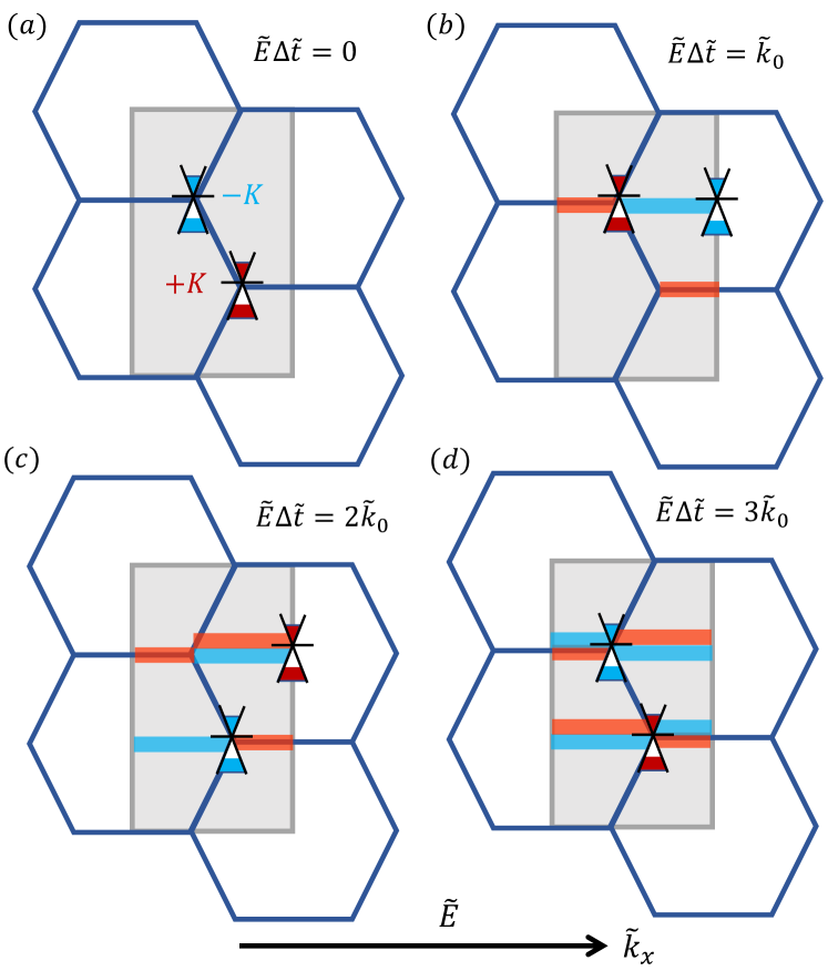
Under a static electric field, the intraband current density will exhibit periodic-like Bloch-Zener oscillations, where the interband contribution can be neglected in the long time situation [44]. Figure 3 provides a schematic picture to explain the origin of the oscillations. Driven by a constant electric field in the positive direction, after , the two Dirac points in the hexagonal Brillouin zone start to move in the same direction, where the gray rectangular region denotes a periodic area in the momentum space, as shown in Fig. 3(a). The edge length of the hexagonal Brillouin zone is in units of , the inverse of the lattice constant. After the time , the valley reaches the original location of the valley, as shown in Fig. 3(b). The reaches the original location of the after the time , as shown in Fig. 3(c). The occurrences of the LZTs associated with the valleys are indicated by the orange and blue horizontal strips, respectively, where the width of excitation zone depends on both the gap size and the magnitude of electric field. At the time , both Dirac points return to their original starting locations, completing one cycle of oscillation during which LZT occurs twice.
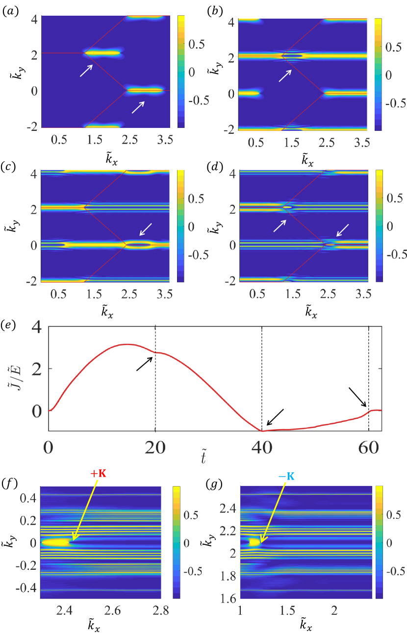
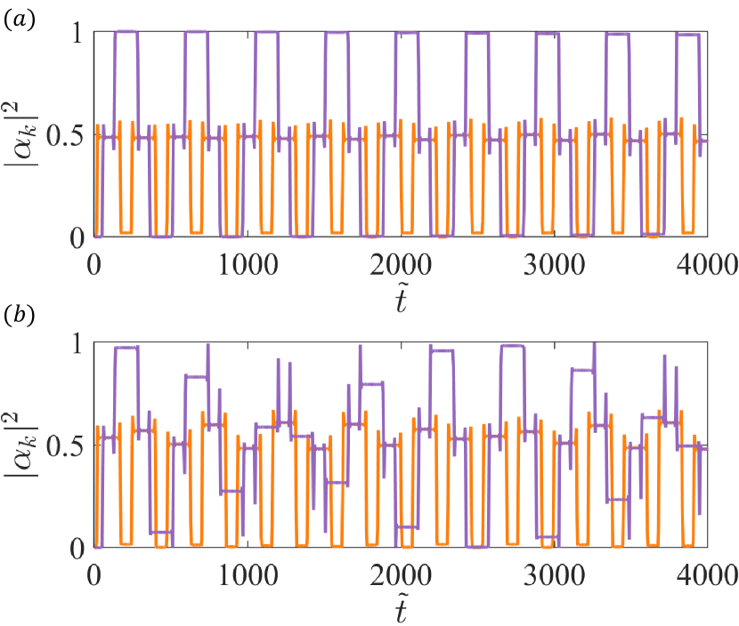
In the vicinity of a Dirac point ( or ) in the momentum space, an infinite set of energy gaps exists where, for different momentum deviations from the Dirac point, the sizes of the energy gap can be quite distinct from the exact energy gap in Eq. (58). As the static electric field in the direction is turned on, the momentum in the direction increases linearly with time, sweeping through all possible values of the component of the momentum in the Brillouin zone, effectively eliminating all the original differences in for different points in the momentum space. However, the various deviations in the component of the momentum, i.e., the different values, still matter and in fact persist because they correspond to different energy gaps. As a result, different values of will lead to different probabilities of LZT, creating a distinct morphology with respect to the LZT probability in the direction of the momentum space at any given time. As an example, Figs. 4(f) and 4(g) present such a morphology after 20 periods of Bloch-Zener oscillations with the magnification about the Dirac points, respectively, where the color-coded values of the differential LZT probability are shown in the plane. An observation is that the LZT morphology, as exemplified in Figs. 4(f) and 4(g), can undergo changes due to the complicated interference pattern between quantum states in different energy bands in the long time, due to the non-deterministic nature of the LZTs with respect to the size of the energy gap. Figure 4(a) presents such a morphology after time (immediately after the electric field is turned on) within one period of the Bloch-Zener oscillation. Three examples are illustrated in Fig. 4(b-d), where the color-coded values of at three time instants: , and , are displayed. The morphological changes in the LZTs are concentrated in the vertical neighborhoods of the Dirac points, whereas the values of in most of the momentum space remain unchanged.
A remarkable phenomenon is that, when a change in the LZT morphology occurs, some experimentally measurable quantities such as the current density can undergo a sudden change as well. To be concrete, we focus on the current density associated with Bloch-Zener oscillations, which is dominantly determined by the intraband behaviors [44]. Suppose that, initially, the electrons are prepared in the lower band. Due to the change in the LZT morphology and the mutual switching between the Dirac points , the dependence of the probabilities for the electrons to be in the upper band on the momentum will change, and this will lead to a sudden change in the current density that is contributed to by all the momenta in the Brillouin zone. Note from Figs. 4(b-d) that the changes in the LZT morphology are pronounced only near the original Dirac points where an LZT is most likely to occur, while there are no such changes for most of the momentum space. Since the current density is the integration over the entire Brillouin zone, the resulting change in the current density will be quite “subtle” in the sense that it will not be a discontinuous change in the current density itself but a non-smooth change (or, equivalently, a discontinuous change in the time derivative of the current density). Such nonsmooth changes have indeed been numerically observed, as shown in Fig. 4(a), where the arrows and the vertical dashed lines indicate the three time instants at which such a change occurs, corresponding to the distinct LZT morphology in Figs. 4(b-d), respectively. To compare irregular and periodic Bloch-Zener oscillations, we also study the oscillations resulting from near ideal LZTs in the momentum space (Appendix A).
IV Landau-Zener-Stückelberg interferometry in - lattice
IV.1 Two- and three-level models
The dynamical evolution of the wavefunction in the - lattice for () driven by a static electric field can be described by the Hamiltonian of a strongly periodically driven two- or three-level system, as demonstrated in Appendix C. According to the adiabatic-impulse theory [12, 11], the quantum evolution can be decomposed into adiabatic evolution and non-adiabatic LZTs, where the former occurs most of the time but the latter occur on a short time scale. For , under the adiabatic impulse approximation, this physical picture still applies. Specifically, for the adiabatic evolution, the eigenenergy spectrum is independent of the value of the lattice coupling parameter , so the adiabatic phase for is similar to that for . Insights into the LZTs can be gained by numerically calculating the time evolution of the transition probability and in - lattice, as exemplified in Fig. 2.
The adiabatic evolution of the wavefunction generates an adiabatic phase, while the LZTs lead to a non-adiabatic phase. To gain insights, consider the double passage case in a strongly periodically driven two-level system, where two successive transitions are required for a particle initiated from an eigenstate in the lower band to reach the upper band with probability one, as exemplified in Fig. 5(a). In this case, after two successive LZTs, the transition probability to the upper band is given by [48, 11] (Appendix B.1)
| (66) | ||||
| (67) |
where is the first-time LZT probability given by Eq. (59) and is the Stückelberg that consists of two components: the adiabatic phase between two consecutive LZTs and the non-adiabatic phase, i.e., the Stokes phase at the transition. There are two distinct cases. The first is
| (68) |
corresponding to constructive interference [11] because, after one driving period, the maximum transition probability to the upper band is , which is twice the average transition probability over one period. The second case is
| (69) |
giving rise to destructive interference [11] as after one driving period.
Our equivalence analysis in Appendix C and the treatment of the strongly periodically driven two-level system in Appendix B.1 give that, for in the - lattice, the adiabatic phase is given by
| (70) |
where is defined in Eq. (17) and depends on the electric field and the momentum deviation from . The non-adiabatic phase is determined by the linearized LZT Hamiltonian about the Dirac points :
| (71) |
where is determined by the LZT characteristic parameter as , as given by Eq. (60). It can be seen that the Stückelberg phase also depends on the electric field and the momentum deviation from .
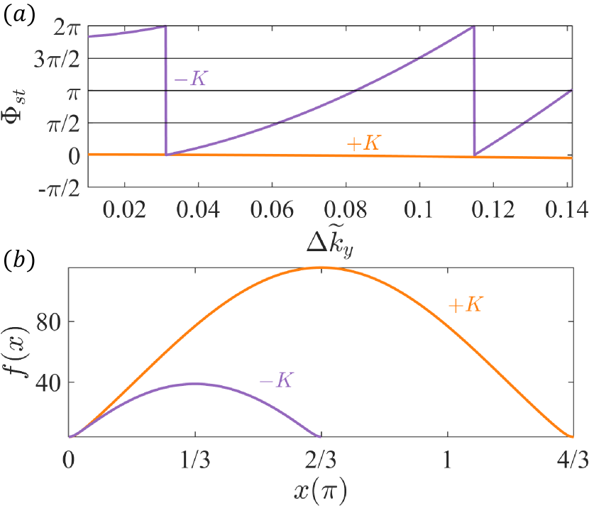
Figure 6(a) shows the Stückelberg phase for two types of initial momentum values for . For LZTs starting near the Dirac point , the Stückelberg phase is non-adiabatic and approximately independent of the momentum deviation , while for , the phase is adiabatic so it depends on the momentum deviation [Eq. (71)]. More specifically, for LZTs starting from the Dirac points , the adiabatic phase between two successive LZTs is
| (72) | ||||
| (73) |
where the functions and are given by
| (74) |
with , , measured from , and . Figure 6(b) shows the adiabatic phase measured from the Dirac points . Since the integration of has a relatively large value, the adiabatic phase is nearly constant for different momentum deviation for , whereas is sensitive to . The adiabatic phase also depends on the electric field . (More elaborate details can be found in Appendix D.)
For , a flat band arises in addition to the two Dirac cone bands. Figure 7 shows the representative time evolution of the transition probabilities and for . Exploiting the equivalence of the dice lattice driven by a constant electric field to a strongly periodically driven three-level system (Appendix C), we have that, after one Bloch-Zener oscillation period (two successive LZTs), the occupation probability of the upper, flat and lower bands are given by (Appendix B.2)
| (75) | |||
| (76) | |||
| (77) |
with the normalization constraint , where
| (78) |
For the upper band, corresponds to constructive interference and leads to destructive interference [Eq. (75)]. For the flat band, gives [Eq. (76)]. For , we have with . Note that the Stokes phase disappears in this case based on the non-adiabatic transition matrix [13]. From Eq. (71), for , the Stokes phase is a small constant: . As a result, we have .
IV.2 Morphology selection
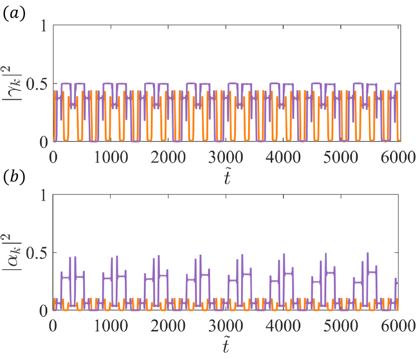
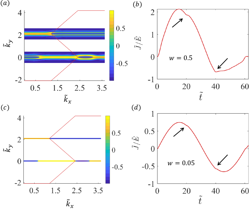
So far, we have numerically observed the complex LZT morphology and found a relationship between morphological changes and irregular Bloch-Zener oscillations. In addition, we have analyzed the interference phases in - lattice based on the equivalence between the lattice subject to a constant electric field and strongly periodically driven two- or three level systems. We have found that the Stückelberg phase (adiabatic phase) of LZTs starting from the Dirac point is nearly independent of the momentum deviation , i.e., the energy gap, while the phase starting from is sensitive to . For , destructive interference among the quantum states from different bands arises for . For , only corresponds to destructive interference. These findings suggest a principle of morphology selection for : setting or for LZT starting from the valley will result in two distinct types of LZT morphology, as illustrated in Figs. 8 and 9, respectively. As analyzed in Appendix A, ideal LZTs in the Brillouin zone lead to periodic and regular Bloch-Zener oscillations. The destructive interference has a similar effect to that of ideal LZTs. AS a result, the resulting morphology pattern can improve the regularity of Bloch-Zener oscillations.
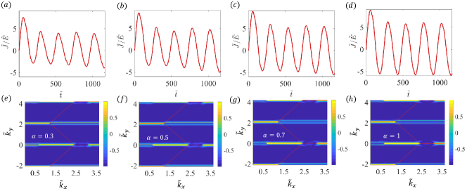
Figure 8 shows, for and four different types of - lattices, the irregular Bloch-Zener oscillations and the corresponding representative LZT morphology at a given time in the momentum space. It can be seen that the Bloch-Zener oscillations shown in Figs. 8(a-d) are somewhat irregular - they are mostly regular. The destructive interference pattern of LZTs starting from the valley in the momentum space is shown in Figs. 8(e-h) with . For another type of morphology with , the Bloch-Zener oscillations are more irregular. For example, for , the oscillations can be strongly irregular or “chaotic,” as exemplified in Figs. 9(b) and 9(c). In this case, for , the interference pattern associated with the LZTs starting from the valley changes from destructive to non-destructive, as shown in Figs. 9(d-f). In both cases, the morphology of LZTs starting from the valley changes little due to the sensitivity to the momentum deviation.
V Discussion
Bloch or Bloch-Zener oscillations, in addition to being a fundamental phenomenon in solid state physics, practically provides the foundation to convert a direct current into an oscillating current in the terahertz frequency regime [24]. Research in the past decade or so has suggested that, in 2D multiband materials, Bloch-Zener oscillations can be vulnerable to Landau-Zener transition or tunneling [29, 30, 34, 33, 35, 36]. Is this generally true? The question is important to physics and our present work has provided two-fold answers: yes LZTs can indeed affect the Bloch oscillations but what is destroyed is not the oscillations themselves but just the perfect time periodicity of the oscillations; no because the irregular oscillations can persist even with frequent occurrences of LZTs. In fact, approximately periodic Bloch-Zener oscillations can be maintained if the LZTs are near ideal such that they result in a near-one probability for the electrons to switch into a different band or when near destructive interference arises between the quantum states in different energy bands. Nonsmooth or irregular behaviors in the current density arise when the LZTs are not ideal and the interference is partially destructive.
Our study encompasses the entire spectrum of a class of 2D Dirac materials modeled by - lattices. We have found that the set of points in the 2D momentum space near a Dirac point at which LZTs occur can possess a complex morphology, and it is the change in the morphology that results in irregular Bloch-Zener oscillations. Theoretically, when driven by a static electric field, an - lattice is equivalent the Landau-Zener-Stückelberg interferometry. Specifically, the lattice (graphene) is effectively a two-level periodically driven quantum system while the general - lattice for is equivalent to a three-level periodically driven system. For the three-level system, we have exploited the concept of Stückelberg phase from the adiabatic impulse theory to understand the LZTs that occur in the neighborhoods of the Dirac points in distinct valleys.
In the - lattice, a non-zero coupling parameter induces a flat band in between the positive and negative energy bands, effectively resulting a three-level system. After the first LZT in Fig. 2, the quantum state is a superposition of the three energy bands and the LZT is enhanced by the flat band (compared with the two-level case). For subsequent LZTs (e.g., as shown in Figs. 8 and 9), the flat band modifies the Stückelberg phase for destructive interference in the three-band interferometry (compared with the two-band one). More specifically, for , the destructive interference corresponds to from Eq. (66). For , the destructive interference means only and the case is excluded from Eqs. (75-77). For , the behavior of destructive interference is obtained numerically, as shown in Figs. 8 and 9, which is slightly different from the case, especially in Figs. 9(e,f). Taken together, a nonzero modifies the physical picture from two- to three-band quantum interference: it generates a flat band in the original two-level system, creates three-band interferometry, enhances LZT in the momentum space around the Dirac points, and modifies destructive interference.
Theoretically, the asymmetrical morphology pattern around the points results from the different characteristics of the Stückelberg phases . As shown in Fig. 6(a), is nearly constant with measured from the Dirac point after two LZTs and changes greatly with from . Different values of the interference phase give distinct interference patterns, such as constructive, destructive, and mixed quantum interference (neither constructive nor destructive) in the momentum space, as exemplified in Fig. 4(c).
For LZTs with a near unity transition probability, which can occur for an infinitesimal energy gap, the points make the same contribution to the Bloch oscillations. However, slightly away from the Dirac points where the energy gap is no longer infinitesimal, the contributions differ. The reason why the Bloch oscillations around are more prominent compared with those around the point lies in the interference phase . In particular, the LZTs from the point with different momentum deviation are in phase with each other, as shown in Fig. 6(a). However, the LZTs measured from the point are out of phase, so the contributions to the Bloch oscillations cancel each other to some degree.
The irregular Bloch-Zener oscillations in the average current density integrated over the Brillouin zone arise from the LZTs induced by different energy gaps associated with the momentum deviation measured from Dirac points. In the - lattice, there is an alternative way to induce an energy gap between the valence and conduction bands by adding the positive (negative) onsite energy on the A (B) sublattice [49, 50]. Because of the sensitive dependence of the LZT on the size of the momentum-dependent energy gap, irregularities in the LZTs are anticipated, so are the irregular Bloch-Zener oscillations.
Experimentally, it may be feasible to observe at least the first peak of the Bloch-Zener oscillation in ballistic time [37]. To probe into the momentum-space morphology associated with LZTs and to directly observe the irregular Bloch-Zener oscillations in a longer time interval in Dirac material systems remain to be difficult at the present. Alternatively, it may be possible to use quantum simulators [51, 52] by exploring equivalent optical systems [20]. In the past, Bloch oscillations have been experimentally studied in photonic systems [21, 53, 23, 35, 54]. The observation of Bloch-Zener oscillations and Landau-Zener tunneling in photonic graphene [35] is particularly relevant to possible experimental checks of our findings. In this artificial Dirac system, the wave packet of light is driven by an index gradient on a non-adiabatic basis and the two sublattices are subjected to a potential imbalance. When the momentum deviation is zero from a Dirac point and the index gradient is applied in a specific direction, perfect (ideal) LZT with transition probability one can occur due to the zero energy gap. However, when the index gradient is applied in the orthogonal direction, the LZT becomes imperfect (non-ideal) due to the non-zero gap. Our work suggests that, if the time evolution of the wavefunction in photonic graphene can be approximated as constituting two processes: adiabatic evolution and non-adiabatic LZT, in principle the Stückelberg phase can be calculated to choose the appropriate index gradient value to create destructive interference between the quantum states in the upper and lower energy bands. It may thus be possible to generate destructive interference to obtain a near-ideal LZT. Our work predicts that, in this case, the resulting Bloch-Zener oscillations will become more periodic. Photonic graphene may be a feasible experimental testbed for these phenomena.
Acknowledgment
We thank Drs. Chen-Di Han and Cheng-Zhen Wang as well as Prof. Liang Huang for valuable discussions. This work was supported by AFOSR under Grant No. FA9550-21-1-0186.
Appendix A LZT morphology and irregular Bloch-Zener oscillations
To further appreciate the interplay between LZT morphology and irregular Bloch-Zener oscillations, we consider two kinds of momentum integration regions about the Dirac points, as shown in Figs. 10(a) and 10(c), respectively. The resulting time evolution of the current density is shown in Figs. 10(b) and 10(d), respectively. For the case in Fig. 10(c), the LZTs are near ideal, generating less irregular Bloch-Zener oscillations in Fig. 10(d).
Appendix B Adiabatic impulse theory
B.1 Two-level systems
The Hamiltonian under a periodic driving in the non-adiabatic basis has the form [11]
| (79) |
where the driving produces a periodic time evolution of the eigenenergy spectrum:
| (80) |
If the bias of the driving is nonzero: , one period of the evolution of the energy contains two peaks [11] that are in the time intervals and , respectively. The quantum dynamical process can be understood by using the adiabatic impulse theory [12, 11]. According to this theory, the dynamical process can be approximated as the adiabatic evolution from to and from to , which are described by unitary transformation matrices and , respectively, and non-adiabatic transitions at and that are described by the same non-adiabatic transition matrix . After one period, the quantum state under the adiabatic basis can be written as [11]
| (81) |
When the driving signal is linearized about the transition point as , the non-adiabatic transition matrix in the adiabatic basis is [11]
| (84) |
where is the first LZT probability of the upper band defined by Eq. (59), , and is the Stokes phase. The adiabatic evolution matrix in the adiabatic basis is
| (89) |
where and are the adiabatic phases given by
| (90) |
In the adiabatic basis, the total transform matrix after one period is [11]
| (93) |
where the matrix elements are
| (94) | |||
and is the Stückelberg phase. If the initial state is
| (95) |
the quantum state after one period will be
| (96) |
with the transition probabilities
| (97) | |||
| (98) |
which satisfy the normalization constraint . From Eq. (97), it can be seen that whether the transition is complete depends only on the Stokes phase and the adiabatic phase between two consecutive LZTs. Specifically, corresponds to destructive interference between the quantum states in the upper and lower bands while corresponds to constructive interference.
B.2 Three-level systems
A periodically driven three-level system is described by
| (99) |
where the time evolution of the positive and negative energy is given by Eq. (80) except for the extra flat band . A previous work [13] provided the non-adiabatic transition matrix in the adiabatic basis when the driving signal is linearized about the transition point as :
| (103) |
where all , and are constants:
| (104) |
and
| (105) |
The adiabatic evolution matrix of the three-level system is
| (112) |
The total transform matrix is
| (116) |
where
| (117) |
with
| (118) |
for . Suppose the initial quantum state is
| (119) |
After one period, the quantum state becomes
| (120) |
The occupied probabilities of the upper, flat and lower bands after one period are given by
| (121) | |||
| (122) | |||
| (123) |
respectively, where , and with the constraint . According to Eq. (121), for the upper band, we have that corresponds to constructive interference and to destructive interference. For the flat band, corresponds to destructive interference, as stipulated by Eq. (122). For , the flat band leads to an LZT with probability away from zero except for The Stokes phase defined by Eq. (71) depends only on the parameter (). Numerically, we obtain . In spite of the small phase deviation due to the Stokes phase , corresponds approximately to destructive interference regardless of the existence of a flat band. However, does not represent destructive interference in the three-level system.
Appendix C Equivalence of - lattice to strongly periodically driven two- or three-level systems
When a static electric field is applied to an - lattice, the time evolution of the wavefunction can be obtained by using the adiabatic impulse theory [12, 11]. For graphene () and the dice lattice (), the tight-binding Hamiltonians are, respectively,
| (124) |
and
| (125) |
where and are the Pauli matrices for pseudospin-1/2 quasiparticles in graphene, and are the corresponding matrices from pseudospin-1 quasiparticles in the dice lattice, and
| (126) |
The eigenenergy spectrum of graphene is . For the dice lattice, there is a flat band . The time evolution of nonzero energy band of both graphene and dice lattice has the common form for the upper and lower bands:
| (127) |
where
| (128) |
Equation (127) has the same mathematical form as that for a strongly periodically driven two-level system [Eq. (80)].
A theoretical approach to dealing with a strongly periodically driven two-level system is the adiabatic and impulse approximation [12, 11], which is valid in the regime of strong field
| (129) |
Equations (127) and (80) give and , rendering applicable the adiabatic and impulse approximation. The idea of the analysis is to decompose the time evolution of system into an adiabatic evolution when it is far from the points of avoided-crossing and non-adiabatic process in the vicinity of these points.
For adiabatic evolution in graphene, the adiabatic phase in the wavefunction depends on the integral . The dice lattice has the same energy and the flat band corresponds to a zero adiabatic phase . Thus, for the upper and lower bands in both graphene and dice lattice, the adiabatic phase has the same mathematical form as that for the periodically driven two- and three-level system, respectively.
For the non-adiabatic transition process in graphene or dice lattice, the effective Hamiltonian about the Dirac points is the standard or the three-level Landau-Zener Hamiltonian. Concretely, we can show that the Hamiltonian for graphene and dice lattice, given by Eqs. (124) and (125), can be written as the standard Landau-Zener Hamiltonian for two- and three-level systems, respectively, as
| (130) | ||||
| (131) |
through some unitary transformation. In particular, the requirement is to have for graphene and for dice lattice. These transformations can be realized by rotating the original Hamiltonian in two steps since the physical observable does not change after a unitary transformation. First, we rotate the Hamiltonian along the anticlockwise direction with around the axis to get , where for graphene and for dice lattice. Second, we rotate the Hamiltonian along the anticlockwise direction with around the -axis to obtain , where for graphene and for dice lattice. The total unitary transformations for graphene and dice lattice are
| (132) | ||||
| (133) |
respectively.
As for Hamiltonian expansion about Dirac points, firstly, we expand Hamiltonian in the direction about the Dirac points with
| (134) |
leading to
| (135) |
With the unitary transformation in Eq. (132) we obtain the approximate Hamiltonian as given by
| (136) |
with
| (137) |
For the dice lattice, with the total unitary transformation in Eq. (133) we have the approximate Hamiltonian as
| (138) |
From Eqs. (136) and (138), we translate the momentum to the Dirac points as
| (139) |
Setting with starting from origin, we obtain, about ,
| (142) | ||||
| (143) |
where the second-order term has been neglected. For graphene, the effective Hamiltonian about the Dirac points is
| (144) |
which is the standard Landau-Zener Hamiltonian [45]. For the dice lattice, the effective Hamiltonian is
| (145) |
which is the Hamiltonian of the three-level Landau-Zener model [13]. In the vicinity of the Dirac points, the non-adiabatic Landau-Zener transition in graphene (dice lattice) induced by a constant electric field thus shares the same quantum dynamical law as that in the adiabatic impulse theory [12, 11].
For the general - for , the picture of the quantum dynamical evolution as consisting of adiabatic evolution and non-adiabatic LZTs is still applicable, because the eigenenergy spectrum is independent of the lattice coupling parameter . In fact, adiabatic phase with is the same as that for . For the non-adiabatic process, the first LZT has been numerically calculated, as shown in Fig. 2. Consequently, under the adiabatic impulse approximation, the dynamical evolution of the - lattice is identical to that of the wavefunction of a strongly periodically driven three-level system.
Appendix D Stückelberg phase with electric field
| weaker | ||||||
| 100 | 0.0725 | 141 | 0.0514 | 193 | 0.0376 | 0.0072 |
| 121 | 0.06 | 157 | 0.0462 | 198 | 0.0366 | 0.0065 |
| 126 | 0.0576 | 162 | 0.0448 | 219 | 0.0332 | 0.006 |
| 131 | 0.0554 | 167 | 0.0434 | 229 | 0.0317 | 0.0059 |
| 136 | 0.0533 | 188 | 0.0386 | 260 | 0.0279 | 0.0053 |
| weaker | ||||
| 118 | 0.0614 | 175 | 0.0415 | 0.0069 |
| 144 | 0.0504 | 180 | 0.0403 | 0.0068 |
| 149 | 0.0487 | 185 | 0.0392 | 0.0067 |
| 154 | 0.0471 | 206 | 0.0352 | 0.0062 |
| 211 | 0.0344 | 247 | 0.0294 | 0.0042 |
| 216 | 0.0336 | 257 | 0.0282 | 0.0035 |
| 242 | 0.03 | 278 | 0.0261 | 0.003 |
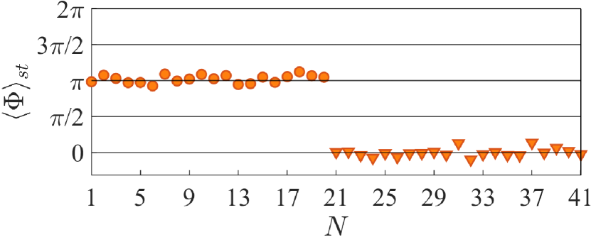
Because the Stückelberg phase is near constant for LZTs starting from the valley, as exemplified in Fig. 6(a), we define the average Stückelberg phase over the range of the momentum deviation as determined by . Although the Stückelberg or adiabatic phase is sensitive to the magnitude of the electric field [Eqs. (72) and (IV.1)], we numerically test two sets of electric fields to produce the average Stückelberg phase from the valley around or zero, as shown in Fig. 11 for the electric field values listed in Tabs. 1 and 2 for :
| (146) |
In Tabs. 1 and 2, the field values are determined based on the destructive interference pattern of LZTs starting from the valley for such as the orange traces in Figs. 5(a) and 5(b) and are tested in the range of momentum deviation determined by . For , two types of behaviors can arise. In the first type, for , for the electric field values from Tab. 1, the LZT probability can no longer reach zero after two successive LZTs, i.e., no destructive interference. In this case, the Stückelberg phase is , as shown by the filled circles in Fig. 6(b). The second type occurs for field values from Tab. 2, where still displays a near-destructive interference pattern for any . In this case, the Stückelberg phase is , as shown by the filled triangles in Fig. 6(b).
References
- Landau [1932] L. Landau, On the theory of transfer of energy at collisions II, Phys. Z. Sowjetunion 2, 118 (1932).
- Zener [1932] C. Zener, Non-adiabatic crossing of energy levels, Proc. R. Soc. London Ser. A 137, 696 (1932).
- Kok et al. [2007] P. Kok, W. J. Munro, K. Nemoto, T. C. Ralph, J. P. Dowling, and G. J. Milburn, Linear optical quantum computing with photonic qubits, Rev. Mod. Phys. 79, 135 (2007).
- Graham et al. [2022] T. Graham, Y. Song, J. Scott, C. Poole, L. Phuttitarn, K. Jooya, P. Eichler, X. Jiang, A. Marra, B. Grinkemeyer, et al., Multi-qubit entanglement and algorithms on a neutral-atom quantum computer, Nature 604, 457 (2022).
- Berke et al. [2022] C. Berke, E. Varvelis, S. Trebst, A. Altland, and D. P. DiVincenzo, Transmon platform for quantum computing challenged by chaotic fluctuations, Nat. Commun. 13, 1 (2022).
- Niu et al. [1996] Q. Niu, X.-G. Zhao, G. A. Georgakis, and M. G. Raizen, Atomic Landau-Zener tunneling and Wannier-Stark ladders in optical potentials, Phys. Rev. Lett. 76, 4504 (1996).
- Salger et al. [2007] T. Salger, C. Geckeler, S. Kling, and M. Weitz, Atomic Landau-Zener tunneling in Fourier-synthesized optical lattices, Phys. Rev. Lett. 99, 190405 (2007).
- Liu et al. [2021] W.-X. Liu, T. Wang, X.-F. Zhang, and W.-D. Li, Time-domain Landau-Zener-Stückelberg-Majorana interference in an optical lattice clock, Phys. Rev. A 104, 053318 (2021).
- Kervinen et al. [2019] M. Kervinen, J. E. Ramírez-Muñoz, A. Välimaa, and M. A. Sillanpää, Landau-Zener-Stückelberg interference in a multimode electromechanical system in the quantum regime, Phys. Rev. Lett. 123, 240401 (2019).
- Ivakhnenko et al. [2018] O. V. Ivakhnenko, S. N. Shevchenko, and F. Nori, Simulating quantum dynamical phenomena using classical oscillators: Landau-Zener-Stückelberg-Majorana interferometry, latching modulation, and motional averaging, Sci. Rep. 8, 1 (2018).
- Shevchenko et al. [2010] S. N. Shevchenko, S. Ashhab, and F. Nori, Landau–zener–stückelberg interferometry, Phys. Rep. 492, 1 (2010).
- Damski and Zurek [2006] B. Damski and W. H. Zurek, Adiabatic-impulse approximation for avoided level crossings: From phase-transition dynamics to Landau-Zener evolutions and back again, Phys. Rev. A 73, 063405 (2006).
- Carroll and Hioe [1986] C. Carroll and F. Hioe, Generalisation of the Landau-Zener calculation to three levels, J. Phys. A Math. Gen. 19, 1151 (1986).
- Khomeriki and Flach [2016] R. Khomeriki and S. Flach, Landau-Zener Bloch oscillations with perturbed flat bands, Phys. Rev. Lett. 116, 245301 (2016).
- Parkavi et al. [2021] J. R. Parkavi, V. Chandrasekar, and M. Lakshmanan, Stable Bloch oscillations and Landau-Zener tunneling in a non-hermitian PT-symmetric flat-band lattice, Phys. Rev. A 103, 023721 (2021).
- Bloch [1928] F. Bloch, Quantum mechanics of electrons in crystal lattices, Z. Phys 52, 555 (1928).
- Zener [1934] C. Zener, A theory of the electrical breakdown of solid dielectrics, Proc. R. Soc. London Ser. A 145, 523 (1934).
- Waschke et al. [1993] C. Waschke, H. G. Roskos, R. Schwedler, K. Leo, H. Kurz, and K. Köhler, Coherent submillimeter-wave emission from Bloch oscillations in a semiconductor superlattice, Phys. Rev. Lett. 70, 3319 (1993).
- Morandotti et al. [1999] R. Morandotti, U. Peschel, J. Aitchison, H. Eisenberg, and Y. Silberberg, Experimental observation of linear and nonlinear optical Bloch oscillations, Phys. Rev. Lett. 83, 4756 (1999).
- Sapienza et al. [2003] R. Sapienza, P. Costantino, D. Wiersma, M. Ghulinyan, C. J. Oton, and L. Pavesi, Optical analogue of electronic Bloch oscillations, Phys. Rev. Lett. 91, 263902 (2003).
- Trompeter et al. [2006] H. Trompeter, W. Krolikowski, D. N. Neshev, A. S. Desyatnikov, A. A. Sukhorukov, Y. S. Kivshar, T. Pertsch, U. Peschel, and F. Lederer, Bloch oscillations and Zener tunneling in two-dimensional photonic lattices, Phys. Rev. Lett. 96, 053903 (2006).
- Ghulinyan et al. [2005] M. Ghulinyan, C. J. Oton, Z. Gaburro, L. Pavesi, C. Toninelli, and D. S. Wiersma, Zener tunneling of light waves in an optical superlattice, Phys. Rev. Lett. 94, 127401 (2005).
- Block et al. [2014] A. Block, C. Etrich, T. Limboeck, F. Bleckmann, E. Soergel, C. Rockstuhl, and S. Linden, Bloch oscillations in plasmonic waveguide arrays, Nat. Commun. 5, 1 (2014).
- Schubert et al. [2014] O. Schubert, M. Hohenleutner, F. Langer, B. Urbanek, C. Lange, U. Huttner, D. Golde, T. Meier, M. Kira, S. W. Koch, et al., Sub-cycle control of terahertz high-harmonic generation by dynamical Bloch oscillations, Nat. Photonics 8, 119 (2014).
- Fahimniya et al. [2021] A. Fahimniya, Z. Dong, E. I. Kiselev, and L. Levitov, Synchronizing Bloch-oscillating free carriers in Moiré flat bands, Phys. Rev. Lett. 126, 256803 (2021).
- Dreisow et al. [2009] F. Dreisow, A. Szameit, M. Heinrich, T. Pertsch, S. Nolte, A. Tünnermann, and S. Longhi, Bloch-Zener oscillations in binary superlattices, Phys. Rev. Lett. 102, 076802 (2009).
- Lim et al. [2012] L.-K. Lim, J.-N. Fuchs, and G. Montambaux, Bloch-Zener oscillations across a merging transition of dirac points, Phys. Rev. Lett. 108, 175303 (2012).
- Zhang et al. [2021] Y. Zhang, Z. Li, L. Qin, C. Yang, H. Lu, J. Zhang, X. Zhao, Z. Zhu, et al., Band evolution and Landau-Zener Bloch oscillations in strained photonic rhombic lattices, Opt. Exp. 29, 37503 (2021).
- Breid et al. [2006] B. Breid, D. Witthaut, and H. Korsch, Bloch–Zener oscillations, New J. Phys. 8, 110 (2006).
- Breid et al. [2007] B. Breid, D. Witthaut, and H. Korsch, Manipulation of matter waves using Bloch and Bloch–Zener oscillations, New J. Phys. 9, 62 (2007).
- Morsch et al. [2001] O. Morsch, J. Müller, M. Cristiani, D. Ciampini, and E. Arimondo, Bloch oscillations and mean-field effects of Bose-Einstein condensates in 1d optical lattices, Phys. Rev. Lett. 87, 140402 (2001).
- Venkatesh et al. [2009] B. P. Venkatesh, M. Trupke, E. Hinds, and D. O’Dell, Atomic Bloch-Zener oscillations for sensitive force measurements in a cavity, Phys. Rev. A 80, 063834 (2009).
- Lim et al. [2015] L.-K. Lim, J.-N. Fuchs, and G. Montambaux, Geometry of Bloch states probed by Stückelberg interferometry, Phys. Rev. A 92, 063627 (2015).
- Kling et al. [2010] S. Kling, T. Salger, C. Grossert, and M. Weitz, Atomic Bloch-Zener oscillations and Stückelberg interferometry in optical lattices, Phys. Rev. Lett. 105, 215301 (2010).
- Sun et al. [2018] Y. Sun, D. Leykam, S. Nenni, D. Song, H. Chen, Y. D. Chong, and Z. Chen, Observation of valley Landau-Zener-Bloch oscillations and pseudospin imbalance in photonic graphene, Phys. Rev. Lett. 121, 033904 (2018).
- Chang et al. [2022] Y.-J. Chang, Y.-H. Lu, Y.-Y. Yang, Y. Wang, W.-H. Zhou, X.-W. Wang, and X.-M. Jin, Inhibition and reconstruction of Zener tunneling in photonic honeycomb lattices, Adv. Mater. , 2110044 (2022).
- Rosenstein et al. [2010] B. Rosenstein, M. Lewkowicz, H.-C. Kao, and Y. Korniyenko, Ballistic transport in graphene beyond linear response, Phys. Rev. B 81, 041416 (2010).
- Kolovsky and Bulgakov [2013] A. R. Kolovsky and E. N. Bulgakov, Wannier-Stark states and Bloch oscillations in the honeycomb lattice, Phys. Rev. A 87, 033602 (2013).
- Raoux et al. [2014a] A. Raoux, M. Morigi, J.-N. Fuchs, F. Piéchon, and G. Montambaux, From dia-to paramagnetic orbital susceptibility of massless fermions, Phys. Rev. Lett. 112, 026402 (2014a).
- Illes et al. [2015] E. Illes, J. Carbotte, and E. Nicol, Hall quantization and optical conductivity evolution with variable Berry phase in the - model, Phys. Rev. B 92, 245410 (2015).
- Bercioux et al. [2009] D. Bercioux, D. Urban, H. Grabert, and W. Häusler, Massless Dirac-Weyl fermions in a optical lattice, Phys. Rev. A 80, 063603 (2009).
- Raoux et al. [2014b] A. Raoux, M. Morigi, J.-N. Fuchs, F. Piéchon, and G. Montambaux, From dia-to paramagnetic orbital susceptibility of massless fermions, Phys. Rev. Lett. 112, 026402 (2014b).
- Kittel and McEuen [2018] C. Kittel and P. McEuen, Kittel’s Introduction to Solid State Physics (John Wiley & Sons, 2018).
- Dóra and Moessner [2010] B. Dóra and R. Moessner, Nonlinear electric transport in graphene: quantum quench dynamics and the schwinger mechanism, Phys. Rev. B 81, 165431 (2010).
- Wang et al. [2017] C.-Z. Wang, H.-Y. Xu, L. Huang, and Y.-C. Lai, Nonequilibrium transport in the pseudospin-1 dirac-weyl system, Phys. Rev. B 96, 115440 (2017).
- Tayebirad et al. [2010] G. Tayebirad, A. Zenesini, D. Ciampini, R. Mannella, O. Morsch, E. Arimondo, N. Lörch, and S. Wimberger, Time-resolved measurement of landau-zener tunneling in different bases, Phys. Rev. A 82, 013633 (2010).
- Vitanov and Garraway [1996] N. Vitanov and B. Garraway, Landau-Zener model: Effects of finite coupling duration, Phys. Rev. A 53, 4288 (1996).
- Liang et al. [2020] S. Liang, Z.-C. Li, W. Zhang, L. Zhou, and Z. Lan, Stückelberg interferometry using spin-orbit-coupled cold atoms in an optical lattice, Phys. Rev. A 102, 033332 (2020).
- Abranyos et al. [2021] Y. Abranyos, G. Gumbs, and O. Berman, Superfluidity of dipolar excitons in a double layer of alpha-t3 with a mass term, in APS March Meeting Abstracts, Vol. 2021 (2021) pp. U71–063.
- Berman et al. [2022] O. L. Berman, G. Gumbs, G. P. Martins, and P. Fekete, Superfluidity of dipolar excitons in a double layer of - t 3 with a mass term, Nanomaterials 12, 1437 (2022).
- Trabesinger [2012] A. Trabesinger, Quantum simulation, Nat. Phys. 8, 263 (2012).
- Georgescu et al. [2014] I. M. Georgescu, S. Ashhab, and F. Nori, Quantum simulation, Rev. Mod. Phys. 86, 153 (2014).
- Corrielli et al. [2013] G. Corrielli, A. Crespi, G. Della Valle, S. Longhi, and R. Osellame, Fractional Bloch oscillations in photonic lattices, Nat. Commun. 4, 1 (2013).
- Xu et al. [2016] Y.-L. Xu, W. S. Fegadolli, L. Gan, M.-H. Lu, X.-P. Liu, Z.-Y. Li, A. Scherer, and Y.-F. Chen, Experimental realization of Bloch oscillations in a parity-time synthetic silicon photonic lattice, Nat. Commun. 7, 1 (2016).