Recursive Speculative Decoding:
Accelerating LLM Inference via Sampling Without Replacement

Abstract

Speculative decoding is an inference-acceleration method for large language models (LLMs) where a small language model generates a draft-token sequence which is further verified by the target LLM in parallel. Recent works have advanced this method by establishing a draft-token tree, achieving superior performance over a single-sequence speculative decoding. However, those works independently generate tokens at each level of the tree, not leveraging the tree’s entire diversifiability. Besides, their empirical superiority has been shown for fixed length of sequences, implicitly granting more computational resource to LLM for the tree-based methods. None of the existing works has conducted empirical studies with fixed target computational budgets despite its importance to resource-bounded devices. We present Recursive Speculative Decoding (RSD), a novel tree-based method that samples draft tokens without replacement and maximizes the diversity of the tree. During RSD’s drafting, the tree is built by either Gumbel-Top-$k$ trick that draws tokens without replacement in parallel or Stochastic Beam Search that samples sequences without replacement while early-truncating unlikely draft sequences and reducing the computational cost of LLM. We empirically evaluate RSD with Llama 2 and OPT models, showing that RSD outperforms the baseline methods, consistently for fixed draft sequence length and in most cases for fixed computational budgets at LLM.

1 Introduction

Large language models (LLMs) (Touvron et al., 2023; Zhang et al., 2022; Brown et al., 2020; Achiam et al., 2023; Jiang et al., 2023) have gained popularity due to their outstanding achievements with high-quality text generation, which has drastically increased demands for faster text generation. However, auto-regressive nature of LLMs limits text generation to produce a single token at a time and often suffers from memory-bandwidth bottleneck, which leads to slower inference (Shazeer, 2019). translation (Xiao et al., 2023).

Speculative decoding (Chen et al., 2023; Leviathan et al., 2023) has emerged as a solution for LLM inference acceleration by leveraging the innate parallelizability of the transformer network (Vaswani et al., 2017). This decoding method utilizes a draft model, i.e., a smaller language model, to auto-regressively generate a sequence of draft tokens with a significantly lower cost and latency, followed by the target LLM producing the token-wise probability distributions in parallel. Rejection sampling then verifies those draft tokens, recovering the sequence distribution by auto-regressive decoding with the target model. As speculative decoding uses a single sequence of draft tokens, one needs to increase the draft-sequence length to better exploit LLM’s parallelizability. However, the longer draft sequence may slow down the overall inference in practice due to the computational overhead caused by additional auto-regressive decoding steps from the draft model, possibly decelerating the target model process due to the increased number of draft tokens.

Recent works on tree-based speculative decoding (Sun et al., 2023; Miao et al., 2023) have achieved better diversity and higher acceptance rate via multiple draft-token sequences. Despite promising results, their decoding methods independently sample the draft tokens, often harming the diversity of the tree when samples overlap. Also, their experiments have been conducted for the fixed length of draft-token sequences across decoding methods, implicitly requiring more computational resource to the target model when using tree-based methods. To the best of our knowledge, no prior work has thoroughly investigated the performance of single-sequence and tree-based speculative decoding methods with fixed target computational budget, which has practical importance for resource-bounded devices.

We propose Recursive Speculative Decoding (RSD), a novel tree-based speculative decoding algorithm that fully exploits the diversity of the draft-token tree by using sampling without replacement. We summarize our contributions as below:

Theoretical contribution. We propose recursive rejection sampling capable of recovering the target model’s distribution with the sampling-without-replacement distribution defined by the draft model.
Algorithmic contribution. We present RSD which builds draft-token tree composed of the tokens sampled without replacement. Two tree construction methods, RSD with Constant branching factors (RSD-C) and RSD with Stochastic Beam Search (RSD-S) (Kool et al., 2019), are proposed.
Empirical contribution. Two perspectives are considered in our experiments: (Exp1) performance for fixed length of draft sequence, which is also widely considered in previous works (Sun et al., 2023; Miao et al., 2023), and (Exp2) performance for fixed target computational budget, where we compared methods with given size of the draft-token tree. RSD is shown to outperform the baselines consistently in (Exp1) and for the majority of experiments in (Exp2).

2 Background

Let us consider a sequence generation problem with a set $\mathcal{X}$ of tokens. We also assume that there is a target model characterized by its conditional probability $q(x_{i+1}|x_{1:i}):=\mathrm{Pr}\{{X_{i+1}}=x_{i+1}|X_{1:i}=x_{1:i}\}$, $i\in\mathbb{N}$ for $x_{1:i}:=(x_{1},...,x_{i})$, where $X_{1},...,X_{i+1}\in\mathcal{X}$ and $x_{1},...,x_{i+1}\in\mathcal{X}$ are random tokens and their realizations, respectively. Given an input sequence $X_{1:t}=x_{1:t}$, we can auto-regressively and randomly sample an output sequence $X_{t+1:t+i}$ for $i\in\mathbb{N}$, i.e., $X_{t+i+1}\sim q(\cdot|X_{1:t+i}).$

Speculative decoding. Auto-regressive sampling with modern neural network accelerators (e.g., GPU/TPU) is known to suffer from the memory-bandwidth bottleneck (Shazeer, 2019), which prevents us from utilizing the entire computing power of those accelerators. Speculative decoding (Leviathan et al., 2023; Chen et al., 2023) addresses such issue by using the target model’s parallelizability. It introduces a (small) draft model which outputs $p(\hat{X}_{i+1}|\hat{X}_{1:i}):=\mathrm{Pr}\{\hat{X}_{i+1}=\hat{x}_{i+1}|\hat{X}_{1:i}=\hat{x}_{1:i}\},i\in\mathbb{N}$. Speculative decoding accelerates the inference speed by iteratively conducting the following steps:
1) Draft token generation: For an input sequence $X_{1:m}=x_{1:m}$ and the draft sequence length $L$, sample draft tokens $\hat{X}_{n+1}\sim p(\cdot|X_{1:m},\hat{X}_{m+1:n})$ auto-regressively for $n=m,...,m+L-1$ (where $\hat{X}_{m+1:m}=\emptyset$).
2) Evaluation with target model: Use the target model to compute $q(\cdot|X_{1:m},\hat{X}_{m+1:n}),n=m,...,m+L$ in parallel.
3) Verification via rejection sampling: Starting from $n=m+1$ to $m+L$, sequentially accept the draft token $\hat{X}_{n}$ (i.e., $X_{n}=\hat{X}_{n}$) with the probability $\min\{1,\frac{q(\hat{X}_{n}|X_{1:n-1})}{p(\hat{X}_{n}|X_{1:n-1})}\}$. If one of the draft tokens $\hat{X}_{n}$ is rejected, we sample $X_{n}\sim q_{\mathrm{res}}(\cdot|X_{1:n-1})$, where the residual distribution is defined by

$$q_{\mathrm{res}}(\cdot|\tau) :=\mathrm{Norm}[[q(\cdot|\tau)-p(\cdot|\tau)]^{+}],$$

for $[f]^{+}:=\max\{0,f(\cdot)\}$ and $\mathrm{Norm}[f]:=\frac{f}{\sum_{x^{\prime}\in\mathcal{X}}f(x^{\prime})}$. If all draft tokens are accepted ($X_{n}=\hat{X}_{n}$ for $n=m+1,...,m+L$), sample an extra token $X_{m+L+1}\sim q(\cdot|X_{1:m+L})$.

Chen et al. (2023) and Leviathan et al. (2023) have shown that the target distribution can be recovered when rejection sampling is applied.

Tree-based speculative decoding. One can further improve the sequence generation speed by using multiple draft-token sequences, or equivalently, a tree of draft tokens.

SpecTr (Sun et al., 2023) is a tree-based speculative decoding algorithm motivated by the Optimal Transport (OT) (Villani et al., 2009). It generalizes speculative decoding with $K$ i.i.d. draft tokens $\hat{X}^{(k)}\sim p,k=1,...,K,$ while recovering the target distribution $q$. To this end, a $K$-sequential draft selection algorithm ($K$-SEQ) was proposed, where the algorithm decides whether to accept $K$ draft tokens $\hat{X}^{(k)},k=1,...,K,$ or not with the probability $\min\{1,\frac{q(\hat{X}^{(k)})}{\gamma\cdot p(\hat{X}^{(k)})}\},\gamma\in[1,K]$. If all draft tokens are rejected, we use a token drawn from the residual distribution

$$\mathrm{Norm}\left[q-\min\left\{p,\frac{q}{\gamma}\right\}\frac{1-(1-\beta_{p,q}(\gamma))^{K}}{\beta_{p,q}(\gamma)}\right]$$

for $\beta_{p,q}(\gamma):=\sum_{x\in\mathcal{X}}\min\{p(x),q(x)/\gamma\}$.

SpecInfer also used the draft-token tree to speed up the inference with multiple draft models $p^{(k)},k=1,...,K$ (Miao et al., 2023). During the inference of SpecInfer, all draft models generate their own draft tokwns independently and create a draft-token tree collectively through repetetion. For draft verification, multi-round rejection sampling is used to recover the target distribution, where we determine whether to accept one of the draft tokens or not with probability $\min\{1,\frac{q^{(k)}(\hat{X}^{(k)})}{p^{(k)}(\hat{X}^{(k)})}\}$ with distributions $q^{(1)}:=q$ and $q^{(k)}:=\mathrm{Norm}\left[[q^{(k-1)}-p^{(k-1)}]^{+}\right],k=2,...,K+1.$ If all draft tokens are rejected, we sample a token $Y\sim q^{(K+1)}$ from the last residual distribution.

3 Recursive Speculative Decoding

In this section, we present Recursive Speculative Decoding (RSD), a tree-based speculative decoding method that constructs draft-token trees via sampling without replacement. We first propose recursive rejection sampling, a generalization of multi-round speculative decoding (Miao et al., 2023) that is applicable to draft distributions with dependencies, where sampling-without-replacement distribution is one instance of such distributions. Then, we use recursive rejection sampling to validate each level of the draft-token tree which can be efficiently constructed via either Gumbel-Top-$k$ trick (Vieira, 2014) and Stochastic Beam Search (Kool et al., 2019),

Algorithm 1 Recursive Rejection Sampling

1:  Input: Draft dist. $p^{(k)},k=1,...,K,$ target dist. $q$.

2:  Sample $\hat{X}^{(k)}$ by (1).

3:  Compute $q^{(k)}(\cdot|\hat{X}^{(1:k-2)})$ and $\Theta^{(k)}$ by (2) and (3).

4:  for $k$ in $\{1,...,K\}$ do

5:     Sample $A^{(k)}\in\{\mathtt{acc},\mathtt{rej}\}$ with probability $\Theta^{(k)}$.

6:     if $A^{(k)}=\mathtt{acc}$ then return $Z\leftarrow\hat{X}^{(k)}$; end if

7:  end for

8:  return $Z\sim q^{(K+1)}(\cdot|\hat{X}^{(1:K-1)})$

3.1 Recursive Rejection Sampling: Generalized Multi-Round Rejection Sampling

Suppose we have target distribution $q(x),x\in\mathcal{X}$. In recursive rejection sampling, we introduce random variables $\hat{X}^{(1)},...,\hat{X}^{(K)}\in\mathcal{X}$ that represent $K$ draft tokens; these tokens will locate at the same level of the draft-token tree in Section 3.2. We aim to recover target distribution $q$, where

$$\hat{X}^{(1)}\sim p^{(1)},\hat{X}^{(k)}\sim p^{(k)}(\cdot|\hat{X}^{(1:k-1)}),k=2,...,K,$$ (1)

for some distributions $p^{(k)},k=1,...,K$ and a sequence $\hat{X}^{(1:k-1)}:=(\hat{X}^{(1)},...,\hat{X}^{(k-1)})$. Note that we assume distributions with dependencies unlike prior works such as SpecTr (Sun et al., 2023) consider independent distributions. By using $p^{(1)},...,p^{(K)}$ and $q$, we define $q^{(1)}:=q$ and residual distributions

$$q^{(k+1)}(\cdot|x^{(1:k-1)})$$

$$:=\mathrm{Norm}\left[[q^{(k)}(\cdot|x^{(1:k-2)})-p^{(k)}(\cdot|x^{(1:k-1)})]^{+}\right]$$ (2)

for $k=1,...,K$ and $x^{(1)},...,x^{(K+1)}\in\mathcal{X}$, where $x^{(1:k^{\prime})}=\emptyset$ (empty sequence, i.e., no conditioning) if $k^{\prime}<1$, or $(x^{(1)},...,x^{(k^{\prime})})$, otherwise. Together with draft, target, and residual distributions, recursive rejection sampling introduces threshold random variables $\Theta^{(1)},...,\Theta^{(K)}\in[0,1]$ which determines rejection criteria for each draft token $\hat{X}^{(k)},k=1,...,K$:

$$\Theta^{(k)} :=\min\left\{1,\frac{q^{(k)}(\hat{X}^{(k)}|\hat{X}^{(1:k-2)})}{p^{(k)}(\hat{X}^{(k)}|\hat{X}^{(1:k-1)})}\right\}.$$ (3)

Specifically, each $\Theta^{(k)}$ can be used to define random variables $A^{(k)}\in\{\mathtt{acc},\mathtt{rej}\}$ (where $\mathtt{acc}$ and $\mathtt{rej}$ indicate acceptance and rejection of draft tokens, respectively) such that $\mathrm{Pr}\left\{A^{(k)}=\mathtt{acc}|\Theta^{(k)}=\theta\right\}=\theta$ for $\theta\in[0,1]$.

Figure 1: Acceptance rates for multi-round speculative decoding, K-SEQ, OTM and recursive rejection sampling are given when $\mathrm{Ber}(p)$ and $\mathrm{Ber}(q)$ are draft and target distributions, respectively, and two tokens are proposed by the draft model ($K=2$).

Figure 2: We describe the entire process of RSD with Stochastic Beam Search (RSD-S); the difference between RSD-S and RSD with Constant branching factors (RSD-C) lies at the method of constructing the draft-token tree. Draft tokens the tree are sampled in parallel at each level and auto-regressively across levels, while Stochastic Beam Search samples sequences without replacement at each tree level. The established draft-token tree is then processed by the target model in parallel, which lets us acquire the token-wise target model probabilities. Finally, recursive rejection sampling (for sampling-without-replacement distribution) is applied to each level of the tree, recovering the sequence generation distribution of the target model.

Finally, recursive rejection sampling can be characterized by defining a random variable $Z\in\mathcal{X}$ such that

$$Z:=\begin{cases}\hat{X}^{(k)},&\text{if~{}}A^{(1:k-1)}=\mathtt{rej}^{k-1},A^{(k)}=\mathtt{acc},\\ &{\color[rgb]{1,1,1}\definecolor[named]{pgfstrokecolor}{rgb}{1,1,1}\pgfsys@color@gray@stroke{1}\pgfsys@color@gray@fill{1}\text{if~{}}}k=1,...,K,\\ Y,&\text{if~{}}A^{(1:K)}=\mathtt{rej}^{K},\\ &{\color[rgb]{1,1,1}\definecolor[named]{pgfstrokecolor}{rgb}{1,1,1}\pgfsys@color@gray@stroke{1}\pgfsys@color@gray@fill{1}\text{if~{}}}Y\sim q^{(K+1)}(\cdot|\hat{X}^{(1:K-1)}),\end{cases}$$ (4)

where $A^{(1:k-1)}:=(A^{(1)},...,A^{(k-1)})$ and $\mathtt{rej}^{k}$ is a length-$k$ sequence with all of its elements equal to $\mathtt{rej}$. Intuitively, we select $\hat{X}^{(1)}$ if it is accepted ($A^{(1)}=\mathtt{acc}$); we select $\hat{X}^{(k)}$ when all previous draft tokens $\hat{X}^{(1)},...,\hat{X}^{(k-1)}$ are rejected and $\hat{X}^{(k)}$ is accepted ($A^{(1:k-1)}=\mathtt{rej}^{k-1},A^{(k)}=\mathtt{acc}$) for each $k$; we sample $Y\sim q^{(K+1)}(\cdot|\hat{X}^{(1:K-1)})$ and select $Y$ if all draft tokens are rejected ($A^{(1:K)}=\mathtt{rej}^{K}$). We summarize the entire process of recursive rejection sampling in Algorithm 1. Note that the original rejection sampling (Leviathan et al., 2023; Chen et al., 2023) is a special case of our recursive rejection sampling with $K=1$. Also, it can be shown that recursive rejection sampling (4) always recovers the target distribution $q$:

Theorem 3.1 (Recursive rejection sampling recovers target distribution).

For the random variable $Z\in\mathcal{X}$ in (4),

$$\mathrm{Pr}\{Z=z\}=q(z),z\in\mathcal{X}.$$

Proof.

See Appendix A.1. ∎

Although the proposed recursive rejection sampling is applicable to arbitrary distributions with dependencies following (1), we assume a single draft model (as in SpecTr (Sun et al., 2023) and focus on the cases where the draft model samples predictive tokens without replacement, which is an instance of (1).

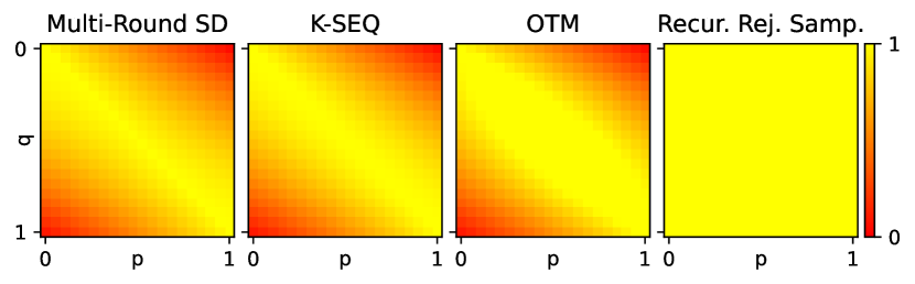
Toy example. We present a didactic example with Bernoulli distributions (given by Sun et al. (2023)) to showcase the benefit of recursive rejection sampling. Suppose that Bernoulli distributions are used for both draft and target models and only $K=2$ tokens are allowed for draft proposals. The acceptance rates for different methods are depicted in Figure 1; multi-round speculative decoding (from SpecInfer (Miao et al., 2023)), K-SEQ and Optimal Transport with Membership costs (OTM) (Sun et al., 2023), use sampling with replacement, whereas recursive rejection sampling uses sampling without replacement; note that both K-SEQ and OTM were presented in SpecTr paper (Sun et al., 2023) where OTM shows theoretically optimal acceptance rate. For all the baselines, acceptance rates decrease as the discrepancy between draft and target distribution increases, since tokens sampled from draft models become more unlikely from target models. On the other hand, recursive rejection sampling achieves 100% acceptance rate even with high draft-target-model discrepancy; once the first draft token is rejected, the second draft token is always aligned with the residual distribution. This example shows that draft distributions with dependencies, e.g., sampling-without-replacement distribution, leads to higher acceptance rate and becomes crucial, especially for the cases with higher distributional discrepancy between draft and target.

3.2 Tree-Based Speculative Decoding with Recursive Rejection Sampling

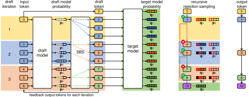
Recursive rejection sampling is applicable to tree-based speculative decoding algorithms if sampling without replacement is used to construct a draft-token tree. Two Recursive Speculative Decoding (RSD) algorithms using recursive rejection sampling are presented in this section, while they share the same pipeline for parallel target evaluation and draft tree verification after building the draft-token tree (See Figure 2.). We describe details about how RSD works in the following sections.

3.2.1 Draft-token tree generation

We consider two RSD algorithms: RSD with Constant branching factors (RSD-C) and RSD with Stochastic Beam Search (RSD-S). RSD-C builds the draft-token tree having constant branching factors, which makes sequences from the tree to have the same length. RSD-S, on the other hand, builds the tree via Stochastic Beam Search (Kool et al., 2019) that samples draft sequences without replacement, while truncating sequences that are unlikely to be generated from the draft model and efficiently handling the computational cost.

RSD with Constant branching factors (RSD-C). Let $L$ denote the fixed length for all draft sequences, which is equivalent to the depth of the draft-token tree, and $\boldsymbol{\tau}_{0}^{(1)}$ denote the input sequence of tokens. Let us assume that the tree level increases from root ($l=0$) to leaf ($l=L$) nodes, where each node is characterized by the (partial) sequence. We also define $\mathbf{b}:=(b_{0},...,b_{L-1})$ where $b_{l}$ is the branching factor at the level $l$ (See Figure 3(a) for the example with $\mathbf{b}=(3,2,1)$.).

At each level $l\in\{0,...,L-1\}$ of the draft tree, we begin with $N_{l}$ sequences $\boldsymbol{\tau}_{l}^{(k)},k=1,...,N_{l}$ generated from the previous level, where $N_{0}:=1$ and $N_{l}:=\prod_{l^{\prime}=0}^{l-1}b_{l^{\prime}}$ for $l\geq 1$. Then, we evaluate log probabilities $\phi_{l}(\boldsymbol{\tau}_{l}^{(k)},\cdot)$ and perturbed log probabilities $\tilde{\phi}_{l}(\boldsymbol{\tau}_{l}^{(k)},\cdot)$ for each $k$, i.e., for i.i.d. Gumbel samples $G_{l}^{(k)}(x),x\in\mathcal{X},$

$$\phi_{l}(\boldsymbol{\tau}_{l}^{(k)},\cdot) :=\log p(\cdot|\boldsymbol{\tau}_{l}^{(k)}),$$ (5)

$$\tilde{\phi}_{l}(\boldsymbol{\tau}_{l}^{(k)},\cdot) :=\phi_{l}(\boldsymbol{\tau}_{l}^{(k)},\cdot)+G_{l}^{(k)},$$ (6)

where both log probabilities and Gumbel samples can be computed in parallel; proper positional encodings and attention masking (Cai et al., 2023; Miao et al., 2023) are required for the parallel log-probability computation when transformer architecture is used (Vaswani et al., 2017). By using Gumbel-Top-$k$ trick (Vieira, 2014; Kool et al., 2019) with perturbed log probabilities (6), one can sample top-$b_{l}$ tokens without replacement for each sequence $\tau_{l}^{(k)}$:

$$\hat{X}_{l+1}^{((k-1)b_{l}+1)},...,\hat{X}_{l+1}^{((k-1)b_{l}+b_{l})}=\underset{x\in\mathcal{X}}{\mathrm{argtop}\text{-}b_{l}}\left(\tilde{\phi}_{l}(\boldsymbol{\tau}_{l}^{(k)},x)\right).$$ (7)

Note that the outputs $\hat{X}_{l+1}^{((k-1)b_{l}+k^{\prime})},k^{\prime}=1,...,b_{l},$ in (7) are assumed to be in the decreasing order of values $\tilde{\phi}_{l}(\boldsymbol{\tau}_{l}^{(k)},\hat{X}_{l+1}^{((k-1)b_{l}+k^{\prime})})$, for each $k$. Finally, we define

$$O_{l+1}^{((k-1)b_{l}+k^{\prime})} :=(\hat{X}_{l+1}^{((k-1)b_{l}+k^{\prime})},k),$$ (8)

$$\boldsymbol{\tau}_{l+1}^{((k-1)b_{l}+1)} :=(\boldsymbol{\tau}_{l}^{(k)},\hat{X}_{l+1}^{((k-1)b_{l}+1)})$$ (9)

for $k\in{1,...,N_{l}}$ and $k^{\prime}\in\{1,...,b_{l}\}$, where $O_{l+1}^{((k-1)b_{l}+k^{\prime})}$ is a pair of draft token and parent sequence index. Those pairs in (8) are stored for all levels $l=0,...,L-1$ and used for draft tree verification, which exploits the fact that the tokens $\hat{X}_{l+1}^{((k-1)b_{l}+1)},...,\hat{X}_{l+1}^{((k-1)b_{l}+b_{l})}$ follow sampling without replacement from $p(\cdot|\boldsymbol{\tau}_{l}^{(k)})$ for any given parent sequence index $k$.

Figure 3: We describe examples of constructing draft-token trees with the (maximum) draft length equal to 3; (a) The tree constructed by RSD-C with branching factors $\mathbf{b}=(3,2,1)$ is given; (b) we depict the tree constructed by RSD-S with beamwidth $W=3$, where edges are determined via Stochastic Beam Search.

RSD with Stochastic Beam Search (RSD-S). One caveat of RSD-C is that its constant branching factors $\mathbf{b}$ should be carefully determined to handle tree complexity, when the computation budget is limited; for example, if $\mathbf{b}=(n,...,n)$ with its length $L$, the number of nodes in the draft tree will be $\sum_{l=0}^{L-1}n^{l}=O(n^{L-1})$, which is computationally prohibitive for large $n$ and $L$. Also, RSD-C constructs sequences at each level $l$ by using the myopic token-wise log probabilities $\phi_{l}$ in (6). RSD-S addresses both issues by using Stochastic Beam Search (Kool et al., 2019) that early-truncates unlikely sequences and utilizes far-sighted sequence log probabilities.

Let us define the maximum draft sequence length $L$ and the beamwidth $W$. We also define $\boldsymbol{\tau}_{0}^{(1)}$ as the input sequence similar to RSD-C. At each level $l\in\{0,...,L-1\}$, SBS uses beam

$$\mathcal{B}_{l} :=(t_{l}^{(1)},...,t_{l}^{(W)}),$$

$$t_{l}^{(k)} :=(\boldsymbol{\tau}_{l}^{(k)},\phi_{l-1}(\boldsymbol{\tau}_{l}^{(k)}),\psi_{l-1}(\boldsymbol{\tau}_{l}^{(k)}))$$

generated from the previous level $l-1$. Here, each tuple $t_{l}^{(k)}$ for $k\in\{1,...,W\}$ consists of (a) a sequence $\boldsymbol{\tau}_{l}^{(k)}$, (b) its sequence log probability $\phi_{l-1}(\boldsymbol{\tau}_{l}^{(k)})$ of $\boldsymbol{\tau}_{l}^{(k)}$, and (c) the transformed (perturbed and truncated) sequence log probability $\psi_{l-1}(\boldsymbol{\tau}_{l}^{(k)})$, respectively.

For each tuple $t_{l}^{(k)}$ in the beam $\mathcal{B}_{l}$, we evaluate the (next-level) sequence log probabilities $\phi_{l}(\boldsymbol{\tau}_{l}^{(k)},\cdot)$ and the perturbed sequence log probabilities $\tilde{\phi}_{l}(\boldsymbol{\tau}_{l}^{(k)},\cdot)$. Specifically for i.i.d. Gumbel samples $G_{l}^{(k)}(x),x\in\mathcal{X}$, we compute

$$\phi_{l}(\boldsymbol{\tau}_{l}^{(k)},\cdot) :={\color[rgb]{1,0,0}\definecolor[named]{pgfstrokecolor}{rgb}{1,0,0}\phi_{l-1}(\boldsymbol{\tau}_{l}^{(k)})}+\log p(\cdot|{\color[rgb]{1,0,0}\definecolor[named]{pgfstrokecolor}{rgb}{1,0,0}\boldsymbol{\tau}_{l}^{(k)}}),$$

$$\tilde{\phi}_{l}(\boldsymbol{\tau}_{l}^{(k)},\cdot) :=\phi_{l}(\boldsymbol{\tau}_{l}^{(k)},\cdot)+G_{l}^{(k)},$$

where the terms $\boldsymbol{\tau}_{l}^{(k)}$ and $\phi_{l-1}(\boldsymbol{\tau}_{l}^{(k)})$ within the tuple $t_{l}^{(k)}$ of within the beam $\mathcal{B}_{l}$ are reused. Similar to RSD-C, both log probabilities and Gumbel samples can be parallelly computed with positional encodings and attention masking (Cai et al., 2023; Miao et al., 2023). In addition to the perturbed log probabilities, SBS in RSD-S transforms $\tilde{\phi}_{l}(\boldsymbol{\tau}_{l}^{(k)},\cdot)$ into the truncated function

$$\psi_{l}(\boldsymbol{\tau}_{l}^{(k)},\cdot) :=T({\color[rgb]{1,0,0}\definecolor[named]{pgfstrokecolor}{rgb}{1,0,0}\psi_{l-1}(\boldsymbol{\tau}_{l}^{(k)})},\tilde{\phi}_{l}(\boldsymbol{\tau}_{l}^{(k)},\cdot)),$$ (10)

$$T(u,\phi) :=-\log\left(e^{-u}-e^{-\mathrm{max}\phi}+e^{-\phi(\cdot)}\right)$$ (11)

for $\max\phi:=\max_{x\in\mathcal{X}}\phi(x)$ by reusing $\psi_{l-1}(\boldsymbol{\tau}_{l}^{(k)})$ in $t_{l}^{(k)}$ . Note that $T(u,\phi)$ in (11) is monotonically increasing w.r.t. $\phi$ and transforms $\phi$ to the function with the upper bound $u$ (Kool et al., 2019)

After evaluating $\psi_{l}(\boldsymbol{\tau}_{l}^{(k)},\cdot)$ for all parent sequences $\boldsymbol{\tau}_{l}^{(k)}$s, SBS selects top-$W$ pairs $(\hat{X}_{l+1},p_{l+1})$ of draft token and parent sequence index across the beam $\mathcal{B}_{l}$, i.e.,

$$O_{l+1}^{(1)},...,O_{l+1}^{(W)}:=\underset{(x,k)\in\mathcal{X}\times\mathcal{K}}{\mathrm{argtop}\text{-}W}\left(\psi_{l}(\boldsymbol{\tau}_{l}^{(k)},x)\right)$$ (12)

for $O_{l+1}^{(k)}:=(\hat{X}_{l+1}^{(k)},p_{l+1}^{(k)})$ and $\mathcal{K}:=\{1,...,W\}$. The output pairs $O_{l+1}^{(1)},...,O_{l+1}^{(W)}$ are given by corresponding values $\psi_{l}(\boldsymbol{\tau}_{l}^{(k)},\hat{X}_{l+1}^{(k)})$ in the decreasing order. Finally, we construct the next beam

$$\mathcal{B}_{l+1} :=(t_{l+1}^{(1)},...,t_{l+1}^{(W)}),$$

$$t_{l+1}^{(k)} :=((\hat{\boldsymbol{\tau}}_{l+1}^{(k)},\hat{X}_{l+1}^{(k)}),\phi_{l}(\hat{\boldsymbol{\tau}}_{l+1}^{(k)},\hat{X}_{l+1}^{(k)}),\psi_{l}(\hat{\boldsymbol{\tau}}_{l+1}^{(k)},\hat{X}_{l+1}^{(k)}))$$

for $k=1,...,W$, where $\hat{\boldsymbol{\tau}}_{l+1}^{(k)}:=\boldsymbol{\tau}_{l}^{(p_{l+1}^{(k)})}$ is the selected parent sequence. Intuitively, SBS at the level $l$ evaluates scores $\psi_{l}^{(k)}(\boldsymbol{\tau}_{l}^{(k)},x),x\in\mathcal{X},k\in\mathcal{K},$ by considering all child nodes from the beam $\mathcal{B}_{l}$. SBS selects $W$ nodes among all child nodes having top-$W$ scores. Note that the above process is theoretically equivalent to sample top-$W$ length-$(l+1)$ sequences without replacement (Kool et al., 2019) and efficiently truncates sequences that are unlikely to be generated. (See Figure 3(b).)

We store the ordered sequence of pairs $O_{l+1}^{(1)},...,O_{l+1}^{(W)}$ for all levels $l=0,...,L-1$, which is used for draft-tree verification. As in RSD-C, we show the following property:

Theorem 3.2 (Tokens from the same sequence follow sampling without replacement in RSD-S).

In RSD-S, any non-empty subsequence of the sequence $\hat{X}_{l+1}^{(1)},...,\hat{X}_{l+1}^{(W)}$ of draft tokens (from $O_{l+1}^{(1)},...,O_{l+1}^{(W)}$ in (12)) such that each element of the subsequence has the same parent $\boldsymbol{\tau}_{l}^{(k)}$ follows sampling without replacement from $p(\cdot|\boldsymbol{\tau}_{l}^{(k)})$.

Proof.

See Appendix A.2. ∎

3.2.2 Draft-tree evaluation and verification

Tree evaluation with target model. After the draft-tree construction, we have sequences of pairs

$$(O_{l}^{(1)},...,O_{l}^{(N_{l})}),l=1,...,L,$$

where $N_{l}=\prod_{l^{\prime}=0}^{l}b_{l^{\prime}}$ for RSD-C and $N_{l}=W$ for RSD-S, respectively ($N_{0}:=1$ for both). Those pairs include the node-connection information of the draft tree and can be used to parallelly evaluate the draft tree via the target model by utilizing appropriate attention masking and positional encodings. From the evaluation process, we acquire the target log probabilities for all sequences $\boldsymbol{\tau}_{l}^{(k_{l})}$ in the draft tree, i.e.,

$$q(\cdot|\boldsymbol{\tau}_{l}^{(k_{l})}),l=0,...,L,k_{l}=1,...,N_{l}.$$

Verification via recursive rejection sampling. Earlier, we show that tokens in the tree having the same parent sequence $\boldsymbol{\tau}_{l}^{(k_{l})}$ follows the sampling-without-replacement distribution from $p(\cdot|\boldsymbol{\tau}_{l}^{(k_{l})})$ for both RSD-C and RSD-S. Thus, one can apply recursive rejection sampling iteratively at each tree level.

Specifically, at the level $l\in\{0,1,...,L\}$, we begin with a sequence $\boldsymbol{\tau}_{l}^{(k_{l}^{\prime})}$ where $k_{l}^{\prime}$ is the index of the parent sequence accepted in the previous level ($k_{0}^{\prime}=1$ at the level $l=0$). Within the ordered sequence $(O_{l+1}^{(1)},...,O_{l+1}^{(N_{l+1})})$ of pairs, we find the subsequence $\mathbf{o}_{l+1}^{(k_{l}^{\prime})}$ having $\boldsymbol{\tau}_{l}^{(k_{l}^{\prime})}$ as parent, which can be validated by checking the second element of each pair $O_{l+1}^{(k)}$, and the token sequence $\mathbf{x}_{l+1}^{(k_{l}^{\prime})}$ in $\mathbf{o}_{l+1}^{(k_{l}^{\prime})}$. Earlier, we show that tokens $\mathbf{x}_{l+1}^{(k_{l}^{\prime})}$ follows sampling-without-replacement distribution in its order, so we can apply recursive rejection sampling to those tokens with draft and target distributions, $p(\cdot|\boldsymbol{\tau}_{l}^{(k_{l}^{\prime})})$ and $q(\cdot|\boldsymbol{\tau}_{l}^{(k_{l}^{\prime})})$, respectively. If any token $x$ in $\mathbf{x}_{l+1}^{(k_{l}^{\prime})}$ is accepted, we set $k_{l+1}^{\prime}$ that corresponds to $\boldsymbol{\tau}_{l}^{(k_{l+1}^{\prime})}:=(\boldsymbol{\tau}_{l}^{(k_{l}^{\prime})},x)$, and we continue to the next-level verification if child nodes exist. If all tokens are rejected, we sample from the last residual distribution of recursiver rejection sampling. If there is no child node, we sample from the target $q(\cdot|\boldsymbol{\tau}_{l}^{(k_{l}^{\prime})})$ similar to the single-sequence speculative decoding (Chen et al., 2023; Leviathan et al., 2023). We provide detailed descriptions for RSD-C (Algorithm 2) and for RSD-S (Algorithm 7) in Appendix B.

Figure 4: Block efficiency, MBSU, token rate and accuracy for various lengths ($2,3,4,5$) of draft sequences are given. We consider two target models, Llama 2-70B and Llama 2-Chat-70B, each of which has a corresponding smaller draft model for speculative decoding. All results are normalized by the corresponding numbers from auto-regressive decoding. RSD-S always outperforms SD, SpecTr and RSD-C. All methods including auto-regressive decoding show similar accuracy for WMT and XSum.

Figure 5: Block efficiency, MBSU, token rate and accuracy for various target computational budgets (the numbers $6,10,14,21,30$ of draft tokens processed at the target model) are given. We consider two target models, Llama 2-70B and Llama 2-Chat-70B, each of which has a corresponding smaller draft model for speculative decoding. All results are normalized by the corresponding numbers from auto-regressive decoding. RSD-S outperforms SD, SpecTr and RSD-C in the majority of cases. All methods including auto-regressive decoding show similar accuracy for both WMT and XSum.

4 Related Works

Many recent works have aimed to address the inference bottleneck of LLMs caused by auto-regressive decoding. Speculative decoding methods (Leviathan et al., 2023; Chen et al., 2023; Sun et al., 2023; Miao et al., 2023) use the target model (LLM) with a draft model (a small language model), while recovering target distribution via rejection sampling. See the recent survey on speculative decoding (Xia et al., 2024) for more comprehensive understanding.

Other than speculative decoding methods, BiLD (Kim et al., 2023) is another method to accelerate inference, where it uses a fallback policy which determines when to invoke the target model and a rollback policy to review and correct draft tokens. Medusa (Cai et al., 2024) uses multiple decoding heads to predict future tokens in parallel, constructs the draft-token tree and uses a typical acceptance criteria. Lookahead decoding (Fu et al., 2023) caches the historical $n$-grams generated on-the-fly instead of having a draft model and performs parallel decoding using Jacobi iteration and verifies $n$-grams from the cache. While showing promising results with greedy sampling, these works do not guarantee target distribution recovery in contrast to speculative decoding methods.

5 Experiments

We evaluate RSD-C and RSD-S together with our baselines including speculative decoding (SD) (Chen et al., 2023; Leviathan et al., 2023) and SpecTr (Sun et al., 2023), where a single draft model is assumed. We consider the following perspectives during our experiments: (Exp1) How will the performance be affected by the length of draft sequences? (Exp2) How will the performance be affected by the target computational budget, i.e., the number of tokens processed at the target model? While (Exp1) has been frequently investigated by existing tree-based speculative decoding methods (Sun et al., 2023; Miao et al., 2023), (Exp2) has not been considered in prior works but has practical importance when running the target model on resource-bounded devices.
Models. We consider the following target models; Llama 2 and Llama 2-Chat (Touvron et al., 2023) with 7B, 13B and 70B parameters; OPT (Zhang et al., 2022) with 13B, 30B and 66B parameters. Each class of target models adopts corresponding draft model; see Appendix C.1. In this section, we only present Llama 2-70B and Llama 2-Chat-70B results, and other results (Llama 2 with other sizes and OPT) can be found in Appendix C.4.
Tasks. Our methods and baselines are evaluated for WMT18-DeEn (Bojar et al., 2018, translation) and XSum (Narayan et al., 2018, summarization) for each target model, while we report accuracy scores (BLEU for WMT and ROUGE-2 for XSum) to confirm if the target model’s distribution is recovered; Databricks-Dolly-15k (Conover et al., 2023, question and answering) is used only for Llama 2-Chat without accuracy evaluation. We use temperature 0.3 for both XSum and WMT and 1.0 for Dolly, where we further apply nucleus (top-$p$) sampling (Holtzman et al., 2019) with $p=0.95$ for Dolly.
Performance metrics. We evaluate block efficiency (Leviathan et al., 2023), Memory-Bound Speed-Up (MBSU) (Zhou et al., 2023) and token rate (tokens/sec) on A100 GPUs; see Appendix C.2 for details.

5.1 (Exp 1) Fixed draft sequence length

We fix (maximum) draft sequence length as the value in $\{2,3,4,5\}$ and evaluate our methods and baselines, which is summarized in Figure 4. Regarding the tree structures of each decoding methods, we let both SpecTr and RSD-S always use draft-token trees, the size of which is smaller than or equal to that of RSD-C’s tree; see Appendix C.3.1 for details. Our results show that tree-based methods (SpecTr, RSD-C and RSD-S) always outperform SD in terms of block efficiency and MBSU, whereas token rates for SpecTr and RSD-C can be lower than that for SD; this is since block efficiencies for both SpecTr and RSD-C are relatively low and there is additional computational overhead to process the tree. On the other hand, RSD-S strictly outperforms both SD and SpecTr for all performance metrics, showing the superiority of RSD-S over our baselines and the importance of early-truncating unlikely draft sequences. We also observe that there is no strong correlation between MBSU and token rate; this is since A100 GPUs used to measure token rates are not memory-bound. Furthermore, token rates in many cases are shown to decrease as the length of draft-token sequence becomes higher, which is due to the increased computation overhead to execute draft models with the longer draft sequence; however, one needs to be cautious since this result may not generally hold since token rate is hugely affected by the efficiency of software implementation and the devices which we execute the methods on. Finally, in WMT and XSum, BLEU and ROUGE-2 scores are similar across different methods, respectively, which implies that all methods recover the distributions of target LLMs.

5.2 (Exp2) Fixed target computational budget

We select target computational budget, i.e., the number of draft tokens processed at the target model in parallel for each speculative decoding iteration, among values in $\{6,10,14,21,30\}$ and evaluate our proposed methods and baselines; we summarize the results in Figure 5 and describe tree structures in Appendix C.3.2. While RSD-S achieves higher block efficiency and MBSU than SD and SpecTr in most cases, SD beats RSD-C in the relatively low budget regime $\{6,10,14\}$ in XSum experiments, when using Llama 2-70B as a target model. We believe that our draft model is well-aligned with Llama 2-70B in XSum task (from the observation that block efficiency between 2.4 and 3.0, which is significantly higher than the numbers in other cases, is achieved), and increasing the depth rather than the width of the tree could quickly increase the acceptance rate in this case. In the high budget regime ($\{21,30\}$), on the other hand, RSD-S beats SD for both block efficiency and MBSU. In terms of token rate, RSD-S strictly outperforms our baselines, whereas SD’s token rate severely decreases for higher target computation budgets due to the computational overhead caused by the draft model’s auto-regressive decoding with the longer draft sequence.

6 Conclusion

We present RSD algorithms, a novel tree-based speculative decoding method leveraging the full diversifiability of the draft-token tree; RSD-C efficiently samples draft tokens without replacement via Gumbel-Top-$k$ trick, while RSD-S uses Stochastic Beam Search and samples draft-token sequences without replacement. We also propose recursive rejection sampling that can verify the tree built by the sampling-without-replacement process and recovers the exact target model distribution. We show that RSD outperforms the baselines in most cases, supporting the importance of diverse drafting when accelerating LLM inference.

Appendix A Theorems and proofs

A.1 Proof of Theorem 3.1

Theorem 3.1 (Recursive rejection sampling recovers target distribution).

The random variable $Z\in\mathcal{X}$ defining recursive rejection sampling rule (4) follows the target distribution $q$, i.e.,

$$\mathrm{Pr}\left\{Z=z\right\}=q(z),z\in\mathcal{X}.$$

Proof.

We remain a sketch of the proof here and the formal proof is given in the next paragraph. We first consider the case where $\hat{X}^{(1)},...,\hat{X}^{(K-1)}$ are rejected and see whether we accept $\hat{X}^{(K)}$ or not; we either accept $\hat{X}^{(K)}$ with probability $\Theta^{(K)}$ in (3) or sample a new token $Y\sim q^{(K+1)}(\cdot|\hat{X}^{(1:K-1)})$ when all draft tokens are rejected. Since $q^{(K+1)}$ is the residual distribution from $q^{(K)}$, one can regard it as the simple sampling by Chen et al. (2023) and Leviathan et al. (2023), which recovers $q^{(K)}$. The same idea is applied to $\hat{X}^{(K-1)},...,\hat{X}^{(1)}$ in the reversed order until we recover $q=q^{(1)}$ at the end.

Let us desribe the formal proof. From the definition of recursive rejection sampling (4), we have

$$\mathrm{Pr}\left\{Z=z\right\}=\sum_{k=1}^{K}\underbrace{\mathrm{Pr}\left\{A^{(1:k-1)}=\mathtt{rej}^{k-1},\hat{X}^{(k)}=z,A^{(k)}=\mathtt{acc}\right\}}_{=:\Sigma_{1,k}}+\underbrace{\mathrm{Pr}\left\{A^{(1:K)}=\mathtt{rej}^{K},\tilde{X}^{(K+1)}=z\right\}}_{=:\Sigma_{2,K}}.$$

It can be shown that the following equality holds for each $k$:

$$\Sigma_{2,k-1}=\Sigma_{1,k}+\Sigma_{2,k}.$$ (13)

Let us first consider $k=K$, then,

$$\Sigma_{1,K}+\Sigma_{2,K}$$

$$=\sum_{x^{(1)},...,x^{(K-1)}}\mathrm{Pr}\left\{\hat{X}^{(1:K-1)}=x^{(1:K-1)}\right\}\times\mathrm{Pr}\left\{A^{(1:K-1)}=\mathtt{rej}^{K-1},\hat{X}^{(K)}=z,A^{(K)}=\mathtt{acc}\bigg{|}\hat{X}^{(1:K-1)}=x^{(1:K-1)}\right\}$$

$$+\sum_{x^{(1)},...,x^{(K)}}\mathrm{Pr}\left\{\hat{X}^{(1:K)}=x^{(1:K)}\right\}\times\mathrm{Pr}\left\{A^{(1:K)}=\mathtt{rej}^{K},\hat{X}^{(K+1)}=z\bigg{|}\hat{X}^{(1:K)}=x^{(1:K)}\right\}$$

$$=\sum_{x^{(1)},...,x^{(K-1)}}\mathrm{Pr}\left\{\hat{X}^{(1:K-1)}=x^{(1:K-1)}\right\}\Bigg{(}\underbrace{\mathrm{Pr}\left\{A^{(1:K-1)}=\mathtt{rej}^{K-1},\hat{X}^{(K)}=z,A^{(K)}=\mathtt{acc}\bigg{|}\hat{X}^{(1:K-1)}=x^{(1:K-1)}\right\}}_{=:T_{1}(K)}$$

$$~{}~{}~{}~{}~{}~{}~{}~{}~{}~{}~{}~{}~{}~{}~{}~{}~{}~{}~{}~{}~{}~{}~{}~{}~{}+\underbrace{\sum_{x^{(K)}}\mathrm{Pr}\left\{\hat{X}^{(K)}=x^{(K)}\bigg{|}\hat{X}^{(1:K-1)}=x^{(1:K-1)}\right\}\times\mathrm{Pr}\left\{A^{(1:K)}=\mathtt{rej}^{K},\hat{X}^{(K+1)}=z\bigg{|}\hat{X}^{(1:K)}=x^{(1:K)}\right\}}_{=:T_{2}(K)}\Bigg{)}.$$

One can represent $T_{1,K}$ and $T_{2,K}$ as follows:

$$T_{1,K} =\mathrm{Pr}\left\{A^{(1:K-1)}=\mathtt{rej}^{K-1}\bigg{|}\hat{X}^{(1:K-1)}=x^{(1:K-1)}\right\}$$

$$~{}~{}~{}~{}~{}\times\mathrm{Pr}\left\{\hat{X}^{(K)}=z\bigg{|}\hat{X}^{(1:K-1)}=x^{(1:K-1)}\right\}\times\mathrm{Pr}\left\{A^{(K)}=\mathtt{acc}\Bigg{|}\hat{X}^{(1:K)}=(x^{(1:K-1)},z)\right\}$$

$$=\mathrm{Pr}\left\{A^{(1:K-1)}=\mathtt{rej}^{K-1}\bigg{|}\hat{X}^{(1:K-1)}=x^{(1:K-1)}\right\}p^{(K)}(z|x^{(1:K-1)})\min\left\{1,\frac{q^{(K)}(z|x^{(1:K-2)})}{p^{(K)}(z|x^{(1:K-1)})}\right\}$$

$$=\mathrm{Pr}\left\{A^{(1:K-1)}=\mathtt{rej}^{K-1}\bigg{|}\hat{X}^{(1:K-1)}=x^{(1:K-1)}\right\}\min\left\{p^{(K)}(z|x^{(1:K-1)}),q^{(K)}(z|x^{(1:K-2)})\right\},$$

$$T_{2,K} =\sum_{x^{(K)}}\mathrm{Pr}\left\{\hat{X}^{(K)}=x^{(K)}\bigg{|}\hat{X}^{(1:K-1)}=x^{(1:K-1)}\right\}\times\mathrm{Pr}\left\{A^{(1:K)}=\mathtt{rej}^{K},\hat{X}^{(K+1)}=z\bigg{|}\hat{X}^{(1:K)}=x^{(1:K)}\right\}$$

$$=\sum_{x^{(K)}}p^{(K)}(x^{(K)}|x^{(1:K-1)})\times\mathrm{Pr}\left\{A^{(1:K)}=\mathtt{rej}^{K}\bigg{|}\hat{X}^{(1:K)}=x^{(1:K)}\right\}\times\mathrm{Pr}\left\{\hat{X}^{(K+1)}=z\bigg{|}\hat{X}^{(1:K)}=x^{(1:K)}\right\}$$

$$=\sum_{x^{(K)}}p^{(K)}(x^{(K)}|x^{(1:K-1)})\times\mathrm{Pr}\left\{A^{(1:K)}=\mathtt{rej}^{K}\bigg{|}\hat{X}^{(1:K)}=x^{(1:K)}\right\}\times q^{(K+1)}(z|x^{(1:K-1)})$$

$$=\sum_{x^{(K)}}p^{(K)}(x^{(K)}|x^{(1:K-1)})\times\mathrm{Pr}\left\{A^{(1:K-1)}=\mathtt{rej}^{K-1}\bigg{|}\hat{X}^{(1:K-1)}=x^{(1:K-1)}\right\}$$

$$~{}~{}~{}~{}~{}~{}~{}~{}~{}~{}\times\mathrm{Pr}\left\{A^{(K)}=\mathtt{rej}\bigg{|}\hat{X}^{(1:K)}=x^{(1:K)}\right\}\times q^{(K+1)}(z|x^{(1:K-1)})$$

$$=\mathrm{Pr}\left\{A^{(1:K-1)}=\mathtt{rej}^{K-1}\bigg{|}\hat{X}^{(1:K-1)}=x^{(1:K-1)}\right\}q^{(K+1)}(z|x^{(1:K-1)})$$

$$~{}~{}~{}~{}~{}~{}~{}~{}~{}~{}\times\sum_{x^{(K)}}p^{(K)}(x^{(K)}|x^{(1:K-1)})\times\mathrm{Pr}\left\{A^{(K)}=\mathtt{rej}\bigg{|}\hat{X}^{(1:K)}=x^{(1:K)}\right\}$$

$$=\mathrm{Pr}\left\{A^{(1:K-1)}=\mathtt{rej}^{K-1}\bigg{|}\hat{X}^{(1:K-1)}=x^{(1:K-1)}\right\}q^{(K+1)}(z|x^{(1:K-1)})$$

$$~{}~{}~{}~{}~{}~{}~{}~{}~{}~{}\times\sum_{x^{(K)}}p^{(K)}(x^{(K)}|x^{(1:K-1)})\times\left(1-\mathrm{Pr}\left\{A^{(K)}=\mathtt{acc}\bigg{|}\hat{X}^{(1:K)}=x^{(1:K)}\right\}\right)$$

$$=\mathrm{Pr}\left\{A^{(1:K-1)}=\mathtt{rej}^{K-1}\bigg{|}\hat{X}^{(1:K-1)}=x^{(1:K-1)}\right\}q^{(K+1)}(z|x^{(1:K-1)})$$

$$~{}~{}~{}~{}~{}~{}~{}~{}~{}~{}\times\sum_{x^{(K)}}p^{(K)}(x^{(K)}|x^{(1:K-1)})\times\left(1-\min\left\{1,\frac{q^{(K)}(x^{(K)}|x^{(1:K-2)})}{p^{(K)}(x^{(K)}|x^{(1:K-1)})}\right\}\right)$$

$$=\mathrm{Pr}\left\{A^{(1:K-1)}=\mathtt{rej}^{K-1}\bigg{|}\hat{X}^{(1:K-1)}=x^{(1:K-1)}\right\}\frac{\max\left\{0,q^{(K)}(z|x^{(1:K-2)})-p^{(K)}(z|x^{(1:K-1)})\right\}}{\sum_{x^{(K)}}\max\left\{0,q^{(K)}(x^{(k)}|x^{(1:K-2)})-p^{(K)}(x^{(K)}|x^{(1:K-1)})\right\}}$$

$$~{}~{}~{}~{}~{}~{}~{}~{}~{}~{}\times\sum_{x^{(K)}}\max\left\{0,q^{(K)}(x^{(K)}|x^{(1:K-2)})-p^{(K)}(x^{(K)}|x^{(1:K-1)})\right\}$$

$$=\mathrm{Pr}\left\{A^{(1:K-1)}=\mathtt{rej}^{K-1}\bigg{|}\hat{X}^{(1:K-1)}=x^{(1:K-1)}\right\}\max\left\{0,q^{(K)}(z|x^{(1:K-2)})-p^{(K)}(z|x^{(1:K-1)})\right\}.$$

Therefore, we have

$$T_{1,K}+T_{2,K}$$

$$=\mathrm{Pr}\left\{A^{(1:K-1)}=\mathtt{rej}^{K-1}\bigg{|}\hat{X}^{(1:K-1)}=x^{(1:K-1)}\right\}$$

$$~{}~{}~{}~{}~{}~{}~{}~{}~{}~{}\times\left(\min\left\{p^{(K)}(z|x^{(1:K-1)}),q^{(K)}(z|x^{(1:K-2)})\right\}+\max\left\{0,q^{(K)}(z|x^{(1:K-2)})-p^{(K)}(z|x^{(1:K-1)})\right\}\right)$$

$$=\mathrm{Pr}\left\{A^{(1:K-1)}=\mathtt{rej}^{K-1}\bigg{|}\hat{X}^{(1:K-1)}=x^{(1:K-1)}\right\}q^{(K)}(z|x^{(1:K-2)})$$

$$=\mathrm{Pr}\left\{A^{(1:K-1)}=\mathtt{rej}^{K-1},\tilde{X}^{(K)}=z\bigg{|}\hat{X}^{(1:K-1)}=x^{(1:K-1)}\right\},$$

where we define a random variable $\tilde{X}^{(K)}$ such that

$$\mathrm{Pr}\left\{\tilde{X}^{(K)}=z\bigg{|}\hat{X}^{(1:K-1)}=x^{(1:K-1)}\right\}:=q^{(K)}(z|x^{(1:K-1)}),$$

which leads to

$$\Sigma_{1,K}+\Sigma_{2,K}$$

$$=\sum_{x^{(1)},...,x^{(K-1)}}\mathrm{Pr}\left\{\hat{X}^{(1:K-1)}=x^{(1:K-1)}\right\}(T_{1,K}+T_{2,K})$$

$$=\sum_{x^{(1)},...,x^{(K-1)}}\mathrm{Pr}\left\{\hat{X}^{(1:K-1)}=x^{(1:K-1)}\right\}\times\mathrm{Pr}\left\{A^{(1:K-1)}=\mathtt{rej}^{K-1},\tilde{X}^{(K)}=z\bigg{|}\hat{X}^{(1:K-1)}=x^{(1:K-1)}\right\}$$

$$=\mathrm{Pr}\left\{A^{(1:K-1)}=\mathtt{rej}^{K-1},\tilde{X}^{(K)}=z\right\}$$

$$=\Sigma_{2,K-1}.$$

Since the same derivation can be done for $k=2,...,K-1$, we have

$$\mathrm{Pr}\left\{Z=z\right\}=\sum_{k=1}^{K}\Sigma_{1,k}+\Sigma_{2,K}=\sum_{k=1}^{K-1}\Sigma_{1,k}+\Sigma_{2,K-1}=\cdots=\Sigma_{1,1}+\Sigma_{2,1}=q(z),$$

where the last equality holds from the derivation of original speculative decoding by (Chen et al., 2023; Leviathan et al., 2023). ∎

A.2 Proof of Theorem 3.2

Theorem 3.2 (Tokens from the same sequence follow sampling without replacement in RSD-S).

In RSD-S, any non-empty subsequence of the sequence $\hat{X}_{l+1}^{(1)},...,\hat{X}_{l+1}^{(W)}$ of draft tokens (from $O_{l+1}^{(1)},...,O_{l+1}^{(W)}$ in (12)) such that each element of the subsequence has the same parent $\boldsymbol{\tau}_{l}^{(k)}$ follows sampling without replacement from $p(\cdot|\boldsymbol{\tau}_{l}^{(k)})$.

Proof.

For fixed $\boldsymbol{\tau}_{l}^{(k)}$, consider a sequence of tokens

$$\bar{\mathbf{X}}_{l+1}^{(k)}:=\underset{x\in\mathcal{X}}{\mathrm{argsort}}~{}\psi_{l}(\boldsymbol{\tau}_{l}^{(k)},x)=\underset{x\in\mathcal{X}}{\mathrm{argsort}}~{}\tilde{\phi}_{l}(\boldsymbol{\tau}_{l}^{(k)},x),$$

where the last equality holds since $T$ in (10) is monotonically increasing w.r.t. $\tilde{\phi}_{l}(\boldsymbol{\tau}_{l}^{(k)},\cdot)$ for fixed $\boldsymbol{\tau}_{l}^{(k)}$. Thus, $\bar{\mathbf{X}}_{l+1}^{(k)}$ can be seen as samples from $p(\cdot|\boldsymbol{\tau}_{l}^{(k)})$ without replacement.

For a length-$l_{k}$ subsequence $\mathbf{o}_{l+1}^{(k)}$ of $(O_{l+1}^{(1)},...,O_{l+1}^{(W)})$ in (12), where each element of the subsequence have $\boldsymbol{\tau}_{l}^{(k)}$ as its parent, the token sequence in $\mathbf{o}_{l+1}^{(k)}$ is a subsequence of $\bar{\mathbf{X}}_{l+1}^{(k)}$, i.e., those tokens are top-$l_{k}$ samples without replacement from $p(\cdot|\boldsymbol{\tau}_{l}^{(k)})$. ∎

Appendix B Algorithm

B.1 Recursive Speculative Decoding with Constant Branching Factors (RSD-C)

Algorithm 2 Recursive Speculative Decoding with Constant Branching Factors (RSD-C)

1:  Input: The length $L_{\mathrm{draft}}$ of draft sequences (depth of the draft tree), a sequence $\mathbf{x}_{\mathrm{input}}$ of input tokens, a list $\mathbf{b}:=[b_{0},...,b_{L_{\mathrm{draft}}-1}]$ of constant branching factors in the draft tree, the maximum length $L_{\mathrm{output}}$ of the output sequence.

2:  // Get the length of the input sequence. $L_{\mathrm{input}}\leftarrow\mathtt{GetLength}(\mathbf{x}_{\mathrm{input}})$.

3:  // Initialize empty KV caches for draft and target models. $\mathbf{C}_{\mathrm{draft}}\leftarrow\emptyset$, $\mathbf{C}_{\mathrm{target}}\leftarrow\emptyset$.

4:  while $L_{\mathrm{input}}<L_{\mathrm{output}}$ do

5:     // (STEP 1) Create a draft tree by using the draft model. $\mathcal{T},\mathbf{x}_{\mathrm{input}},\mathbf{C}_{\mathrm{draft}},\mathbf{M},\mathbf{id}_{\mathrm{position}},\mathcal{L}_{\mathrm{num\_nodes}}\leftarrow\mathtt{CreateDraftTreeConst}(\mathbf{x}_{\mathrm{input}},\mathbf{C}_{\mathrm{draft}},\mathbf{b},L_{\mathrm{draft}}).$

6:     // (STEP 2) Evaluate draft tokens by using the target model. // - Apply $\mathbf{M}$ to the right below corner of attention weights. // - The target log probability $\boldsymbol{\Phi}_{\mathrm{target}}$ is a $\mathtt{GetLength}(\mathbf{x}_{\mathrm{input}})\times N_{\mathrm{vocab}}$ tensor. // - $N_{\mathrm{vocab}}$ is the vocabulary size. $\boldsymbol{\Phi}_{\mathrm{target}},\mathbf{C}_{\mathrm{target}}\leftarrow\mathtt{TargetModelForwardPass}(\mathbf{x}_{\mathrm{input}},\mathbf{C}_{\mathrm{target}},\mathbf{id}_{\mathrm{position}},\mathbf{M})$.

7:     // - Convert the log probability tensor into the list of log probabilities for each level of the tree. $\mathcal{L}_{\mathrm{log\_probs\_target}}\leftarrow\mathtt{SplitTensor}(\boldsymbol{\Phi}_{\mathrm{target}}[-\mathtt{Sum}(\mathcal{L}_{\mathrm{num\_nodes}}):,:],\mathcal{L}_{\mathrm{num\_nodes}},\mathtt{dim}=0)$

8:     // (STEP 3) Run Recursive Rejection Sampling for each level of the tree. $\mathbf{x}_{\mathrm{accepted}},\mathbf{x}_{\mathrm{last}},\mathbf{id}_{\mathrm{accepted\_flat\_node}}\leftarrow\mathtt{RecursiveRejectionSampling}(\mathcal{T},\mathcal{L}_{\mathrm{log\_probs\_target}})$

9:     // (STEP 4) Use KV caches that are accepted, and prepare for the next round. $\mathbf{C}_{\mathrm{draft}},\mathbf{C}_{\mathrm{target}}\leftarrow\mathtt{FilterKVCache}(\mathbf{C}_{\mathrm{draft}},\mathbf{C}_{\mathrm{target}},L_{\mathrm{input}},\mathbf{id}_{\mathrm{accepted\_flat\_node}})$

10:     $\mathbf{x}_{\mathrm{input}}\leftarrow\mathtt{Concat}([\mathbf{x}_{\mathrm{input}}[:L_{\mathrm{input}}],\mathbf{x}_{\mathrm{accepted}},\mathbf{x}_{\mathrm{last}}])$

11:     $L_{\mathrm{input}}\leftarrow\mathtt{GetLength}(\mathbf{x}_{\mathrm{input}})$

12:  end while

13:  Output: a sequence $\mathbf{x}_{\mathrm{input}}$ that includes both input tokens and generated output tokens.

Algorithm 3 $\mathtt{CreateDraftTreeConst}(\mathbf{x}_{\mathrm{input}},\mathbf{C}_{\mathrm{draft}},\mathbf{b},L_{\mathrm{draft}})$

1:  Input: An input sequence $\mathbf{x}_{\mathrm{input}}$, the draft KV cache $\mathbf{C}_{\mathrm{draft}}$, the branching factor $\mathbf{b}:=[b_{0},...,b_{L_{\mathrm{draft}}-1}]$, the draft length $L_{\mathrm{draft}}$

2:  // Get the length of the input sequence. $L_{\mathrm{input}}\leftarrow\mathtt{GetLength}(\mathbf{x}_{\mathrm{input}})$.

3:  // Initialize lists for 1) draft log probabilities, 2) flattened node IDs, 3) parent node ids (within each level of the draft tree), 4) draft tokens, 5) numbers of nodes (for all levels of the tree), respectively. $\mathcal{L}_{\mathrm{log\_probs\_draft}}\leftarrow[~{}],\mathcal{L}_{\mathrm{flat\_node\_ids}}\leftarrow[~{}],\mathcal{L}_{\mathrm{parent\_ids}}\leftarrow[~{}],\mathcal{L}_{\mathrm{draft\_tokens}}\leftarrow[~{}],\mathcal{L}_{\mathrm{num\_nodes}}\leftarrow[~{}]$.

4:  // Initialize a draft tree. $\mathcal{T}\leftarrow(\mathcal{L}_{\mathrm{log\_probs\_draft}},\mathcal{L}_{\mathrm{flat\_node\_ids}},\mathcal{L}_{\mathrm{parent\_ids}},\mathcal{L}_{\mathrm{draft\_tokens}})$.

5:  // Set an empty attention mask, and position ids; inclusive for $\mathtt{start}$ and exclusive for $\mathtt{end}$. $\mathbf{M}\leftarrow\emptyset$, $\mathbf{id}_{\mathrm{position}}\leftarrow\mathtt{Arange}(\mathtt{start}=0,\mathtt{end}=L_{\mathrm{input}})$.

6:  // Set the counter to check the number of nodes in the tree. $N_{\mathrm{tree\_prev}}\leftarrow 0$, $N_{\mathrm{tree\_curr}}\leftarrow 0$.

7:  // Set the number of nodes at the current level of the tree. $N_{\mathrm{nodes}}\leftarrow 1$, $\mathcal{L}_{\mathrm{num\_nodes}}\mathtt{.append}(N_{\mathrm{nodes}})$.

8:  for $l_{\mathrm{draft}}=0$ to $L_{\mathrm{draft}}-1$ do

9:     // Apply $\mathbf{M}$ to the right below corner of attention weights. // The draft log probability $\boldsymbol{\Phi}_{\mathrm{draft}}$ is a $\mathtt{GetLength}(\mathbf{x}_{\mathrm{input}})\times N_{\mathrm{vocab}}$ tensor. // $N_{\mathrm{vocab}}$ is the vocabulary size. $\boldsymbol{\Phi}_{\mathrm{draft}},\mathbf{C}_{\mathrm{draft}}\leftarrow\mathtt{DraftModelForwardPass}(\mathbf{x}_{\mathrm{input}},\mathbf{C}_{\mathrm{draft}},\mathbf{id}_{\mathrm{position}},\mathbf{M})$.

10:     // Sample $b_{l_{\mathrm{draft}}}$ nodes without replacement, independently for $N_{\mathrm{nodes}}$ nodes.// NOTE: Outputs are sorted w.r.t. the value of perturbed log probabilities and flattened.$\mathbf{x}_{\mathrm{draft}},\mathbf{id}_{\mathrm{parent}}\leftarrow\mathtt{SampleWithGumbelTopK}(\boldsymbol{\Phi}_{\mathrm{draft}}[-N_{\mathrm{nodes}}:,:],b_{l_{\mathrm{draft}}})$.

11:     // Update the input sequence of tokens.$\mathbf{x}_{\mathrm{input}}\leftarrow\mathtt{Concat}([\mathbf{x}_{\mathrm{input}},\mathbf{x}_{\mathrm{draft}}])$.

12:     // Get the number of newly added nodes.$N_{\mathrm{nodes}}\leftarrow\mathtt{GetLength}(\mathbf{x}_{\mathrm{draft}})$.

13:     // Build attention mask reflecting tree topology.$\mathbf{M}\leftarrow\mathtt{BuildAttentionMask}(\mathbf{M},\mathbf{id}_{\mathrm{parent}},N_{\mathrm{nodes}},N_{\mathrm{tree\_prev}},N_{\mathrm{tree\_curr}})$.

14:     // Update counters.$N_{\mathrm{tree\_prev}}\leftarrow N_{\mathrm{tree\_curr}}$, $N_{\mathrm{tree\_curr}}\leftarrow N_{\mathrm{tree\_curr}}+N_{\mathrm{nodes}}$.

15:     // Update position IDs. $\mathbf{id}_{\mathrm{position}}\leftarrow\mathtt{Concat}([\mathbf{id}_{\mathrm{position}},(L_{\mathrm{input}}+l_{\mathrm{draft}})\times\mathbf{1}_{N_{\mathrm{nodes}}}])$.

16:     // Get node IDs considering the flattened draft tree.// This is used to update KV caches.$\mathbf{id}_{\mathrm{flat\_node}}\leftarrow\mathtt{Arange}(\mathtt{start}=L_{\mathrm{input}}+N_{\mathrm{tree\_prev}},\mathtt{end}=L_{\mathrm{input}}+N_{\mathrm{tree\_curr}})$.

17:     // Update the lists of the tree.$\mathcal{L}_{\mathrm{log\_probs\_draft}}\mathtt{.append}(\boldsymbol{\Phi}_{\mathrm{draft}})$, $\mathcal{L}_{\mathrm{flat\_node\_ids}}\mathtt{.append}(\mathbf{id}_{\mathrm{flat\_node}})$, $\mathcal{L}_{\mathrm{parent\_ids}}\mathtt{.append}(\mathbf{id}_{\mathrm{parent}})$,$\mathcal{L}_{\mathrm{draft\_tokens}}\mathtt{.append}(\mathbf{x}_{\mathrm{draft}})$, $\mathcal{L}_{\mathrm{num\_nodes}}\mathtt{.append}(N_{\mathrm{nodes}})$.

18:  end for

19:  Output: $\mathcal{T},\mathbf{x}_{\mathrm{input}},\mathbf{C}_{\mathrm{draft}},\mathbf{M},\mathbf{id}_{\mathrm{position}},\mathcal{L}_{\mathrm{num\_nodes}}$.

Algorithm 4 $\mathtt{SampleWithGumbelTopK}(\boldsymbol{\Phi},K)$

1:  Input: a $N_{\mathrm{nodes}}\times N_{\mathrm{vocab}}$ log probabilities $\boldsymbol{\Phi}$, the number $K$ of desired samples without replacement.

2:  // Sample a matrix where elements are i.i.d. standard Gumbel random variables.$\mathbf{G}\leftarrow[g_{ij}]$, $g_{ij}\leftarrow\mathtt{SampleStandardGumbel}(),i=0,...,N_{\mathrm{nodes}}-1,j=0,...,N_{\mathrm{vocab}}-1$.

3:  // Perturb log probabilities with Gumbel random variables.$\tilde{\boldsymbol{\Phi}}\leftarrow\boldsymbol{\Phi}+\mathbf{G}$.

4:  // Get top-$K$ elements corresponding to the $K$ largest perturb log probabilities.// Outputs are sorted (in each row) w.r.t. the values of perturbed log probabilities and flattened.$\mathbf{x}\leftarrow\mathrm{argtop}^{(K)}(\tilde{\boldsymbol{\Phi}},\mathtt{dim}=-1)\mathtt{.flatten}()$.

5:  // Set parent ids.$\mathbf{id}_{\mathrm{parent}}\leftarrow\mathtt{Concat}([0\cdot\mathbf{1}_{K},1\cdot\mathbf{1}_{K},...,(N_{\mathrm{nodes}}-1)\cdot\mathbf{1}_{K}])$.

6:  // When probability filtering methods(e.g., top-$p$, top-$k$) were applied, filter some elements of $\mathbf{x}$ and $\mathbf{id}_{\mathrm{parent}}$ if corresponding log probability is equal to $-\infty$.

7:  Output: $\mathbf{x},\mathbf{id}_{\mathrm{parent}}$.

Algorithm 5 $\mathtt{BuildAttentionMask}(\mathbf{M},\mathbf{id}_{\mathrm{parent}},N_{\mathrm{nodes}},N_{\mathrm{tree\_prev}},N_{\mathrm{tree\_curr}})$

1:  Input: previous attention mask $\mathbf{M}$, parent node ids $\mathbf{id}_{\mathrm{parent}}$ for newly added nodes, the number $N_{\mathrm{nodes}}$ of nodes newly added to the tree, the total number $N_{\mathrm{tree\_prev}}$ of nodes in the previous-iteration tree, the total number $N_{\mathrm{tree\_curr}}$ of nodes in the current-iteration tree.

2:  if $\mathbf{M}==\emptyset$ then

3:     // If the attention mask is empty, we initialize with zeros. $\mathbf{M}\leftarrow\mathbf{0}_{N_{\mathrm{nodes}}\times N_{\mathrm{nodes}}}$.

4:  else

5:     // If the attention mask exists, we zero-pad. $\mathbf{M}\leftarrow\mathtt{ZeroPadding}(\mathbf{M},\mathtt{right}=N_{\mathrm{nodes}},\mathtt{bottom}=N_{\mathrm{nodes}})$.

6:     for $i=0$ to $N_{\mathrm{nodes}}-1$ do

7:        // Copy the row about paraent nodes to the row about child nodes. $\mathbf{M}[N_{\mathrm{tree\_curr}}+i,:]\leftarrow\mathbf{M}[N_{\mathrm{tree\_prev}}+\mathbf{id}_{\mathrm{parent}}[i],:]$.

8:     end for

9:  end if

10:  // Set diagonal elements equal to 1. $\mathbf{M}\leftarrow\mathbf{M}\mathtt{.fill\_diagonal}(1)$

11:  Output: the new attention mask $\mathbf{M}$.

Algorithm 6 $\mathtt{RecursiveRejectionSampling}(\mathcal{T},\mathcal{L}_{\mathrm{log\_probs\_target}})$

1:  Input: the draft tree $\mathcal{T}$, the list $\mathcal{L}_{\mathrm{log\_probs\_target}}$ of target log probabilities

2:  // Get lists from the draft tree. $\mathcal{L}_{\mathrm{log\_probs\_draft}},\mathcal{L}_{\mathrm{flat\_node\_ids}},\mathcal{L}_{\mathrm{parent\_ids}},\mathcal{L}_{\mathrm{draft\_tokens}}\leftarrow\mathcal{T}$

3:  // Set the current node id. $i_{node}\leftarrow 0$

4:  // Initialize the lists to store accepted draft tokens and flattened node ids (for KV cache update). $\mathcal{L}_{\mathrm{accepted\_draft\_tokens}}\leftarrow[~{}],\mathcal{L}_{\mathrm{accepted\_flat\_node\_ids}}\leftarrow[~{}]$.

5:  for $l_{\mathrm{draft}}=0$ to $L_{\mathrm{draft}}-1$ do

6:     // Get log probabilities at the current node. // Both are $1\times N_{\mathrm{vocab}}$ tensors, where $N_{\mathrm{vocab}}$ is the vocabulary size. $\boldsymbol{\Phi}_{\mathrm{draft}}\leftarrow\mathcal{L}_{\mathrm{log\_probs\_draft}}[l_{\mathrm{draft}}][i_{node}:(i_{node}+1),:]$, $\boldsymbol{\Phi}_{\mathrm{target}}\leftarrow\mathcal{L}_{\mathrm{log\_probs\_target}}[l_{\mathrm{draft}}][i_{node}:(i_{node}+1),:]$

7:     // Get draft tokens, flattened node IDs, parent IDs at the current level. $\mathbf{x}_{\mathrm{draft}}\leftarrow\mathcal{L}_{\mathrm{draft\_tokens}}[l_{\mathrm{draft}}]$, $\mathbf{id}_{\mathrm{flat\_node}}\leftarrow\mathcal{L}_{\mathrm{flat\_node\_ids}}[l_{\mathrm{draft}}]$, $\mathbf{id}_{\mathrm{parent}}\leftarrow\mathcal{L}_{\mathrm{parent\_ids}}[l_{\mathrm{draft}}]$

8:     // Initialize an acceptance indicator as False. $\mathrm{accept}\leftarrow\mathrm{False}$

9:     for $i$ in $\mathbf{id}_{\mathrm{parent}}$ do

10:        if $i\neq i_{node}$ then

11:           continue

12:        end if

13:        // Get the current draft token. $x_{d}\leftarrow\mathbf{x}_{\mathrm{draft}}[i]$.

14:        // Sample a uniform random variable. $U\sim\mathrm{Uniform}[0,1]$.

15:        if $U<\min\{1,\exp(\boldsymbol{\Phi}_{\mathrm{target}}[0,x_{d}]-\boldsymbol{\Phi}_{\mathrm{draft}}[0,x_{d}])\}$ then

16:           // Set the indicator as True is the token is accepted. $\mathrm{accept}\leftarrow\mathrm{True}$.

17:           // Store the accepted token and corresponding flattened node ID. $\mathcal{L}_{\mathrm{accepted\_draft\_tokens}}\mathtt{.append}(x_{d})$, $\mathcal{L}_{\mathrm{accepted\_draft\_tokens}}\mathtt{.append}(\mathbf{id}_{\mathrm{flat\_node}}[i])$.

18:           $i_{node}\leftarrow i$.

19:           break

20:        end if

21:        // Get clamped target log probability. $\boldsymbol{\Phi}_{\mathrm{target}}\leftarrow\log((\exp(\boldsymbol{\Phi}_{\mathrm{target}})-\exp(\boldsymbol{\Phi}_{\mathrm{draft}}))\mathtt{.clamp}(\mathtt{min}=0)\})$

22:        // Normalize the clamped target log probability. $\boldsymbol{\Phi}_{\mathrm{target}}\leftarrow\boldsymbol{\Phi}_{\mathrm{target}}-\mathtt{LogSumExp}(\boldsymbol{\Phi}_{\mathrm{target}})$

23:        // Neglect draft log probability of already sampled token. $\boldsymbol{\Phi}_{\mathrm{draft}}[i]\leftarrow-\infty$

24:        // Normalize the draft log probability. $\boldsymbol{\Phi}_{\mathrm{draft}}\leftarrow\boldsymbol{\Phi}_{\mathrm{draft}}-\mathtt{LogSumExp}(\boldsymbol{\Phi}_{\mathrm{draft}})$

25:     end for

26:     if $\mathrm{accept}==\mathrm{False}$ then

27:        break

28:     end if

29:  end for

30:  if $\mathrm{accept}$ then

31:     // At the leaf node when all tokens are accepted, we use target log probability to draw a sample. $\boldsymbol{\Phi}_{\mathrm{target}}\leftarrow\mathcal{L}_{\mathrm{log\_probs\_target}}[l_{d}][i_{node}:(i_{node}+1),:]$

32:  end if

33:  $\mathbf{x}_{\mathrm{last}}\sim\mathtt{SampleWithGumbelTopK}(\boldsymbol{\Phi}_{\mathrm{target}},1)$

34:  $\mathbf{x}_{\mathrm{accepted}}\leftarrow\mathtt{Stack}(\mathcal{L}_{\mathrm{accepted\_draft\_tokens}})$, $\mathbf{id}_{\mathrm{accepted\_flat\_node}}\leftarrow\mathtt{Stack}(\mathcal{L}_{\mathrm{accepted\_draft\_tokens}})$.

35:  Output: $\mathbf{x}_{\mathrm{accepted}},\mathbf{x}_{\mathrm{last}},\mathbf{id}_{\mathrm{accepted\_flat\_node}}$

B.2 Recursive Speculative Decoding with Stochastic Beam Search (RSD-S)

We highlight the difference w.r.t. RSD-C.

Algorithm 7 Recursive Speculative Decoding with Stochastic Beam Search (RSD-S)

1:  Input: The length $L_{\mathrm{draft}}$ of draft sequences (depth of the draft tree), a sequence $\mathbf{x}_{\mathrm{input}}$ of input tokens, the beamwidth $W$, the maximum length $L_{\mathrm{output}}$ of the output sequence.

2:  // Get the length of the input sequence. $L_{\mathrm{input}}\leftarrow\mathtt{GetLength}(\mathbf{x}_{\mathrm{input}})$.

3:  // Initialize empty KV caches for draft and target models. $\mathbf{C}_{\mathrm{draft}}\leftarrow\emptyset$, $\mathbf{C}_{\mathrm{target}}\leftarrow\emptyset$.

4:  while $L_{\mathrm{input}}<L_{\mathrm{output}}$ do

5:     // (STEP 1) Create a draft tree by using the draft model. $\mathcal{T},\mathbf{x}_{\mathrm{input}},\mathbf{C}_{\mathrm{draft}},\mathbf{M},\mathbf{id}_{\mathrm{position}},\mathcal{L}_{\mathrm{num\_nodes}}$ $\leftarrow{{\color[rgb]{1,0,0}\definecolor[named]{pgfstrokecolor}{rgb}{1,0,0}\mathtt{CreateDraftTreeStochasticBeamSearch}}}(\mathbf{x}_{\mathrm{input}},\mathbf{C}_{\mathrm{draft}},{\color[rgb]{1,0,0}\definecolor[named]{pgfstrokecolor}{rgb}{1,0,0}W},L_{\mathrm{draft}}).$

6:     // (STEP 2) Evaluate draft tokens by using the target model. // - Apply $\mathbf{M}$ to the right below corner of attention weights. // - The target log probability $\boldsymbol{\Phi}_{\mathrm{target}}$ is a $\mathtt{GetLength}(\mathbf{x}_{\mathrm{input}})\times N_{\mathrm{vocab}}$ tensor. // - $N_{\mathrm{vocab}}$ is the vocabulary size. $\boldsymbol{\Phi}_{\mathrm{target}},\mathbf{C}_{\mathrm{target}}\leftarrow\mathtt{TargetModelForwardPass}(\mathbf{x}_{\mathrm{input}},\mathbf{C}_{\mathrm{target}},\mathbf{id}_{\mathrm{position}},\mathbf{M})$.

7:     // - Convert the log probability tensor into the list of log probabilities for each level of the tree. $\mathcal{L}_{\mathrm{log\_probs\_target}}\leftarrow\mathtt{SplitTensor}(\boldsymbol{\Phi}_{\mathrm{target}}[-\mathtt{Sum}(\mathcal{L}_{\mathrm{num\_nodes}}):,:],\mathcal{L}_{\mathrm{num\_nodes}},\mathtt{dim}=0)$

8:     // (STEP 3) Run Recursive Rejection Sampling for each level of the tree. $\mathbf{x}_{\mathrm{accepted}},\mathbf{x}_{\mathrm{last}},\mathbf{id}_{\mathrm{accepted\_flat\_node}}\leftarrow\mathtt{RecursiveRejectionSampling}(\mathcal{T},\mathcal{L}_{\mathrm{log\_probs\_target}})$

9:     // (STEP 4) Use KV caches that are accepted, and prepare for the next round. $\mathbf{C}_{\mathrm{draft}},\mathbf{C}_{\mathrm{target}}\leftarrow\mathtt{FilterKVCache}(\mathbf{C}_{\mathrm{draft}},\mathbf{C}_{\mathrm{target}},L_{\mathrm{input}},\mathbf{id}_{\mathrm{accepted\_flat\_node}})$

10:     $\mathbf{x}_{\mathrm{input}}\leftarrow\mathtt{Concat}([\mathbf{x}_{\mathrm{input}}[:L_{\mathrm{input}}],\mathbf{x}_{\mathrm{accepted}},\mathbf{x}_{\mathrm{last}}])$

11:     $L_{\mathrm{input}}\leftarrow\mathtt{GetLength}(\mathbf{x}_{\mathrm{input}})$

12:  end while

13:  Output: a sequence $\mathbf{x}_{\mathrm{input}}$ that includes both input tokens and generated output tokens.

Algorithm 8 ${\color[rgb]{1,0,0}\definecolor[named]{pgfstrokecolor}{rgb}{1,0,0}\mathtt{CreateDraftTreeStochasticBeamSearch}}(\mathbf{x}_{\mathrm{input}},\mathbf{C}_{\mathrm{draft}},{\color[rgb]{1,0,0}\definecolor[named]{pgfstrokecolor}{rgb}{1,0,0}W},L_{\mathrm{draft}})$

1:  Input: An input sequence $\mathbf{x}_{\mathrm{input}}$, the draft KV cache $\mathbf{C}_{\mathrm{draft}}$, the beamwidth $W$, the draft length $L_{\mathrm{draft}}$

2:  // Get the length of the input sequence. $L_{\mathrm{input}}\leftarrow\mathtt{GetLength}(\mathbf{x}_{\mathrm{input}})$.

3:  // Initialize lists for 1) draft log probabilities, 2) flattened node IDs, 3) parent node ids (within each level of the draft tree), 4) draft tokens, 5) numbers of nodes (for all levels of the tree), respectively. $\mathcal{L}_{\mathrm{log\_probs\_draft}}\leftarrow[~{}],\mathcal{L}_{\mathrm{flat\_node\_ids}}\leftarrow[~{}],\mathcal{L}_{\mathrm{parent\_ids}}\leftarrow[~{}],\mathcal{L}_{\mathrm{draft\_tokens}}\leftarrow[~{}],\mathcal{L}_{\mathrm{num\_nodes}}\leftarrow[~{}]$.

4:  // Initialize a draft tree. $\mathcal{T}\leftarrow(\mathcal{L}_{\mathrm{log\_probs\_draft}},\mathcal{L}_{\mathrm{flat\_node\_ids}},\mathcal{L}_{\mathrm{parent\_ids}},\mathcal{L}_{\mathrm{draft\_tokens}})$.

5:  // Set an empty attention mask, and position ids; inclusive for $\mathtt{start}$ and exclusive for $\mathtt{end}$. $\mathbf{M}\leftarrow\emptyset$, $\mathbf{id}_{\mathrm{position}}\leftarrow\mathtt{Arange}(\mathtt{start}=0,\mathtt{end}=L_{\mathrm{input}})$.

6:  // Set the counter to check the number of nodes in the tree. $N_{\mathrm{tree\_prev}}\leftarrow 0$, $N_{\mathrm{tree\_curr}}\leftarrow 0$.

7:  // Set the number of nodes at the current level of the tree. $N_{\mathrm{nodes}}\leftarrow 1$, $\mathcal{L}_{\mathrm{num\_nodes}}\mathtt{.append}(N_{\mathrm{nodes}})$.

8:  // Set stochastic beam parameters: sum log probabilities $\boldsymbol{\Sigma}$ and truncated Gumbels $\boldsymbol{\Gamma}$ for each node in the current level of draft tree $\boldsymbol{\Sigma}\leftarrow\textbf{0}_{N_{\mathrm{nodes}}\times 1},\boldsymbol{\Gamma}\leftarrow\textbf{0}_{N_{\mathrm{nodes}}\times 1}$.

9:  for $l_{\mathrm{draft}}=0$ to $L_{\mathrm{draft}}-1$ do

10:     // Apply $\mathbf{M}$ to the right below corner of attention weights. // The draft log probability $\boldsymbol{\Phi}_{\mathrm{draft}}$ is a $\mathtt{GetLength}(\mathbf{x}_{\mathrm{input}})\times N_{\mathrm{vocab}}$ tensor. // $N_{\mathrm{vocab}}$ is the vocabulary size. $\boldsymbol{\Phi}_{\mathrm{draft}},\mathbf{C}_{\mathrm{draft}}\leftarrow\mathtt{DraftModelForwardPass}(\mathbf{x}_{\mathrm{input}},\mathbf{C}_{\mathrm{draft}},\mathbf{id}_{\mathrm{position}},\mathbf{M})$.

11:     // Sample $b_{l_{\mathrm{draft}}}$ nodes without replacement, independently for $N_{\mathrm{nodes}}$ nodes.// NOTE: Outputs are sorted w.r.t. the value of perturbed log probabilities and flattened.$\mathbf{x}_{\mathrm{draft}},\mathbf{id}_{\mathrm{parent}},\boldsymbol{\Sigma},\boldsymbol{\Gamma}\leftarrow\mathtt{SampleWithStochasticBeam}(\boldsymbol{\Phi}_{\mathrm{draft}}[-N_{\mathrm{nodes}}:,:],\boldsymbol{\Sigma},\boldsymbol{\Gamma},W)$.

12:     // Update the input sequence of tokens.$\mathbf{x}_{\mathrm{input}}\leftarrow\mathtt{Concat}([\mathbf{x}_{\mathrm{input}},\mathbf{x}_{\mathrm{draft}}])$.

13:     // Get the number of newly added nodes.$N_{\mathrm{nodes}}\leftarrow\mathtt{GetLength}(\mathbf{x}_{\mathrm{draft}})$.

14:     // Build attention mask reflecting tree topology.$\mathbf{M}\leftarrow\mathtt{BuildAttentionMask}(\mathbf{M},\mathbf{id}_{\mathrm{parent}},N_{\mathrm{nodes}},N_{\mathrm{tree\_prev}},N_{\mathrm{tree\_curr}})$.

15:     // Update counters.$N_{\mathrm{tree\_prev}}\leftarrow N_{\mathrm{tree\_curr}}$, $N_{\mathrm{tree\_curr}}\leftarrow N_{\mathrm{tree\_curr}}+N_{\mathrm{nodes}}$.

16:     // Update position IDs. $\mathbf{id}_{\mathrm{position}}\leftarrow\mathtt{Concat}([\mathbf{id}_{\mathrm{position}},(L_{\mathrm{input}}+l_{\mathrm{draft}})\times\mathbf{1}_{N_{\mathrm{nodes}}}])$.

17:     // Get node IDs considering the flattened draft tree.// This is used to update KV caches.$\mathbf{id}_{\mathrm{flat\_node}}\leftarrow\mathtt{Arange}(\mathtt{start}=L_{\mathrm{input}}+N_{\mathrm{tree\_prev}},\mathtt{end}=L_{\mathrm{input}}+N_{\mathrm{tree\_curr}})$.

18:     // Update the lists of the tree.$\mathcal{L}_{\mathrm{log\_probs\_draft}}\mathtt{.append}(\boldsymbol{\Phi}_{\mathrm{draft}})$, $\mathcal{L}_{\mathrm{flat\_node\_ids}}\mathtt{.append}(\mathbf{id}_{\mathrm{flat\_node}})$, $\mathcal{L}_{\mathrm{parent\_ids}}\mathtt{.append}(\mathbf{id}_{\mathrm{parent}})$,$\mathcal{L}_{\mathrm{draft\_tokens}}\mathtt{.append}(\mathbf{x}_{\mathrm{draft}})$, $\mathcal{L}_{\mathrm{num\_nodes}}\mathtt{.append}(N_{\mathrm{nodes}})$.

19:  end for

20:  Output: $\mathcal{T},\mathbf{x}_{\mathrm{input}},\mathbf{C}_{\mathrm{draft}},\mathbf{M},\mathbf{id}_{\mathrm{position}},\mathcal{L}_{\mathrm{num\_nodes}}$.

Algorithm 9 ${\color[rgb]{1,0,0}\definecolor[named]{pgfstrokecolor}{rgb}{1,0,0}\mathtt{SampleWithStochasticBeam}(\boldsymbol{\Phi},\boldsymbol{\Sigma},\boldsymbol{\Gamma},K)}$

1:  Input: a $N_{\mathrm{nodes}}\times N_{\mathrm{vocab}}$ log probabilities $\boldsymbol{\Phi}$, a $N_{\mathrm{nodes}}\times 1$ sum log probabilities $\boldsymbol{\Sigma}$, a $N_{\mathrm{nodes}}\times 1$ truncated Gumbels $\boldsymbol{\Gamma}$, the beamwidth $K$.

2:  // Get sum log probs up to child nodes.$\boldsymbol{\Phi}\leftarrow\boldsymbol{\Phi}+\boldsymbol{\Sigma}\mathbf{1}_{1\times N_{\mathrm{vocab}}}$.

3:  // Sample a matrix where elements are i.i.d. standard Gumbel random variables.$\mathbf{G}\leftarrow[g_{ij}]$, $g_{ij}\leftarrow\mathtt{SampleStandardGumbel}(),i=0,...,N_{\mathrm{nodes}}-1,j=0,...,N_{\mathrm{vocab}}-1$.

4:  // Perturb sum log probabilities with Gumbel random variables.$\tilde{\boldsymbol{\Phi}}\leftarrow\boldsymbol{\Phi}+\mathbf{G}$.

5:  // Compute row-wise maximum value of perturbed sum log probabilities.// The output size is $N_{\mathrm{nodes}}\times 1$.$\tilde{\boldsymbol{\Phi}}_{\mathrm{max}}\leftarrow\tilde{\boldsymbol{\Phi}}.\mathtt{max}(\mathtt{dim}=-1,\mathtt{keepdim}=\mathrm{True})$.

6:  // Get truncated Gumbels for all expansion.// The output size is $N_{\mathrm{nodes}}\times N_{\mathrm{vocab}}$.// NOTE: the numerical stable way of computing this quantity was described in the original Stochastic Beam Search paper.$\tilde{\boldsymbol{\Gamma}}\leftarrow-\log(\exp(-\boldsymbol{\Gamma}\mathbf{1}_{1\times N_{\mathrm{vocab}}})-\exp(-\tilde{\boldsymbol{\Phi}}_{\mathrm{max}}\mathbf{1}_{1\times N_{\mathrm{vocab}}})+\exp(-\tilde{\boldsymbol{\Phi}}))$

7:  // Get top-$K$ elements and the $K$ largest truncated Gumbels.// NOTE: we consider top-$K$ elements for all elements in $\tilde{\boldsymbol{\Gamma}}$, so both parent node IDs and token IDs can be acquired. Make sure that both output IDs are sorted w.r.t. the corresponding values in $\tilde{\boldsymbol{\Gamma}}$.$\mathbf{id}_{\mathrm{parent}},\mathbf{x},\boldsymbol{\Gamma}\leftarrow\mathrm{argtop}\text{-}K(\tilde{\boldsymbol{\Phi}})$.

8:  // Get sum log probs for top-$K$ elements.$\boldsymbol{\Sigma}\leftarrow\boldsymbol{\Phi}[\mathbf{id}_{\mathrm{parent}},\mathbf{x}]$.

9:  // When probability filtering methods(e.g., top-$p$, top-$k$) were applied, filter some elements of $\mathbf{x},\mathbf{id}_{\mathrm{parent}},\boldsymbol{\Sigma},\boldsymbol{\Gamma}$ if corresponding log probability is equal to $-\infty$.

10:  Output: $\mathbf{x},\mathbf{id}_{\mathrm{parent}},\boldsymbol{\Sigma},\boldsymbol{\Gamma}$

Appendix C Experiments

C.1 Draft models

The following draft models are used:

• For Llama 2 target models, we use the 115M Llama 2 drafter and Llama 2-Chat drafter for Llama 2 and Llama 2-Chat target models, respectively.

  • Llama 2 drafter uses smaller Llama archiecture (Touvron et al., 2023) and is pre-trained on the 600B-token dataset

  • Llama 2-Chat drafter is the model fine-tuned from Llama 2-drafter so that it can be aligned with Llama 2-Chat-7B via distillation.

• For OPT target models, we use OPT with 125M and 350M parameters for target OPT models.

C.2 Performance Metrics

In the experiments, we consider three metrics (except accuracy) for all target models.

• Block efficiency (Leviathan et al., 2023) is the average number of tokens generated per target model call. Within a single target call, auto-regressive decoding always generates a single token, while speculative decoding methods generates

  $$\text{(Number of accepted tokens)}+1.$$

  The block efficiency $\eta$ is the average over all target calls.

• Memory-Bound Speed Up (MBSU) is the fictitious inference speed-up relative to auto-regressive decoding, where we assume each model’s runtime is proportional to the model size. Specifically, let $L$ denote the (maximum) length of draft sequences, which is the depth of the draft-token tree for tree-based speculative decoding methods, and $r$ denote the relative speed of running the draft model to that of the target model. The walltime improvement (Leviathan et al., 2023; Zhou et al., 2023) is

  $$\frac{\eta}{L\times r+1}.$$

  MBSU considers a specific case where $r$ is equal to $\text{(Size of the target model)}/\text{(Size of the draft model)}$, considering practical scenarios in memory-bound devices where loading model weights takes significant amount time, often proportional to their size.

• Token rate is the measure of average number of generated tokens per second while running on A100 GPUs. It shows different results from MBSU since running A100 GPUs is far from memory-bound scenarios.

C.3 Tree Structure

C.3.1 Experiment for various lengths of draft sequence

The following trees are used for draft sequence length $L$, where SD uses a single draft sequence with length $L$. For each $L$, we first set RSD-C with constant branching factors always equal to 2 and set the draft-tree sizes for SpecTr and RSD-S always less than or equal to the tree size of RSD-C. Then, we add RSD-C with the branching factor $\mathbf{b}:=[n,1,...,1]$ where $n$ is properly set to have the draft-tree size equal to that of SpecTr and RSD-S. In Figure 4, we show the best results across all tree structures for each $L$ and algorithm.

• $L=2$:

  • SpecTr and RSD-S: $(K,L)\in\{(2,2),(3,2)\}$, where $K$ becomes the number of independent draft sequences for SpecTr and the beamwidth for RSD-S

  • RSD-C: $\mathbf{b}\in\{[2,2],[2,1],[3,1]\}$ for a vector $\mathbf{b}$ of branching factors.

• $L=3$

  • SpecTr and RSD-S: $(K,L)\in\{(3,3),(4,3)\}$, where $K$ becomes the number of independent draft sequences for SpecTr and the beamwidth for RSD-S

  • RSD-C: $\mathbf{b}\in\{[2,2,2],[3,1,1],[4,1,1]\}$ for a vector $\mathbf{b}$ of branching factors.

• $L=4$

  • SpecTr and RSD-S: $(K,L)\in\{(5,4),(7,4)\}$, where $K$ becomes the number of independent draft sequences for SpecTr and the beamwidth for RSD-S

  • RSD-C: $\mathbf{b}\in\{[2,2,2,2],[5,1,1,1],[7,1,1,1]\}$ for a vector $\mathbf{b}$ of branching factors.

• $L=5$

  • SpecTr and RSD-S: $(K,L)\in\{(6,5),(12,5)\}$, where $K$ becomes the number of independent draft sequences for SpecTr and the beamwidth for RSD-S

  • RSD-C: $\mathbf{b}\in\{[2,2,2,2,2],[6,1,1,1,1],[12,1,1,1,1]\}$ for a vector $\mathbf{b}$ of branching factors.

C.3.2 Experiment for vairous target computational budget

The following trees are used for target computational budgets $B$, i.e., the number of tokens to process at the target model, where $B$ becomes the draft length of SD. In Figure 5, we show the best results across all tree structures for each $B$ and algorithm.

• $B=6$

  • SpecTr and RSD-S: $(K,L)\in\{(2,3),(3,2)\}$, where $K$ becomes the number of independent draft sequences for SpecTr and the beamwidth for RSD-S

  • RSD-C: $\mathbf{b}\in\{[2,1,1],[2,2],[3,1]\}$ for a vector $\mathbf{b}$ of branching factors.

• $B=10$

  • SpecTr and RSD-S: $(K,L)\in\{(2,5),(5,2)\}$, where $K$ becomes the number of independent draft sequences for SpecTr and the beamwidth for RSD-S

  • RSD-C: $\mathbf{b}\in\{[2,1,1,1,1],[2,2,1],[5,1]\}$ for a vector $\mathbf{b}$ of branching factors.

• $B=14$

  • SpecTr and RSD-S: $(K,L)\in\{(2,7),(7,2)\}$, where $K$ becomes the number of independent draft sequences for SpecTr and the beamwidth for RSD-S

  • RSD-C: $\mathbf{b}\in\{[2,1,1,1,1,1,1],[2,2,2],[7,1]\}$ for a vector $\mathbf{b}$ of branching factors.

• $B=21$

  • SpecTr and RSD-S: $(K,L)\in\{(3,7),(7,3)\}$, where $K$ becomes the number of independent draft sequences for SpecTr and the beamwidth for RSD-S

  • RSD-C: $\mathbf{b}\in\{[3,1,1,1,1,1,1],[3,2,2],[7,1,1]\}$ for a vector $\mathbf{b}$ of branching factors.

• $B=30$

  • SpecTr and RSD-S: $(K,L)\in\{(5,6),(6,5)\}$, where $K$ becomes the number of independent draft sequences for SpecTr and the beamwidth for RSD-S

  • RSD-C: $\mathbf{b}\in\{[2,2,2,2],[5,1,1,1,1,1],[6,1,1,1,1]\}$ for a vector $\mathbf{b}$ of branching factors.

C.4 Experiment results with plots

C.4.1 Block efficiency, MBSU, token rate and accuracy for various lengths of draft sequence

Figure 6: Block efficiency, MBSU, token rate and accuracy for varying lengths of draft sequence are given for multiple target models: Llama 2-7B, Llama 2-13B, Llama 2-Chat-7B, Llama 2-Chat-13B. Chat models use the same draft model, while the other models use the same draft model different from the one for chat models. All results are normalized w.r.t. the values of AR decoding.

Figure 7: Block efficiency, MBSU, token rate and accuracy for varying lengths of draft sequence are given for multiple pairs of draft and target models: the size of draft model is in $\{\text{125M, 350M}\}$, and the size of target model is in $\{\text{13B, 30B, 66B}\}$. All results are normalized w.r.t. the values of AR decoding.

C.4.2 Block efficiency, MBSU, token rate and accuracy for various target computational budget

Figure 8: Block efficiency, MBSU, token rate and accuracy for varying numbers of tokens processed at the target model are given for multiple target models: Llama 2-7B, Llama 2-13B, Llama 2-Chat-7B, Llama 2-Chat-13B. Chat models use the same draft model, while the other models use the same draft model different from the one for chat models. All results are normalized w.r.t. the values of AR decoding.

Figure 9: Block efficiency, MBSU, token rate and accuracy for varying numbers of tokens processed at the target model are given for multiple pairs of draft and target models: the size of draft model is in $\{\text{125M, 350M}\}$, and the size of target model is in $\{\text{13B, 30B, 66B}\}$. All results are normalized w.r.t. the values of AR decoding.

C.5 Experient results with tables

For readers curious about raw numbers, we remain all the numbers used for plots as tables in this section.

C.5.1 Block efficiency, MBSU, token rate and accuracy for varying lengths of draft sequence

• Llama 2-7B (with 115M drafter)

  • XSum (Table 1), WMT (Table 2)

• Llama 2-13B (with 115M drafter)

  • XSum (Table 3), WMT (Table 4)

• Llama 2-70B (with 115M drafter)

  • XSum (Table 5), WMT (Table 6)

• Llama 2-Chat-7B (with 115M drafter)

  • XSum (Table 7), WMT (Table 8), Dolly (Table 9)

• Llama 2-Chat-13B (with 115M drafter)

  • XSum (Table 10), WMT (Table 11), Dolly (Table 12)

• Llama 2-Chat-70B (with 115M drafter)

  • XSum (Table 13), WMT (Table 14), Dolly (Table 15)

• OPT-13B (with OPT-125M drafter)

  • XSum (Table 16), WMT (Table 17)

• OPT-30B (with OPT-125M drafter)

  • XSum (Table 18), WMT (Table 19)

• OPT-66B (with OPT-125M drafter)

  • XSum (Table 20), WMT (Table 21)

• OPT-13B (with OPT-350M drafter)

  • XSum (Table 22), WMT (Table 23)

• OPT-30B (with OPT-350M drafter)

  • XSum (Table 24), WMT (Table 25)

• OPT-66B (with OPT-350M drafter)

  • XSum (Table 26), WMT (Table 27)

C.5.2 Block efficiency, MBSU, token rate and accuracy for varying numbers of tokens processed at the target model

• Llama 2-7B (with 115M drafter)

  • XSum (Table 28), WMT (Table 29)

• Llama 2-13B (with 115M drafter)

  • XSum (Table 30), WMT (Table 31)

• Llama 2-70B (with 115M drafter)

  • XSum (Table 32), WMT (Table 33)

• Llama 2-Chat-7B (with 115M drafter)

  • XSum (Table 34), WMT (Table 35), Dolly (Table 36)

• Llama 2-Chat-13B (with 115M drafter)

  • XSum (Table 37), WMT (Table 38), Dolly (Table 39)

• Llama 2-Chat-70B (with 115M drafter)

  • XSum (Table 40), WMT (Table 41), Dolly (Table 42)

• OPT-13B (with OPT-125M drafter)

  • XSum (Table 43), WMT (Table 44)

• OPT-30B (with OPT-125M drafter)

  • XSum (Table 45), WMT (Table 46)

• OPT-66B (with OPT-125M drafter)

  • XSum (Table 47), WMT (Table 48)

• OPT-13B (with OPT-350M drafter)

  • XSum (Table 49), WMT (Table 50)

• OPT-30B (with OPT-350M drafter)

  • XSum (Table 51), WMT (Table 52)

• OPT-66B (with OPT-350M drafter)

  • XSum (Table 53), WMT (Table 54)

Table 1: We summarize experiment results with Llama 2-7B target and 115M draft for the XSum task with various draft lengths. Draft Length (DL) means the (maximum) length for all draft token sequences generated by the draft model. For decoders (Dec.), we consider Auto-Regressive sampling (AR), Speculative Decoding (SD), SpecTr, Recursive Speculative Decoding with Constant branching factors (RSD-C), Recursive Speculative Decoding with Stochastic Beam Search (RSD-S). The contents in decoder specification (Spec.) have different meanings for each decoder; $K\times L$ means the number $K$ of draft paths and draft length $L$ for SpecTr; it describes constant branching factors for each level of the tree (from root to leaf) for RSD-C; $K\times L$ means the beamwidth $K$ and draft length $L$ for RSD-S. Block efficiency (Eff.), Memory Bound Speed Up (MBSU), Token Rate (TR), and Accuracy (Acc.) are given for each algorithm. For each group of rows having the same complexity, we highlight the best values for all columns except accuracy.

					Eff.	MBSU	TR	Acc.
Model	Task	DL	Dec.	Spec.
Llama 2-7B	XSum	0	AR	-	1.000	1.000	37.269	0.141
		2	SD	2	2.166	2.093	51.470	0.143
			SpecTr	2$\times$2	2.218	2.143	51.124	0.146
				3$\times$2	2.279	2.202	52.155	0.139
			RSD-C	2$-$1	2.267	2.191	52.932	0.142
				2$-$2	2.398	2.317	62.106	0.143
				3$-$1	2.291	2.214	55.672	0.140
			RSD-S	2$\times$2	2.367	2.288	54.303	0.143
				3$\times$2	2.432	2.350	62.251	0.140
		3	SD	3	2.352	2.235	51.842	0.139
			SpecTr	3$\times$3	2.528	2.403	53.378	0.145
				4$\times$3	2.554	2.428	54.173	0.139
			RSD-C	2$-$2$-$2	2.683	2.550	56.243	0.146
				3$-$1$-$1	2.508	2.384	53.957	0.145
				4$-$1$-$1	2.531	2.406	54.052	0.144
			RSD-S	3$\times$3	2.706	2.572	55.301	0.145
				4$\times$3	2.734	2.599	62.092	0.140
		4	SD	4	2.565	2.399	55.745	0.140
			SpecTr	5$\times$4	2.785	2.604	55.816	0.143
				7$\times$4	2.761	2.582	53.047	0.137
			RSD-C	2$-$2$-$2$-$2	2.868	2.682	56.598	0.139
				5$-$1$-$1$-$1	2.677	2.503	53.006	0.141
				7$-$1$-$1$-$1	2.647	2.475	52.556	0.140
			RSD-S	5$\times$4	3.054	2.856	57.927	0.139
				7$\times$4	3.059	2.860	56.124	0.144
		5	SD	5	2.750	2.531	50.782	0.143
			SpecTr	6$\times$5	2.850	2.623	54.761	0.140
				12$\times$5	2.730	2.512	48.408	0.138
			RSD-C	2$-$2$-$2$-$2$-$2	3.003	2.763	59.660	0.143
				6$-$1$-$1$-$1$-$1	2.713	2.497	48.597	0.143
				12$-$1$-$1$-$1$-$1	2.614	2.406	46.269	0.140
			RSD-S	6$\times$5	3.095	2.848	51.888	0.143
				12$\times$5	3.081	2.835	51.306	0.140

Table 2: We summarize experiment results with Llama 2-7B target and 115M draft for the WMT task with various draft lengths. Draft Length (DL) means the (maximum) length for all draft token sequences generated by the draft model. For decoders (Dec.), we consider Auto-Regressive sampling (AR), Speculative Decoding (SD), SpecTr, Recursive Speculative Decoding with Constant branching factors (RSD-C), Recursive Speculative Decoding with Stochastic Beam Search (RSD-S). The contents in decoder specification (Spec.) have different meanings for each decoder; $K\times L$ means the number $K$ of draft paths and draft length $L$ for SpecTr; it describes constant branching factors for each level of the tree (from root to leaf) for RSD-C; $K\times L$ means the beamwidth $K$ and draft length $L$ for RSD-S. Block efficiency (Eff.), Memory Bound Speed Up (MBSU), Token Rate (TR), and Accuracy (Acc.) are given for each algorithm. For each group of rows having the same complexity, we highlight the best values for all columns except accuracy.

					Eff.	MBSU	TR	Acc.
Model	Task	DL	Dec.	Spec.
Llama 2-7B	WMT	0	AR	-	1.000	1.000	37.631	0.374
		2	SD	2	1.673	1.617	40.969	0.370
			SpecTr	2$\times$2	1.727	1.669	42.362	0.370
				3$\times$2	1.757	1.698	43.190	0.376
			RSD-C	2$-$1	1.768	1.708	44.185	0.377
				2$-$2	1.858	1.796	48.590	0.372
				3$-$1	1.819	1.758	45.920	0.375
			RSD-S	2$\times$2	1.824	1.763	44.153	0.370
				3$\times$2	1.912	1.847	45.014	0.373
		3	SD	3	1.745	1.659	42.102	0.372
			SpecTr	3$\times$3	1.838	1.747	40.608	0.370
				4$\times$3	1.863	1.771	41.160	0.372
			RSD-C	2$-$2$-$2	1.946	1.850	47.791	0.372
				3$-$1$-$1	1.882	1.789	42.667	0.372
				4$-$1$-$1	1.916	1.821	41.131	0.375
			RSD-S	3$\times$3	2.013	1.913	43.158	0.377
				4$\times$3	2.070	1.968	47.280	0.373
		4	SD	4	1.800	1.684	41.146	0.374
			SpecTr	5$\times$4	1.942	1.816	38.868	0.377
				7$\times$4	1.991	1.862	40.518	0.378
			RSD-C	2$-$2$-$2$-$2	2.005	1.875	40.612	0.373
				5$-$1$-$1$-$1	1.979	1.851	43.266	0.374
				7$-$1$-$1$-$1	2.008	1.878	40.770	0.374
			RSD-S	5$\times$4	2.186	2.044	41.848	0.370
				7$\times$4	2.258	2.111	45.639	0.375
		5	SD	5	1.841	1.694	34.233	0.375
			SpecTr	6$\times$5	1.966	1.809	36.722	0.373
				12$\times$5	1.977	1.819	36.132	0.375
			RSD-C	2$-$2$-$2$-$2$-$2	2.039	1.877	38.175	0.375
				6$-$1$-$1$-$1$-$1	2.002	1.842	40.785	0.372
				12$-$1$-$1$-$1$-$1	2.047	1.883	37.631	0.377
			RSD-S	6$\times$5	2.249	2.069	39.514	0.379
				12$\times$5	2.356	2.168	40.701	0.373

Table 3: We summarize experiment results with Llama 2-13B target and 115M draft for the XSum task with various draft lengths. Draft Length (DL) means the (maximum) length for all draft token sequences generated by the draft model. For decoders (Dec.), we consider Auto-Regressive sampling (AR), Speculative Decoding (SD), SpecTr, Recursive Speculative Decoding with Constant branching factors (RSD-C), Recursive Speculative Decoding with Stochastic Beam Search (RSD-S). The contents in decoder specification (Spec.) have different meanings for each decoder; $K\times L$ means the number $K$ of draft paths and draft length $L$ for SpecTr; it describes constant branching factors for each level of the tree (from root to leaf) for RSD-C; $K\times L$ means the beamwidth $K$ and draft length $L$ for RSD-S. Block efficiency (Eff.), Memory Bound Speed Up (MBSU), Token Rate (TR), and Accuracy (Acc.) are given for each algorithm. For each group of rows having the same complexity, we highlight the best values for all columns except accuracy.

					Eff.	MBSU	TR	Acc.
Model	Task	DL	Dec.	Spec.
Llama 2-13B	XSum	0	AR	-	1.000	1.000	28.141	0.166
		2	SD	2	2.120	2.082	41.817	0.164
			SpecTr	2$\times$2	2.172	2.133	44.653	0.170
				3$\times$2	2.212	2.173	42.566	0.165
			RSD-C	2$-$1	2.224	2.185	43.483	0.165
				2$-$2	2.347	2.305	44.506	0.166
				3$-$1	2.269	2.229	46.856	0.158
			RSD-S	2$\times$2	2.311	2.271	43.751	0.165
				3$\times$2	2.412	2.370	45.704	0.162
		3	SD	3	2.307	2.246	44.925	0.162
			SpecTr	3$\times$3	2.433	2.369	48.562	0.165
				4$\times$3	2.455	2.391	43.066	0.167
			RSD-C	2$-$2$-$2	2.616	2.547	48.412	0.159
				3$-$1$-$1	2.451	2.386	46.918	0.164
				4$-$1$-$1	2.469	2.404	44.484	0.161
			RSD-S	3$\times$3	2.644	2.575	46.088	0.165
				4$\times$3	2.713	2.642	48.354	0.170
		4	SD	4	2.484	2.398	43.693	0.165
			SpecTr	5$\times$4	2.689	2.596	43.370	0.165
				7$\times$4	2.671	2.578	41.911	0.164
			RSD-C	2$-$2$-$2$-$2	2.791	2.694	44.814	0.160
				5$-$1$-$1$-$1	2.598	2.508	42.795	0.164
				7$-$1$-$1$-$1	2.594	2.504	42.492	0.163
			RSD-S	5$\times$4	2.925	2.824	46.844	0.164
				7$\times$4	2.981	2.878	45.746	0.164
		5	SD	5	2.602	2.490	41.998	0.161
			SpecTr	6$\times$5	2.781	2.662	41.256	0.164
				12$\times$5	2.678	2.563	39.336	0.159
			RSD-C	2$-$2$-$2$-$2$-$2	2.922	2.797	44.311	0.168
				6$-$1$-$1$-$1$-$1	2.648	2.535	40.041	0.163
				12$-$1$-$1$-$1$-$1	2.553	2.444	38.607	0.161
			RSD-S	6$\times$5	3.030	2.899	47.832	0.161
				12$\times$5	3.032	2.901	42.870	0.162

Table 4: We summarize experiment results with Llama 2-13B target and 115M draft for the WMT task with various draft lengths. Draft Length (DL) means the (maximum) length for all draft token sequences generated by the draft model. For decoders (Dec.), we consider Auto-Regressive sampling (AR), Speculative Decoding (SD), SpecTr, Recursive Speculative Decoding with Constant branching factors (RSD-C), Recursive Speculative Decoding with Stochastic Beam Search (RSD-S). The contents in decoder specification (Spec.) have different meanings for each decoder; $K\times L$ means the number $K$ of draft paths and draft length $L$ for SpecTr; it describes constant branching factors for each level of the tree (from root to leaf) for RSD-C; $K\times L$ means the beamwidth $K$ and draft length $L$ for RSD-S. Block efficiency (Eff.), Memory Bound Speed Up (MBSU), Token Rate (TR), and Accuracy (Acc.) are given for each algorithm. For each group of rows having the same complexity, we highlight the best values for all columns except accuracy.

					Eff.	MBSU	TR	Acc.
Model	Task	DL	Dec.	Spec.
Llama 2-13B	WMT	0	AR	-	1.000	1.000	30.467	0.413
		2	SD	2	1.662	1.632	38.250	0.410
			SpecTr	2$\times$2	1.717	1.686	36.007	0.405
				3$\times$2	1.748	1.717	35.599	0.408
			RSD-C	2$-$1	1.760	1.729	36.755	0.405
				2$-$2	1.852	1.819	37.389	0.407
				3$-$1	1.815	1.783	37.600	0.408
			RSD-S	2$\times$2	1.810	1.778	36.507	0.404
				3$\times$2	1.903	1.869	38.162	0.410
		3	SD	3	1.738	1.692	34.550	0.410
			SpecTr	3$\times$3	1.828	1.780	33.706	0.409
				4$\times$3	1.859	1.810	34.913	0.408
			RSD-C	2$-$2$-$2	1.946	1.895	38.604	0.411
				3$-$1$-$1	1.884	1.834	35.514	0.409
				4$-$1$-$1	1.910	1.860	35.173	0.408
			RSD-S	3$\times$3	1.997	1.945	36.920	0.409
				4$\times$3	2.058	2.004	38.294	0.408
		4	SD	4	1.793	1.731	31.712	0.408
			SpecTr	5$\times$4	1.927	1.860	33.392	0.408
				7$\times$4	1.949	1.881	34.133	0.411
			RSD-C	2$-$2$-$2$-$2	1.997	1.927	34.046	0.409
				5$-$1$-$1$-$1	1.974	1.905	34.561	0.405
				7$-$1$-$1$-$1	1.999	1.930	34.209	0.405
			RSD-S	5$\times$4	2.183	2.107	35.807	0.412
				7$\times$4	2.248	2.170	37.811	0.407
		5	SD	5	1.827	1.748	33.288	0.406
			SpecTr	6$\times$5	1.949	1.865	31.442	0.409
				12$\times$5	1.973	1.889	31.565	0.409
			RSD-C	2$-$2$-$2$-$2$-$2	2.023	1.936	32.853	0.405
				6$-$1$-$1$-$1$-$1	1.996	1.910	32.258	0.410
				12$-$1$-$1$-$1$-$1	2.040	1.952	30.871	0.411
			RSD-S	6$\times$5	2.231	2.136	34.733	0.409
				12$\times$5	2.342	2.241	35.124	0.407

Table 5: We summarize experiment results with Llama 2-70B target and 115M draft for the XSum task with various draft lengths. Draft Length (DL) means the (maximum) length for all draft token sequences generated by the draft model. For decoders (Dec.), we consider Auto-Regressive sampling (AR), Speculative Decoding (SD), SpecTr, Recursive Speculative Decoding with Constant branching factors (RSD-C), Recursive Speculative Decoding with Stochastic Beam Search (RSD-S). The contents in decoder specification (Spec.) have different meanings for each decoder; $K\times L$ means the number $K$ of draft paths and draft length $L$ for SpecTr; it describes constant branching factors for each level of the tree (from root to leaf) for RSD-C; $K\times L$ means the beamwidth $K$ and draft length $L$ for RSD-S. Block efficiency (Eff.), Memory Bound Speed Up (MBSU), Token Rate (TR), and Accuracy (Acc.) are given for each algorithm. For each group of rows having the same complexity, we highlight the best values for all columns except accuracy.

					Eff.	MBSU	TR	Acc.
Model	Task	DL	Dec.	Spec.
Llama 2-70B	XSum	0	AR	-	1.000	1.000	9.051	0.194
		2	SD	2	2.103	2.096	15.005	0.188
			SpecTr	2$\times$2	2.164	2.157	15.188	0.189
				3$\times$2	2.204	2.197	15.371	0.191
			RSD-C	2$-$1	2.189	2.181	15.294	0.187
				2$-$2	2.322	2.314	16.121	0.189
				3$-$1	2.239	2.231	15.497	0.197
			RSD-S	2$\times$2	2.288	2.280	15.798	0.189
				3$\times$2	2.376	2.368	16.096	0.193
		3	SD	3	2.263	2.251	15.391	0.189
			SpecTr	3$\times$3	2.410	2.397	15.920	0.195
				4$\times$3	2.429	2.417	15.919	0.194
			RSD-C	2$-$2$-$2	2.566	2.553	16.741	0.197
				3$-$1$-$1	2.393	2.381	15.926	0.198
				4$-$1$-$1	2.421	2.409	15.969	0.189
			RSD-S	3$\times$3	2.603	2.590	16.982	0.190
				4$\times$3	2.682	2.668	17.234	0.191
		4	SD	4	2.442	2.425	15.860	0.191
			SpecTr	5$\times$4	2.613	2.595	16.190	0.193
				7$\times$4	2.594	2.577	15.668	0.192
			RSD-C	2$-$2$-$2$-$2	2.730	2.712	16.335	0.191
				5$-$1$-$1$-$1	2.561	2.544	15.826	0.193
				7$-$1$-$1$-$1	2.585	2.568	15.610	0.186
			RSD-S	5$\times$4	2.880	2.861	17.159	0.194
				7$\times$4	2.915	2.895	17.076	0.194
		5	SD	5	2.520	2.499	16.058	0.188
			SpecTr	6$\times$5	2.658	2.636	15.437	0.194
				12$\times$5	2.587	2.565	14.397	0.191
			RSD-C	2$-$2$-$2$-$2$-$2	2.860	2.836	15.859	0.192
				6$-$1$-$1$-$1$-$1	2.592	2.570	15.122	0.188
				12$-$1$-$1$-$1$-$1	2.534	2.513	14.125	0.192
			RSD-S	6$\times$5	2.997	2.972	16.889	0.194
				12$\times$5	2.981	2.956	16.040	0.195

Table 6: We summarize experiment results with Llama 2-70B target and 115M draft for the WMT task with various draft lengths. Draft Length (DL) means the (maximum) length for all draft token sequences generated by the draft model. For decoders (Dec.), we consider Auto-Regressive sampling (AR), Speculative Decoding (SD), SpecTr, Recursive Speculative Decoding with Constant branching factors (RSD-C), Recursive Speculative Decoding with Stochastic Beam Search (RSD-S). The contents in decoder specification (Spec.) have different meanings for each decoder; $K\times L$ means the number $K$ of draft paths and draft length $L$ for SpecTr; it describes constant branching factors for each level of the tree (from root to leaf) for RSD-C; $K\times L$ means the beamwidth $K$ and draft length $L$ for RSD-S. Block efficiency (Eff.), Memory Bound Speed Up (MBSU), Token Rate (TR), and Accuracy (Acc.) are given for each algorithm. For each group of rows having the same complexity, we highlight the best values for all columns except accuracy.

					Eff.	MBSU	TR	Acc.
Model	Task	DL	Dec.	Spec.
Llama 2-70B	WMT	0	AR	-	1.000	1.000	9.710	0.439
		2	SD	2	1.661	1.655	13.419	0.440
			SpecTr	2$\times$2	1.732	1.726	13.645	0.445
				3$\times$2	1.756	1.750	13.911	0.445
			RSD-C	2$-$1	1.770	1.764	14.112	0.436
				2$-$2	1.853	1.847	14.699	0.443
				3$-$1	1.819	1.813	14.210	0.440
			RSD-S	2$\times$2	1.819	1.813	14.420	0.438
				3$\times$2	1.907	1.900	14.758	0.439
		3	SD	3	1.736	1.727	13.279	0.442
			SpecTr	3$\times$3	1.841	1.832	13.929	0.436
				4$\times$3	1.861	1.852	13.778	0.437
			RSD-C	2$-$2$-$2	1.943	1.933	14.521	0.440
				3$-$1$-$1	1.878	1.869	14.011	0.443
				4$-$1$-$1	1.914	1.904	14.214	0.434
			RSD-S	3$\times$3	1.994	1.984	14.590	0.443
				4$\times$3	2.069	2.058	14.937	0.441
		4	SD	4	1.798	1.786	13.184	0.436
			SpecTr	5$\times$4	1.934	1.921	13.396	0.440
				7$\times$4	1.955	1.942	13.263	0.436
			RSD-C	2$-$2$-$2$-$2	1.999	1.985	13.603	0.438
				5$-$1$-$1$-$1	1.983	1.969	13.588	0.438
				7$-$1$-$1$-$1	2.003	1.990	13.454	0.441
			RSD-S	5$\times$4	2.178	2.164	14.779	0.438
				7$\times$4	2.255	2.240	15.028	0.439
		5	SD	5	1.830	1.814	12.871	0.439
			SpecTr	6$\times$5	1.961	1.945	12.746	0.439
				12$\times$5	1.970	1.954	12.432	0.442
			RSD-C	2$-$2$-$2$-$2$-$2	2.029	2.012	12.815	0.443
				6$-$1$-$1$-$1$-$1	2.008	1.991	13.097	0.440
				12$-$1$-$1$-$1$-$1	2.046	2.029	12.729	0.438
			RSD-S	6$\times$5	2.240	2.221	14.213	0.439
				12$\times$5	2.361	2.341	14.466	0.443

Table 7: We summarize experiment results with Llama 2-Chat-7B target and 115M draft for the XSum task with various draft lengths. Draft Length (DL) means the (maximum) length for all draft token sequences generated by the draft model. For decoders (Dec.), we consider Auto-Regressive sampling (AR), Speculative Decoding (SD), SpecTr, Recursive Speculative Decoding with Constant branching factors (RSD-C), Recursive Speculative Decoding with Stochastic Beam Search (RSD-S). The contents in decoder specification (Spec.) have different meanings for each decoder; $K\times L$ means the number $K$ of draft paths and draft length $L$ for SpecTr; it describes constant branching factors for each level of the tree (from root to leaf) for RSD-C; $K\times L$ means the beamwidth $K$ and draft length $L$ for RSD-S. Block efficiency (Eff.), Memory Bound Speed Up (MBSU), Token Rate (TR), and Accuracy (Acc.) are given for each algorithm. For each group of rows having the same complexity, we highlight the best values for all columns except accuracy.

					Eff.	MBSU	TR	Acc.
Model	Task	DL	Dec.	Spec.
Llama 2-Chat-7B	XSum	0	AR	-	1.000	1.000	41.651	0.092
		2	SD	2	1.938	1.873	54.853	0.091
			SpecTr	2$\times$2	1.961	1.896	46.446	0.092
				3$\times$2	1.972	1.906	46.728	0.092
			RSD-C	2$-$1	2.048	1.979	49.477	0.091
				2$-$2	2.162	2.090	54.964	0.089
				3$-$1	2.100	2.030	51.348	0.091
			RSD-S	2$\times$2	2.129	2.058	54.578	0.090
				3$\times$2	2.220	2.146	52.765	0.090
		3	SD	3	2.064	1.961	47.315	0.094
			SpecTr	3$\times$3	2.100	1.996	44.726	0.092
				4$\times$3	2.103	1.999	45.956	0.088
			RSD-C	2$-$2$-$2	2.343	2.227	53.642	0.091
				3$-$1$-$1	2.201	2.092	47.580	0.092
				4$-$1$-$1	2.228	2.118	48.272	0.090
			RSD-S	3$\times$3	2.389	2.271	49.572	0.088
				4$\times$3	2.469	2.347	55.614	0.092
		4	SD	4	2.169	2.028	44.397	0.092
			SpecTr	5$\times$4	2.205	2.061	44.200	0.091
				7$\times$4	2.190	2.047	42.661	0.092
			RSD-C	2$-$2$-$2$-$2	2.409	2.252	47.284	0.091
				5$-$1$-$1$-$1	2.333	2.181	47.991	0.089
				7$-$1$-$1$-$1	2.356	2.203	47.197	0.090
			RSD-S	5$\times$4	2.659	2.486	51.450	0.089
				7$\times$4	2.710	2.534	51.212	0.093
		5	SD	5	2.192	2.017	41.453	0.090
			SpecTr	6$\times$5	2.252	2.072	41.350	0.089
				12$\times$5	2.171	1.998	38.959	0.090
			RSD-C	2$-$2$-$2$-$2$-$2	2.477	2.279	50.571	0.090
				6$-$1$-$1$-$1$-$1	2.368	2.179	42.483	0.091
				12$-$1$-$1$-$1$-$1	2.370	2.181	42.743	0.090
			RSD-S	6$\times$5	2.720	2.503	47.129	0.090
				12$\times$5	2.819	2.594	51.725	0.090

Table 8: We summarize experiment results with Llama 2-Chat-7B target and 115M draft for the WMT task with various draft lengths. Draft Length (DL) means the (maximum) length for all draft token sequences generated by the draft model. For decoders (Dec.), we consider Auto-Regressive sampling (AR), Speculative Decoding (SD), SpecTr, Recursive Speculative Decoding with Constant branching factors (RSD-C), Recursive Speculative Decoding with Stochastic Beam Search (RSD-S). The contents in decoder specification (Spec.) have different meanings for each decoder; $K\times L$ means the number $K$ of draft paths and draft length $L$ for SpecTr; it describes constant branching factors for each level of the tree (from root to leaf) for RSD-C; $K\times L$ means the beamwidth $K$ and draft length $L$ for RSD-S. Block efficiency (Eff.), Memory Bound Speed Up (MBSU), Token Rate (TR), and Accuracy (Acc.) are given for each algorithm. For each group of rows having the same complexity, we highlight the best values for all columns except accuracy.

					Eff.	MBSU	TR	Acc.
Model	Task	DL	Dec.	Spec.
Llama 2-Chat-7B	WMT	0	AR	-	1.000	1.000	37.093	0.377
		2	SD	2	1.639	1.584	41.655	0.379
			SpecTr	2$\times$2	1.664	1.608	40.765	0.379
				3$\times$2	1.673	1.617	41.753	0.378
			RSD-C	2$-$1	1.739	1.681	42.819	0.378
				2$-$2	1.813	1.752	45.130	0.375
				3$-$1	1.784	1.724	43.227	0.378
			RSD-S	2$\times$2	1.786	1.726	43.396	0.378
				3$\times$2	1.865	1.802	47.988	0.379
		3	SD	3	1.701	1.617	39.019	0.378
			SpecTr	3$\times$3	1.739	1.653	42.205	0.380
				4$\times$3	1.746	1.660	38.413	0.377
			RSD-C	2$-$2$-$2	1.903	1.809	41.284	0.375
				3$-$1$-$1	1.854	1.762	40.906	0.379
				4$-$1$-$1	1.877	1.784	40.827	0.379
			RSD-S	3$\times$3	1.945	1.849	44.995	0.376
				4$\times$3	1.992	1.893	48.071	0.376
		4	SD	4	1.758	1.644	39.401	0.375
			SpecTr	5$\times$4	1.802	1.685	35.691	0.378
				7$\times$4	1.796	1.679	38.998	0.376
			RSD-C	2$-$2$-$2$-$2	1.954	1.827	39.405	0.375
				5$-$1$-$1$-$1	1.930	1.804	40.046	0.376
				7$-$1$-$1$-$1	1.951	1.824	42.786	0.379
			RSD-S	5$\times$4	2.094	1.958	40.487	0.377
				7$\times$4	2.139	2.000	41.280	0.376
		5	SD	5	1.791	1.648	33.954	0.381
			SpecTr	6$\times$5	1.824	1.678	37.011	0.379
				12$\times$5	1.786	1.644	33.241	0.377
			RSD-C	2$-$2$-$2$-$2$-$2	1.992	1.833	40.157	0.377
				6$-$1$-$1$-$1$-$1	1.957	1.801	39.944	0.376
				12$-$1$-$1$-$1$-$1	1.987	1.829	36.625	0.376
			RSD-S	6$\times$5	2.153	1.981	37.368	0.377
				12$\times$5	2.220	2.043	38.018	0.378

Table 9: We summarize experiment results with Llama 2-Chat-7B target and 115M draft for the Dolly task with various draft lengths. Draft Length (DL) means the (maximum) length for all draft token sequences generated by the draft model. For decoders (Dec.), we consider Auto-Regressive sampling (AR), Speculative Decoding (SD), SpecTr, Recursive Speculative Decoding with Constant branching factors (RSD-C), Recursive Speculative Decoding with Stochastic Beam Search (RSD-S). The contents in decoder specification (Spec.) have different meanings for each decoder; $K\times L$ means the number $K$ of draft paths and draft length $L$ for SpecTr; it describes constant branching factors for each level of the tree (from root to leaf) for RSD-C; $K\times L$ means the beamwidth $K$ and draft length $L$ for RSD-S. Block efficiency (Eff.), Memory Bound Speed Up (MBSU), Token Rate (TR), and Accuracy (Acc.) are given for each algorithm. For each group of rows having the same complexity, we highlight the best values for all columns except accuracy.

					Eff.	MBSU	TR	Acc.
Model	Task	DL	Dec.	Spec.
Llama 2-Chat-7B	Dolly	0	AR	-	1.000	1.000	37.596	-
		2	SD	2	2.122	2.051	50.489	-
			SpecTr	2$\times$2	2.177	2.104	50.680	-
				3$\times$2	2.215	2.140	50.875	-
			RSD-C	2$-$1	2.182	2.109	53.867	-
				2$-$2	2.253	2.178	52.362	-
				3$-$1	2.201	2.127	55.928	-
			RSD-S	2$\times$2	2.239	2.164	56.598	-
				3$\times$2	2.278	2.202	52.466	-
		3	SD	3	2.168	2.061	50.839	-
			SpecTr	3$\times$3	2.278	2.166	47.259	-
				4$\times$3	2.302	2.188	47.902	-
			RSD-C	2$-$2$-$2	2.357	2.241	53.416	-
				3$-$1$-$1	2.252	2.141	47.475	-
				4$-$1$-$1	2.256	2.145	49.185	-
			RSD-S	3$\times$3	2.382	2.264	48.472	-
				4$\times$3	2.409	2.290	50.245	-
		4	SD	4	2.258	2.112	44.857	-
			SpecTr	5$\times$4	2.436	2.278	47.389	-
				7$\times$4	2.451	2.292	45.944	-
			RSD-C	2$-$2$-$2$-$2	2.443	2.284	44.737	-
				5$-$1$-$1$-$1	2.368	2.215	46.960	-
				7$-$1$-$1$-$1	2.372	2.218	46.751	-
			RSD-S	5$\times$4	2.521	2.357	44.591	-
				7$\times$4	2.547	2.382	45.908	-
		5	SD	5	2.257	2.076	40.617	-
			SpecTr	6$\times$5	2.433	2.238	42.231	-
				12$\times$5	2.454	2.258	41.838	-
			RSD-C	2$-$2$-$2$-$2$-$2	2.461	2.265	41.159	-
				6$-$1$-$1$-$1$-$1	2.376	2.186	45.277	-
				12$-$1$-$1$-$1$-$1	2.371	2.182	41.597	-
			RSD-S	6$\times$5	2.550	2.347	40.823	-
				12$\times$5	2.602	2.394	41.942	-

Table 10: We summarize experiment results with Llama 2-Chat-13B target and 115M draft for the XSum task with various draft lengths. Draft Length (DL) means the (maximum) length for all draft token sequences generated by the draft model. For decoders (Dec.), we consider Auto-Regressive sampling (AR), Speculative Decoding (SD), SpecTr, Recursive Speculative Decoding with Constant branching factors (RSD-C), Recursive Speculative Decoding with Stochastic Beam Search (RSD-S). The contents in decoder specification (Spec.) have different meanings for each decoder; $K\times L$ means the number $K$ of draft paths and draft length $L$ for SpecTr; it describes constant branching factors for each level of the tree (from root to leaf) for RSD-C; $K\times L$ means the beamwidth $K$ and draft length $L$ for RSD-S. Block efficiency (Eff.), Memory Bound Speed Up (MBSU), Token Rate (TR), and Accuracy (Acc.) are given for each algorithm. For each group of rows having the same complexity, we highlight the best values for all columns except accuracy.

					Eff.	MBSU	TR	Acc.
Model	Task	DL	Dec.	Spec.
Llama 2-Chat-13B	XSum	0	AR	-	1.000	1.000	28.727	0.112
		2	SD	2	1.941	1.906	43.850	0.113
			SpecTr	2$\times$2	1.973	1.938	39.466	0.110
				3$\times$2	1.976	1.941	38.639	0.114
			RSD-C	2$-$1	2.044	2.008	41.264	0.111
				2$-$2	2.166	2.128	45.868	0.112
				3$-$1	2.093	2.056	44.227	0.114
			RSD-S	2$\times$2	2.127	2.089	41.670	0.111
				3$\times$2	2.232	2.193	46.500	0.111
		3	SD	3	2.075	2.020	42.099	0.112
			SpecTr	3$\times$3	2.117	2.062	37.920	0.110
				4$\times$3	2.127	2.071	37.372	0.110
			RSD-C	2$-$2$-$2	2.353	2.292	42.080	0.110
				3$-$1$-$1	2.225	2.166	40.420	0.111
				4$-$1$-$1	2.251	2.192	39.869	0.112
			RSD-S	3$\times$3	2.395	2.332	41.498	0.111
				4$\times$3	2.481	2.416	42.730	0.110
		4	SD	4	2.192	2.116	37.174	0.109
			SpecTr	5$\times$4	2.231	2.153	38.124	0.110
				7$\times$4	2.231	2.153	36.645	0.111
			RSD-C	2$-$2$-$2$-$2	2.437	2.352	41.228	0.110
				5$-$1$-$1$-$1	2.361	2.279	38.488	0.110
				7$-$1$-$1$-$1	2.362	2.280	42.543	0.114
			RSD-S	5$\times$4	2.671	2.578	46.935	0.111
				7$\times$4	2.752	2.657	42.186	0.108
		5	SD	5	2.253	2.156	35.568	0.111
			SpecTr	6$\times$5	2.259	2.162	34.825	0.112
				12$\times$5	2.201	2.107	33.259	0.111
			RSD-C	2$-$2$-$2$-$2$-$2	2.519	2.411	38.598	0.112
				6$-$1$-$1$-$1$-$1	2.385	2.283	36.961	0.110
				12$-$1$-$1$-$1$-$1	2.385	2.282	36.284	0.109
			RSD-S	6$\times$5	2.749	2.631	43.266	0.111
				12$\times$5	2.836	2.714	43.963	0.109

Table 11: We summarize experiment results with Llama 2-Chat-13B target and 115M draft for the WMT task with various draft lengths. Draft Length (DL) means the (maximum) length for all draft token sequences generated by the draft model. For decoders (Dec.), we consider Auto-Regressive sampling (AR), Speculative Decoding (SD), SpecTr, Recursive Speculative Decoding with Constant branching factors (RSD-C), Recursive Speculative Decoding with Stochastic Beam Search (RSD-S). The contents in decoder specification (Spec.) have different meanings for each decoder; $K\times L$ means the number $K$ of draft paths and draft length $L$ for SpecTr; it describes constant branching factors for each level of the tree (from root to leaf) for RSD-C; $K\times L$ means the beamwidth $K$ and draft length $L$ for RSD-S. Block efficiency (Eff.), Memory Bound Speed Up (MBSU), Token Rate (TR), and Accuracy (Acc.) are given for each algorithm. For each group of rows having the same complexity, we highlight the best values for all columns except accuracy.

					Eff.	MBSU	TR	Acc.
Model	Task	DL	Dec.	Spec.
Llama 2-Chat-13B	WMT	0	AR	-	1.000	1.000	29.233	0.340
		2	SD	2	1.729	1.699	39.502	0.346
			SpecTr	2$\times$2	1.806	1.774	38.003	0.338
				3$\times$2	1.758	1.727	36.454	0.343
			RSD-C	2$-$1	1.758	1.727	36.551	0.357
				2$-$2	1.928	1.894	39.740	0.345
				3$-$1	1.891	1.858	38.799	0.344
			RSD-S	2$\times$2	1.956	1.922	39.189	0.333
				3$\times$2	2.023	1.987	39.766	0.349
		3	SD	3	1.774	1.727	34.434	0.349
			SpecTr	3$\times$3	1.899	1.849	35.247	0.342
				4$\times$3	1.862	1.813	34.699	0.340
			RSD-C	2$-$2$-$2	2.037	1.984	41.584	0.341
				3$-$1$-$1	1.928	1.877	35.565	0.351
				4$-$1$-$1	1.880	1.831	34.997	0.353
			RSD-S	3$\times$3	1.997	1.945	36.662	0.348
				4$\times$3	2.146	2.090	41.587	0.344
		4	SD	4	1.895	1.829	33.551	0.347
			SpecTr	5$\times$4	1.964	1.896	34.044	0.352
				7$\times$4	2.019	1.949	34.469	0.346
			RSD-C	2$-$2$-$2$-$2	2.155	2.080	37.331	0.352
				5$-$1$-$1$-$1	2.183	2.107	38.244	0.334
				7$-$1$-$1$-$1	2.080	2.008	40.071	0.350
			RSD-S	5$\times$4	2.297	2.218	38.790	0.345
				7$\times$4	2.235	2.157	40.297	0.332
		5	SD	5	1.969	1.885	33.378	0.352
			SpecTr	6$\times$5	2.070	1.981	33.048	0.339
				12$\times$5	1.879	1.798	28.828	0.344
			RSD-C	2$-$2$-$2$-$2$-$2	2.268	2.171	36.284	0.344
				6$-$1$-$1$-$1$-$1	2.065	1.976	33.898	0.348
				12$-$1$-$1$-$1$-$1	2.299	2.200	35.902	0.343
			RSD-S	6$\times$5	2.440	2.335	36.657	0.343
				12$\times$5	2.369	2.267	34.976	0.352

Table 12: We summarize experiment results with Llama 2-Chat-13B target and 115M draft for the Dolly task with various draft lengths. Draft Length (DL) means the (maximum) length for all draft token sequences generated by the draft model. For decoders (Dec.), we consider Auto-Regressive sampling (AR), Speculative Decoding (SD), SpecTr, Recursive Speculative Decoding with Constant branching factors (RSD-C), Recursive Speculative Decoding with Stochastic Beam Search (RSD-S). The contents in decoder specification (Spec.) have different meanings for each decoder; $K\times L$ means the number $K$ of draft paths and draft length $L$ for SpecTr; it describes constant branching factors for each level of the tree (from root to leaf) for RSD-C; $K\times L$ means the beamwidth $K$ and draft length $L$ for RSD-S. Block efficiency (Eff.), Memory Bound Speed Up (MBSU), Token Rate (TR), and Accuracy (Acc.) are given for each algorithm. For each group of rows having the same complexity, we highlight the best values for all columns except accuracy.

					Eff.	MBSU	TR	Acc.
Model	Task	DL	Dec.	Spec.
Llama 2-Chat-13B	Dolly	0	AR	-	1.000	1.000	29.672	-
		2	SD	2	2.103	2.066	41.930	-
			SpecTr	2$\times$2	2.158	2.120	45.409	-
				3$\times$2	2.187	2.148	45.432	-
			RSD-C	2$-$1	2.163	2.125	44.332	-
				2$-$2	2.241	2.201	43.922	-
				3$-$1	2.181	2.143	43.922	-
			RSD-S	2$\times$2	2.230	2.191	48.240	-
				3$\times$2	2.262	2.222	43.045	-
		3	SD	3	2.139	2.083	40.211	-
			SpecTr	3$\times$3	2.257	2.197	39.783	-
				4$\times$3	2.280	2.220	45.590	-
			RSD-C	2$-$2$-$2	2.329	2.268	41.478	-
				3$-$1$-$1	2.225	2.167	40.625	-
				4$-$1$-$1	2.241	2.182	42.782	-
			RSD-S	3$\times$3	2.369	2.307	40.248	-
				4$\times$3	2.387	2.324	41.529	-
		4	SD	4	2.235	2.158	38.628	-
			SpecTr	5$\times$4	2.407	2.324	41.825	-
				7$\times$4	2.431	2.347	41.870	-
			RSD-C	2$-$2$-$2$-$2	2.415	2.331	40.088	-
				5$-$1$-$1$-$1	2.338	2.257	38.123	-
				7$-$1$-$1$-$1	2.344	2.263	39.884	-
			RSD-S	5$\times$4	2.501	2.415	38.642	-
				7$\times$4	2.528	2.440	40.117	-
		5	SD	5	2.223	2.127	35.653	-
			SpecTr	6$\times$5	2.401	2.298	37.463	-
				12$\times$5	2.426	2.322	35.909	-
			RSD-C	2$-$2$-$2$-$2$-$2	2.429	2.325	37.942	-
				6$-$1$-$1$-$1$-$1	2.342	2.242	35.915	-
				12$-$1$-$1$-$1$-$1	2.348	2.247	35.768	-
			RSD-S	6$\times$5	2.532	2.424	35.828	-
				12$\times$5	2.578	2.468	36.071	-

Table 13: We summarize experiment results with Llama 2-Chat-70B target and 115M draft for the XSum task with various draft lengths. Draft Length (DL) means the (maximum) length for all draft token sequences generated by the draft model. For decoders (Dec.), we consider Auto-Regressive sampling (AR), Speculative Decoding (SD), SpecTr, Recursive Speculative Decoding with Constant branching factors (RSD-C), Recursive Speculative Decoding with Stochastic Beam Search (RSD-S). The contents in decoder specification (Spec.) have different meanings for each decoder; $K\times L$ means the number $K$ of draft paths and draft length $L$ for SpecTr; it describes constant branching factors for each level of the tree (from root to leaf) for RSD-C; $K\times L$ means the beamwidth $K$ and draft length $L$ for RSD-S. Block efficiency (Eff.), Memory Bound Speed Up (MBSU), Token Rate (TR), and Accuracy (Acc.) are given for each algorithm. For each group of rows having the same complexity, we highlight the best values for all columns except accuracy.

					Eff.	MBSU	TR	Acc.
Model	Task	DL	Dec.	Spec.
Llama 2-Chat-70B	XSum	0	AR	-	1.000	1.000	9.183	0.118
		2	SD	2	1.905	1.899	14.110	0.121
			SpecTr	2$\times$2	1.933	1.926	14.090	0.121
				3$\times$2	1.939	1.932	14.079	0.122
			RSD-C	2$-$1	2.017	2.010	14.683	0.118
				2$-$2	2.130	2.123	15.293	0.118
				3$-$1	2.074	2.067	15.009	0.118
			RSD-S	2$\times$2	2.093	2.086	14.958	0.119
				3$\times$2	2.195	2.188	15.856	0.119
		3	SD	3	2.018	2.008	14.162	0.122
			SpecTr	3$\times$3	2.077	2.067	14.294	0.118
				4$\times$3	2.072	2.061	14.279	0.123
			RSD-C	2$-$2$-$2	2.284	2.272	15.483	0.120
				3$-$1$-$1	2.175	2.164	14.922	0.119
				4$-$1$-$1	2.210	2.199	15.043	0.119
			RSD-S	3$\times$3	2.357	2.345	15.857	0.118
				4$\times$3	2.443	2.431	16.285	0.120
		4	SD	4	2.114	2.100	14.447	0.122
			SpecTr	5$\times$4	2.169	2.154	13.991	0.121
				7$\times$4	2.159	2.144	13.786	0.125
			RSD-C	2$-$2$-$2$-$2	2.364	2.349	15.073	0.121
				5$-$1$-$1$-$1	2.307	2.291	14.674	0.116
				7$-$1$-$1$-$1	2.324	2.308	14.713	0.120
			RSD-S	5$\times$4	2.610	2.593	16.231	0.121
				7$\times$4	2.684	2.666	16.446	0.118
		5	SD	5	2.169	2.151	14.033	0.121
			SpecTr	6$\times$5	2.200	2.181	13.537	0.120
				12$\times$5	2.152	2.134	12.561	0.122
			RSD-C	2$-$2$-$2$-$2$-$2	2.447	2.427	14.116	0.120
				6$-$1$-$1$-$1$-$1	2.331	2.311	13.994	0.117
				12$-$1$-$1$-$1$-$1	2.330	2.311	13.503	0.121
			RSD-S	6$\times$5	2.690	2.667	15.870	0.120
				12$\times$5	2.786	2.762	15.486	0.119

Table 14: We summarize experiment results with Llama 2-Chat-70B target and 115M draft for the WMT task with various draft lengths. Draft Length (DL) means the (maximum) length for all draft token sequences generated by the draft model. For decoders (Dec.), we consider Auto-Regressive sampling (AR), Speculative Decoding (SD), SpecTr, Recursive Speculative Decoding with Constant branching factors (RSD-C), Recursive Speculative Decoding with Stochastic Beam Search (RSD-S). The contents in decoder specification (Spec.) have different meanings for each decoder; $K\times L$ means the number $K$ of draft paths and draft length $L$ for SpecTr; it describes constant branching factors for each level of the tree (from root to leaf) for RSD-C; $K\times L$ means the beamwidth $K$ and draft length $L$ for RSD-S. Block efficiency (Eff.), Memory Bound Speed Up (MBSU), Token Rate (TR), and Accuracy (Acc.) are given for each algorithm. For each group of rows having the same complexity, we highlight the best values for all columns except accuracy.

					Eff.	MBSU	TR	Acc.
Model	Task	DL	Dec.	Spec.
Llama 2-Chat-70B	WMT	0	AR	-	1.000	1.000	9.731	0.426
		2	SD	2	1.647	1.642	13.286	0.424
			SpecTr	2$\times$2	1.668	1.663	13.389	0.425
				3$\times$2	1.680	1.674	13.212	0.423
			RSD-C	2$-$1	1.738	1.732	13.740	0.422
				2$-$2	1.819	1.813	14.279	0.423
				3$-$1	1.790	1.783	14.074	0.422
			RSD-S	2$\times$2	1.790	1.784	14.025	0.425
				3$\times$2	1.871	1.865	14.557	0.423
		3	SD	3	1.709	1.701	13.096	0.422
			SpecTr	3$\times$3	1.742	1.733	13.094	0.427
				4$\times$3	1.749	1.740	13.029	0.425
			RSD-C	2$-$2$-$2	1.913	1.903	14.173	0.426
				3$-$1$-$1	1.857	1.848	13.773	0.424
				4$-$1$-$1	1.888	1.878	14.000	0.425
			RSD-S	3$\times$3	1.946	1.937	14.392	0.425
				4$\times$3	2.007	1.997	14.908	0.424
		4	SD	4	1.760	1.748	13.020	0.425
			SpecTr	5$\times$4	1.804	1.792	12.567	0.424
				7$\times$4	1.796	1.784	12.320	0.426
			RSD-C	2$-$2$-$2$-$2	1.973	1.959	13.420	0.424
				5$-$1$-$1$-$1	1.940	1.927	13.442	0.421
				7$-$1$-$1$-$1	1.956	1.943	13.276	0.422
			RSD-S	5$\times$4	2.102	2.088	14.450	0.426
				7$\times$4	2.146	2.131	14.355	0.427
		5	SD	5	1.794	1.779	12.773	0.422
			SpecTr	6$\times$5	1.824	1.809	11.982	0.427
				12$\times$5	1.787	1.772	11.364	0.424
			RSD-C	2$-$2$-$2$-$2$-$2	2.002	1.986	12.711	0.423
				6$-$1$-$1$-$1$-$1	1.962	1.946	12.750	0.425
				12$-$1$-$1$-$1$-$1	2.001	1.984	12.536	0.424
			RSD-S	6$\times$5	2.142	2.124	13.622	0.421
				12$\times$5	2.236	2.217	13.755	0.423

Table 15: We summarize experiment results with Llama 2-Chat-70B target and 115M draft for the Dolly task with various draft lengths. Draft Length (DL) means the (maximum) length for all draft token sequences generated by the draft model. For decoders (Dec.), we consider Auto-Regressive sampling (AR), Speculative Decoding (SD), SpecTr, Recursive Speculative Decoding with Constant branching factors (RSD-C), Recursive Speculative Decoding with Stochastic Beam Search (RSD-S). The contents in decoder specification (Spec.) have different meanings for each decoder; $K\times L$ means the number $K$ of draft paths and draft length $L$ for SpecTr; it describes constant branching factors for each level of the tree (from root to leaf) for RSD-C; $K\times L$ means the beamwidth $K$ and draft length $L$ for RSD-S. Block efficiency (Eff.), Memory Bound Speed Up (MBSU), Token Rate (TR), and Accuracy (Acc.) are given for each algorithm. For each group of rows having the same complexity, we highlight the best values for all columns except accuracy.

					Eff.	MBSU	TR	Acc.
Model	Task	DL	Dec.	Spec.
Llama 2-Chat-70B	Dolly	0	AR	-	1.000	1.000	9.723	-
		2	SD	2	2.080	2.073	16.455	-
			SpecTr	2$\times$2	2.134	2.126	16.476	-
				3$\times$2	2.166	2.158	16.830	-
			RSD-C	2$-$1	2.136	2.129	16.632	-
				2$-$2	2.218	2.210	17.239	-
				3$-$1	2.153	2.146	16.725	-
			RSD-S	2$\times$2	2.200	2.193	17.021	-
				3$\times$2	2.241	2.234	17.453	-
		3	SD	3	2.103	2.093	16.004	-
			SpecTr	3$\times$3	2.221	2.209	16.339	-
				4$\times$3	2.253	2.242	16.394	-
			RSD-C	2$-$2$-$2	2.300	2.289	16.901	-
				3$-$1$-$1	2.201	2.189	16.408	-
				4$-$1$-$1	2.207	2.196	16.437	-
			RSD-S	3$\times$3	2.345	2.333	17.200	-
				4$\times$3	2.366	2.354	17.440	-
		4	SD	4	2.194	2.179	16.040	-
			SpecTr	5$\times$4	2.378	2.362	16.124	-
				7$\times$4	2.398	2.382	16.036	-
			RSD-C	2$-$2$-$2$-$2	2.379	2.363	16.605	-
				5$-$1$-$1$-$1	2.308	2.292	16.428	-
				7$-$1$-$1$-$1	2.315	2.300	16.413	-
			RSD-S	5$\times$4	2.480	2.464	16.860	-
				7$\times$4	2.494	2.477	16.779	-
		5	SD	5	2.189	2.171	15.215	-
			SpecTr	6$\times$5	2.378	2.358	15.306	-
				12$\times$5	2.400	2.380	14.787	-
			RSD-C	2$-$2$-$2$-$2$-$2	2.393	2.373	15.595	-
				6$-$1$-$1$-$1$-$1	2.315	2.296	15.153	-
				12$-$1$-$1$-$1$-$1	2.318	2.299	15.658	-
			RSD-S	6$\times$5	2.507	2.486	15.961	-
				12$\times$5	2.541	2.519	15.444	-

Table 16: We summarize experiment results with OPT 13B target and 125M draft for the XSum task with various draft lengths. Draft Length (DL) means the (maximum) length for all draft token sequences generated by the draft model. For decoders (Dec.), we consider Auto-Regressive sampling (AR), Speculative Decoding (SD), SpecTr, Recursive Speculative Decoding with Constant branching factors (RSD-C), Recursive Speculative Decoding with Stochastic Beam Search (RSD-S). The contents in decoder specification (Spec.) have different meanings for each decoder; $K\times L$ means the number $K$ of draft paths and draft length $L$ for SpecTr; it describes constant branching factors for each level of the tree (from root to leaf) for RSD-C; $K\times L$ means the beamwidth $K$ and draft length $L$ for RSD-S. Block efficiency (Eff.), Memory Bound Speed Up (MBSU), Token Rate (TR), and Accuracy (Acc.) are given for each algorithm. For each group of rows having the same complexity, we highlight the best values for all columns except accuracy.

					Eff.	MBSU	TR	Acc.
Model	Task	DL	Dec.	Spec.
OPT-125M-13B	XSum	0	AR	-	1.000	1.000	42.367	0.127
		2	SD	2	1.751	1.718	39.769	0.129
			SpecTr	2$\times$2	1.813	1.778	29.467	0.131
				3$\times$2	1.833	1.798	34.951	0.127
			RSD-C	2$-$1	1.842	1.807	36.936	0.128
				2$-$2	1.909	1.872	37.309	0.124
				3$-$1	1.854	1.818	30.585	0.127
			RSD-S	2$\times$2	1.871	1.835	32.539	0.129
				3$\times$2	1.930	1.893	31.693	0.124
		3	SD	3	1.847	1.795	28.447	0.127
			SpecTr	3$\times$3	1.931	1.876	27.637	0.127
				4$\times$3	1.936	1.881	28.211	0.130
			RSD-C	2$-$2$-$2	2.061	2.002	30.332	0.131
				3$-$1$-$1	1.956	1.900	28.151	0.128
				4$-$1$-$1	1.978	1.922	28.087	0.125
			RSD-S	3$\times$3	2.076	2.017	29.099	0.125
				4$\times$3	2.058	1.999	33.041	0.127
		4	SD	4	1.957	1.883	26.823	0.123
			SpecTr	5$\times$4	2.035	1.959	30.709	0.124
				7$\times$4	2.079	2.001	25.809	0.124
			RSD-C	2$-$2$-$2$-$2	2.137	2.057	27.368	0.127
				5$-$1$-$1$-$1	2.089	2.011	26.744	0.125
				7$-$1$-$1$-$1	2.057	1.980	30.608	0.128
			RSD-S	5$\times$4	2.227	2.144	27.405	0.127
				7$\times$4	2.239	2.155	31.635	0.129
		5	SD	5	1.943	1.853	25.773	0.126
			SpecTr	6$\times$5	2.092	1.995	23.494	0.125
				12$\times$5	2.077	1.981	25.852	0.129
			RSD-C	2$-$2$-$2$-$2$-$2	2.234	2.130	27.179	0.129
				6$-$1$-$1$-$1$-$1	2.095	1.998	28.325	0.122
				12$-$1$-$1$-$1$-$1	2.058	1.962	21.729	0.125
			RSD-S	6$\times$5	2.280	2.174	29.927	0.124
				12$\times$5	2.289	2.183	28.663	0.124

Table 17: We summarize experiment results with OPT 13B target and 125M draft for the WMT task with various draft lengths. Draft Length (DL) means the (maximum) length for all draft token sequences generated by the draft model. For decoders (Dec.), we consider Auto-Regressive sampling (AR), Speculative Decoding (SD), SpecTr, Recursive Speculative Decoding with Constant branching factors (RSD-C), Recursive Speculative Decoding with Stochastic Beam Search (RSD-S). The contents in decoder specification (Spec.) have different meanings for each decoder; $K\times L$ means the number $K$ of draft paths and draft length $L$ for SpecTr; it describes constant branching factors for each level of the tree (from root to leaf) for RSD-C; $K\times L$ means the beamwidth $K$ and draft length $L$ for RSD-S. Block efficiency (Eff.), Memory Bound Speed Up (MBSU), Token Rate (TR), and Accuracy (Acc.) are given for each algorithm. For each group of rows having the same complexity, we highlight the best values for all columns except accuracy.

					Eff.	MBSU	TR	Acc.
Model	Task	DL	Dec.	Spec.
OPT-125M-13B	WMT	0	AR	-	1.000	1.000	37.028	0.318
		2	SD	2	1.426	1.399	25.146	0.325
			SpecTr	2$\times$2	1.469	1.441	24.983	0.320
				3$\times$2	1.493	1.464	24.850	0.323
			RSD-C	2$-$1	1.515	1.486	25.921	0.315
				2$-$2	1.576	1.546	32.560	0.320
				3$-$1	1.592	1.561	32.778	0.320
			RSD-S	2$\times$2	1.549	1.520	30.948	0.315
				3$\times$2	1.630	1.598	34.446	0.320
		3	SD	3	1.437	1.396	22.056	0.321
			SpecTr	3$\times$3	1.511	1.468	21.831	0.315
				4$\times$3	1.531	1.487	22.673	0.321
			RSD-C	2$-$2$-$2	1.607	1.561	23.474	0.318
				3$-$1$-$1	1.579	1.534	26.357	0.319
				4$-$1$-$1	1.608	1.562	22.756	0.316
			RSD-S	3$\times$3	1.644	1.597	27.448	0.316
				4$\times$3	1.701	1.652	26.717	0.315
		4	SD	4	1.454	1.399	20.037	0.318
			SpecTr	5$\times$4	1.562	1.504	22.881	0.318
				7$\times$4	1.587	1.528	19.457	0.318
			RSD-C	2$-$2$-$2$-$2	1.615	1.554	20.313	0.317
				5$-$1$-$1$-$1	1.650	1.588	20.944	0.320
				7$-$1$-$1$-$1	1.700	1.636	24.097	0.319
			RSD-S	5$\times$4	1.749	1.684	21.718	0.320
				7$\times$4	1.808	1.740	21.781	0.321
		5	SD	5	1.459	1.391	17.830	0.319
			SpecTr	6$\times$5	1.578	1.505	17.931	0.314
				12$\times$5	1.623	1.548	20.411	0.317
			RSD-C	2$-$2$-$2$-$2$-$2	1.616	1.541	17.489	0.319
				6$-$1$-$1$-$1$-$1	1.666	1.588	19.026	0.322
				12$-$1$-$1$-$1$-$1	1.720	1.640	19.042	0.317
			RSD-S	6$\times$5	1.784	1.701	19.336	0.317
				12$\times$5	1.943	1.852	23.174	0.312

Table 18: We summarize experiment results with OPT 30B target and 125M draft for the XSum task with various draft lengths. Draft Length (DL) means the (maximum) length for all draft token sequences generated by the draft model. For decoders (Dec.), we consider Auto-Regressive sampling (AR), Speculative Decoding (SD), SpecTr, Recursive Speculative Decoding with Constant branching factors (RSD-C), Recursive Speculative Decoding with Stochastic Beam Search (RSD-S). The contents in decoder specification (Spec.) have different meanings for each decoder; $K\times L$ means the number $K$ of draft paths and draft length $L$ for SpecTr; it describes constant branching factors for each level of the tree (from root to leaf) for RSD-C; $K\times L$ means the beamwidth $K$ and draft length $L$ for RSD-S. Block efficiency (Eff.), Memory Bound Speed Up (MBSU), Token Rate (TR), and Accuracy (Acc.) are given for each algorithm. For each group of rows having the same complexity, we highlight the best values for all columns except accuracy.

					Eff.	MBSU	TR	Acc.
Model	Task	DL	Dec.	Spec.
OPT-125M-30B	XSum	0	AR	-	1.000	1.000	20.438	0.126
		2	SD	2	1.862	1.846	23.963	0.126
			SpecTr	2$\times$2	1.866	1.850	22.779	0.122
				3$\times$2	1.944	1.928	26.144	0.127
			RSD-C	2$-$1	1.913	1.897	26.432	0.125
				2$-$2	1.995	1.978	26.707	0.121
				3$-$1	1.944	1.928	23.280	0.121
			RSD-S	2$\times$2	2.023	2.006	24.551	0.122
				3$\times$2	2.032	2.015	27.297	0.123
		3	SD	3	1.989	1.965	24.923	0.124
			SpecTr	3$\times$3	2.087	2.061	22.189	0.119
				4$\times$3	2.104	2.078	22.022	0.123
			RSD-C	2$-$2$-$2	2.241	2.213	26.677	0.124
				3$-$1$-$1	2.117	2.091	24.897	0.123
				4$-$1$-$1	2.094	2.068	25.119	0.122
			RSD-S	3$\times$3	2.238	2.211	23.699	0.124
				4$\times$3	2.241	2.213	22.927	0.118
		4	SD	4	2.048	2.015	20.780	0.124
			SpecTr	5$\times$4	2.274	2.237	21.511	0.122
				7$\times$4	2.315	2.277	24.537	0.125
			RSD-C	2$-$2$-$2$-$2	2.277	2.240	21.582	0.122
				5$-$1$-$1$-$1	2.255	2.218	23.584	0.125
				7$-$1$-$1$-$1	2.185	2.149	22.914	0.123
			RSD-S	5$\times$4	2.363	2.324	21.890	0.122
				7$\times$4	2.459	2.419	22.610	0.123
		5	SD	5	2.154	2.110	22.601	0.125
			SpecTr	6$\times$5	2.357	2.308	20.488	0.121
				12$\times$5	2.271	2.224	17.958	0.126
			RSD-C	2$-$2$-$2$-$2$-$2	2.334	2.286	21.469	0.124
				6$-$1$-$1$-$1$-$1	2.254	2.207	19.290	0.125
				12$-$1$-$1$-$1$-$1	2.197	2.152	17.557	0.120
			RSD-S	6$\times$5	2.560	2.508	22.004	0.120
				12$\times$5	2.548	2.496	19.186	0.120

Table 19: We summarize experiment results with OPT 30B target and 125M draft for the WMT task with various draft lengths. Draft Length (DL) means the (maximum) length for all draft token sequences generated by the draft model. For decoders (Dec.), we consider Auto-Regressive sampling (AR), Speculative Decoding (SD), SpecTr, Recursive Speculative Decoding with Constant branching factors (RSD-C), Recursive Speculative Decoding with Stochastic Beam Search (RSD-S). The contents in decoder specification (Spec.) have different meanings for each decoder; $K\times L$ means the number $K$ of draft paths and draft length $L$ for SpecTr; it describes constant branching factors for each level of the tree (from root to leaf) for RSD-C; $K\times L$ means the beamwidth $K$ and draft length $L$ for RSD-S. Block efficiency (Eff.), Memory Bound Speed Up (MBSU), Token Rate (TR), and Accuracy (Acc.) are given for each algorithm. For each group of rows having the same complexity, we highlight the best values for all columns except accuracy.

					Eff.	MBSU	TR	Acc.
Model	Task	DL	Dec.	Spec.
OPT-125M-30B	WMT	0	AR	-	1.000	1.000	19.180	0.347
		2	SD	2	1.430	1.418	18.364	0.341
			SpecTr	2$\times$2	1.479	1.466	18.445	0.346
				3$\times$2	1.480	1.468	17.792	0.345
			RSD-C	2$-$1	1.494	1.481	18.118	0.342
				2$-$2	1.563	1.550	19.847	0.344
				3$-$1	1.546	1.533	20.764	0.342
			RSD-S	2$\times$2	1.531	1.519	18.447	0.344
				3$\times$2	1.609	1.596	21.289	0.344
		3	SD	3	1.422	1.405	18.358	0.346
			SpecTr	3$\times$3	1.520	1.501	18.354	0.345
				4$\times$3	1.522	1.503	16.237	0.351
			RSD-C	2$-$2$-$2	1.587	1.568	18.871	0.341
				3$-$1$-$1	1.587	1.567	17.020	0.340
				4$-$1$-$1	1.609	1.589	19.156	0.343
			RSD-S	3$\times$3	1.625	1.605	17.014	0.340
				4$\times$3	1.680	1.659	17.499	0.344
		4	SD	4	1.428	1.405	14.938	0.339
			SpecTr	5$\times$4	1.549	1.524	16.291	0.350
				7$\times$4	1.564	1.538	15.165	0.341
			RSD-C	2$-$2$-$2$-$2	1.601	1.574	17.132	0.342
				5$-$1$-$1$-$1	1.629	1.602	15.698	0.344
				7$-$1$-$1$-$1	1.667	1.640	17.626	0.342
			RSD-S	5$\times$4	1.729	1.701	17.251	0.343
				7$\times$4	1.772	1.742	16.671	0.344
		5	SD	5	1.444	1.414	13.748	0.343
			SpecTr	6$\times$5	1.564	1.532	13.908	0.344
				12$\times$5	1.629	1.596	14.449	0.345
			RSD-C	2$-$2$-$2$-$2$-$2	1.601	1.569	12.878	0.343
				6$-$1$-$1$-$1$-$1	1.648	1.614	15.577	0.343
				12$-$1$-$1$-$1$-$1	1.693	1.658	13.939	0.342
			RSD-S	6$\times$5	1.760	1.724	15.034	0.344
				12$\times$5	1.858	1.820	14.453	0.342

Table 20: We summarize experiment results with OPT 66B target and 125M draft for the XSum task with various draft lengths. Draft Length (DL) means the (maximum) length for all draft token sequences generated by the draft model. For decoders (Dec.), we consider Auto-Regressive sampling (AR), Speculative Decoding (SD), SpecTr, Recursive Speculative Decoding with Constant branching factors (RSD-C), Recursive Speculative Decoding with Stochastic Beam Search (RSD-S). The contents in decoder specification (Spec.) have different meanings for each decoder; $K\times L$ means the number $K$ of draft paths and draft length $L$ for SpecTr; it describes constant branching factors for each level of the tree (from root to leaf) for RSD-C; $K\times L$ means the beamwidth $K$ and draft length $L$ for RSD-S. Block efficiency (Eff.), Memory Bound Speed Up (MBSU), Token Rate (TR), and Accuracy (Acc.) are given for each algorithm. For each group of rows having the same complexity, we highlight the best values for all columns except accuracy.

					Eff.	MBSU	TR	Acc.
Model	Task	DL	Dec.	Spec.
OPT-125M-66B	XSum	0	AR	-	1.000	1.000	9.501	0.125
		2	SD	2	2.047	2.040	14.766	0.125
			SpecTr	2$\times$2	2.080	2.073	14.118	0.120
				3$\times$2	2.140	2.132	14.460	0.121
			RSD-C	2$-$1	2.165	2.157	14.637	0.124
				2$-$2	2.122	2.114	14.149	0.122
				3$-$1	2.139	2.131	14.340	0.123
			RSD-S	2$\times$2	2.090	2.082	14.157	0.122
				3$\times$2	2.218	2.210	14.828	0.121
		3	SD	3	2.222	2.209	14.133	0.122
			SpecTr	3$\times$3	2.339	2.326	14.860	0.121
				4$\times$3	2.292	2.279	13.915	0.127
			RSD-C	2$-$2$-$2	2.434	2.420	14.764	0.122
				3$-$1$-$1	2.253	2.240	13.795	0.122
				4$-$1$-$1	2.272	2.259	13.860	0.118
			RSD-S	3$\times$3	2.423	2.409	14.742	0.126
				4$\times$3	2.481	2.467	15.605	0.120
		4	SD	4	2.346	2.328	13.755	0.124
			SpecTr	5$\times$4	2.525	2.506	14.101	0.125
				7$\times$4	2.506	2.487	13.504	0.120
			RSD-C	2$-$2$-$2$-$2	2.508	2.489	14.480	0.124
				5$-$1$-$1$-$1	2.479	2.460	13.889	0.118
				7$-$1$-$1$-$1	2.399	2.381	13.031	0.123
			RSD-S	5$\times$4	2.627	2.608	14.559	0.123
				7$\times$4	2.586	2.566	14.588	0.123
		5	SD	5	2.425	2.402	13.186	0.122
			SpecTr	6$\times$5	2.520	2.496	12.654	0.122
				12$\times$5	2.533	2.509	11.137	0.123
			RSD-C	2$-$2$-$2$-$2$-$2	2.662	2.637	12.490	0.123
				6$-$1$-$1$-$1$-$1	2.365	2.343	11.900	0.119
				12$-$1$-$1$-$1$-$1	2.477	2.453	12.548	0.123
			RSD-S	6$\times$5	2.767	2.741	14.320	0.125
				12$\times$5	2.771	2.745	13.543	0.124

Table 21: We summarize experiment results with OPT 66B target and 125M draft for the WMT task with various draft lengths. Draft Length (DL) means the (maximum) length for all draft token sequences generated by the draft model. For decoders (Dec.), we consider Auto-Regressive sampling (AR), Speculative Decoding (SD), SpecTr, Recursive Speculative Decoding with Constant branching factors (RSD-C), Recursive Speculative Decoding with Stochastic Beam Search (RSD-S). The contents in decoder specification (Spec.) have different meanings for each decoder; $K\times L$ means the number $K$ of draft paths and draft length $L$ for SpecTr; it describes constant branching factors for each level of the tree (from root to leaf) for RSD-C; $K\times L$ means the beamwidth $K$ and draft length $L$ for RSD-S. Block efficiency (Eff.), Memory Bound Speed Up (MBSU), Token Rate (TR), and Accuracy (Acc.) are given for each algorithm. For each group of rows having the same complexity, we highlight the best values for all columns except accuracy.

					Eff.	MBSU	TR	Acc.
Model	Task	DL	Dec.	Spec.
OPT-125M-66B	WMT	0	AR	-	1.000	1.000	9.330	0.359
		2	SD	2	1.416	1.411	9.744	0.356
			SpecTr	2$\times$2	1.464	1.458	9.874	0.361
				3$\times$2	1.486	1.481	9.974	0.356
			RSD-C	2$-$1	1.500	1.494	10.147	0.360
				2$-$2	1.570	1.564	10.960	0.361
				3$-$1	1.557	1.551	10.409	0.360
			RSD-S	2$\times$2	1.541	1.535	10.384	0.358
				3$\times$2	1.619	1.613	10.688	0.361
		3	SD	3	1.433	1.425	9.106	0.359
			SpecTr	3$\times$3	1.502	1.494	9.231	0.359
				4$\times$3	1.527	1.518	9.313	0.362
			RSD-C	2$-$2$-$2	1.591	1.582	9.769	0.362
				3$-$1$-$1	1.574	1.565	10.080	0.360
				4$-$1$-$1	1.605	1.596	10.142	0.363
			RSD-S	3$\times$3	1.645	1.636	9.969	0.361
				4$\times$3	1.684	1.674	10.495	0.354
		4	SD	4	1.439	1.428	8.467	0.360
			SpecTr	5$\times$4	1.555	1.543	9.118	0.359
				7$\times$4	1.566	1.554	9.130	0.355
			RSD-C	2$-$2$-$2$-$2	1.606	1.594	8.994	0.361
				5$-$1$-$1$-$1	1.639	1.627	9.466	0.357
				7$-$1$-$1$-$1	1.667	1.654	9.473	0.359
			RSD-S	5$\times$4	1.731	1.718	9.548	0.356
				7$\times$4	1.790	1.776	9.642	0.353
		5	SD	5	1.445	1.431	7.914	0.361
			SpecTr	6$\times$5	1.571	1.556	8.381	0.360
				12$\times$5	1.608	1.593	7.809	0.360
			RSD-C	2$-$2$-$2$-$2$-$2	1.611	1.596	7.918	0.357
				6$-$1$-$1$-$1$-$1	1.656	1.641	8.539	0.359
				12$-$1$-$1$-$1$-$1	1.705	1.689	8.230	0.358
			RSD-S	6$\times$5	1.772	1.755	9.367	0.360
				12$\times$5	1.869	1.851	8.845	0.361

Table 22: We summarize experiment results with OPT 13B target and 350M draft for the XSum task with various draft lengths. Draft Length (DL) means the (maximum) length for all draft token sequences generated by the draft model. For decoders (Dec.), we consider Auto-Regressive sampling (AR), Speculative Decoding (SD), SpecTr, Recursive Speculative Decoding with Constant branching factors (RSD-C), Recursive Speculative Decoding with Stochastic Beam Search (RSD-S). The contents in decoder specification (Spec.) have different meanings for each decoder; $K\times L$ means the number $K$ of draft paths and draft length $L$ for SpecTr; it describes constant branching factors for each level of the tree (from root to leaf) for RSD-C; $K\times L$ means the beamwidth $K$ and draft length $L$ for RSD-S. Block efficiency (Eff.), Memory Bound Speed Up (MBSU), Token Rate (TR), and Accuracy (Acc.) are given for each algorithm. For each group of rows having the same complexity, we highlight the best values for all columns except accuracy.

					Eff.	MBSU	TR	Acc.
Model	Task	DL	Dec.	Spec.
OPT-350M-13B	XSum	0	AR	-	1.000	1.000	38.088	0.130
		2	SD	2	1.680	1.598	24.032	0.131
			SpecTr	2$\times$2	1.724	1.639	26.794	0.125
				3$\times$2	1.727	1.642	22.552	0.132
			RSD-C	2$-$1	1.703	1.620	23.445	0.127
				2$-$2	1.793	1.705	23.404	0.125
				3$-$1	1.739	1.654	26.417	0.125
			RSD-S	2$\times$2	1.713	1.629	24.195	0.126
				3$\times$2	1.808	1.720	24.931	0.129
		3	SD	3	1.712	1.589	19.643	0.128
			SpecTr	3$\times$3	1.816	1.685	19.385	0.126
				4$\times$3	1.843	1.711	19.668	0.126
			RSD-C	2$-$2$-$2	1.877	1.742	20.722	0.123
				3$-$1$-$1	1.847	1.715	23.867	0.124
				4$-$1$-$1	1.856	1.723	19.890	0.129
			RSD-S	3$\times$3	1.896	1.760	20.908	0.127
				4$\times$3	1.988	1.845	21.137	0.127
		4	SD	4	1.816	1.647	17.308	0.128
			SpecTr	5$\times$4	1.930	1.749	19.767	0.127
				7$\times$4	1.917	1.738	17.162	0.127
			RSD-C	2$-$2$-$2$-$2	1.901	1.723	19.554	0.122
				5$-$1$-$1$-$1	1.878	1.703	16.864	0.128
				7$-$1$-$1$-$1	1.877	1.702	19.356	0.128
			RSD-S	5$\times$4	2.008	1.821	20.547	0.126
				7$\times$4	2.056	1.864	18.316	0.126
		5	SD	5	1.791	1.587	16.463	0.127
			SpecTr	6$\times$5	1.946	1.724	17.579	0.131
				12$\times$5	1.989	1.762	16.773	0.127
			RSD-C	2$-$2$-$2$-$2$-$2	1.945	1.723	14.831	0.127
				6$-$1$-$1$-$1$-$1	1.910	1.692	16.862	0.129
				12$-$1$-$1$-$1$-$1	1.947	1.725	14.669	0.123
			RSD-S	6$\times$5	2.067	1.831	16.054	0.127
				12$\times$5	2.077	1.840	17.361	0.128

Table 23: We summarize experiment results with OPT 13B target and 350M draft for the WMT task with various draft lengths. Draft Length (DL) means the (maximum) length for all draft token sequences generated by the draft model. For decoders (Dec.), we consider Auto-Regressive sampling (AR), Speculative Decoding (SD), SpecTr, Recursive Speculative Decoding with Constant branching factors (RSD-C), Recursive Speculative Decoding with Stochastic Beam Search (RSD-S). The contents in decoder specification (Spec.) have different meanings for each decoder; $K\times L$ means the number $K$ of draft paths and draft length $L$ for SpecTr; it describes constant branching factors for each level of the tree (from root to leaf) for RSD-C; $K\times L$ means the beamwidth $K$ and draft length $L$ for RSD-S. Block efficiency (Eff.), Memory Bound Speed Up (MBSU), Token Rate (TR), and Accuracy (Acc.) are given for each algorithm. For each group of rows having the same complexity, we highlight the best values for all columns except accuracy.

					Eff.	MBSU	TR	Acc.
Model	Task	DL	Dec.	Spec.
OPT-350M-13B	WMT	0	AR	-	1.000	1.000	41.276	0.316
		2	SD	2	1.308	1.244	19.904	0.320
			SpecTr	2$\times$2	1.307	1.243	19.850	0.322
				3$\times$2	1.327	1.262	18.016	0.319
			RSD-C	2$-$1	1.368	1.301	22.265	0.316
				2$-$2	1.397	1.329	18.871	0.318
				3$-$1	1.379	1.311	21.360	0.320
			RSD-S	2$\times$2	1.357	1.291	20.906	0.322
				3$\times$2	1.399	1.330	18.513	0.320
		3	SD	3	1.288	1.195	15.430	0.323
			SpecTr	3$\times$3	1.333	1.238	14.778	0.317
				4$\times$3	1.345	1.248	15.175	0.319
			RSD-C	2$-$2$-$2	1.377	1.278	15.234	0.319
				3$-$1$-$1	1.381	1.282	15.380	0.320
				4$-$1$-$1	1.400	1.299	15.132	0.321
			RSD-S	3$\times$3	1.411	1.310	15.506	0.320
				4$\times$3	1.437	1.334	15.459	0.323
		4	SD	4	1.293	1.172	14.129	0.315
			SpecTr	5$\times$4	1.356	1.229	12.458	0.320
				7$\times$4	1.371	1.243	13.090	0.318
			RSD-C	2$-$2$-$2$-$2	1.386	1.256	15.343	0.316
				5$-$1$-$1$-$1	1.423	1.290	15.351	0.321
				7$-$1$-$1$-$1	1.439	1.304	14.666	0.321
			RSD-S	5$\times$4	1.467	1.330	13.317	0.323
				7$\times$4	1.494	1.355	13.753	0.317
		5	SD	5	1.294	1.146	12.547	0.315
			SpecTr	6$\times$5	1.369	1.212	10.771	0.317
				12$\times$5	1.390	1.231	11.805	0.318
			RSD-C	2$-$2$-$2$-$2$-$2	1.387	1.228	12.524	0.317
				6$-$1$-$1$-$1$-$1	1.430	1.267	11.207	0.316
				12$-$1$-$1$-$1$-$1	1.463	1.296	11.588	0.315
			RSD-S	6$\times$5	1.480	1.311	12.738	0.322
				12$\times$5	1.536	1.360	11.389	0.320

Table 24: We summarize experiment results with OPT 30B target and 350M draft for the XSum task with various draft lengths. Draft Length (DL) means the (maximum) length for all draft token sequences generated by the draft model. For decoders (Dec.), we consider Auto-Regressive sampling (AR), Speculative Decoding (SD), SpecTr, Recursive Speculative Decoding with Constant branching factors (RSD-C), Recursive Speculative Decoding with Stochastic Beam Search (RSD-S). The contents in decoder specification (Spec.) have different meanings for each decoder; $K\times L$ means the number $K$ of draft paths and draft length $L$ for SpecTr; it describes constant branching factors for each level of the tree (from root to leaf) for RSD-C; $K\times L$ means the beamwidth $K$ and draft length $L$ for RSD-S. Block efficiency (Eff.), Memory Bound Speed Up (MBSU), Token Rate (TR), and Accuracy (Acc.) are given for each algorithm. For each group of rows having the same complexity, we highlight the best values for all columns except accuracy.

					Eff.	MBSU	TR	Acc.
Model	Task	DL	Dec.	Spec.
OPT-350M-30B	XSum	0	AR	-	1.000	1.000	20.116	0.125
		2	SD	2	1.815	1.776	19.802	0.122
			SpecTr	2$\times$2	1.874	1.834	19.546	0.120
				3$\times$2	1.872	1.831	20.555	0.124
			RSD-C	2$-$1	1.923	1.881	21.502	0.125
				2$-$2	1.952	1.910	20.018	0.122
				3$-$1	1.872	1.831	20.706	0.124
			RSD-S	2$\times$2	1.941	1.899	19.815	0.123
				3$\times$2	1.972	1.929	20.153	0.122
		3	SD	3	1.908	1.847	19.541	0.121
			SpecTr	3$\times$3	1.998	1.934	19.298	0.123
				4$\times$3	1.993	1.929	16.710	0.123
			RSD-C	2$-$2$-$2	2.035	1.970	17.273	0.123
				3$-$1$-$1	1.969	1.906	16.790	0.126
				4$-$1$-$1	2.018	1.953	17.201	0.122
			RSD-S	3$\times$3	2.035	1.970	18.579	0.122
				4$\times$3	2.137	2.069	18.635	0.125
		4	SD	4	2.004	1.919	17.031	0.123
			SpecTr	5$\times$4	2.130	2.039	17.334	0.121
				7$\times$4	2.124	2.034	17.317	0.127
			RSD-C	2$-$2$-$2$-$2	2.052	1.965	15.329	0.122
				5$-$1$-$1$-$1	2.063	1.976	15.148	0.122
				7$-$1$-$1$-$1	2.097	2.009	15.522	0.125
			RSD-S	5$\times$4	2.138	2.047	15.408	0.119
				7$\times$4	2.207	2.114	16.181	0.121
		5	SD	5	1.970	1.867	14.716	0.128
			SpecTr	6$\times$5	2.099	1.989	13.673	0.124
				12$\times$5	2.217	2.101	12.971	0.122
			RSD-C	2$-$2$-$2$-$2$-$2	2.094	1.984	12.859	0.121
				6$-$1$-$1$-$1$-$1	2.047	1.940	14.751	0.124
				12$-$1$-$1$-$1$-$1	2.011	1.906	13.754	0.120
			RSD-S	6$\times$5	2.158	2.045	14.180	0.126
				12$\times$5	2.176	2.062	14.377	0.121

Table 25: We summarize experiment results with OPT 30B target and 350M draft for the WMT task with various draft lengths. Draft Length (DL) means the (maximum) length for all draft token sequences generated by the draft model. For decoders (Dec.), we consider Auto-Regressive sampling (AR), Speculative Decoding (SD), SpecTr, Recursive Speculative Decoding with Constant branching factors (RSD-C), Recursive Speculative Decoding with Stochastic Beam Search (RSD-S). The contents in decoder specification (Spec.) have different meanings for each decoder; $K\times L$ means the number $K$ of draft paths and draft length $L$ for SpecTr; it describes constant branching factors for each level of the tree (from root to leaf) for RSD-C; $K\times L$ means the beamwidth $K$ and draft length $L$ for RSD-S. Block efficiency (Eff.), Memory Bound Speed Up (MBSU), Token Rate (TR), and Accuracy (Acc.) are given for each algorithm. For each group of rows having the same complexity, we highlight the best values for all columns except accuracy.

					Eff.	MBSU	TR	Acc.
Model	Task	DL	Dec.	Spec.
OPT-350M-30B	WMT	0	AR	-	1.000	1.000	19.107	0.341
		2	SD	2	1.276	1.248	15.839	0.341
			SpecTr	2$\times$2	1.313	1.284	14.205	0.347
				3$\times$2	1.324	1.295	14.847	0.342
			RSD-C	2$-$1	1.346	1.317	14.843	0.344
				2$-$2	1.378	1.348	14.195	0.350
				3$-$1	1.400	1.370	16.206	0.340
			RSD-S	2$\times$2	1.360	1.330	15.873	0.345
				3$\times$2	1.407	1.376	14.487	0.345
		3	SD	3	1.290	1.248	13.263	0.340
			SpecTr	3$\times$3	1.341	1.298	13.093	0.344
				4$\times$3	1.346	1.303	13.261	0.341
			RSD-C	2$-$2$-$2	1.382	1.337	12.299	0.337
				3$-$1$-$1	1.408	1.363	13.406	0.343
				4$-$1$-$1	1.413	1.367	13.576	0.347
			RSD-S	3$\times$3	1.417	1.372	12.543	0.341
				4$\times$3	1.501	1.453	13.353	0.342
		4	SD	4	1.292	1.237	10.475	0.343
			SpecTr	5$\times$4	1.362	1.304	10.506	0.350
				7$\times$4	1.374	1.316	11.589	0.347
			RSD-C	2$-$2$-$2$-$2	1.386	1.328	10.655	0.346
				5$-$1$-$1$-$1	1.424	1.364	10.959	0.345
				7$-$1$-$1$-$1	1.443	1.382	11.751	0.340
			RSD-S	5$\times$4	1.503	1.440	11.623	0.341
				7$\times$4	1.536	1.471	11.890	0.339
		5	SD	5	1.300	1.232	9.922	0.341
			SpecTr	6$\times$5	1.377	1.305	9.433	0.348
				12$\times$5	1.393	1.320	8.907	0.344
			RSD-C	2$-$2$-$2$-$2$-$2	1.403	1.330	9.642	0.339
				6$-$1$-$1$-$1$-$1	1.437	1.362	10.236	0.340
				12$-$1$-$1$-$1$-$1	1.474	1.396	10.018	0.345
			RSD-S	6$\times$5	1.485	1.407	10.463	0.343
				12$\times$5	1.545	1.465	10.381	0.344

Table 26: We summarize experiment results with OPT 66B target and 350M draft for the XSum task with various draft lengths. Draft Length (DL) means the (maximum) length for all draft token sequences generated by the draft model. For decoders (Dec.), we consider Auto-Regressive sampling (AR), Speculative Decoding (SD), SpecTr, Recursive Speculative Decoding with Constant branching factors (RSD-C), Recursive Speculative Decoding with Stochastic Beam Search (RSD-S). The contents in decoder specification (Spec.) have different meanings for each decoder; $K\times L$ means the number $K$ of draft paths and draft length $L$ for SpecTr; it describes constant branching factors for each level of the tree (from root to leaf) for RSD-C; $K\times L$ means the beamwidth $K$ and draft length $L$ for RSD-S. Block efficiency (Eff.), Memory Bound Speed Up (MBSU), Token Rate (TR), and Accuracy (Acc.) are given for each algorithm. For each group of rows having the same complexity, we highlight the best values for all columns except accuracy.

					Eff.	MBSU	TR	Acc.
Model	Task	DL	Dec.	Spec.
OPT-350M-66B	XSum	0	AR	-	1.000	1.000	9.513	0.123
		2	SD	2	1.923	1.904	11.743	0.122
			SpecTr	2$\times$2	1.999	1.979	12.083	0.124
				3$\times$2	1.932	1.913	11.882	0.124
			RSD-C	2$-$1	2.067	2.046	12.747	0.122
				2$-$2	2.020	1.999	11.855	0.125
				3$-$1	2.038	2.018	12.410	0.123
			RSD-S	2$\times$2	2.013	1.993	11.909	0.122
				3$\times$2	2.070	2.049	12.701	0.126
		3	SD	3	1.990	1.961	11.073	0.126
			SpecTr	3$\times$3	2.143	2.111	10.962	0.121
				4$\times$3	2.184	2.151	11.201	0.123
			RSD-C	2$-$2$-$2	2.235	2.201	11.281	0.127
				3$-$1$-$1	2.104	2.072	11.043	0.124
				4$-$1$-$1	2.191	2.159	11.111	0.125
			RSD-S	3$\times$3	2.342	2.307	11.862	0.121
				4$\times$3	2.253	2.219	11.461	0.126
		4	SD	4	2.073	2.032	10.188	0.124
			SpecTr	5$\times$4	2.214	2.170	9.980	0.122
				7$\times$4	2.228	2.184	10.174	0.124
			RSD-C	2$-$2$-$2$-$2	2.333	2.287	10.222	0.120
				5$-$1$-$1$-$1	2.180	2.137	10.025	0.122
				7$-$1$-$1$-$1	2.171	2.128	10.174	0.123
			RSD-S	5$\times$4	2.441	2.393	10.847	0.119
				7$\times$4	2.388	2.341	10.497	0.125
		5	SD	5	2.117	2.065	8.942	0.121
			SpecTr	6$\times$5	2.313	2.256	9.618	0.122
				12$\times$5	2.361	2.303	9.299	0.122
			RSD-C	2$-$2$-$2$-$2$-$2	2.233	2.178	8.790	0.121
				6$-$1$-$1$-$1$-$1	2.361	2.303	9.221	0.122
				12$-$1$-$1$-$1$-$1	2.229	2.174	8.151	0.128
			RSD-S	6$\times$5	2.439	2.379	9.980	0.121
				12$\times$5	2.439	2.379	8.752	0.121

Table 27: We summarize experiment results with OPT 66B target and 350M draft for the WMT task with various draft lengths. Draft Length (DL) means the (maximum) length for all draft token sequences generated by the draft model. For decoders (Dec.), we consider Auto-Regressive sampling (AR), Speculative Decoding (SD), SpecTr, Recursive Speculative Decoding with Constant branching factors (RSD-C), Recursive Speculative Decoding with Stochastic Beam Search (RSD-S). The contents in decoder specification (Spec.) have different meanings for each decoder; $K\times L$ means the number $K$ of draft paths and draft length $L$ for SpecTr; it describes constant branching factors for each level of the tree (from root to leaf) for RSD-C; $K\times L$ means the beamwidth $K$ and draft length $L$ for RSD-S. Block efficiency (Eff.), Memory Bound Speed Up (MBSU), Token Rate (TR), and Accuracy (Acc.) are given for each algorithm. For each group of rows having the same complexity, we highlight the best values for all columns except accuracy.

					Eff.	MBSU	TR	Acc.
Model	Task	DL	Dec.	Spec.
OPT-350M-66B	WMT	0	AR	-	1.000	1.000	9.208	0.355
		2	SD	2	1.270	1.257	8.335	0.359
			SpecTr	2$\times$2	1.296	1.284	7.824	0.361
				3$\times$2	1.313	1.300	7.854	0.358
			RSD-C	2$-$1	1.326	1.313	8.332	0.358
				2$-$2	1.353	1.339	8.288	0.358
				3$-$1	1.358	1.344	8.291	0.358
			RSD-S	2$\times$2	1.349	1.335	8.023	0.358
				3$\times$2	1.390	1.376	8.285	0.361
		3	SD	3	1.278	1.259	6.917	0.362
			SpecTr	3$\times$3	1.318	1.298	6.796	0.358
				4$\times$3	1.332	1.312	6.910	0.357
			RSD-C	2$-$2$-$2	1.365	1.344	7.023	0.358
				3$-$1$-$1	1.366	1.346	7.379	0.359
				4$-$1$-$1	1.387	1.366	7.535	0.357
			RSD-S	3$\times$3	1.397	1.376	7.223	0.358
				4$\times$3	1.426	1.405	7.639	0.359
		4	SD	4	1.283	1.258	6.307	0.358
			SpecTr	5$\times$4	1.344	1.317	6.177	0.355
				7$\times$4	1.351	1.324	6.242	0.361
			RSD-C	2$-$2$-$2$-$2	1.364	1.337	6.245	0.359
				5$-$1$-$1$-$1	1.407	1.379	6.341	0.358
				7$-$1$-$1$-$1	1.421	1.393	6.339	0.358
			RSD-S	5$\times$4	1.451	1.422	6.725	0.359
				7$\times$4	1.479	1.449	6.678	0.361
		5	SD	5	1.282	1.250	5.475	0.358
			SpecTr	6$\times$5	1.355	1.321	5.546	0.362
				12$\times$5	1.371	1.337	5.333	0.360
			RSD-C	2$-$2$-$2$-$2$-$2	1.370	1.336	5.421	0.360
				6$-$1$-$1$-$1$-$1	1.417	1.382	5.741	0.359
				12$-$1$-$1$-$1$-$1	1.457	1.421	5.685	0.362
			RSD-S	6$\times$5	1.460	1.424	5.854	0.357
				12$\times$5	1.538	1.500	6.085	0.360

Table 28: We summarize experiment results with Llama 2-7B target and 115M draft for the XSum task with various target computational budgets. Target Complexity (Comp.) means the number of tokens parallelly evaluated at the target model. For decoders (Dec.), we consider Auto-Regressive sampling (AR), Speculative Decoding (SD), SpecTr, Recursive Speculative Decoding with Constant branching factors (RSD-C), Recursive Speculative Decoding with Stochastic Beam Search (RSD-S). The contents in decoder specification (Spec.) have different meanings for each decoder; $K\times L$ means the number $K$ of draft paths and draft length $L$ for SpecTr; it describes constant branching factors for each level of the tree (from root to leaf) for RSD-C; $K\times L$ means the beamwidth $K$ and draft length $L$ for RSD-S. Block efficiency (Eff.), Memory Bound Speed Up (MBSU), Token Rate (TR), and Accuracy (Acc.) are given for each algorithm. For each group of rows having the same complexity, we highlight the best values for all columns except accuracy.

					Eff.	MBSU	TR	Acc.
Model	Task	Comp.	Dec.	Spec.
Llama 2-7B	XSum	1	AR	-	1.000	1.000	37.566	0.141
		6	SD	6	2.852	2.583	48.840	0.137
			SpecTr	2$\times$3	2.478	2.355	56.880	0.143
				3$\times$2	2.279	2.202	53.519	0.139
			RSD-C	2$-$1$-$1	2.463	2.341	53.018	0.136
				2$-$2	2.398	2.317	57.191	0.143
				3$-$1	2.291	2.214	56.988	0.140
			RSD-S	2$\times$3	2.592	2.464	52.023	0.145
				3$\times$2	2.432	2.350	54.752	0.140
		10	SD	10	3.132	2.669	42.166	0.140
			SpecTr	2$\times$5	2.878	2.648	56.921	0.142
				5$\times$2	2.339	2.261	54.309	0.145
			RSD-C	2$-$1$-$1$-$1$-$1	2.742	2.523	50.830	0.139
				2$-$2$-$1	2.501	2.377	52.841	0.142
				5$-$1	2.338	2.259	60.768	0.141
			RSD-S	2$\times$5	2.956	2.720	51.479	0.145
				5$\times$2	2.567	2.481	57.204	0.140
		14	SD	14	3.213	2.585	34.074	0.139
			SpecTr	2$\times$7	3.054	2.723	48.047	0.139
				7$\times$2	2.357	2.278	55.441	0.141
			RSD-C	2$-$1$-$1$-$1$-$1$-$1$-$1	2.916	2.600	46.086	0.139
				2$-$2$-$2	2.683	2.550	56.779	0.146
				7$-$1	2.374	2.294	55.978	0.136
			RSD-S	2$\times$7	3.153	2.812	46.096	0.142
				7$\times$2	2.618	2.530	58.041	0.140
		21	SD	21	3.316	2.430	26.606	0.145
			SpecTr	3$\times$7	3.003	2.678	47.130	0.140
				7$\times$3	2.540	2.414	53.237	0.143
			RSD-C	3$-$1$-$1$-$1$-$1$-$1$-$1	2.884	2.571	45.606	0.141
				3$-$2$-$2	2.775	2.638	60.169	0.137
				7$-$1$-$1	2.529	2.404	55.029	0.144
			RSD-S	3$\times$7	3.167	2.824	46.160	0.144
				7$\times$3	2.861	2.720	58.478	0.141
		30	SD	30	3.319	2.183	19.768	0.140
			SpecTr	5$\times$6	2.863	2.593	48.225	0.140
				6$\times$5	2.850	2.623	51.446	0.140
			RSD-C	2$-$2$-$2$-$2	2.868	2.682	55.022	0.139
				5$-$1$-$1$-$1$-$1$-$1	2.766	2.505	47.043	0.141
				6$-$1$-$1$-$1$-$1	2.713	2.497	48.002	0.143
			RSD-S	5$\times$6	3.172	2.873	51.081	0.142
				6$\times$5	3.095	2.848	53.395	0.143

Table 29: We summarize experiment results with Llama 2-7B target and 115M draft for the WMT task with various target computational budgets. Target Complexity (Comp.) means the number of tokens parallelly evaluated at the target model. For decoders (Dec.), we consider Auto-Regressive sampling (AR), Speculative Decoding (SD), SpecTr, Recursive Speculative Decoding with Constant branching factors (RSD-C), Recursive Speculative Decoding with Stochastic Beam Search (RSD-S). The contents in decoder specification (Spec.) have different meanings for each decoder; $K\times L$ means the number $K$ of draft paths and draft length $L$ for SpecTr; it describes constant branching factors for each level of the tree (from root to leaf) for RSD-C; $K\times L$ means the beamwidth $K$ and draft length $L$ for RSD-S. Block efficiency (Eff.), Memory Bound Speed Up (MBSU), Token Rate (TR), and Accuracy (Acc.) are given for each algorithm. For each group of rows having the same complexity, we highlight the best values for all columns except accuracy.

					Eff.	MBSU	TR	Acc.
Model	Task	Comp.	Dec.	Spec.
Llama 2-7B	WMT	1	AR	-	1.000	1.000	37.340	0.374
		6	SD	6	1.878	1.701	32.464	0.376
			SpecTr	2$\times$3	1.804	1.715	38.982	0.375
				3$\times$2	1.757	1.698	43.395	0.376
			RSD-C	2$-$1$-$1	1.833	1.742	45.162	0.378
				2$-$2	1.858	1.796	46.591	0.372
				3$-$1	1.819	1.758	46.187	0.375
			RSD-S	2$\times$3	1.901	1.807	40.273	0.374
				3$\times$2	1.912	1.847	45.752	0.373
		10	SD	10	1.931	1.645	25.939	0.372
			SpecTr	2$\times$5	1.906	1.753	36.359	0.375
				5$\times$2	1.792	1.732	44.990	0.380
			RSD-C	2$-$1$-$1$-$1$-$1	1.894	1.743	36.291	0.379
				2$-$2$-$1	1.884	1.791	46.293	0.371
				5$-$1	1.882	1.819	49.908	0.376
			RSD-S	2$\times$5	1.999	1.840	37.671	0.377
				5$\times$2	2.018	1.950	49.524	0.376
		14	SD	14	1.943	1.563	21.183	0.376
			SpecTr	2$\times$7	1.965	1.752	31.433	0.374
				7$\times$2	1.813	1.752	43.849	0.375
			RSD-C	2$-$1$-$1$-$1$-$1$-$1$-$1	1.920	1.712	34.663	0.374
				2$-$2$-$2	1.946	1.850	43.556	0.372
				7$-$1	1.919	1.854	46.457	0.377
			RSD-S	2$\times$7	2.034	1.814	30.970	0.375
				7$\times$2	2.071	2.002	48.829	0.380
		21	SD	21	1.963	1.439	15.978	0.375
			SpecTr	3$\times$7	1.976	1.762	31.737	0.373
				7$\times$3	1.901	1.807	44.737	0.373
			RSD-C	3$-$1$-$1$-$1$-$1$-$1$-$1	1.962	1.750	31.879	0.376
				3$-$2$-$2	2.042	1.941	45.262	0.378
				7$-$1$-$1	1.978	1.880	43.381	0.378
			RSD-S	3$\times$7	2.123	1.893	31.454	0.373
				7$\times$3	2.199	2.090	51.295	0.376
		30	SD	30	1.980	1.302	12.265	0.375
			SpecTr	5$\times$6	1.974	1.787	34.040	0.379
				6$\times$5	1.966	1.809	36.139	0.373
			RSD-C	2$-$2$-$2$-$2	2.005	1.875	39.290	0.373
				5$-$1$-$1$-$1$-$1$-$1	1.992	1.804	34.309	0.378
				6$-$1$-$1$-$1$-$1	2.002	1.842	39.562	0.372
			RSD-S	5$\times$6	2.215	2.006	37.127	0.373
				6$\times$5	2.249	2.069	39.367	0.379

Table 30: We summarize experiment results with Llama 2-13B target and 115M draft for the XSum task with various target computational budgets. Target Complexity (Comp.) means the number of tokens parallelly evaluated at the target model. For decoders (Dec.), we consider Auto-Regressive sampling (AR), Speculative Decoding (SD), SpecTr, Recursive Speculative Decoding with Constant branching factors (RSD-C), Recursive Speculative Decoding with Stochastic Beam Search (RSD-S). The contents in decoder specification (Spec.) have different meanings for each decoder; $K\times L$ means the number $K$ of draft paths and draft length $L$ for SpecTr; it describes constant branching factors for each level of the tree (from root to leaf) for RSD-C; $K\times L$ means the beamwidth $K$ and draft length $L$ for RSD-S. Block efficiency (Eff.), Memory Bound Speed Up (MBSU), Token Rate (TR), and Accuracy (Acc.) are given for each algorithm. For each group of rows having the same complexity, we highlight the best values for all columns except accuracy.

					Eff.	MBSU	TR	Acc.
Model	Task	Comp.	Dec.	Spec.
Llama 2-13B	XSum	1	AR	-	1.000	1.000	27.958	0.166
		6	SD	6	2.699	2.561	40.271	0.167
			SpecTr	2$\times$3	2.390	2.327	42.627	0.160
				3$\times$2	2.212	2.173	42.824	0.165
			RSD-C	2$-$1$-$1	2.405	2.342	43.848	0.157
				2$-$2	2.347	2.305	44.808	0.166
				3$-$1	2.269	2.229	42.772	0.158
			RSD-S	2$\times$3	2.538	2.471	43.684	0.161
				3$\times$2	2.412	2.370	44.692	0.162
		10	SD	10	2.937	2.695	33.627	0.167
			SpecTr	2$\times$5	2.698	2.582	40.503	0.165
				5$\times$2	2.273	2.233	42.904	0.163
			RSD-C	2$-$1$-$1$-$1$-$1	2.712	2.595	45.572	0.162
				2$-$2$-$1	2.444	2.379	43.036	0.167
				5$-$1	2.312	2.272	49.507	0.163
			RSD-S	2$\times$5	2.834	2.713	40.221	0.161
				5$\times$2	2.509	2.465	46.093	0.165
		14	SD	14	3.132	2.782	30.296	0.161
			SpecTr	2$\times$7	2.901	2.729	38.662	0.165
				7$\times$2	2.293	2.253	42.682	0.160
			RSD-C	2$-$1$-$1$-$1$-$1$-$1$-$1	2.869	2.699	42.383	0.162
				2$-$2$-$2	2.616	2.547	44.113	0.159
				7$-$1	2.316	2.275	43.736	0.168
			RSD-S	2$\times$7	3.014	2.835	38.841	0.168
				7$\times$2	2.583	2.538	47.705	0.162
		21	SD	21	3.111	2.617	23.082	0.163
			SpecTr	3$\times$7	2.912	2.739	38.444	0.162
				7$\times$3	2.517	2.451	43.106	0.163
			RSD-C	3$-$1$-$1$-$1$-$1$-$1$-$1	2.771	2.607	37.185	0.169
				3$-$2$-$2	2.682	2.612	45.940	0.170
				7$-$1$-$1	2.474	2.409	42.620	0.163
			RSD-S	3$\times$7	3.085	2.902	38.570	0.161
				7$\times$3	2.816	2.742	46.140	0.160
		30	SD	30	3.123	2.460	18.136	0.164
			SpecTr	5$\times$6	2.797	2.654	39.001	0.165
				6$\times$5	2.781	2.662	41.640	0.164
			RSD-C	2$-$2$-$2$-$2	2.791	2.694	44.454	0.160
				5$-$1$-$1$-$1$-$1$-$1	2.717	2.578	39.672	0.165
				6$-$1$-$1$-$1$-$1	2.648	2.535	39.528	0.163
			RSD-S	5$\times$6	3.089	2.931	41.542	0.162
				6$\times$5	3.030	2.899	43.827	0.161

Table 31: We summarize experiment results with Llama 2-13B target and 115M draft for the WMT task with various target computational budgets. Target Complexity (Comp.) means the number of tokens parallelly evaluated at the target model. For decoders (Dec.), we consider Auto-Regressive sampling (AR), Speculative Decoding (SD), SpecTr, Recursive Speculative Decoding with Constant branching factors (RSD-C), Recursive Speculative Decoding with Stochastic Beam Search (RSD-S). The contents in decoder specification (Spec.) have different meanings for each decoder; $K\times L$ means the number $K$ of draft paths and draft length $L$ for SpecTr; it describes constant branching factors for each level of the tree (from root to leaf) for RSD-C; $K\times L$ means the beamwidth $K$ and draft length $L$ for RSD-S. Block efficiency (Eff.), Memory Bound Speed Up (MBSU), Token Rate (TR), and Accuracy (Acc.) are given for each algorithm. For each group of rows having the same complexity, we highlight the best values for all columns except accuracy.

					Eff.	MBSU	TR	Acc.
Model	Task	Comp.	Dec.	Spec.
Llama 2-13B	WMT	1	AR	-	1.000	1.000	28.882	0.413
		6	SD	6	1.866	1.771	30.608	0.412
			SpecTr	2$\times$3	1.798	1.750	32.829	0.410
				3$\times$2	1.748	1.717	35.809	0.408
			RSD-C	2$-$1$-$1	1.819	1.772	35.353	0.407
				2$-$2	1.852	1.819	38.229	0.407
				3$-$1	1.815	1.783	37.105	0.408
			RSD-S	2$\times$3	1.895	1.845	35.096	0.411
				3$\times$2	1.903	1.869	37.571	0.410
		10	SD	10	1.942	1.782	24.496	0.407
			SpecTr	2$\times$5	1.896	1.815	30.582	0.408
				5$\times$2	1.780	1.749	36.192	0.411
			RSD-C	2$-$1$-$1$-$1$-$1	1.899	1.817	33.783	0.407
				2$-$2$-$1	1.874	1.825	36.408	0.406
				5$-$1	1.872	1.838	38.106	0.414
			RSD-S	2$\times$5	1.974	1.889	31.971	0.406
				5$\times$2	2.004	1.968	39.236	0.406
		14	SD	14	1.970	1.750	19.628	0.406
			SpecTr	2$\times$7	1.949	1.834	29.631	0.407
				7$\times$2	1.801	1.769	36.786	0.407
			RSD-C	2$-$1$-$1$-$1$-$1$-$1$-$1	1.931	1.817	27.517	0.409
				2$-$2$-$2	1.946	1.895	37.133	0.411
				7$-$1	1.912	1.878	40.762	0.409
			RSD-S	2$\times$7	2.028	1.908	27.256	0.407
				7$\times$2	2.069	2.032	43.505	0.405
		21	SD	21	2.011	1.692	16.077	0.409
			SpecTr	3$\times$7	1.978	1.861	30.132	0.408
				7$\times$3	1.889	1.839	34.327	0.408
			RSD-C	3$-$1$-$1$-$1$-$1$-$1$-$1	1.958	1.843	27.915	0.409
				3$-$2$-$2	2.032	1.979	37.217	0.406
				7$-$1$-$1	1.971	1.920	36.693	0.409
			RSD-S	3$\times$7	2.108	1.984	28.009	0.407
				7$\times$3	2.188	2.131	39.474	0.411
		30	SD	30	2.003	1.578	11.919	0.408
			SpecTr	5$\times$6	1.968	1.868	31.107	0.407
				6$\times$5	1.949	1.865	30.974	0.409
			RSD-C	2$-$2$-$2$-$2	1.997	1.927	34.297	0.409
				5$-$1$-$1$-$1$-$1$-$1	1.989	1.887	30.690	0.406
				6$-$1$-$1$-$1$-$1	1.996	1.910	31.434	0.410
			RSD-S	5$\times$6	2.211	2.098	32.214	0.409
				6$\times$5	2.231	2.136	33.648	0.409

Table 32: We summarize experiment results with Llama 2-70B target and 115M draft for the XSum task with various target computational budgets. Target Complexity (Comp.) means the number of tokens parallelly evaluated at the target model. For decoders (Dec.), we consider Auto-Regressive sampling (AR), Speculative Decoding (SD), SpecTr, Recursive Speculative Decoding with Constant branching factors (RSD-C), Recursive Speculative Decoding with Stochastic Beam Search (RSD-S). The contents in decoder specification (Spec.) have different meanings for each decoder; $K\times L$ means the number $K$ of draft paths and draft length $L$ for SpecTr; it describes constant branching factors for each level of the tree (from root to leaf) for RSD-C; $K\times L$ means the beamwidth $K$ and draft length $L$ for RSD-S. Block efficiency (Eff.), Memory Bound Speed Up (MBSU), Token Rate (TR), and Accuracy (Acc.) are given for each algorithm. For each group of rows having the same complexity, we highlight the best values for all columns except accuracy.

					Eff.	MBSU	TR	Acc.
Model	Task	Comp.	Dec.	Spec.
Llama 2-70B	XSum	1	AR	-	1.000	1.000	9.035	0.194
		6	SD	6	2.611	2.584	15.649	0.191
			SpecTr	2$\times$3	2.353	2.341	15.685	0.192
				3$\times$2	2.204	2.197	15.419	0.191
			RSD-C	2$-$1$-$1	2.371	2.359	15.793	0.188
				2$-$2	2.322	2.314	16.064	0.189
				3$-$1	2.239	2.231	15.568	0.197
			RSD-S	2$\times$3	2.483	2.471	16.261	0.197
				3$\times$2	2.376	2.368	16.285	0.193
		10	SD	10	2.859	2.812	14.845	0.191
			SpecTr	2$\times$5	2.681	2.658	16.463	0.195
				5$\times$2	2.235	2.227	15.392	0.198
			RSD-C	2$-$1$-$1$-$1$-$1	2.610	2.588	16.041	0.193
				2$-$2$-$1	2.401	2.389	15.874	0.191
				5$-$1	2.273	2.266	15.761	0.195
			RSD-S	2$\times$5	2.744	2.720	16.493	0.190
				5$\times$2	2.484	2.475	16.728	0.193
		14	SD	14	2.952	2.883	13.430	0.193
			SpecTr	2$\times$7	2.811	2.778	15.879	0.197
				7$\times$2	2.262	2.254	15.448	0.194
			RSD-C	2$-$1$-$1$-$1$-$1$-$1$-$1	2.728	2.696	15.356	0.189
				2$-$2$-$2	2.566	2.553	16.671	0.197
				7$-$1	2.296	2.288	15.557	0.193
			RSD-S	2$\times$7	2.911	2.877	16.135	0.192
				7$\times$2	2.565	2.556	17.216	0.191
		21	SD	21	2.982	2.880	11.681	0.194
			SpecTr	3$\times$7	2.849	2.816	15.660	0.188
				7$\times$3	2.442	2.430	15.524	0.190
			RSD-C	3$-$1$-$1$-$1$-$1$-$1$-$1	2.764	2.732	15.258	0.194
				3$-$2$-$2	2.623	2.610	16.582	0.189
				7$-$1$-$1	2.446	2.434	15.503	0.193
			RSD-S	3$\times$7	3.014	2.979	16.073	0.184
				7$\times$3	2.780	2.766	17.235	0.188
		30	SD	30	2.983	2.839	9.388	0.193
			SpecTr	5$\times$6	2.721	2.694	15.215	0.194
				6$\times$5	2.658	2.636	15.438	0.194
			RSD-C	2$-$2$-$2$-$2	2.730	2.712	16.442	0.191
				5$-$1$-$1$-$1$-$1$-$1	2.634	2.607	14.933	0.194
				6$-$1$-$1$-$1$-$1	2.592	2.570	15.112	0.188
			RSD-S	5$\times$6	3.020	2.990	16.497	0.195
				6$\times$5	2.997	2.972	17.154	0.194

Table 33: We summarize experiment results with Llama 2-70B target and 115M draft for the WMT task with various target computational budgets. Target Complexity (Comp.) means the number of tokens parallelly evaluated at the target model. For decoders (Dec.), we consider Auto-Regressive sampling (AR), Speculative Decoding (SD), SpecTr, Recursive Speculative Decoding with Constant branching factors (RSD-C), Recursive Speculative Decoding with Stochastic Beam Search (RSD-S). The contents in decoder specification (Spec.) have different meanings for each decoder; $K\times L$ means the number $K$ of draft paths and draft length $L$ for SpecTr; it describes constant branching factors for each level of the tree (from root to leaf) for RSD-C; $K\times L$ means the beamwidth $K$ and draft length $L$ for RSD-S. Block efficiency (Eff.), Memory Bound Speed Up (MBSU), Token Rate (TR), and Accuracy (Acc.) are given for each algorithm. For each group of rows having the same complexity, we highlight the best values for all columns except accuracy.

					Eff.	MBSU	TR	Acc.
Model	Task	Comp.	Dec.	Spec.
Llama 2-70B	WMT	1	AR	-	1.000	1.000	9.730	0.439
		6	SD	6	1.888	1.869	12.719	0.427
			SpecTr	2$\times$3	1.806	1.797	13.601	0.443
				3$\times$2	1.756	1.750	13.987	0.445
			RSD-C	2$-$1$-$1	1.828	1.819	13.744	0.443
				2$-$2	1.853	1.847	14.570	0.443
				3$-$1	1.819	1.813	14.240	0.440
			RSD-S	2$\times$3	1.895	1.885	14.173	0.436
				3$\times$2	1.907	1.900	14.802	0.439
		10	SD	10	1.923	1.891	11.163	0.439
			SpecTr	2$\times$5	1.903	1.887	13.359	0.442
				5$\times$2	1.785	1.779	13.852	0.439
			RSD-C	2$-$1$-$1$-$1$-$1	1.898	1.882	13.140	0.443
				2$-$2$-$1	1.873	1.863	13.927	0.443
				5$-$1	1.881	1.874	14.514	0.443
			RSD-S	2$\times$5	1.984	1.967	13.524	0.442
				5$\times$2	2.017	2.011	15.447	0.438
		14	SD	14	1.947	1.902	9.846	0.438
			SpecTr	2$\times$7	1.952	1.929	12.430	0.437
				7$\times$2	1.811	1.805	13.984	0.438
			RSD-C	2$-$1$-$1$-$1$-$1$-$1$-$1	1.919	1.896	12.289	0.442
				2$-$2$-$2	1.943	1.933	14.363	0.440
				7$-$1	1.917	1.910	14.588	0.442
			RSD-S	2$\times$7	2.033	2.009	12.583	0.437
				7$\times$2	2.098	2.091	15.752	0.437
		21	SD	21	1.962	1.895	7.962	0.438
			SpecTr	3$\times$7	1.963	1.940	12.120	0.438
				7$\times$3	1.891	1.881	13.744	0.440
			RSD-C	3$-$1$-$1$-$1$-$1$-$1$-$1	1.954	1.931	12.092	0.439
				3$-$2$-$2	2.023	2.013	14.413	0.439
				7$-$1$-$1	1.983	1.973	14.104	0.440
			RSD-S	3$\times$7	2.110	2.085	12.619	0.448
				7$\times$3	2.202	2.191	15.407	0.441
		30	SD	30	1.964	1.869	6.608	0.438
			SpecTr	5$\times$6	1.964	1.944	12.418	0.439
				6$\times$5	1.961	1.945	12.844	0.439
			RSD-C	2$-$2$-$2$-$2	1.999	1.985	13.554	0.438
				5$-$1$-$1$-$1$-$1$-$1	1.996	1.975	12.496	0.440
				6$-$1$-$1$-$1$-$1	2.008	1.991	13.039	0.440
			RSD-S	5$\times$6	2.211	2.189	13.667	0.437
				6$\times$5	2.240	2.221	14.248	0.439

Table 34: We summarize experiment results with Llama 2-Chat-7B target and 115M draft for the XSum task with various target computational budgets. Target Complexity (Comp.) means the number of tokens parallelly evaluated at the target model. For decoders (Dec.), we consider Auto-Regressive sampling (AR), Speculative Decoding (SD), SpecTr, Recursive Speculative Decoding with Constant branching factors (RSD-C), Recursive Speculative Decoding with Stochastic Beam Search (RSD-S). The contents in decoder specification (Spec.) have different meanings for each decoder; $K\times L$ means the number $K$ of draft paths and draft length $L$ for SpecTr; it describes constant branching factors for each level of the tree (from root to leaf) for RSD-C; $K\times L$ means the beamwidth $K$ and draft length $L$ for RSD-S. Block efficiency (Eff.), Memory Bound Speed Up (MBSU), Token Rate (TR), and Accuracy (Acc.) are given for each algorithm. For each group of rows having the same complexity, we highlight the best values for all columns except accuracy.

					Eff.	MBSU	TR	Acc.
Model	Task	Comp.	Dec.	Spec.
Llama 2-Chat-7B	XSum	1	AR	-	1.000	1.000	36.326	0.092
		6	SD	6	2.239	2.028	39.173	0.091
			SpecTr	2$\times$3	2.078	1.976	44.129	0.090
				3$\times$2	1.972	1.906	47.131	0.092
			RSD-C	2$-$1$-$1	2.160	2.054	47.074	0.089
				2$-$2	2.162	2.090	51.421	0.089
				3$-$1	2.100	2.030	49.944	0.091
			RSD-S	2$\times$3	2.263	2.151	47.327	0.091
				3$\times$2	2.220	2.146	52.342	0.090
		10	SD	10	2.297	1.957	29.590	0.090
			SpecTr	2$\times$5	2.236	2.057	40.189	0.091
				5$\times$2	1.993	1.926	47.987	0.089
			RSD-C	2$-$1$-$1$-$1$-$1	2.304	2.120	40.822	0.090
				2$-$2$-$1	2.197	2.088	47.453	0.090
				5$-$1	2.154	2.082	51.127	0.089
			RSD-S	2$\times$5	2.426	2.233	41.744	0.092
				5$\times$2	2.360	2.281	54.830	0.092
		14	SD	14	2.328	1.873	25.362	0.091
			SpecTr	2$\times$7	2.270	2.024	35.461	0.094
				7$\times$2	1.991	1.924	47.041	0.092
			RSD-C	2$-$1$-$1$-$1$-$1$-$1$-$1	2.364	2.108	36.179	0.092
				2$-$2$-$2	2.343	2.227	49.759	0.091
				7$-$1	2.182	2.108	50.654	0.091
			RSD-S	2$\times$7	2.486	2.216	37.592	0.090
				7$\times$2	2.417	2.336	55.413	0.092
		21	SD	21	2.345	1.718	19.353	0.088
			SpecTr	3$\times$7	2.295	2.047	36.816	0.092
				7$\times$3	2.119	2.014	45.300	0.092
			RSD-C	3$-$1$-$1$-$1$-$1$-$1$-$1	2.347	2.092	37.548	0.088
				3$-$2$-$2	2.398	2.279	52.035	0.091
				7$-$1$-$1	2.294	2.180	48.888	0.090
			RSD-S	3$\times$7	2.586	2.306	38.965	0.092
				7$\times$3	2.595	2.467	54.966	0.091
		30	SD	30	2.344	1.542	14.710	0.090
			SpecTr	5$\times$6	2.248	2.036	38.168	0.091
				6$\times$5	2.252	2.072	40.248	0.089
			RSD-C	2$-$2$-$2$-$2	2.409	2.252	47.218	0.091
				5$-$1$-$1$-$1$-$1$-$1	2.366	2.143	39.145	0.089
				6$-$1$-$1$-$1$-$1	2.368	2.179	42.303	0.091
			RSD-S	5$\times$6	2.695	2.441	39.462	0.090
				6$\times$5	2.720	2.503	42.648	0.090

Table 35: We summarize experiment results with Llama 2-Chat-7B target and 115M draft for the WMT task with various target computational budgets. Target Complexity (Comp.) means the number of tokens parallelly evaluated at the target model. For decoders (Dec.), we consider Auto-Regressive sampling (AR), Speculative Decoding (SD), SpecTr, Recursive Speculative Decoding with Constant branching factors (RSD-C), Recursive Speculative Decoding with Stochastic Beam Search (RSD-S). The contents in decoder specification (Spec.) have different meanings for each decoder; $K\times L$ means the number $K$ of draft paths and draft length $L$ for SpecTr; it describes constant branching factors for each level of the tree (from root to leaf) for RSD-C; $K\times L$ means the beamwidth $K$ and draft length $L$ for RSD-S. Block efficiency (Eff.), Memory Bound Speed Up (MBSU), Token Rate (TR), and Accuracy (Acc.) are given for each algorithm. For each group of rows having the same complexity, we highlight the best values for all columns except accuracy.

					Eff.	MBSU	TR	Acc.
Model	Task	Comp.	Dec.	Spec.
Llama 2-Chat-7B	WMT	1	AR	-	1.000	1.000	36.695	0.377
		6	SD	6	1.821	1.649	32.089	0.377
			SpecTr	2$\times$3	1.724	1.639	38.629	0.376
				3$\times$2	1.673	1.617	41.250	0.378
			RSD-C	2$-$1$-$1	1.807	1.717	40.724	0.376
				2$-$2	1.813	1.752	44.755	0.375
				3$-$1	1.784	1.724	42.850	0.378
			RSD-S	2$\times$3	1.862	1.770	39.734	0.378
				3$\times$2	1.865	1.802	45.019	0.379
		10	SD	10	1.871	1.594	24.988	0.378
			SpecTr	2$\times$5	1.824	1.679	34.232	0.379
				5$\times$2	1.687	1.631	45.398	0.377
			RSD-C	2$-$1$-$1$-$1$-$1	1.897	1.746	35.476	0.376
				2$-$2$-$1	1.860	1.768	40.186	0.375
				5$-$1	1.838	1.776	45.926	0.381
			RSD-S	2$\times$5	1.956	1.799	34.282	0.376
				5$\times$2	1.958	1.892	45.248	0.376
		14	SD	14	1.876	1.509	20.608	0.378
			SpecTr	2$\times$7	1.875	1.672	30.360	0.378
				7$\times$2	1.695	1.638	45.319	0.376
			RSD-C	2$-$1$-$1$-$1$-$1$-$1$-$1	1.938	1.728	31.769	0.378
				2$-$2$-$2	1.903	1.809	42.607	0.375
				7$-$1	1.867	1.804	43.941	0.378
			RSD-S	2$\times$7	1.996	1.780	30.235	0.377
				7$\times$2	2.004	1.937	46.893	0.379
		21	SD	21	1.869	1.370	15.725	0.377
			SpecTr	3$\times$7	1.870	1.668	30.397	0.377
				7$\times$3	1.749	1.663	43.680	0.377
			RSD-C	3$-$1$-$1$-$1$-$1$-$1$-$1	1.964	1.752	32.491	0.378
				3$-$2$-$2	1.987	1.889	46.033	0.378
				7$-$1$-$1	1.914	1.819	44.021	0.378
			RSD-S	3$\times$7	2.077	1.852	32.518	0.377
				7$\times$3	2.100	1.996	43.396	0.375
		30	SD	30	1.882	1.238	11.600	0.374
			SpecTr	5$\times$6	1.847	1.673	31.527	0.378
				6$\times$5	1.824	1.678	33.796	0.379
			RSD-C	2$-$2$-$2$-$2	1.954	1.827	38.829	0.375
				5$-$1$-$1$-$1$-$1$-$1	1.990	1.802	36.887	0.369
				6$-$1$-$1$-$1$-$1	1.957	1.801	40.431	0.376
			RSD-S	5$\times$6	2.140	1.938	35.099	0.376
				6$\times$5	2.153	1.981	37.221	0.377

Table 36: We summarize experiment results with Llama 2-Chat-7B target and 115M draft for the Dolly task with various target computational budgets. Target Complexity (Comp.) means the number of tokens parallelly evaluated at the target model. For decoders (Dec.), we consider Auto-Regressive sampling (AR), Speculative Decoding (SD), SpecTr, Recursive Speculative Decoding with Constant branching factors (RSD-C), Recursive Speculative Decoding with Stochastic Beam Search (RSD-S). The contents in decoder specification (Spec.) have different meanings for each decoder; $K\times L$ means the number $K$ of draft paths and draft length $L$ for SpecTr; it describes constant branching factors for each level of the tree (from root to leaf) for RSD-C; $K\times L$ means the beamwidth $K$ and draft length $L$ for RSD-S. Block efficiency (Eff.), Memory Bound Speed Up (MBSU), Token Rate (TR), and Accuracy (Acc.) are given for each algorithm. For each group of rows having the same complexity, we highlight the best values for all columns except accuracy.

					Eff.	MBSU	TR	Acc.
Model	Task	Comp.	Dec.	Spec.
Llama 2-Chat-7B	Dolly	1	AR	-	1.000	1.000	37.816	-
		6	SD	6	2.253	2.040	37.880	-
			SpecTr	2$\times$3	2.234	2.123	46.377	-
				3$\times$2	2.215	2.140	51.224	-
			RSD-C	2$-$1$-$1	2.234	2.124	46.955	-
				2$-$2	2.253	2.178	52.382	-
				3$-$1	2.201	2.127	55.639	-
			RSD-S	2$\times$3	2.321	2.206	46.365	-
				3$\times$2	2.278	2.202	52.729	-
		10	SD	10	2.281	1.944	29.089	-
			SpecTr	2$\times$5	2.344	2.157	39.889	-
				5$\times$2	2.230	2.155	50.387	-
			RSD-C	2$-$1$-$1$-$1$-$1	2.332	2.146	40.777	-
				2$-$2$-$1	2.232	2.121	45.472	-
				5$-$1	2.202	2.128	51.410	-
			RSD-S	2$\times$5	2.427	2.234	41.335	-
				5$\times$2	2.299	2.222	52.940	-
		14	SD	14	2.298	1.849	24.147	-
			SpecTr	2$\times$7	2.361	2.106	35.464	-
				7$\times$2	2.248	2.172	51.054	-
			RSD-C	2$-$1$-$1$-$1$-$1$-$1$-$1	2.346	2.092	38.669	-
				2$-$2$-$2	2.357	2.241	48.389	-
				7$-$1	2.205	2.131	52.462	-
			RSD-S	2$\times$7	2.444	2.179	33.713	-
				7$\times$2	2.299	2.222	53.168	-
		21	SD	21	2.280	1.671	17.817	-
			SpecTr	3$\times$7	2.409	2.148	39.443	-
				7$\times$3	2.350	2.234	48.117	-
			RSD-C	3$-$1$-$1$-$1$-$1$-$1$-$1	2.370	2.113	37.428	-
				3$-$2$-$2	2.385	2.267	49.861	-
				7$-$1$-$1	2.274	2.161	47.379	-
			RSD-S	3$\times$7	2.512	2.240	34.811	-
				7$\times$3	2.456	2.334	49.282	-
		30	SD	30	2.292	1.507	13.560	-
			SpecTr	5$\times$6	2.415	2.188	39.247	-
				6$\times$5	2.433	2.238	42.703	-
			RSD-C	2$-$2$-$2$-$2	2.443	2.284	46.312	-
				5$-$1$-$1$-$1$-$1$-$1	2.378	2.153	38.738	-
				6$-$1$-$1$-$1$-$1	2.376	2.186	47.687	-
			RSD-S	5$\times$6	2.550	2.310	38.216	-
				6$\times$5	2.550	2.347	40.036	-

Table 37: We summarize experiment results with Llama 2-Chat-13B target and 115M draft for the XSum task with various target computational budgets. Target Complexity (Comp.) means the number of tokens parallelly evaluated at the target model. For decoders (Dec.), we consider Auto-Regressive sampling (AR), Speculative Decoding (SD), SpecTr, Recursive Speculative Decoding with Constant branching factors (RSD-C), Recursive Speculative Decoding with Stochastic Beam Search (RSD-S). The contents in decoder specification (Spec.) have different meanings for each decoder; $K\times L$ means the number $K$ of draft paths and draft length $L$ for SpecTr; it describes constant branching factors for each level of the tree (from root to leaf) for RSD-C; $K\times L$ means the beamwidth $K$ and draft length $L$ for RSD-S. Block efficiency (Eff.), Memory Bound Speed Up (MBSU), Token Rate (TR), and Accuracy (Acc.) are given for each algorithm. For each group of rows having the same complexity, we highlight the best values for all columns except accuracy.

					Eff.	MBSU	TR	Acc.
Model	Task	Comp.	Dec.	Spec.
Llama 2-Chat-13B	XSum	1	AR	-	1.000	1.000	28.370	0.112
		6	SD	6	2.302	2.185	34.257	0.109
			SpecTr	2$\times$3	2.106	2.051	37.799	0.113
				3$\times$2	1.976	1.941	40.653	0.114
			RSD-C	2$-$1$-$1	2.179	2.122	40.069	0.114
				2$-$2	2.166	2.128	42.867	0.112
				3$-$1	2.093	2.056	39.794	0.114
			RSD-S	2$\times$3	2.279	2.219	38.942	0.111
				3$\times$2	2.232	2.193	42.718	0.111
		10	SD	10	2.375	2.179	28.336	0.112
			SpecTr	2$\times$5	2.268	2.171	34.589	0.109
				5$\times$2	2.000	1.965	43.432	0.111
			RSD-C	2$-$1$-$1$-$1$-$1	2.336	2.236	36.278	0.111
				2$-$2$-$1	2.239	2.180	41.333	0.111
				5$-$1	2.153	2.115	41.807	0.112
			RSD-S	2$\times$5	2.453	2.348	36.594	0.112
				5$\times$2	2.341	2.300	44.471	0.111
		14	SD	14	2.386	2.120	23.284	0.111
			SpecTr	2$\times$7	2.325	2.187	31.509	0.111
				7$\times$2	2.003	1.968	40.839	0.110
			RSD-C	2$-$1$-$1$-$1$-$1$-$1$-$1	2.389	2.248	33.244	0.110
				2$-$2$-$2	2.353	2.292	42.255	0.110
				7$-$1	2.183	2.145	45.605	0.112
			RSD-S	2$\times$7	2.536	2.386	32.269	0.111
				7$\times$2	2.405	2.363	44.539	0.114
		21	SD	21	2.413	2.030	18.541	0.111
			SpecTr	3$\times$7	2.326	2.188	32.619	0.113
				7$\times$3	2.131	2.075	40.264	0.111
			RSD-C	3$-$1$-$1$-$1$-$1$-$1$-$1	2.409	2.266	34.945	0.112
				3$-$2$-$2	2.428	2.365	41.563	0.114
				7$-$1$-$1	2.296	2.236	43.879	0.112
			RSD-S	3$\times$7	2.645	2.488	34.202	0.110
				7$\times$3	2.606	2.537	45.662	0.111
		30	SD	30	2.409	1.897	14.052	0.110
			SpecTr	5$\times$6	2.307	2.189	32.486	0.112
				6$\times$5	2.259	2.162	38.603	0.112
			RSD-C	2$-$2$-$2$-$2	2.437	2.352	40.861	0.110
				5$-$1$-$1$-$1$-$1$-$1	2.403	2.280	37.648	0.109
				6$-$1$-$1$-$1$-$1	2.385	2.283	40.256	0.110
			RSD-S	5$\times$6	2.729	2.589	36.779	0.110
				6$\times$5	2.749	2.631	39.990	0.111

Table 38: We summarize experiment results with Llama 2-Chat-13B target and 115M draft for the WMT task with various target computational budgets. Target Complexity (Comp.) means the number of tokens parallelly evaluated at the target model. For decoders (Dec.), we consider Auto-Regressive sampling (AR), Speculative Decoding (SD), SpecTr, Recursive Speculative Decoding with Constant branching factors (RSD-C), Recursive Speculative Decoding with Stochastic Beam Search (RSD-S). The contents in decoder specification (Spec.) have different meanings for each decoder; $K\times L$ means the number $K$ of draft paths and draft length $L$ for SpecTr; it describes constant branching factors for each level of the tree (from root to leaf) for RSD-C; $K\times L$ means the beamwidth $K$ and draft length $L$ for RSD-S. Block efficiency (Eff.), Memory Bound Speed Up (MBSU), Token Rate (TR), and Accuracy (Acc.) are given for each algorithm. For each group of rows having the same complexity, we highlight the best values for all columns except accuracy.

					Eff.	MBSU	TR	Acc.
Model	Task	Comp.	Dec.	Spec.
Llama 2-Chat-13B	WMT	1	AR	-	1.000	1.000	28.662	0.340
		6	SD	6	1.997	1.895	31.308	0.344
			SpecTr	2$\times$3	1.828	1.780	34.225	0.350
				3$\times$2	1.758	1.727	36.046	0.343
			RSD-C	2$-$1$-$1	1.928	1.878	36.528	0.348
				2$-$2	1.928	1.894	39.367	0.345
				3$-$1	1.891	1.858	37.948	0.344
			RSD-S	2$\times$3	1.967	1.915	36.190	0.344
				3$\times$2	2.023	1.987	39.675	0.349
		10	SD	10	2.200	2.018	27.368	0.338
			SpecTr	2$\times$5	1.909	1.827	30.507	0.344
				5$\times$2	1.826	1.794	37.638	0.341
			RSD-C	2$-$1$-$1$-$1$-$1	2.073	1.984	32.509	0.340
				2$-$2$-$1	2.038	1.984	38.045	0.338
				5$-$1	1.870	1.837	37.591	0.346
			RSD-S	2$\times$5	2.146	2.054	34.096	0.335
				5$\times$2	2.058	2.022	40.652	0.341
		14	SD	14	2.012	1.787	20.092	0.352
			SpecTr	2$\times$7	1.953	1.837	28.595	0.347
				7$\times$2	1.715	1.685	34.986	0.343
			RSD-C	2$-$1$-$1$-$1$-$1$-$1$-$1	2.233	2.101	34.254	0.338
				2$-$2$-$2	2.037	1.984	38.790	0.341
				7$-$1	1.978	1.943	39.473	0.343
			RSD-S	2$\times$7	2.188	2.059	29.280	0.347
				7$\times$2	2.170	2.132	41.221	0.346
		21	SD	21	2.040	1.716	15.375	0.345
			SpecTr	3$\times$7	2.056	1.934	28.890	0.348
				7$\times$3	1.861	1.812	34.868	0.348
			RSD-C	3$-$1$-$1$-$1$-$1$-$1$-$1	2.176	2.047	30.488	0.346
				3$-$2$-$2	2.108	2.053	40.021	0.334
				7$-$1$-$1	1.932	1.881	38.889	0.342
			RSD-S	3$\times$7	2.154	2.027	29.468	0.340
				7$\times$3	2.251	2.192	40.993	0.337
		30	SD	30	2.153	1.696	12.410	0.343
			SpecTr	5$\times$6	2.014	1.911	31.008	0.345
				6$\times$5	2.070	1.981	32.707	0.339
			RSD-C	2$-$2$-$2$-$2	2.155	2.080	36.796	0.352
				5$-$1$-$1$-$1$-$1$-$1	2.171	2.060	32.721	0.349
				6$-$1$-$1$-$1$-$1	2.065	1.976	32.452	0.348
			RSD-S	5$\times$6	2.346	2.226	32.712	0.329
				6$\times$5	2.440	2.335	37.537	0.343

Table 39: We summarize experiment results with Llama 2-Chat-13B target and 115M draft for the Dolly task with various target computational budgets. Target Complexity (Comp.) means the number of tokens parallelly evaluated at the target model. For decoders (Dec.), we consider Auto-Regressive sampling (AR), Speculative Decoding (SD), SpecTr, Recursive Speculative Decoding with Constant branching factors (RSD-C), Recursive Speculative Decoding with Stochastic Beam Search (RSD-S). The contents in decoder specification (Spec.) have different meanings for each decoder; $K\times L$ means the number $K$ of draft paths and draft length $L$ for SpecTr; it describes constant branching factors for each level of the tree (from root to leaf) for RSD-C; $K\times L$ means the beamwidth $K$ and draft length $L$ for RSD-S. Block efficiency (Eff.), Memory Bound Speed Up (MBSU), Token Rate (TR), and Accuracy (Acc.) are given for each algorithm. For each group of rows having the same complexity, we highlight the best values for all columns except accuracy.

					Eff.	MBSU	TR	Acc.
Model	Task	Comp.	Dec.	Spec.
Llama 2-Chat-13B	Dolly	1	AR	-	1.000	1.000	29.385	-
		6	SD	6	2.226	2.112	33.356	-
			SpecTr	2$\times$3	2.213	2.155	39.584	-
				3$\times$2	2.187	2.148	43.120	-
			RSD-C	2$-$1$-$1	2.207	2.149	40.158	-
				2$-$2	2.241	2.201	44.274	-
				3$-$1	2.181	2.143	42.682	-
			RSD-S	2$\times$3	2.301	2.241	44.207	-
				3$\times$2	2.262	2.222	45.869	-
		10	SD	10	2.248	2.062	26.884	-
			SpecTr	2$\times$5	2.308	2.209	34.371	-
				5$\times$2	2.214	2.175	46.256	-
			RSD-C	2$-$1$-$1$-$1$-$1	2.300	2.202	34.925	-
				2$-$2$-$1	2.219	2.161	40.293	-
				5$-$1	2.178	2.139	43.702	-
			RSD-S	2$\times$5	2.405	2.301	37.639	-
				5$\times$2	2.287	2.247	46.259	-
		14	SD	14	2.242	1.992	21.964	-
			SpecTr	2$\times$7	2.334	2.196	35.680	-
				7$\times$2	2.234	2.195	41.965	-
			RSD-C	2$-$1$-$1$-$1$-$1$-$1$-$1	2.322	2.184	33.066	-
				2$-$2$-$2	2.329	2.268	41.830	-
				7$-$1	2.187	2.148	43.624	-
			RSD-S	2$\times$7	2.425	2.281	32.593	-
				7$\times$2	2.295	2.254	47.063	-
		21	SD	21	2.257	1.899	16.674	-
			SpecTr	3$\times$7	2.374	2.233	33.201	-
				7$\times$3	2.331	2.270	40.976	-
			RSD-C	3$-$1$-$1$-$1$-$1$-$1$-$1	2.342	2.204	36.270	-
				3$-$2$-$2	2.363	2.301	42.368	-
				7$-$1$-$1	2.243	2.184	40.643	-
			RSD-S	3$\times$7	2.488	2.340	34.371	-
				7$\times$3	2.430	2.366	41.848	-
		30	SD	30	2.246	1.769	12.677	-
			SpecTr	5$\times$6	2.392	2.269	38.482	-
				6$\times$5	2.401	2.298	36.354	-
			RSD-C	2$-$2$-$2$-$2	2.415	2.331	38.428	-
				5$-$1$-$1$-$1$-$1$-$1	2.338	2.218	38.040	-
				6$-$1$-$1$-$1$-$1	2.342	2.242	36.149	-
			RSD-S	5$\times$6	2.530	2.401	37.149	-
				6$\times$5	2.532	2.424	36.328	-

Table 40: We summarize experiment results with Llama 2-Chat-70B target and 115M draft for the XSum task with various target computational budgets. Target Complexity (Comp.) means the number of tokens parallelly evaluated at the target model. For decoders (Dec.), we consider Auto-Regressive sampling (AR), Speculative Decoding (SD), SpecTr, Recursive Speculative Decoding with Constant branching factors (RSD-C), Recursive Speculative Decoding with Stochastic Beam Search (RSD-S). The contents in decoder specification (Spec.) have different meanings for each decoder; $K\times L$ means the number $K$ of draft paths and draft length $L$ for SpecTr; it describes constant branching factors for each level of the tree (from root to leaf) for RSD-C; $K\times L$ means the beamwidth $K$ and draft length $L$ for RSD-S. Block efficiency (Eff.), Memory Bound Speed Up (MBSU), Token Rate (TR), and Accuracy (Acc.) are given for each algorithm. For each group of rows having the same complexity, we highlight the best values for all columns except accuracy.

					Eff.	MBSU	TR	Acc.
Model	Task	Comp.	Dec.	Spec.
Llama 2-Chat-70B	XSum	1	AR	-	1.000	1.000	9.161	0.118
		6	SD	6	2.202	2.179	13.601	0.122
			SpecTr	2$\times$3	2.056	2.045	14.464	0.121
				3$\times$2	1.939	1.932	14.029	0.122
			RSD-C	2$-$1$-$1	2.128	2.117	14.671	0.121
				2$-$2	2.130	2.123	15.220	0.118
				3$-$1	2.074	2.067	14.971	0.118
			RSD-S	2$\times$3	2.237	2.225	15.327	0.122
				3$\times$2	2.195	2.188	15.776	0.119
		10	SD	10	2.254	2.217	12.131	0.118
			SpecTr	2$\times$5	2.193	2.175	14.111	0.120
				5$\times$2	1.958	1.951	14.019	0.120
			RSD-C	2$-$1$-$1$-$1$-$1	2.260	2.241	14.301	0.120
				2$-$2$-$1	2.179	2.168	14.953	0.119
				5$-$1	2.128	2.120	15.101	0.119
			RSD-S	2$\times$5	2.377	2.357	14.907	0.119
				5$\times$2	2.316	2.308	16.518	0.118
		14	SD	14	2.291	2.238	10.717	0.119
			SpecTr	2$\times$7	2.251	2.225	13.187	0.120
				7$\times$2	1.969	1.962	14.020	0.121
			RSD-C	2$-$1$-$1$-$1$-$1$-$1$-$1	2.297	2.270	13.516	0.121
				2$-$2$-$2	2.284	2.272	15.453	0.120
				7$-$1	2.161	2.154	15.219	0.120
			RSD-S	2$\times$7	2.435	2.407	13.841	0.121
				7$\times$2	2.379	2.371	16.705	0.120
		21	SD	21	2.283	2.205	8.905	0.120
			SpecTr	3$\times$7	2.242	2.216	12.932	0.122
				7$\times$3	2.083	2.073	13.769	0.120
			RSD-C	3$-$1$-$1$-$1$-$1$-$1$-$1	2.327	2.300	13.283	0.124
				3$-$2$-$2	2.380	2.368	15.574	0.122
				7$-$1$-$1	2.246	2.234	14.784	0.119
			RSD-S	3$\times$7	2.542	2.512	14.282	0.117
				7$\times$3	2.576	2.563	16.684	0.119
		30	SD	30	2.268	2.158	7.282	0.121
			SpecTr	5$\times$6	2.234	2.212	13.060	0.121
				6$\times$5	2.200	2.181	13.282	0.120
			RSD-C	2$-$2$-$2$-$2	2.364	2.349	14.722	0.121
				5$-$1$-$1$-$1$-$1$-$1	2.340	2.316	13.582	0.124
				6$-$1$-$1$-$1$-$1	2.331	2.311	14.087	0.117
			RSD-S	5$\times$6	2.679	2.652	15.509	0.119
				6$\times$5	2.690	2.667	15.698	0.120

Table 41: We summarize experiment results with Llama 2-Chat-70B target and 115M draft for the WMT task with various target computational budgets. Target Complexity (Comp.) means the number of tokens parallelly evaluated at the target model. For decoders (Dec.), we consider Auto-Regressive sampling (AR), Speculative Decoding (SD), SpecTr, Recursive Speculative Decoding with Constant branching factors (RSD-C), Recursive Speculative Decoding with Stochastic Beam Search (RSD-S). The contents in decoder specification (Spec.) have different meanings for each decoder; $K\times L$ means the number $K$ of draft paths and draft length $L$ for SpecTr; it describes constant branching factors for each level of the tree (from root to leaf) for RSD-C; $K\times L$ means the beamwidth $K$ and draft length $L$ for RSD-S. Block efficiency (Eff.), Memory Bound Speed Up (MBSU), Token Rate (TR), and Accuracy (Acc.) are given for each algorithm. For each group of rows having the same complexity, we highlight the best values for all columns except accuracy.

					Eff.	MBSU	TR	Acc.
Model	Task	Comp.	Dec.	Spec.
Llama 2-Chat-70B	WMT	1	AR	-	1.000	1.000	9.699	0.426
		6	SD	6	1.822	1.804	12.249	0.427
			SpecTr	2$\times$3	1.732	1.723	13.081	0.426
				3$\times$2	1.680	1.674	13.221	0.423
			RSD-C	2$-$1$-$1	1.813	1.804	13.751	0.425
				2$-$2	1.819	1.813	14.418	0.423
				3$-$1	1.790	1.783	14.132	0.422
			RSD-S	2$\times$3	1.869	1.860	13.965	0.425
				3$\times$2	1.871	1.865	14.473	0.423
		10	SD	10	1.859	1.828	10.859	0.426
			SpecTr	2$\times$5	1.820	1.805	12.589	0.426
				5$\times$2	1.690	1.684	13.182	0.424
			RSD-C	2$-$1$-$1$-$1$-$1	1.892	1.876	13.294	0.424
				2$-$2$-$1	1.864	1.855	13.872	0.424
				5$-$1	1.844	1.838	14.257	0.425
			RSD-S	2$\times$5	1.966	1.950	13.631	0.423
				5$\times$2	1.962	1.955	15.091	0.426
		14	SD	14	1.862	1.819	9.616	0.424
			SpecTr	2$\times$7	1.863	1.841	11.789	0.425
				7$\times$2	1.700	1.694	13.290	0.422
			RSD-C	2$-$1$-$1$-$1$-$1$-$1$-$1	1.932	1.910	12.254	0.426
				2$-$2$-$2	1.913	1.903	14.083	0.426
				7$-$1	1.873	1.867	14.319	0.425
			RSD-S	2$\times$7	2.007	1.984	12.415	0.424
				7$\times$2	2.014	2.008	15.276	0.421
		21	SD	21	1.860	1.796	7.876	0.424
			SpecTr	3$\times$7	1.865	1.844	11.571	0.423
				7$\times$3	1.755	1.746	12.584	0.424
			RSD-C	3$-$1$-$1$-$1$-$1$-$1$-$1	1.964	1.941	11.962	0.428
				3$-$2$-$2	1.989	1.979	14.264	0.428
				7$-$1$-$1	1.924	1.914	13.743	0.426
			RSD-S	3$\times$7	2.075	2.051	12.463	0.424
				7$\times$3	2.104	2.094	14.775	0.425
		30	SD	30	1.866	1.776	6.570	0.422
			SpecTr	5$\times$6	1.844	1.826	11.675	0.424
				6$\times$5	1.824	1.809	12.004	0.427
			RSD-C	2$-$2$-$2$-$2	1.973	1.959	13.387	0.424
				5$-$1$-$1$-$1$-$1$-$1	1.970	1.950	12.380	0.424
				6$-$1$-$1$-$1$-$1	1.962	1.946	12.760	0.425
			RSD-S	5$\times$6	2.141	2.119	13.186	0.423
				6$\times$5	2.142	2.124	13.684	0.421

Table 42: We summarize experiment results with Llama 2-Chat-70B target and 115M draft for the Dolly task with various target computational budgets. Target Complexity (Comp.) means the number of tokens parallelly evaluated at the target model. For decoders (Dec.), we consider Auto-Regressive sampling (AR), Speculative Decoding (SD), SpecTr, Recursive Speculative Decoding with Constant branching factors (RSD-C), Recursive Speculative Decoding with Stochastic Beam Search (RSD-S). The contents in decoder specification (Spec.) have different meanings for each decoder; $K\times L$ means the number $K$ of draft paths and draft length $L$ for SpecTr; it describes constant branching factors for each level of the tree (from root to leaf) for RSD-C; $K\times L$ means the beamwidth $K$ and draft length $L$ for RSD-S. Block efficiency (Eff.), Memory Bound Speed Up (MBSU), Token Rate (TR), and Accuracy (Acc.) are given for each algorithm. For each group of rows having the same complexity, we highlight the best values for all columns except accuracy.

					Eff.	MBSU	TR	Acc.
Model	Task	Comp.	Dec.	Spec.
Llama 2-Chat-70B	Dolly	1	AR	-	1.000	1.000	9.744	-
		6	SD	6	2.195	2.173	14.632	-
			SpecTr	2$\times$3	2.183	2.172	16.137	-
				3$\times$2	2.166	2.158	16.724	-
			RSD-C	2$-$1$-$1	2.179	2.168	16.239	-
				2$-$2	2.218	2.210	17.243	-
				3$-$1	2.153	2.146	16.794	-
			RSD-S	2$\times$3	2.273	2.261	16.614	-
				3$\times$2	2.241	2.234	17.399	-
		10	SD	10	2.208	2.171	12.805	-
			SpecTr	2$\times$5	2.278	2.259	15.420	-
				5$\times$2	2.198	2.191	16.766	-
			RSD-C	2$-$1$-$1$-$1$-$1	2.271	2.252	15.578	-
				2$-$2$-$1	2.195	2.184	16.302	-
				5$-$1	2.166	2.158	16.867	-
			RSD-S	2$\times$5	2.369	2.349	15.638	-
				5$\times$2	2.270	2.262	17.567	-
		14	SD	14	2.208	2.157	10.821	-
			SpecTr	2$\times$7	2.289	2.262	14.292	-
				7$\times$2	2.210	2.202	16.670	-
			RSD-C	2$-$1$-$1$-$1$-$1$-$1$-$1	2.282	2.255	14.417	-
				2$-$2$-$2	2.300	2.289	16.902	-
				7$-$1	2.165	2.158	16.836	-
			RSD-S	2$\times$7	2.390	2.362	14.286	-
				7$\times$2	2.275	2.267	17.727	-
		21	SD	21	2.214	2.138	8.869	-
			SpecTr	3$\times$7	2.330	2.302	14.079	-
				7$\times$3	2.303	2.291	16.217	-
			RSD-C	3$-$1$-$1$-$1$-$1$-$1$-$1	2.309	2.282	14.486	-
				3$-$2$-$2	2.343	2.331	17.160	-
				7$-$1$-$1	2.228	2.216	16.532	-
			RSD-S	3$\times$7	2.451	2.423	14.557	-
				7$\times$3	2.406	2.393	17.451	-
		30	SD	30	2.219	2.112	7.268	-
			SpecTr	5$\times$6	2.358	2.335	14.653	-
				6$\times$5	2.378	2.358	15.411	-
			RSD-C	2$-$2$-$2$-$2	2.379	2.363	16.552	-
				5$-$1$-$1$-$1$-$1$-$1	2.310	2.287	15.008	-
				6$-$1$-$1$-$1$-$1	2.315	2.296	15.449	-
			RSD-S	5$\times$6	2.498	2.473	15.451	-
				6$\times$5	2.507	2.486	15.925	-

Table 43: We summarize experiment results with OPT 13B target and 125M draft for the XSum task with various target computational budgets. Target Complexity (Comp.) means the number of tokens parallelly evaluated at the target model. For decoders (Dec.), we consider Auto-Regressive sampling (AR), Speculative Decoding (SD), SpecTr, Recursive Speculative Decoding with Constant branching factors (RSD-C), Recursive Speculative Decoding with Stochastic Beam Search (RSD-S). The contents in decoder specification (Spec.) have different meanings for each decoder; $K\times L$ means the number $K$ of draft paths and draft length $L$ for SpecTr; it describes constant branching factors for each level of the tree (from root to leaf) for RSD-C; $K\times L$ means the beamwidth $K$ and draft length $L$ for RSD-S. Block efficiency (Eff.), Memory Bound Speed Up (MBSU), Token Rate (TR), and Accuracy (Acc.) are given for each algorithm. For each group of rows having the same complexity, we highlight the best values for all columns except accuracy.

					Eff.	MBSU	TR	Acc.
Model	Task	Comp.	Dec.	Spec.
OPT-125M-13B	XSum	1	AR	-	1.000	1.000	38.711	0.127
		6	SD	6	2.045	1.932	22.187	0.129
			SpecTr	2$\times$3	1.920	1.866	28.733	0.127
				3$\times$2	1.833	1.798	30.878	0.127
			RSD-C	2$-$1$-$1	1.904	1.850	28.293	0.124
				2$-$2	1.909	1.872	39.720	0.124
				3$-$1	1.854	1.818	31.113	0.127
			RSD-S	2$\times$3	1.962	1.906	28.126	0.131
				3$\times$2	1.930	1.893	38.214	0.124
		10	SD	10	2.093	1.907	16.705	0.128
			SpecTr	2$\times$5	1.988	1.895	28.131	0.126
				5$\times$2	1.829	1.794	34.821	0.124
			RSD-C	2$-$1$-$1$-$1$-$1	2.057	1.961	26.620	0.126
				2$-$2$-$1	1.931	1.877	33.022	0.124
				5$-$1	1.878	1.843	35.057	0.128
			RSD-S	2$\times$5	2.159	2.059	29.246	0.125
				5$\times$2	1.969	1.931	31.857	0.126
		14	SD	14	2.053	1.807	13.691	0.125
			SpecTr	2$\times$7	2.077	1.944	20.150	0.124
				7$\times$2	1.894	1.858	35.407	0.127
			RSD-C	2$-$1$-$1$-$1$-$1$-$1$-$1	2.045	1.915	18.768	0.126
				2$-$2$-$2	2.061	2.002	29.480	0.131
				7$-$1	1.892	1.856	30.571	0.125
			RSD-S	2$\times$7	2.121	1.986	19.511	0.126
				7$\times$2	2.064	2.024	33.029	0.127
		21	SD	21	2.077	1.724	8.940	0.125
			SpecTr	3$\times$7	2.167	2.029	20.199	0.130
				7$\times$3	2.029	1.972	28.772	0.125
			RSD-C	3$-$1$-$1$-$1$-$1$-$1$-$1	2.052	1.921	23.824	0.124
				3$-$2$-$2	2.118	2.058	36.491	0.131
				7$-$1$-$1	1.991	1.934	27.576	0.125
			RSD-S	3$\times$7	2.194	2.054	23.712	0.126
				7$\times$3	2.188	2.126	30.455	0.126
		30	SD	30	2.085	1.613	6.536	0.125
			SpecTr	5$\times$6	2.043	1.930	23.145	0.127
				6$\times$5	2.092	1.995	23.619	0.125
			RSD-C	2$-$2$-$2$-$2	2.137	2.057	31.803	0.127
				5$-$1$-$1$-$1$-$1$-$1	2.102	1.986	23.360	0.126
				6$-$1$-$1$-$1$-$1	2.095	1.998	23.649	0.122
			RSD-S	5$\times$6	2.269	2.144	22.719	0.128
				6$\times$5	2.280	2.174	24.743	0.124

Table 44: We summarize experiment results with OPT 13B target and 125M draft for the WMT task with various target computational budgets. Target Complexity (Comp.) means the number of tokens parallelly evaluated at the target model. For decoders (Dec.), we consider Auto-Regressive sampling (AR), Speculative Decoding (SD), SpecTr, Recursive Speculative Decoding with Constant branching factors (RSD-C), Recursive Speculative Decoding with Stochastic Beam Search (RSD-S). The contents in decoder specification (Spec.) have different meanings for each decoder; $K\times L$ means the number $K$ of draft paths and draft length $L$ for SpecTr; it describes constant branching factors for each level of the tree (from root to leaf) for RSD-C; $K\times L$ means the beamwidth $K$ and draft length $L$ for RSD-S. Block efficiency (Eff.), Memory Bound Speed Up (MBSU), Token Rate (TR), and Accuracy (Acc.) are given for each algorithm. For each group of rows having the same complexity, we highlight the best values for all columns except accuracy.

					Eff.	MBSU	TR	Acc.
Model	Task	Comp.	Dec.	Spec.
OPT-125M-13B	WMT	1	AR	-	1.000	1.000	37.069	0.318
		6	SD	6	1.458	1.378	15.962	0.321
			SpecTr	2$\times$3	1.521	1.478	28.455	0.318
				3$\times$2	1.493	1.464	25.483	0.323
			RSD-C	2$-$1$-$1	1.530	1.487	22.214	0.317
				2$-$2	1.576	1.546	33.633	0.320
				3$-$1	1.592	1.561	32.240	0.320
			RSD-S	2$\times$3	1.573	1.528	23.166	0.315
				3$\times$2	1.630	1.598	25.865	0.320
		10	SD	10	1.468	1.338	12.507	0.324
			SpecTr	2$\times$5	1.547	1.475	18.020	0.318
				5$\times$2	1.554	1.524	25.281	0.321
			RSD-C	2$-$1$-$1$-$1$-$1	1.547	1.475	21.926	0.320
				2$-$2$-$1	1.578	1.533	22.532	0.317
				5$-$1	1.617	1.586	31.552	0.315
			RSD-S	2$\times$5	1.597	1.523	17.863	0.320
				5$\times$2	1.713	1.680	35.054	0.319
		14	SD	14	1.463	1.287	9.077	0.319
			SpecTr	2$\times$7	1.511	1.415	14.659	0.319
				7$\times$2	1.551	1.521	32.269	0.316
			RSD-C	2$-$1$-$1$-$1$-$1$-$1$-$1	1.552	1.453	14.651	0.318
				2$-$2$-$2	1.607	1.561	23.656	0.318
				7$-$1	1.644	1.613	34.492	0.320
			RSD-S	2$\times$7	1.596	1.494	15.028	0.318
				7$\times$2	1.764	1.730	27.728	0.318
		21	SD	21	1.462	1.214	7.098	0.314
			SpecTr	3$\times$7	1.539	1.440	14.565	0.317
				7$\times$3	1.605	1.559	26.265	0.318
			RSD-C	3$-$1$-$1$-$1$-$1$-$1$-$1	1.600	1.498	17.132	0.320
				3$-$2$-$2	1.672	1.625	27.571	0.318
				7$-$1$-$1	1.669	1.621	24.482	0.321
			RSD-S	3$\times$7	1.673	1.566	15.849	0.320
				7$\times$3	1.783	1.732	25.092	0.320
		30	SD	30	1.463	1.132	4.994	0.322
			SpecTr	5$\times$6	1.573	1.486	16.188	0.318
				6$\times$5	1.578	1.505	20.300	0.314
			RSD-C	2$-$2$-$2$-$2	1.615	1.554	24.941	0.317
				5$-$1$-$1$-$1$-$1$-$1	1.647	1.556	18.929	0.323
				6$-$1$-$1$-$1$-$1	1.666	1.588	19.638	0.322
			RSD-S	5$\times$6	1.759	1.662	17.668	0.318
				6$\times$5	1.784	1.701	19.406	0.317

Table 45: We summarize experiment results with OPT 30B target and 125M draft for the XSum task with various target computational budgets. Target Complexity (Comp.) means the number of tokens parallelly evaluated at the target model. For decoders (Dec.), we consider Auto-Regressive sampling (AR), Speculative Decoding (SD), SpecTr, Recursive Speculative Decoding with Constant branching factors (RSD-C), Recursive Speculative Decoding with Stochastic Beam Search (RSD-S). The contents in decoder specification (Spec.) have different meanings for each decoder; $K\times L$ means the number $K$ of draft paths and draft length $L$ for SpecTr; it describes constant branching factors for each level of the tree (from root to leaf) for RSD-C; $K\times L$ means the beamwidth $K$ and draft length $L$ for RSD-S. Block efficiency (Eff.), Memory Bound Speed Up (MBSU), Token Rate (TR), and Accuracy (Acc.) are given for each algorithm. For each group of rows having the same complexity, we highlight the best values for all columns except accuracy.

					Eff.	MBSU	TR	Acc.
Model	Task	Comp.	Dec.	Spec.
OPT-125M-30B	XSum	1	AR	-	1.000	1.000	20.633	0.126
		6	SD	6	2.194	2.140	20.989	0.120
			SpecTr	2$\times$3	2.116	2.090	22.304	0.117
				3$\times$2	1.944	1.928	23.489	0.127
			RSD-C	2$-$1$-$1	2.052	2.026	22.148	0.121
				2$-$2	1.995	1.978	23.836	0.121
				3$-$1	1.944	1.928	25.037	0.121
			RSD-S	2$\times$3	2.154	2.127	22.940	0.124
				3$\times$2	2.032	2.015	26.782	0.123
		10	SD	10	2.290	2.198	14.889	0.121
			SpecTr	2$\times$5	2.285	2.238	20.741	0.125
				5$\times$2	1.962	1.946	26.250	0.127
			RSD-C	2$-$1$-$1$-$1$-$1	2.256	2.209	19.961	0.119
				2$-$2$-$1	2.122	2.096	22.864	0.124
				5$-$1	2.011	1.994	27.030	0.122
			RSD-S	2$\times$5	2.299	2.252	20.628	0.125
				5$\times$2	2.106	2.089	27.458	0.117
		14	SD	14	2.396	2.264	13.995	0.123
			SpecTr	2$\times$7	2.403	2.335	18.161	0.121
				7$\times$2	1.985	1.968	23.603	0.122
			RSD-C	2$-$1$-$1$-$1$-$1$-$1$-$1	2.361	2.294	19.843	0.121
				2$-$2$-$2	2.241	2.213	26.985	0.124
				7$-$1	2.011	1.994	23.448	0.121
			RSD-S	2$\times$7	2.409	2.340	18.650	0.125
				7$\times$2	2.107	2.089	25.019	0.126
		21	SD	21	2.349	2.159	9.328	0.122
			SpecTr	3$\times$7	2.308	2.242	17.605	0.120
				7$\times$3	2.137	2.110	22.296	0.122
			RSD-C	3$-$1$-$1$-$1$-$1$-$1$-$1	2.255	2.191	16.496	0.123
				3$-$2$-$2	2.185	2.158	22.923	0.119
				7$-$1$-$1	2.151	2.124	21.955	0.124
			RSD-S	3$\times$7	2.481	2.410	18.522	0.118
				7$\times$3	2.323	2.295	24.396	0.126
		30	SD	30	2.329	2.070	6.786	0.125
			SpecTr	5$\times$6	2.341	2.284	21.614	0.122
				6$\times$5	2.357	2.308	21.893	0.121
			RSD-C	2$-$2$-$2$-$2	2.277	2.240	21.947	0.122
				5$-$1$-$1$-$1$-$1$-$1	2.259	2.204	17.622	0.122
				6$-$1$-$1$-$1$-$1	2.254	2.207	22.208	0.125
			RSD-S	5$\times$6	2.539	2.476	21.506	0.125
				6$\times$5	2.560	2.508	21.582	0.120

Table 46: We summarize experiment results with OPT 30B target and 125M draft for the WMT task with various target computational budgets. Target Complexity (Comp.) means the number of tokens parallelly evaluated at the target model. For decoders (Dec.), we consider Auto-Regressive sampling (AR), Speculative Decoding (SD), SpecTr, Recursive Speculative Decoding with Constant branching factors (RSD-C), Recursive Speculative Decoding with Stochastic Beam Search (RSD-S). The contents in decoder specification (Spec.) have different meanings for each decoder; $K\times L$ means the number $K$ of draft paths and draft length $L$ for SpecTr; it describes constant branching factors for each level of the tree (from root to leaf) for RSD-C; $K\times L$ means the beamwidth $K$ and draft length $L$ for RSD-S. Block efficiency (Eff.), Memory Bound Speed Up (MBSU), Token Rate (TR), and Accuracy (Acc.) are given for each algorithm. For each group of rows having the same complexity, we highlight the best values for all columns except accuracy.

					Eff.	MBSU	TR	Acc.
Model	Task	Comp.	Dec.	Spec.
OPT-125M-30B	WMT	1	AR	-	1.000	1.000	19.162	0.347
		6	SD	6	1.440	1.405	12.402	0.340
			SpecTr	2$\times$3	1.469	1.451	15.874	0.343
				3$\times$2	1.480	1.468	17.660	0.345
			RSD-C	2$-$1$-$1	1.509	1.490	18.323	0.341
				2$-$2	1.563	1.550	18.333	0.344
				3$-$1	1.546	1.533	20.670	0.342
			RSD-S	2$\times$3	1.549	1.530	18.667	0.340
				3$\times$2	1.609	1.596	19.063	0.344
		10	SD	10	1.447	1.389	10.432	0.342
			SpecTr	2$\times$5	1.488	1.458	14.981	0.347
				5$\times$2	1.514	1.502	19.445	0.341
			RSD-C	2$-$1$-$1$-$1$-$1	1.525	1.494	13.784	0.344
				2$-$2$-$1	1.549	1.530	16.684	0.342
				5$-$1	1.610	1.597	20.642	0.344
			RSD-S	2$\times$5	1.570	1.538	13.903	0.342
				5$\times$2	1.694	1.680	19.560	0.341
		14	SD	14	1.441	1.362	8.144	0.341
			SpecTr	2$\times$7	1.491	1.449	11.651	0.341
				7$\times$2	1.525	1.512	18.192	0.342
			RSD-C	2$-$1$-$1$-$1$-$1$-$1$-$1	1.527	1.483	13.058	0.340
				2$-$2$-$2	1.587	1.568	16.920	0.341
				7$-$1	1.655	1.641	18.997	0.341
			RSD-S	2$\times$7	1.571	1.526	13.288	0.348
				7$\times$2	1.737	1.722	19.736	0.340
		21	SD	21	1.446	1.329	5.747	0.343
			SpecTr	3$\times$7	1.521	1.478	12.543	0.339
				7$\times$3	1.547	1.528	16.416	0.347
			RSD-C	3$-$1$-$1$-$1$-$1$-$1$-$1	1.579	1.534	11.917	0.343
				3$-$2$-$2	1.649	1.628	19.596	0.344
				7$-$1$-$1	1.672	1.652	19.512	0.341
			RSD-S	3$\times$7	1.670	1.623	14.082	0.340
				7$\times$3	1.765	1.743	17.806	0.342
		30	SD	30	1.441	1.281	4.273	0.346
			SpecTr	5$\times$6	1.550	1.512	12.641	0.341
				6$\times$5	1.564	1.532	13.641	0.344
			RSD-C	2$-$2$-$2$-$2	1.601	1.574	16.580	0.342
				5$-$1$-$1$-$1$-$1$-$1	1.634	1.594	14.662	0.347
				6$-$1$-$1$-$1$-$1	1.648	1.614	15.267	0.343
			RSD-S	5$\times$6	1.733	1.691	13.710	0.342
				6$\times$5	1.760	1.724	14.903	0.344

Table 47: We summarize experiment results with OPT 66B target and 125M draft for the XSum task with various target computational budgets. Target Complexity (Comp.) means the number of tokens parallelly evaluated at the target model. For decoders (Dec.), we consider Auto-Regressive sampling (AR), Speculative Decoding (SD), SpecTr, Recursive Speculative Decoding with Constant branching factors (RSD-C), Recursive Speculative Decoding with Stochastic Beam Search (RSD-S). The contents in decoder specification (Spec.) have different meanings for each decoder; $K\times L$ means the number $K$ of draft paths and draft length $L$ for SpecTr; it describes constant branching factors for each level of the tree (from root to leaf) for RSD-C; $K\times L$ means the beamwidth $K$ and draft length $L$ for RSD-S. Block efficiency (Eff.), Memory Bound Speed Up (MBSU), Token Rate (TR), and Accuracy (Acc.) are given for each algorithm. For each group of rows having the same complexity, we highlight the best values for all columns except accuracy.

					Eff.	MBSU	TR	Acc.
Model	Task	Comp.	Dec.	Spec.
OPT-125M-66B	XSum	1	AR	-	1.000	1.000	9.446	0.125
		6	SD	6	2.553	2.524	12.844	0.125
			SpecTr	2$\times$3	2.215	2.202	13.700	0.124
				3$\times$2	2.140	2.132	14.389	0.121
			RSD-C	2$-$1$-$1	2.332	2.319	14.515	0.123
				2$-$2	2.122	2.114	14.150	0.122
				3$-$1	2.139	2.131	14.380	0.123
			RSD-S	2$\times$3	2.334	2.320	14.417	0.125
				3$\times$2	2.218	2.210	15.464	0.121
		10	SD	10	2.721	2.670	11.166	0.125
			SpecTr	2$\times$5	2.588	2.564	13.685	0.126
				5$\times$2	2.142	2.134	14.150	0.124
			RSD-C	2$-$1$-$1$-$1$-$1	2.511	2.487	13.405	0.121
				2$-$2$-$1	2.348	2.335	14.448	0.124
				5$-$1	2.186	2.178	15.179	0.125
			RSD-S	2$\times$5	2.720	2.694	14.139	0.121
				5$\times$2	2.256	2.248	14.978	0.122
		14	SD	14	2.659	2.590	9.075	0.120
			SpecTr	2$\times$7	2.617	2.582	11.952	0.125
				7$\times$2	2.158	2.150	14.266	0.124
			RSD-C	2$-$1$-$1$-$1$-$1$-$1$-$1	2.468	2.435	11.317	0.125
				2$-$2$-$2	2.434	2.420	14.826	0.122
				7$-$1	2.189	2.181	14.794	0.122
			RSD-S	2$\times$7	2.787	2.751	12.756	0.124
				7$\times$2	2.265	2.257	15.319	0.124
		21	SD	21	2.651	2.549	7.041	0.123
			SpecTr	3$\times$7	2.454	2.422	11.156	0.121
				7$\times$3	2.395	2.381	14.978	0.125
			RSD-C	3$-$1$-$1$-$1$-$1$-$1$-$1	2.688	2.653	12.443	0.121
				3$-$2$-$2	2.414	2.401	14.711	0.125
				7$-$1$-$1	2.212	2.200	13.300	0.122
			RSD-S	3$\times$7	2.834	2.797	12.815	0.121
				7$\times$3	2.509	2.495	15.510	0.123
		30	SD	30	2.698	2.552	5.021	0.118
			SpecTr	5$\times$6	2.495	2.467	11.571	0.125
				6$\times$5	2.520	2.496	12.665	0.122
			RSD-C	2$-$2$-$2$-$2	2.508	2.489	14.410	0.124
				5$-$1$-$1$-$1$-$1$-$1	2.528	2.500	11.905	0.122
				6$-$1$-$1$-$1$-$1	2.365	2.343	12.095	0.119
			RSD-S	5$\times$6	2.752	2.721	12.758	0.123
				6$\times$5	2.767	2.741	14.636	0.125

Table 48: We summarize experiment results with OPT 66B target and 125M draft for the WMT task with various target computational budgets. Target Complexity (Comp.) means the number of tokens parallelly evaluated at the target model. For decoders (Dec.), we consider Auto-Regressive sampling (AR), Speculative Decoding (SD), SpecTr, Recursive Speculative Decoding with Constant branching factors (RSD-C), Recursive Speculative Decoding with Stochastic Beam Search (RSD-S). The contents in decoder specification (Spec.) have different meanings for each decoder; $K\times L$ means the number $K$ of draft paths and draft length $L$ for SpecTr; it describes constant branching factors for each level of the tree (from root to leaf) for RSD-C; $K\times L$ means the beamwidth $K$ and draft length $L$ for RSD-S. Block efficiency (Eff.), Memory Bound Speed Up (MBSU), Token Rate (TR), and Accuracy (Acc.) are given for each algorithm. For each group of rows having the same complexity, we highlight the best values for all columns except accuracy.

					Eff.	MBSU	TR	Acc.
Model	Task	Comp.	Dec.	Spec.
OPT-125M-66B	WMT	1	AR	-	1.000	1.000	9.244	0.359
		6	SD	6	1.475	1.458	7.638	0.356
			SpecTr	2$\times$3	1.481	1.473	9.274	0.359
				3$\times$2	1.486	1.481	10.033	0.356
			RSD-C	2$-$1$-$1	1.519	1.511	9.424	0.360
				2$-$2	1.570	1.564	10.440	0.361
				3$-$1	1.557	1.551	10.304	0.360
			RSD-S	2$\times$3	1.561	1.553	9.971	0.355
				3$\times$2	1.619	1.613	10.710	0.361
		10	SD	10	1.452	1.425	5.939	0.359
			SpecTr	2$\times$5	1.497	1.482	7.995	0.360
				5$\times$2	1.520	1.514	10.580	0.359
			RSD-C	2$-$1$-$1$-$1$-$1	1.534	1.520	8.560	0.361
				2$-$2$-$1	1.555	1.546	10.054	0.360
				5$-$1	1.615	1.609	11.095	0.355
			RSD-S	2$\times$5	1.578	1.563	8.272	0.357
				5$\times$2	1.697	1.691	11.112	0.361
		14	SD	14	1.454	1.416	5.004	0.356
			SpecTr	2$\times$7	1.500	1.480	6.956	0.354
				7$\times$2	1.556	1.550	10.172	0.357
			RSD-C	2$-$1$-$1$-$1$-$1$-$1$-$1	1.543	1.522	7.100	0.353
				2$-$2$-$2	1.591	1.582	9.677	0.362
				7$-$1	1.641	1.635	10.676	0.356
			RSD-S	2$\times$7	1.584	1.563	7.241	0.357
				7$\times$2	1.771	1.765	11.790	0.357
		21	SD	21	1.449	1.393	3.723	0.359
			SpecTr	3$\times$7	1.520	1.500	6.970	0.355
				7$\times$3	1.557	1.548	9.438	0.358
			RSD-C	3$-$1$-$1$-$1$-$1$-$1$-$1	1.589	1.568	7.254	0.358
				3$-$2$-$2	1.661	1.652	10.360	0.358
				7$-$1$-$1	1.659	1.650	10.264	0.358
			RSD-S	3$\times$7	1.652	1.631	7.892	0.356
				7$\times$3	1.772	1.762	10.418	0.356
		30	SD	30	1.450	1.372	2.883	0.357
			SpecTr	5$\times$6	1.557	1.540	7.491	0.353
				6$\times$5	1.571	1.556	8.072	0.360
			RSD-C	2$-$2$-$2$-$2	1.606	1.594	9.031	0.361
				5$-$1$-$1$-$1$-$1$-$1	1.683	1.664	8.032	0.354
				6$-$1$-$1$-$1$-$1	1.656	1.641	8.872	0.359
			RSD-S	5$\times$6	1.738	1.719	8.218	0.359
				6$\times$5	1.772	1.755	9.280	0.360

Table 49: We summarize experiment results with OPT 13B target and 350M draft for the XSum task with various target computational budgets. Target Complexity (Comp.) means the number of tokens parallelly evaluated at the target model. For decoders (Dec.), we consider Auto-Regressive sampling (AR), Speculative Decoding (SD), SpecTr, Recursive Speculative Decoding with Constant branching factors (RSD-C), Recursive Speculative Decoding with Stochastic Beam Search (RSD-S). The contents in decoder specification (Spec.) have different meanings for each decoder; $K\times L$ means the number $K$ of draft paths and draft length $L$ for SpecTr; it describes constant branching factors for each level of the tree (from root to leaf) for RSD-C; $K\times L$ means the beamwidth $K$ and draft length $L$ for RSD-S. Block efficiency (Eff.), Memory Bound Speed Up (MBSU), Token Rate (TR), and Accuracy (Acc.) are given for each algorithm. For each group of rows having the same complexity, we highlight the best values for all columns except accuracy.

					Eff.	MBSU	TR	Acc.
Model	Task	Comp.	Dec.	Spec.
OPT-350M-13B	XSum	1	AR	-	1.000	1.000	37.931	0.130
		6	SD	6	1.817	1.573	13.519	0.126
			SpecTr	2$\times$3	1.768	1.642	19.187	0.127
				3$\times$2	1.727	1.642	22.336	0.132
			RSD-C	2$-$1$-$1	1.768	1.641	19.540	0.129
				2$-$2	1.793	1.705	24.857	0.125
				3$-$1	1.739	1.654	22.894	0.125
			RSD-S	2$\times$3	1.872	1.738	21.021	0.126
				3$\times$2	1.808	1.720	29.490	0.129
		10	SD	10	1.932	1.536	10.471	0.124
			SpecTr	2$\times$5	1.810	1.604	14.260	0.129
				5$\times$2	1.792	1.705	27.310	0.121
			RSD-C	2$-$1$-$1$-$1$-$1	1.872	1.658	14.762	0.124
				2$-$2$-$1	1.852	1.720	22.368	0.127
				5$-$1	1.808	1.719	30.391	0.126
			RSD-S	2$\times$5	1.932	1.712	15.703	0.127
				5$\times$2	1.837	1.747	29.440	0.125
		14	SD	14	1.886	1.386	7.532	0.129
			SpecTr	2$\times$7	1.869	1.584	11.995	0.129
				7$\times$2	1.747	1.661	23.649	0.130
			RSD-C	2$-$1$-$1$-$1$-$1$-$1$-$1	1.874	1.587	13.190	0.126
				2$-$2$-$2	1.877	1.742	22.952	0.123
				7$-$1	1.809	1.721	22.699	0.128
			RSD-S	2$\times$7	1.937	1.641	11.909	0.125
				7$\times$2	1.873	1.781	29.603	0.130
		21	SD	21	1.848	1.199	4.624	0.129
			SpecTr	3$\times$7	1.907	1.615	11.638	0.122
				7$\times$3	1.860	1.726	21.784	0.127
			RSD-C	3$-$1$-$1$-$1$-$1$-$1$-$1	1.876	1.589	12.796	0.127
				3$-$2$-$2	1.926	1.788	21.603	0.127
				7$-$1$-$1	1.885	1.750	19.711	0.128
			RSD-S	3$\times$7	2.000	1.694	12.340	0.127
				7$\times$3	1.990	1.847	20.906	0.129
		30	SD	30	1.817	1.025	3.325	0.124
			SpecTr	5$\times$6	1.947	1.686	13.585	0.129
				6$\times$5	1.946	1.724	15.131	0.131
			RSD-C	2$-$2$-$2$-$2	1.901	1.723	18.858	0.122
				5$-$1$-$1$-$1$-$1$-$1	1.900	1.645	15.500	0.131
				6$-$1$-$1$-$1$-$1	1.910	1.692	14.649	0.129
			RSD-S	5$\times$6	1.994	1.727	13.626	0.128
				6$\times$5	2.067	1.831	16.037	0.127

Table 50: We summarize experiment results with OPT 13B target and 350M draft for the WMT task with various target computational budgets. Target Complexity (Comp.) means the number of tokens parallelly evaluated at the target model. For decoders (Dec.), we consider Auto-Regressive sampling (AR), Speculative Decoding (SD), SpecTr, Recursive Speculative Decoding with Constant branching factors (RSD-C), Recursive Speculative Decoding with Stochastic Beam Search (RSD-S). The contents in decoder specification (Spec.) have different meanings for each decoder; $K\times L$ means the number $K$ of draft paths and draft length $L$ for SpecTr; it describes constant branching factors for each level of the tree (from root to leaf) for RSD-C; $K\times L$ means the beamwidth $K$ and draft length $L$ for RSD-S. Block efficiency (Eff.), Memory Bound Speed Up (MBSU), Token Rate (TR), and Accuracy (Acc.) are given for each algorithm. For each group of rows having the same complexity, we highlight the best values for all columns except accuracy.

					Eff.	MBSU	TR	Acc.
Model	Task	Comp.	Dec.	Spec.
OPT-350M-13B	WMT	1	AR	-	1.000	1.000	41.479	0.316
		6	SD	6	1.295	1.122	9.337	0.319
			SpecTr	2$\times$3	1.320	1.226	14.729	0.320
				3$\times$2	1.327	1.262	21.955	0.319
			RSD-C	2$-$1$-$1	1.347	1.250	16.399	0.317
				2$-$2	1.397	1.329	19.211	0.318
				3$-$1	1.379	1.311	18.538	0.320
			RSD-S	2$\times$3	1.366	1.268	15.197	0.317
				3$\times$2	1.399	1.330	23.728	0.320
		10	SD	10	1.295	1.029	6.197	0.316
			SpecTr	2$\times$5	1.327	1.175	11.445	0.321
				5$\times$2	1.345	1.279	18.725	0.315
			RSD-C	2$-$1$-$1$-$1$-$1	1.355	1.200	10.612	0.316
				2$-$2$-$1	1.368	1.270	15.425	0.321
				5$-$1	1.411	1.342	22.023	0.320
			RSD-S	2$\times$5	1.367	1.211	11.990	0.318
				5$\times$2	1.447	1.376	20.225	0.319
		14	SD	14	1.296	0.953	4.770	0.319
			SpecTr	2$\times$7	1.340	1.135	8.619	0.317
				7$\times$2	1.356	1.289	18.863	0.321
			RSD-C	2$-$1$-$1$-$1$-$1$-$1$-$1	1.381	1.170	9.465	0.320
				2$-$2$-$2	1.377	1.278	15.226	0.319
				7$-$1	1.429	1.359	18.979	0.314
			RSD-S	2$\times$7	1.374	1.164	9.308	0.321
				7$\times$2	1.480	1.408	20.030	0.319
		21	SD	21	1.300	0.844	3.310	0.322
			SpecTr	3$\times$7	1.349	1.143	9.299	0.316
				7$\times$3	1.368	1.270	14.761	0.315
			RSD-C	3$-$1$-$1$-$1$-$1$-$1$-$1	1.381	1.170	10.173	0.324
				3$-$2$-$2	1.418	1.316	15.542	0.319
				7$-$1$-$1	1.436	1.333	16.108	0.320
			RSD-S	3$\times$7	1.414	1.198	10.226	0.318
				7$\times$3	1.492	1.385	16.004	0.316
		30	SD	30	1.293	0.729	2.277	0.320
			SpecTr	5$\times$6	1.359	1.177	9.481	0.320
				6$\times$5	1.369	1.212	10.859	0.317
			RSD-C	2$-$2$-$2$-$2	1.386	1.256	12.134	0.316
				5$-$1$-$1$-$1$-$1$-$1	1.424	1.233	11.214	0.323
				6$-$1$-$1$-$1$-$1	1.430	1.267	13.120	0.316
			RSD-S	5$\times$6	1.463	1.267	10.123	0.316
				6$\times$5	1.480	1.311	11.410	0.322

Table 51: We summarize experiment results with OPT 30B target and 350M draft for the XSum task with various target computational budgets. Target Complexity (Comp.) means the number of tokens parallelly evaluated at the target model. For decoders (Dec.), we consider Auto-Regressive sampling (AR), Speculative Decoding (SD), SpecTr, Recursive Speculative Decoding with Constant branching factors (RSD-C), Recursive Speculative Decoding with Stochastic Beam Search (RSD-S). The contents in decoder specification (Spec.) have different meanings for each decoder; $K\times L$ means the number $K$ of draft paths and draft length $L$ for SpecTr; it describes constant branching factors for each level of the tree (from root to leaf) for RSD-C; $K\times L$ means the beamwidth $K$ and draft length $L$ for RSD-S. Block efficiency (Eff.), Memory Bound Speed Up (MBSU), Token Rate (TR), and Accuracy (Acc.) are given for each algorithm. For each group of rows having the same complexity, we highlight the best values for all columns except accuracy.

					Eff.	MBSU	TR	Acc.
Model	Task	Comp.	Dec.	Spec.
OPT-350M-30B	XSum	1	AR	-	1.000	1.000	20.127	0.125
		6	SD	6	1.988	1.865	13.283	0.124
			SpecTr	2$\times$3	1.959	1.896	18.250	0.122
				3$\times$2	1.872	1.831	18.541	0.124
			RSD-C	2$-$1$-$1	2.005	1.941	17.294	0.120
				2$-$2	1.952	1.910	22.388	0.122
				3$-$1	1.872	1.831	18.554	0.124
			RSD-S	2$\times$3	2.074	2.007	19.822	0.124
				3$\times$2	1.972	1.929	19.926	0.122
		10	SD	10	2.022	1.821	8.764	0.119
			SpecTr	2$\times$5	2.038	1.931	13.633	0.121
				5$\times$2	1.893	1.852	18.912	0.122
			RSD-C	2$-$1$-$1$-$1$-$1	2.154	2.041	15.926	0.120
				2$-$2$-$1	1.950	1.888	18.779	0.122
				5$-$1	1.950	1.908	22.264	0.124
			RSD-S	2$\times$5	2.170	2.057	14.462	0.123
				5$\times$2	2.035	1.991	20.370	0.125
		14	SD	14	2.113	1.830	7.807	0.125
			SpecTr	2$\times$7	2.113	1.961	11.354	0.122
				7$\times$2	1.913	1.872	19.305	0.124
			RSD-C	2$-$1$-$1$-$1$-$1$-$1$-$1	2.004	1.860	12.040	0.122
				2$-$2$-$2	2.035	1.970	17.527	0.123
				7$-$1	1.974	1.931	19.707	0.129
			RSD-S	2$\times$7	2.125	1.972	11.728	0.123
				7$\times$2	2.046	2.002	20.445	0.120
		21	SD	21	2.098	1.703	5.053	0.119
			SpecTr	3$\times$7	2.190	2.033	11.740	0.122
				7$\times$3	2.034	1.969	17.424	0.123
			RSD-C	3$-$1$-$1$-$1$-$1$-$1$-$1	2.114	1.962	11.899	0.123
				3$-$2$-$2	2.038	1.972	17.500	0.123
				7$-$1$-$1	2.015	1.950	16.976	0.127
			RSD-S	3$\times$7	2.201	2.043	13.399	0.122
				7$\times$3	2.131	2.062	19.647	0.125
		30	SD	30	2.090	1.570	3.980	0.120
			SpecTr	5$\times$6	2.147	2.014	13.451	0.124
				6$\times$5	2.099	1.989	13.852	0.124
			RSD-C	2$-$2$-$2$-$2	2.052	1.965	14.971	0.122
				5$-$1$-$1$-$1$-$1$-$1	2.085	1.956	12.085	0.123
				6$-$1$-$1$-$1$-$1	2.047	1.940	15.092	0.124
			RSD-S	5$\times$6	2.179	2.044	13.116	0.120
				6$\times$5	2.158	2.045	15.890	0.126

Table 52: We summarize experiment results with OPT 30B target and 350M draft for the WMT task with various target computational budgets. Target Complexity (Comp.) means the number of tokens parallelly evaluated at the target model. For decoders (Dec.), we consider Auto-Regressive sampling (AR), Speculative Decoding (SD), SpecTr, Recursive Speculative Decoding with Constant branching factors (RSD-C), Recursive Speculative Decoding with Stochastic Beam Search (RSD-S). The contents in decoder specification (Spec.) have different meanings for each decoder; $K\times L$ means the number $K$ of draft paths and draft length $L$ for SpecTr; it describes constant branching factors for each level of the tree (from root to leaf) for RSD-C; $K\times L$ means the beamwidth $K$ and draft length $L$ for RSD-S. Block efficiency (Eff.), Memory Bound Speed Up (MBSU), Token Rate (TR), and Accuracy (Acc.) are given for each algorithm. For each group of rows having the same complexity, we highlight the best values for all columns except accuracy.

					Eff.	MBSU	TR	Acc.
Model	Task	Comp.	Dec.	Spec.
OPT-350M-30B	WMT	1	AR	-	1.000	1.000	20.127	0.341
		6	SD	6	1.297	1.216	8.281	0.347
			SpecTr	2$\times$3	1.320	1.277	11.764	0.349
				3$\times$2	1.324	1.295	15.197	0.342
			RSD-C	2$-$1$-$1	1.375	1.331	11.796	0.342
				2$-$2	1.378	1.348	15.088	0.350
				3$-$1	1.400	1.370	14.408	0.340
			RSD-S	2$\times$3	1.367	1.323	11.975	0.346
				3$\times$2	1.407	1.376	16.122	0.345
		10	SD	10	1.299	1.170	5.924	0.343
			SpecTr	2$\times$5	1.322	1.253	9.153	0.342
				5$\times$2	1.376	1.346	15.645	0.344
			RSD-C	2$-$1$-$1$-$1$-$1	1.354	1.283	9.637	0.343
				2$-$2$-$1	1.364	1.320	12.814	0.345
				5$-$1	1.417	1.386	15.774	0.344
			RSD-S	2$\times$5	1.376	1.304	9.433	0.347
				5$\times$2	1.480	1.448	14.809	0.346
		14	SD	14	1.299	1.125	4.258	0.343
			SpecTr	2$\times$7	1.326	1.231	7.267	0.347
				7$\times$2	1.355	1.326	13.882	0.343
			RSD-C	2$-$1$-$1$-$1$-$1$-$1$-$1	1.359	1.261	7.386	0.342
				2$-$2$-$2	1.382	1.337	12.123	0.337
				7$-$1	1.437	1.406	13.992	0.342
			RSD-S	2$\times$7	1.378	1.279	7.916	0.346
				7$\times$2	1.489	1.456	14.655	0.346
		21	SD	21	1.294	1.050	3.198	0.350
			SpecTr	3$\times$7	1.349	1.252	7.417	0.345
				7$\times$3	1.370	1.326	12.740	0.344
			RSD-C	3$-$1$-$1$-$1$-$1$-$1$-$1	1.386	1.286	7.914	0.346
				3$-$2$-$2	1.422	1.377	13.847	0.343
				7$-$1$-$1	1.442	1.396	12.149	0.346
			RSD-S	3$\times$7	1.417	1.315	8.296	0.342
				7$\times$3	1.497	1.449	13.960	0.347
		30	SD	30	1.324	0.995	2.284	0.344
			SpecTr	5$\times$6	1.366	1.281	8.045	0.345
				6$\times$5	1.377	1.305	9.242	0.348
			RSD-C	2$-$2$-$2$-$2	1.386	1.328	10.734	0.346
				5$-$1$-$1$-$1$-$1$-$1	1.426	1.337	8.400	0.338
				6$-$1$-$1$-$1$-$1	1.437	1.362	10.018	0.340
			RSD-S	5$\times$6	1.468	1.377	8.676	0.344
				6$\times$5	1.485	1.407	9.739	0.343

Table 53: We summarize experiment results with OPT 66B target and 350M draft for the XSum task with various target computational budgets. Target Complexity (Comp.) means the number of tokens parallelly evaluated at the target model. For decoders (Dec.), we consider Auto-Regressive sampling (AR), Speculative Decoding (SD), SpecTr, Recursive Speculative Decoding with Constant branching factors (RSD-C), Recursive Speculative Decoding with Stochastic Beam Search (RSD-S). The contents in decoder specification (Spec.) have different meanings for each decoder; $K\times L$ means the number $K$ of draft paths and draft length $L$ for SpecTr; it describes constant branching factors for each level of the tree (from root to leaf) for RSD-C; $K\times L$ means the beamwidth $K$ and draft length $L$ for RSD-S. Block efficiency (Eff.), Memory Bound Speed Up (MBSU), Token Rate (TR), and Accuracy (Acc.) are given for each algorithm. For each group of rows having the same complexity, we highlight the best values for all columns except accuracy.

					Eff.	MBSU	TR	Acc.
Model	Task	Comp.	Dec.	Spec.
OPT-350M-66B	XSum	1	AR	-	1.000	1.000	9.428	0.123
		6	SD	6	2.139	2.076	8.501	0.122
			SpecTr	2$\times$3	1.964	1.934	10.493	0.123
				3$\times$2	1.932	1.913	11.392	0.124
			RSD-C	2$-$1$-$1	2.040	2.010	10.745	0.122
				2$-$2	2.020	1.999	11.938	0.125
				3$-$1	2.038	2.018	12.005	0.123
			RSD-S	2$\times$3	2.143	2.111	11.008	0.122
				3$\times$2	2.070	2.049	12.462	0.126
		10	SD	10	2.191	2.086	6.421	0.125
			SpecTr	2$\times$5	2.175	2.122	8.923	0.123
				5$\times$2	2.005	1.985	11.746	0.121
			RSD-C	2$-$1$-$1$-$1$-$1	2.159	2.106	9.188	0.123
				2$-$2$-$1	2.177	2.145	11.197	0.123
				5$-$1	2.001	1.981	11.734	0.121
			RSD-S	2$\times$5	2.389	2.330	9.820	0.126
				5$\times$2	2.098	2.077	12.267	0.123
		14	SD	14	2.282	2.131	5.019	0.121
			SpecTr	2$\times$7	2.310	2.231	7.774	0.126
				7$\times$2	2.045	2.025	12.260	0.121
			RSD-C	2$-$1$-$1$-$1$-$1$-$1$-$1	2.377	2.296	8.101	0.125
				2$-$2$-$2	2.235	2.201	11.807	0.127
				7$-$1	2.022	2.002	11.667	0.123
			RSD-S	2$\times$7	2.267	2.189	7.750	0.119
				7$\times$2	2.160	2.139	13.016	0.125
		21	SD	21	2.169	1.961	3.582	0.124
			SpecTr	3$\times$7	2.343	2.263	8.011	0.124
				7$\times$3	2.327	2.292	11.683	0.126
			RSD-C	3$-$1$-$1$-$1$-$1$-$1$-$1	2.244	2.167	7.712	0.126
				3$-$2$-$2	2.182	2.150	10.969	0.121
				7$-$1$-$1	2.114	2.082	10.730	0.115
			RSD-S	3$\times$7	2.252	2.175	7.911	0.123
				7$\times$3	2.321	2.286	11.597	0.125
		30	SD	30	2.192	1.904	2.674	0.124
			SpecTr	5$\times$6	2.303	2.236	8.318	0.126
				6$\times$5	2.313	2.256	9.493	0.122
			RSD-C	2$-$2$-$2$-$2	2.333	2.287	10.298	0.120
				5$-$1$-$1$-$1$-$1$-$1	2.189	2.125	7.853	0.126
				6$-$1$-$1$-$1$-$1	2.361	2.303	9.846	0.122
			RSD-S	5$\times$6	2.383	2.313	8.952	0.121
				6$\times$5	2.439	2.379	9.613	0.121

Table 54: We summarize experiment results with OPT 66B target and 350M draft for the WMT task with various target computational budgets. Target Complexity (Comp.) means the number of tokens parallelly evaluated at the target model. For decoders (Dec.), we consider Auto-Regressive sampling (AR), Speculative Decoding (SD), SpecTr, Recursive Speculative Decoding with Constant branching factors (RSD-C), Recursive Speculative Decoding with Stochastic Beam Search (RSD-S). The contents in decoder specification (Spec.) have different meanings for each decoder; $K\times L$ means the number $K$ of draft paths and draft length $L$ for SpecTr; it describes constant branching factors for each level of the tree (from root to leaf) for RSD-C; $K\times L$ means the beamwidth $K$ and draft length $L$ for RSD-S. Block efficiency (Eff.), Memory Bound Speed Up (MBSU), Token Rate (TR), and Accuracy (Acc.) are given for each algorithm. For each group of rows having the same complexity, we highlight the best values for all columns except accuracy.

					Eff.	MBSU	TR	Acc.
Model	Task	Comp.	Dec.	Spec.
OPT-350M-66B	WMT	1	AR	-	1.000	1.000	9.324	0.355
		6	SD	6	1.285	1.248	4.944	0.363
			SpecTr	2$\times$3	1.307	1.287	6.825	0.359
				3$\times$2	1.313	1.300	7.793	0.358
			RSD-C	2$-$1$-$1	1.340	1.320	7.156	0.359
				2$-$2	1.353	1.339	8.115	0.358
				3$-$1	1.358	1.344	8.441	0.358
			RSD-S	2$\times$3	1.353	1.333	7.291	0.361
				3$\times$2	1.390	1.376	8.233	0.361
		10	SD	10	1.281	1.220	3.749	0.358
			SpecTr	2$\times$5	1.309	1.277	5.535	0.362
				5$\times$2	1.329	1.315	8.260	0.358
			RSD-C	2$-$1$-$1$-$1$-$1	1.341	1.308	5.673	0.356
				2$-$2$-$1	1.357	1.336	6.967	0.359
				5$-$1	1.399	1.385	8.223	0.357
			RSD-S	2$\times$5	1.365	1.332	5.597	0.357
				5$\times$2	1.434	1.420	8.488	0.359
		14	SD	14	1.283	1.198	2.877	0.356
			SpecTr	2$\times$7	1.313	1.268	4.500	0.358
				7$\times$2	1.365	1.351	8.012	0.355
			RSD-C	2$-$1$-$1$-$1$-$1$-$1$-$1	1.339	1.294	4.597	0.358
				2$-$2$-$2	1.365	1.344	7.302	0.358
				7$-$1	1.416	1.402	8.550	0.356
			RSD-S	2$\times$7	1.356	1.310	4.806	0.354
				7$\times$2	1.464	1.450	8.473	0.360
		21	SD	21	1.283	1.160	2.065	0.354
			SpecTr	3$\times$7	1.323	1.277	4.531	0.358
				7$\times$3	1.349	1.329	7.141	0.359
			RSD-C	3$-$1$-$1$-$1$-$1$-$1$-$1	1.370	1.324	4.822	0.360
				3$-$2$-$2	1.403	1.382	7.330	0.358
				7$-$1$-$1	1.424	1.403	7.200	0.361
			RSD-S	3$\times$7	1.404	1.356	4.925	0.357
				7$\times$3	1.495	1.473	7.506	0.355
		30	SD	30	1.286	1.118	1.553	0.359
			SpecTr	5$\times$6	1.344	1.304	4.926	0.356
				6$\times$5	1.355	1.321	5.495	0.362
			RSD-C	2$-$2$-$2$-$2	1.364	1.337	6.143	0.359
				5$-$1$-$1$-$1$-$1$-$1	1.406	1.365	5.397	0.362
				6$-$1$-$1$-$1$-$1	1.417	1.382	5.877	0.359
			RSD-S	5$\times$6	1.453	1.410	5.342	0.355
				6$\times$5	1.460	1.424	5.831	0.357

References

- Achiam et al. (2023) Achiam, J., Adler, S., Agarwal, S., Ahmad, L., Akkaya, I., Aleman, F. L., Almeida, D., Altenschmidt, J., Altman, S., Anadkat, S., et al. GPT-4 technical report. arXiv preprint arXiv:2303.08774, 2023.
- Bojar et al. (2018) Bojar, O. r., Federmann, C., Fishel, M., Graham, Y., Haddow, B., Huck, M., Koehn, P., and Monz, C. Findings of the 2018 conference on machine translation (wmt18). In Proceedings of the Third Conference on Machine Translation, Volume 2: Shared Task Papers, pp. 272–307, Belgium, Brussels, October 2018. Association for Computational Linguistics. URL http://www.aclweb.org/anthology/W18-6401.
- Brown et al. (2020) Brown, T., Mann, B., Ryder, N., Subbiah, M., Kaplan, J. D., Dhariwal, P., Neelakantan, A., Shyam, P., Sastry, G., Askell, A., et al. Language models are few-shot learners. Advances in Neural Information Processing Systems (NeurIPS), 33:1877–1901, 2020.
- Cai et al. (2023) Cai, T., Li, Y., Geng, Z., Peng, H., and Dao, T. Medusa: Simple framework for accelerating llm generation with multiple decoding heads. https://github.com/FasterDecoding/Medusa, 2023.
- Cai et al. (2024) Cai, T., Li, Y., Geng, Z., Peng, H., Lee, J. D., Chen, D., and Dao, T. Medusa: Simple llm inference acceleration framework with multiple decoding heads. arXiv preprint arXiv:2401.10774, 2024.
- Chen et al. (2023) Chen, C., Borgeaud, S., Irving, G., Lespiau, J.-B., Sifre, L., and Jumper, J. Accelerating large language model decoding with speculative sampling. arXiv preprint arXiv:2302.01318, 2023.
- Conover et al. (2023) Conover, M., Hayes, M., Mathur, A., Xie, J., Wan, J., Shah, S., Ghodsi, A., Wendell, P., Zaharia, M., and Xin, R. Free dolly: Introducing the world’s first truly open instruction-tuned llm, 2023. URL https://www.databricks.com/blog/2023/04/12/dolly-first-open-commercially-viable-instruction-tuned-llm.
- Fu et al. (2023) Fu, Y., Bailis, P., Stoica, I., and Zhang, H. Breaking the sequential dependency of LLM inference using lookahead decoding, November 2023. URL https://lmsys.org/blog/2023-11-21-lookahead-decoding/.
- Holtzman et al. (2019) Holtzman, A., Buys, J., Du, L., Forbes, M., and Choi, Y. The curious case of neural text degeneration. arXiv preprint arXiv:1904.09751, 2019.
- Jiang et al. (2023) Jiang, A. Q., Sablayrolles, A., Mensch, A., Bamford, C., Chaplot, D. S., Casas, D. d. l., Bressand, F., Lengyel, G., Lample, G., Saulnier, L., et al. Mistral 7B. arXiv preprint arXiv:2310.06825, 2023.
- Kim et al. (2023) Kim, S., Mangalam, K., Malik, J., Mahoney, M. W., Gholami, A., and Keutzer, K. Big little transformer decoder. arXiv preprint arXiv:2302.07863, 2023.
- Kool et al. (2019) Kool, W., Van Hoof, H., and Welling, M. Stochastic beams and where to find them: The Gumbel-Top- trick for sampling sequences without replacement. In Proceedings of the 36th International Conference on Machine Learning (ICML), pp. 3499–3508. PMLR, 2019.
- Leviathan et al. (2023) Leviathan, Y., Kalman, M., and Matias, Y. Fast inference from transformers via speculative decoding. In Proceedings of the 40th International Conference on Machine Learning (ICML), 2023.
- Miao et al. (2023) Miao, X., Oliaro, G., Zhang, Z., Cheng, X., Wang, Z., Wong, R. Y. Y., Chen, Z., Arfeen, D., Abhyankar, R., and Jia, Z. SpecInfer: Accelerating generative LLM serving with speculative inference and token tree verification. arXiv preprint arXiv:2305.09781, 2023.
- Narayan et al. (2018) Narayan, S., Cohen, S. B., and Lapata, M. Don’t give me the details, just the summary! Topic-aware convolutional neural networks for extreme summarization. arXiv preprint arXiv:1808.08745, 2018.
- Shazeer (2019) Shazeer, N. Fast transformer decoding: One write-head is all you need. arXiv preprint arXiv:1911.02150, 2019.
- Sun et al. (2023) Sun, Z., Suresh, A. T., Ro, J. H., Beirami, A., Jain, H., and Yu, F. SpecTr: Fast speculative decoding via optimal transport. In Advances in Neural Information Processing Systems (NeurIPS), 2023.
- Touvron et al. (2023) Touvron, H., Martin, L., Stone, K., Albert, P., Almahairi, A., Babaei, Y., Bashlykov, N., Batra, S., Bhargava, P., Bhosale, S., et al. Llama 2: Open foundation and fine-tuned chat models. arXiv preprint arXiv:2307.09288, 2023.
- Vaswani et al. (2017) Vaswani, A., Shazeer, N., Parmar, N., Uszkoreit, J., Jones, L., Gomez, A. N., Kaiser, Ł., and Polosukhin, I. Attention is all you need. Advances in Neural Information Processing Systems (NeurIPS), 30, 2017.
- Vieira (2014) Vieira, T. Gumbel-max trick and weighted reservoir sampling. 2014. URL https://timvieira.github.io/blog/post/2014/08/01/gumbel-max-trick-andweighted-reservoir-sampling/.
- Villani et al. (2009) Villani, C. et al. Optimal transport: old and new, volume 338. Springer, 2009.
- Xia et al. (2024) Xia, H., Yang, Z., Dong, Q., Wang, P., Li, Y., Ge, T., Liu, T., Li, W., and Sui, Z. Unlocking efficiency in large language model inference: A comprehensive survey of speculative decoding. arXiv preprint arXiv:2401.07851, 2024.
- Xiao et al. (2023) Xiao, Y., Wu, L., Guo, J., Li, J., Zhang, M., Qin, T., and Liu, T.-y. A survey on non-autoregressive generation for neural machine translation and beyond. IEEE Transactions on Pattern Analysis and Machine Intelligence, 2023.
- Zhang et al. (2022) Zhang, S., Roller, S., Goyal, N., Artetxe, M., Chen, M., Chen, S., Dewan, C., Diab, M., Li, X., Lin, X. V., et al. OPT: Open pre-trained transformer language models. arXiv preprint arXiv:2205.01068, 2022.
- Zhou et al. (2023) Zhou, Y., Lyu, K., Rawat, A. S., Menon, A. K., Rostamizadeh, A., Kumar, S., Kagy, J.-F., and Agarwal, R. Distillspec: Improving speculative decoding via knowledge distillation. arXiv preprint arXiv:2310.08461, 2023.