Quark stars in massive gravity might be candidates for the mass gap objects

Abstract

We have investigated the structural properties of strange quark stars (SQSs) in a modified theory of gravity known as massive gravity. In order to obtain the equation of state (EOS) of strange quark matter, we have employed a modified version of the Nambu-Jona-Lasinio model (MNJL) which includes a combination of NJL Lagrangian and its Fierz transformation by using weighting factors ($1-\alpha$) and $\alpha$. Additionally, we have also calculated dimensionless tidal deformability ($\Lambda$) in massive gravity. To constrain the allowed values of the parameters appearing in massive gravity, we have imposed the condition $\Lambda_{1.4{M}_{\odot}}\lesssim 580$. Notably, in the MNJL model, the value of $\alpha$ varies between zero and one. As $\alpha$ increases, the EOS becomes stiffer, and the value of $\Lambda$ increases accordingy. We have demonstrated that by softening the EOS with increasing the bag constant, one can obtain objects in massive gravity that not only satisfy the constraint $\Lambda_{1.4{M}_{\odot}}\lesssim 580$, but they also fall within the unknown mass gap region ($2.5{M}_{\odot}-5{M}_{\odot}$). To establish that the obtained objects in this region are not black holes, we have calculated Schwarzschild radius, compactness, and $\Lambda_{{M_{TOV}}}$ in massive gravity.

I Introduction

The gravitational wave (GW) events offer new insights into compact stars. The binary merger GW170817 Abbott2017 and its electromagnetic counterpart Abbott2017b have led to new constraints on the maximum mass of neutron stars (NSs). Based on GW170817, the upper bound of $M_{TOV}$ for NSs is predicted as $\sim(2.3-2.4)$$M_{\odot}$ Shibata2019 ; Rezzolla2018 . However, there are other observations of pulsars and binary mergers with masses greater than these values such as PSR J0952-0607 J0952 , the secondary component of GW190814 Abbott2020 ; ZMiao2021 and the remnants of GW170817 Gao2020 and GW190425 JSedaghat which fall within the unknown mass gap region ($2.5{M}_{\odot}\lesssim M\lesssim 5{M}_{\odot}$). This region was called a mass gap because analysis of observations of X-ray binaries revealed a small number of compact objects in this region ApJ499 ; ApJ725 ; ApJ757 . Recent observed systems within this interval, show a relative gap instead of an absolute gap ApJ941130 . There are arguments that the presence or absence of mass gap objects can constrain the properties of the core-collapse supernova engine and the compact objects in the mass gap region can be created by merging lighter compact objects MNRAS5162022 ; Drozda2022 . There are two crucial reasons why objects in the mass gap region are unlikely to be neutron stars. The first reason is that for non-rotating NSs, the equation of state (EOS) must be very rigid to get such massive objects (the speed of sound is greater than $0.6$ of the speed of light) IBombaci2021 ; ITews2020 . Such EOSs contrast dimensionless tidal deformability ($\Lambda$) constraints obtained from GW178017, which require softer EOSs. The second reason is that for a rotating NS, the rotation rate should be close to the keplerian limit IBombaci2021 ; ERMost2020 ; NBZhang2020 ; VDexheimer2020 . Now, the question arises whether these objects are the smallest black holes or other forms of compact stars, like hybrid stars and self-bounded strange quark stars (SQSs).

Theoretically, strange quark matter (SQM) is formed in two classes of compact stars. i) Hybrid stars with a quark core and hadronic shells Blaschke2001 ; Burgio2003 ; Alford2005 ; Pal2023 ; Rather2023 ; Li2023 and ii) SQSs composed of pure quark matter from the core up to the upper layers of the star Michel1988 ; Drago2001 ; Kurkela2010 ; Wang2019 ; Deb2021 . Ever since Trazawa Terazawa1989 , Witten Witten1984 , and Bodmer ABodmer proposed SQM as the ground state of QCD, until now when the GWs have found so many binaries, the study of SQM in compact stars has always been of interest. Many studies on hybrid and quark stars have focused on recent discoveries of GWs. Refs. Daniel2021 ; AngLi2021 ; Ferreira2021 study hybrid stars with constraints obtained from GW190814, GW170817, and PSR J0030+0451 Miller2019 ; Riley2019 . In Ref. ShuHua2020 , the properties of SQM in the bag model and non-newton gravity are investigated by the constraints obtained from GW170817 and PSR J0740+6620. In Ref. ALi2021 , the EOS of quark matter is constrained by using the bayesian statistical model and the mass and radius measurements of PSR J0030+0451 TERiley2019 . Refs. IBombaci2021 ; ZMiao2021 ; Roupas2021 investigate whether the secondary component of GW190814 could be a SQS. In Refs. Lopes2021 ; CZhang2021 the structural features of the SQSs have also been investigated using the data obtained from GWs.

GR is a successful theory of gravity. However, at large scales, it cannot explain why our universe is undergoing an accelerated cosmic expansion. This is one of the reasons why GR needs to be modified. Among various modified theories of gravity, massive gravity can describe the late-time acceleration without considering dark energy MassI ; MassII ; MassIII ; MassIV ; MassV . This theory of gravity modifies gravitational effects by weakening them at a large scale compared to GR, which allows the universe to accelerate. However, its predictions at small scales seem to be the same as those of GR. Massive gravity will result in the graviton having a mass of $m_{g}$, which in the absence of the mass of the graviton (i.e., $m_{g}\rightarrow 0$), this theory reduces to GR. In Ref. Zhang2019 , it has been indicated that the mass of a graviton is very small in the usual weak gravity environments but becomes much larger in the strong gravity regimes, such as black holes and other compact objects. In addition, recent observations by the advanced LIGO/Virgo collaborations have put a tight bound on the graviton mass LIGOI ; LIGOII . Also, other theoretical and empirical limits on the graviton’s mass exist massgraviton1 ; massgraviton2 ; massgraviton3 ; massgraviton4 . In the astrophysics context and by considering massive gravity, the properties of compact objects such as relativistic stars Kareeso2018 ; Yamazaki2019 , neutron stars Katsuragawa2016 ; Behzad2017 , and white dwarfs Behzad2019 , have been studied. In 2011, de Rham, Gabadadze and Tolley (dRGT) introduced a ghost-free theory of massive gravity deRham ; Hinterbichler2012 which is known dRGT massive gravity. This theory uses a reference metric to construct massive terms (see Refs. deRham ; Hinterbichler2012 ; Hassan2012 , for more details). These massive terms are inserted in the action to provide massive gravitons. Then, Vegh extended the dRGT massive gravity theory using holographic principles and a singular reference metric in 2013 Vegh , which is known as dRGT-like massive gravity. Recently, this extended theory of dRGT massive gravity attracted many people in various viewpoints of physics.

In this paper, we have used a modified version of the Nambu-Jona-Lasinio (MNJL) model to obtain the structural properties of SQS in massive gravity. In GR, the soft EOSs give small masses for quark stars, and the stiff EOSs do not satisfy the $\Lambda$ constraint. We show that in massive gravity, it is possible to have quark stars that not only have masses higher than those in GR, but also satisfy the GW observational constraints well. We have used $\Lambda$ constraint ($\Lambda_{1.4{M}_{\odot}}\lesssim 580$) Abbott2018 to restrict the masses of SQSs in massive gravity.

II Modified NJL Model

We have used a modified self-consistent version of the $(2+1)-$flavor NJL model in mean field approximation ChengMingLi2020 to derive the EOS. The modified Lagrangian is a combination of the original NJL Lagrangian and its Fierz transformation Hatsuda1985 by using weighting factors $(1-\alpha)$ and $\alpha$ as follows ChengMingLi2020

$$\mathcal{L} =(1-\alpha)\mathcal{L}_{NJL}+\alpha\mathcal{L}_{F}$$

$$=\bar{\psi}(i{\partial\!\!\!\big{/}}-m)\psi+(1-\alpha)G\sum_{i=0}^{8}\left[(\bar{\psi}\lambda_{i}\psi)^{2}+(\bar{\psi}i\gamma^{5}\lambda^{i}\psi)^{2}\right]$$

$$-\frac{\alpha G}{2}\left[\left(\bar{\psi}\gamma^{\mu}\lambda_{0}^{C}\psi\right)^{2}-\left(\bar{\psi}\gamma^{\mu}\gamma^{5}\lambda_{0}^{C}\psi\right)^{2}\right]$$

$$-K\,\left(\det[\bar{\psi}(1+\gamma^{5})\psi]+\det[\bar{\psi}(1-\gamma^{5})\psi]\right),$$ (1)

where $\mathcal{L}_{NJL}$ is the original Lagrangian in flavor space without Fierz transformation and $\mathcal{L}_{F}$ is the Fierz transformation of $\mathcal{L}_{NJL}$ in color space ChengMingLi2020 . $\psi$ denotes a quark field with three flavor (u, d, s) and three color degrees of freedom. $m$ is the corresponding mass matrix in flavor space. In addition, $\gamma^{\mu}$s ($\mu=0\longrightarrow 3$) and $\lambda^{i}$s ($i=1\longrightarrow 8$) are Dirac and Gell-Mann matrices, respectively. $\gamma^{5}=i\gamma^{0}\gamma^{1}\gamma^{2}\gamma^{3}$ and $\lambda^{0}=\sqrt{\dfrac{2}{3}I}$, where $I$ is the identity matrix. Similar to $\lambda^{0}$, $\lambda_{0}^{C}$ is equal to $\sqrt{\dfrac{2}{3}I}$ but in color space ChengMingLi2020 . Also, $G$ and $K$ are the four-fermion and six-fermion interaction coupling constants, respectively. The parameter $\alpha$ varies from zero to one. By setting $\alpha=0$, the Lagrangian 1 converts to original NJL Lagrangian and for $\alpha=1$, it converts to Fierz transformation of $\mathcal{L}_{NJL}$. In Ref. ChengMingLi2020 , the authors have used the Lagrangian (1) and have shown that this Lagrangian gives the EOSs with $M_{TOV}\simeq 2{M}_{\odot}$ in GR which satisfy structural constraints (mass, radius and $\Lambda$) obtained by GWs ChengMingLi2020 . They have used the first analysis of $\Lambda$ with the upper bound of $\Lambda_{1.4{M}_{\odot}}\leq 800$ Abbott2017 and have obtained a SQS with $M_{TOV}\simeq 2.057{M}_{\odot}$ and $\Lambda_{1.4{M}_{\odot}}=634$. In this paper, we show that by using the Lagrangian (1) and massive gravity, SQSs can be obtained with masses in gap region ($2.5{M}_{\odot}\lesssim M\lesssim 5{M}_{\odot}$) and simultaneously, respect to the improved analysis of $\Lambda$ with the upper bound of $\Lambda_{1.4{M}_{\odot}}\lesssim 580$ Abbott2018 .

In the following, we use the Lagrangian (1) and obtain the EOS of SQM in mean field approximation. As the first step, we calculate the quark number densities for different choices of $\alpha$ (to know the details of calculations, see the Ref. ChengMingLi2020 ). Fig. 1 shows quark number densities of up, down, and strange flavors as a function of chemical potential for different values of $\alpha$. As one can see from the figure 1, the quark number densities of up and down quarks are zero for $\mu\lesssim 200MeV$, and the strange quark number density is zero for $\mu\lesssim 320MeV$. This figure shows that the quark number densities decrease with increasing $\alpha$. Consequently, such behavior also occurs for baryon number density (for more discussions, see Ref. ChengMingLi2020 ).

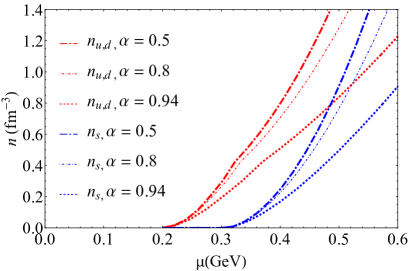
Figure 1: Quark number density ($n$) versus chemical potential ($\mu$). Notably, $n_{u,d}$ devotes to up and down quark number densities, and $n_{s}$ is related to the strange quark number density.

The following conditions should be imposed to obtain the EOS of SQM, which are:

$$\mu_{s}=\mu_{d}\equiv\mu,~{}~{}~{}\&~{}~{}~{}\mu_{u}=\mu-\mu_{e},$$

$$\frac{2}{3}n_{u}-\frac{1}{3}n_{d}-\frac{1}{3}n_{s}-n_{e}=0,$$

$$n_{B}=\dfrac{n_{u}+n_{d}+n_{s}}{3}.$$ (2)

The first two lines of Eq. (2) come from beta equilibrium and charge neutrality conditions, respectively. In the above conditions, $\mu_{i}$s $(i=u,d,s)$ are quark chemical potentials with flavor $i$, and $\mu_{e}$ is the electron chemical potential. $n_{i}$s $(i=u,d,s)$ are quark number densities with flavor $i$. In addition, $n_{B}$ is the baryon number density. Furthermore, $n_{e}=\mu_{e}^{3}/(3\pi^{2})$ is the electron number density. Then the pressure and the energy density can be obtained by the following relations

$$P=P_{0}+\int_{0}^{\mu_{j}}d\mu_{j}^{{}^{\prime}}\ n_{j}(\mu_{j}^{{}^{\prime}}),\ \ \ \ \ \ \ (j=u,d,s,e),$$

$$\epsilon=-P+\mu_{j}\ n_{j}(\mu_{j}),$$ (3)

where $P_{0}$ is the vacuum pressure, which is taken as the vacuum bag constant ($-B$). We consider two values for $B$ including $B^{1/4}=117MeV$ and $B^{1/4}=130MeV$. For these values of $B$, the energy per baryon of three-flavor quark matter is lower than that of two-flavor quark matter for $\alpha\leq 0.94$ ChengMingLi2020 . This condition is necessary for SQM to be the true ground state of the strong interaction weber 2005 . In the following, we present our results for the structural properties of SQS in massive gravity for different values of $B$ and $\alpha$. To this end, we first explain the modified TOV equation in massive gravity and then derive the differential equations to calculate the $\Lambda$ in this theory of gravity.

III Modified TOV Equation in Massive Gravity

Here, we consider dRGT-like massive gravity, which is introduced in Ref. Vegh . Notably, the dRGT-like massive gravity is similar to the dRGT massive theory of gravity, which is proposed by de Rham-Gabadadze-Tolley (dRGT) in 2011 deRham . The dRGT-like massive gravity’s action is given by Vegh

$$\mathcal{I}=\frac{1}{2\kappa^{2}}\int d^{4}x\sqrt{-g}\left[\mathcal{R}+m_{g}^{2}\sum_{i}^{4}c_{i}\mathcal{U}_{i}(g,f)\right]+\mathcal{I}_{matter},$$ (4)

where $\mathcal{R}$ and $m_{g}$ are the Ricci scalar and the graviton mass, respectively. It is notable that $\kappa^{2}=$ $8\pi$ because we consider $G=c=1$. Also, $f$ and $g$ are fixed symmetric and metric tensors, respectively. In the above action, $\mathcal{I}_{matter}$ is related to the action of matter. Moreover, $c_{i}$’s are free parameters of the massive theory, which are arbitrary constants. Notabley, their values can be determined according to theoretical or observational considerations Amico ; Akrami ; Berezhiani . $\mathcal{U}_{i}$’s are symmetric polynomials of the eigenvalues of $4\times 4$ matrix $K_{\nu}^{\mu}=\sqrt{g^{\mu\alpha}f_{\alpha\nu}}$ (where $g_{\mu\nu}$ is the dynamical (physical) metric, and $f_{\mu\nu}$ is the auxiliary reference metric, needed to define the mass term for gravitons) where they can be written in the following form

$$\mathcal{U}_{i}=\sum_{y=1}^{i}\left(-1\right)^{y+1}\frac{\left(i-1\right)!}{\left(i-y\right)!}\mathcal{U}_{i-y}\left[\mathcal{K}^{y}\right],$$ (5)

where $\mathcal{U}_{i-y}=1$, when $i=y$. Also, $\mathcal{K}$ stands for matrix square root, i.e., $\mathcal{K}_{~{}~{}~{}\nu}^{\mu}=\left(\sqrt{\mathcal{K}}\right)_{~{}~{}~{}\lambda}^{\mu}\left(\sqrt{\mathcal{K}}\right)_{~{}~{}~{}\upsilon}^{\lambda}$, and the rectangular bracket denotes the trace $\left[\mathcal{K}\right]=\mathcal{K}_{~{}~{}~{}\mu}^{\mu}$.

We consider the four-dimensional static spherical symmetric spacetime

$$ds^{2}=e^{2\Phi(r)}dt^{2}-\frac{dr^{2}}{e^{-2\lambda(r)}}-r^{2}h_{ij}dx_{i}dx_{j},~{}\text{where}~{}i,j=1,2.$$ (6)

where $e^{2\Phi(r)}$ and $e^{-2\lambda(r)}$ are unknown metric functions, and $h_{ij}dx_{i}dx_{j}=\left(d\theta^{2}+\sin^{2}\theta d\varphi^{2}\right)$. The equation of motion of dRGT-like massive gravity is given in the following form

$$G_{\mu}^{\nu}+m_{g}^{2}\chi_{\mu}^{\upsilon}=8\pi T_{\mu}^{\nu},$$ (7)

where $G_{\mu}^{\nu}$ is the Einstein tensor, and $T_{\mu}^{\nu}$ denotes the energy-momentum tensor which comes from the variation of $\mathcal{I}_{matter}$ and $\chi_{\mu\nu}$ is the massive term with the following explicit form

$$\chi_{\mu\nu}=-\sum_{i=1}^{d-2}\frac{c_{i}}{2}\left[\mathcal{U}_{i}g_{\mu\nu}+\sum_{y=1}^{i}\left(-1\right)^{y}\frac{\left(i!\right)\mathcal{U}_{i-y}\left[\mathcal{K}_{\mu\nu}^{y}\right]}{\left(i-y\right)!}\right].$$

Considering the quark stars as a perfect fluid, the nonzero components of the energy-momentum tensor are given by Behzad2017

$$T_{0}^{0}=\epsilon,~{}~{}~{}T_{1}^{1}=T_{2}^{2}=T_{3}^{3}=-P.$$ (8)

We follow the reference metric $f_{\mu\nu}$ for four-dimensional static spherical symmetric spacetime as it is considered for studying neutron stars and white dwarfs in the following form Behzad2017 ; Behzad2019

$$f_{\mu\nu}=diag(0,0,-J^{2},-J^{2}\sin^{2}\theta),$$ (9)

in which $J$ is known as a parameter of the reference metric, which is a positive constant. The explicit functional forms of $U_{i}$’s are given by Behzad2017

$$\mathcal{U}_{1} = \frac{2J}{r},$$

$$\mathcal{U}_{2} = \frac{2J^{2}}{r^{2}},$$

$$\mathcal{U}_{i} = 0,~{}~{}~{}~{}~{}i>2.$$ (10)

Using the field equation and reference and dynamical metrics, the metric function $e^{-2\lambda(r)}$, is obtained in the following form Behzad2017

$$e^{-2\lambda(r)}=1-m_{g}^{2}J\left(\frac{c_{1}r}{2}+c_{2}J\right)-\frac{2M(r)}{r},$$ (11)

in which $M(r)=\int_{0}^{R}4\pi r^{2}\epsilon(r)dr$ $\left(\text{or }\frac{dM(r)}{dr}=4\pi r^{2}\epsilon(r)\,\right)$. By definition $C_{1}\equiv m_{g}^{2}c_{1}J$ and $C_{2}\equiv m_{g}^{2}c_{2}J^{2}$ in Eq. (11), the modified TOV equation in massive gravity is given by Behzad2017

$$\frac{dP(r)}{dr}=\frac{\left(M(r)+4\pi r^{3}P-\frac{r^{2}C_{1}}{4}\right)\left(\epsilon+P\right)}{r\left(\frac{C_{1}r^{2}}{2}+2M(r)+r\left(C_{2}-1\right)\right)}.\,\,$$ (12)

Here, we obtain $\Lambda$ in massive gravity. To do this, we need to get a differential equation of metric function ($H(r)$) in massive gravity. In Appendix A, we have shown how we obtained this equation in massive gravity. Also, to check the correctness of the calculations, we have investigated the limit $C_{1}=C_{2}=0$ and shown that in this limit, the differential equation obtained in massive gravity is converted to the differential equation in GR. The differential equation to get $H(r)$ in massive gravity is

$$\left(A_{1}+A_{2}+A_{3}\right)H(r)+A_{4}\beta+\frac{d\beta}{dr}=0,$$ (13)

where $\beta=dH(r)/dr$, and $A_{i}$s are as follows

$$A_{1} = \frac{6}{r^{2}B_{1}},$$

$$A_{2} = \frac{B_{1}}{2r^{2}B_{1}^{2}}\left\{\frac{B_{2}\left(B_{2}f+B_{3}\right)}{B_{1}}-7B_{2}+3B_{3}\right.$$

$$+\frac{1}{B_{4}}\left[\frac{(f+1)B_{2}}{\left(B_{2}+\frac{C_{1}r}{2}\right)^{-1}}+\frac{2B_{1}\left(B_{2}+\frac{C_{1}r}{2}\right)}{B_{4}\left(\frac{2M\left(r\right)}{r}+8\pi r^{2}\epsilon-2\right)^{-1}}\right.$$

$$+16\pi r^{2}\left[\epsilon\left(\frac{C_{1}r}{4}+C_{2}+4\pi pr^{2}-1\right)\right.$$

$$\left.\left.\left.+\frac{3p}{\left(\frac{5C_{1}r}{12}+C_{2}+\frac{4\pi pr^{2}}{3}-1\right)^{-1}}+\frac{M\left(r\right)(7p+3\epsilon)}{r}\right]\right]\right\},$$

$$A_{3} = \frac{4\pi(p+\epsilon)f}{B_{1}},$$

$$A_{4} = \frac{2\left(\frac{3C_{1}r}{4}+2\pi r^{2}(\epsilon-p)+C_{2}-1\right)+\frac{2M\left(r\right)}{r}}{rB_{1}},$$ (14)

where $B_{1}$, $B_{2}$, $B_{3}$, and $B_{4}$ are

$$B_{1} = \frac{C_{1}r}{2}+C_{2}-1+\frac{2M\left(r\right)}{r},$$

$$B_{2} = 8\pi pr^{2}-\frac{C_{1}r}{2}+\frac{2M\left(r\right)}{r},$$

$$B_{3} = \frac{2M\left(r\right)}{r}-\frac{C_{1}r}{2}-8\pi\epsilon r^{2},$$

$$B_{4} = 1-\frac{2M\left(r\right)}{r},$$ (15)

also, $f$ is defined as $d\epsilon/dP$. In addition, $\Lambda$ is then obtained by

$$\Lambda=\frac{2}{3}k_{2}R^{5},$$ (16)

where $k_{2}$ is dimensionless tidal Love number for $l=2$, which is given as

$$k_{2} =\frac{16\sigma^{5}}{5}(1-2\sigma)^{2}\left[1+\sigma(y-1)-\frac{y}{2}\right]$$

$$\times\left\{12\sigma\left[1-\frac{y}{2}+\frac{\sigma(5y-8)}{2}\right]\right.$$

$$+4\sigma^{3}\left[13-11y+\sigma\left(3y-2\right)+2\sigma^{2}\left(1+y\right)\right]$$

$$+\left.6(1-2\sigma)^{2}\left[1+\sigma(y-1)-\frac{y}{2}\right]\ln\left(1-2\sigma\right)\right\}^{-1/2},$$ (17)

where $\sigma=M/R$ and $y$ is defined as $y=R\beta(R)/H(R)-4\pi R^{3}\epsilon_{0}/M$ in which $\epsilon_{0}$ is the energy density at the surface of the quark star ChengMingLi2020 . By simultaneously solving equations (12) and (13) along with $dM/dr=4\pi r^{2}\epsilon$, we obtain the curves of star mass in terms of radius and $\Lambda$ in terms of mass. The results are presented in the next section.

III.1 Modified Schwarzschild Radius

It is clear that by considering dRGT-like massive gravity, the Schwarzschild radius is modified. Using Eq. (11), we can get the Schwarzschild radius ($R_{Sch}$) for this theory of gravity. To find the modified Schwarzschild radius, we solve $S(r)=0$. So, the modified Schwarzschild radius for dRGT-like massive gravity is given Behzad2017

$$R_{Sch}=\frac{\left(1-C_{2}\right)}{C_{1}}-\frac{\sqrt{\left(C_{2}-1\right)^{2}-4C_{1}M}}{C_{1}},$$ (18)

where $M=M\left(r=R\right)$ is the star’s total mass (or the mass of the star on its surface).

III.2 Compactness

The compactness of a spherical object may be defined by the ratio of mass to radius of that object

$$\sigma=\frac{M}{R},$$ (19)

which may be indicated as the strength of gravity. In the following, we calculate the thermodynamic properties of SQM (EOS, speed of sound, and adiabatic index) for different values of $\alpha$ and $B$. We investigate the structural properties of SQS (mass, radius, dimensionless tidal deformability, compactness, and Schwarzschild radius) for a stiff EOS ($B^{1/4}=117MeV$), and a soft EOS ($B^{1/4}=130MeV$) in massive gravity. The value of $\Lambda$ depends not only on the EOS but also on the gravity used. In GR, the stiff EOSs cause the $\Lambda$ constraint to be lost and the soft EOSs can not cover the objects fall within in the mass gap region. We demonstrate that in massive gravity, the soft EOSs can not only lead to masses in the mass gap region but also satisfy the $\Lambda$ constraint well.

IV Equation of States of SQM for $B^{1/4}=117MeV$

In this section, we present our results for the thermodynamic properties of SQM in a modified NJL model for $B^{1/4}=117MeV$ and different values of $\alpha$. As it was mentioned in section II, by choosing this value of bag constant, the parameter $\alpha$ should be equal or less than $0.94$ to establish the stability condition of SQM. We derive the EOSs of SQM for different values of $\alpha$ including $\alpha=0.5$, $\alpha=0.8$, and $\alpha=0.94$. The results are presented in Fig. 2. This figure shows that the EOSs become stiffer by increasing the $\alpha$ parameter. We will show in section IV.1 that this behavior causes the mass of the star to increase. But it is possible that the structural features of these stars do not satisfy the constraints obtained from GW observations. Therefore, at the same time as the mass of the star increases, such constraints should also be checked. To check the causality, the speed of sound in terms of energy density is plotted in Fig. 3. The plots indicate that causality is established well for all $\alpha$ values. Also, with an increase in the value of $\alpha$, the speed of sound increases, which means that the EOS becomes stiffer and subsequently, the mass of the star becomes greater.

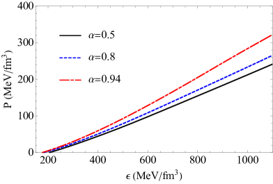
Figure 2: EOSs of SQM for $B^{1/4}=117MeV$ and different values of $\alpha$.

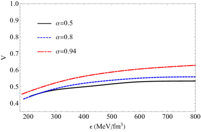
Figure 3: The speed of sound ($V$) energy density ($\epsilon$) for different values of $\alpha$.

As a measure of dynamical stability, the adiabatic index $\left(\Gamma=\frac{dP}{d\epsilon}\frac{P+\epsilon}{P}\right)$ has been presented as a function of energy density in Fig. 4. It is known that $\Gamma$ should be higher than $4/3$ for dynamical stability Behzad2017 ; Knutsen1988 ; Mak2013 ; Sedaghat20221 ; Hendi2016 . As one can see from this figure, this condition is satisfied for all values of $\alpha$.

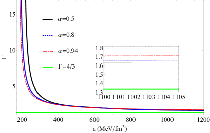
Figure 4: Adiabatic index ($\Gamma$) versus energy density ($\epsilon$) for $B^{1/4}=117MeV$ and different values of $\alpha$.

IV.1 Structural Properties of SQS in Massive Gravity for $B^{1/4}=117MeV$

In this section, we obtain the structural properties of SQS, including the $M-R$ and $\Lambda-M$ relations in dRGT-like massive gravity. We then compare the results with the constraints derived from astronomical observations. In addition, we obtain modified Schwarzschild radius and compactness of quark stars in this theory of gravity.

Practically, the modified TOV equation (12) is solved simultaneously with the equation, $M(r)=\int_{0}^{R}4\pi r^{2}\epsilon(r)dr$. To solve these equations, we have to consider the modified NJL EoS with the obtained pressure at the center of the star (i.e. $P(r=0)=P_{c}$, which $P_{c}$ is the central pressure of the quark star and given by the modified NJL EoS). Notably, the mass of the star at the center of the star is zero, i.e. $M(r=0)=0$. Then, we continue to solve the equations up to the star’s surface, where the pressure is zero ($P(r=R)=0$). The result is the mass and corresponding radius of the star (i.e. $M=M(R)$). We do this for different values of central pressures allowed by the mentioned EOS.

IV.1.1 $\alpha=0.5$

Now, we investigate the structural properties of SQS in massive gravity. We first use the obtained EOSs in section IV and the modified TOV equation (12) to derive the mass-radius ($M-R$) relation and $\Lambda-M$ relation in massive gravity. As we saw in section IV, we used three different values of $\alpha$ including $0.5$, $0.8$, and $0.94$ for the EOSs in the MNJL model. Now, we first examine the case $\alpha=0.5$. The equation (12) shows that there are two parameters, including $C_{1}$ and $C_{2}$, in massive gravity (these parameters are related to the dRGT-like massive gravity’s parameters). In the beginning, we set a fixed value for $C_{1}$ and investigate the structural features of SQS for different values of $C_{2}$. Figures 5 and 6 show the $M-R$ and $\Lambda-R$ diagrams, respectively, for $\alpha=0.5$, $C_{1}=10^{-5}$, and different values of $C_{2}$.

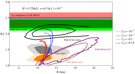
Figure 5: Mass-Radius diagram for $B^{1/4}=117MeV$, $\alpha=0.5,\hskip 2.84526ptC_{1}=10^{-5}$ and different values of $C_{2}$. The gray and orange regions are the mass - radius constraints from the GW170817 event. The black region shows pulsar J0740+6620, The green and black hatched regions represent pulsars J2215+5135 Linares2018 and PSR J095-0607, respectively. The red region amounts to the secondary component of GW190814. The brown and the purple regions show two different reports of the pulsar J0030+0451 Miller2019 ; Riley2019 .

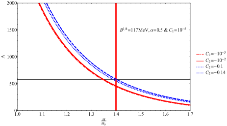
Figure 6: Dimensionless tidal deformability ($\Lambda$) versus mass of the star for $B^{1/4}=117MeV,\alpha=0.5,C_{1}=10^{-5}$ and different values of $C_{2}$. The horizontal black line and the vertical red line correspond to $\Lambda=580$ and $\frac{M}{{M}_{\odot}}=1.4$, respectively.

As one can see from Fig. 5, there are different colored regions in Fig. 5. The gray and orange areas are the $M-R$ constraints from GW170817. The black boundary corresponds to PSR J0740+6620 Cromartie2019 . The pink area represents the secondary component of GW190814 ZMiao2021 , and the green area shows the remnant mass of GW190425 JSedaghat . As one can see from this figure, we have not drawn graphs for the values $\arrowvert C_{2}\arrowvert>0.14$, because Fig. 6 shows for these values of $C_{2}$, the $\Lambda$ condition ($\Lambda_{1.4{M}_{\odot}}\lesssim 580$) is not satisfied. In Fig. 6, the horizontal black line shows the $\Lambda=580$, and the vertical red line represents $M=1.4{M}_{\odot}$. As one can see from this figure, the constraint $\Lambda_{1.4{M}_{\odot}}\lesssim 580$, is satisfied for $\lvert C_{2}\lvert\lesssim 0.14$ which corresponds to the $M_{TOV}\lesssim 2.13M_{\odot}$. Indeed, the maximum mass in this case cannot be more than $2.13M_{\odot}$. More details for structural properties of SQS for $B^{1/4}=117MeV$, $\alpha=0.5$, $C_{1}=10^{-5},$ and different values of $C_{2}$ are presented in Table. 1. Previously, in the Ref. ChengMingLi2020 the value of $M_{TOV}$ for $B^{1/4}=117MeV$ and $\alpha=0.5$ has been calculated in GR. The obvious difference between their result ($M_{TOV}=1.70M_{\odot}$) with the result obtained in this paper shows the important effect of the massive gravity in the mass of the SQS. Table. 1 demonstrates that by increasing the absolute value of $C_{2}$, the values of $M_{TOV}$, $\Lambda_{1.4{M}_{\odot}}$, and the compactness of the star are increased too. Additionally, The results calculated for $R_{Sch}$ show that the obtained masses can not be black holes.

Table 1: Structural properties of SQS for $B^{1/4}=117MeV,\alpha=0.5$, $C_{1}=10^{-5},$ and different values of $C_{2}$.

$C_{2}$	$-10^{-3}$	$-10^{-2}$	$-0.1$	$-0.14$
$R(km)$	$10.33$	$10.36$	$10.70$	$11.02$
$M_{TOV}({M}_{\odot})$	$1.76$	$1.78$	$2.02$	$2.13$
$\Lambda_{1.4{M}_{\odot}}$	$446.76$	$457.64$	$548.92$	$578.14$
$\sigma(10^{-1})$	$2.52$	$2.54$	$2.79$	$2.86$
$R_{Sch}(km)$	$5.20$	$5.22$	$5.43$	$5.53$

Now, we turn to the next case by choosing $B^{1/4}=117MeV$, $\alpha=0.5$, $C_{2}=-0.1$ and different values of $C_{1}$. It is shown in Refs. Hendi2016 ; Behzad2017 that changing the $C_{1}$ parameter has a negligible effect on the structural properties of the star. Therefore, in this section, we show this feature and for other values of $\alpha$ and the bag constant, we only change the value of $C_{2}$. Figure 7 represents the $M-R$ relation for different values of $C_{1}$.

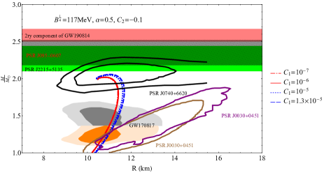
Figure 7: Mass-Radius diagram for $B^{1/4}=117MeV,\alpha=0.5$, $C_{2}=-0.1$, and different values of $C_{1}$. The gray and orange regions are the mass - radius constraints from the GW170817 event. The black region shows pulsar J0740+6620, The green and black hatched regions represent pulsars J2215+5135 Linares2018 and PSR J095-0607, respectively. The red region amounts to the secondary component of GW190814. The brown and the purple regions show two different reports of the pulsar J0030+0451 Miller2019 ; Riley2019 .

As this figure shows, changing the $C_{1}$ parameter has an insignificant effect on the maximum mass of the star. We have not plotted the results for values $C_{1}\gtrsim 1.3\times 10^{-5}$, because as the figure 8 shows, the condition $\Lambda_{1.4{M}_{\odot}}\lesssim 580$ is not established for these values of $C_{1}$. The structural properties of SQS for $B^{1/4}=117MeV$, $\alpha=0.5$, $C_{2}=-0.1$, and different values of $C_{1}$ are in Table. 2.

On the other hand, our results in Table. 2 indicate that the obtained objects cannot be black holes because the radii of these compact objects are bigger than the Schwarzschild radii. Besides, the strength of gravity increases by increasing the value of $\lvert C_{2}\lvert$.

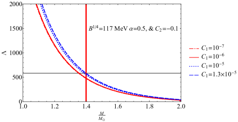
Figure 8: Dimensionless tidal deformability ($\Lambda$) versus mass of the star for $B^{1/4}=117MeV,\alpha=0.5$, $C_{2}=-0.1$, and different values of $C_{1}$. The horizontal black line and the vertical red line correspond to $\Lambda=580$ and $\frac{M}{{M}_{\odot}}=1.4$, respectively.

Table 2: Structural properties of SQS for $B^{1/4}=117MeV,\alpha=0.5$, $C_{2}=-0.1$, and different values of $C_{1}$.

$C_{1}$	$10^{-7}$	$10^{-6}$	$10^{-5}$	$1.3\times 10^{-5}$
$R(km)$	$10.61$	$10.92$	$10.95$	$10.99$
$M_{TOV}({M}_{\odot})$	$2.01$	$2.02$	$2.05$	$2.06$
$\Lambda_{1.4{M}_{\odot}}$	$473.77$	$480.89$	$548.92$	$578.25$
$\sigma(10^{-1})$	$2.80$	$2.74$	$2.77$	$2.77$
$R_{Sch}(km)$	$5.41$	$5.43$	$5.52$	$5.54$

IV.1.2 $\alpha=0.8$

Here, we increase the value of $\alpha$ and investigate its effect on the structure properties of the SQS in dRGT-like massive gravity. The figures. 9 and 10 show the $M-R$ and $\Lambda-M$ diagrams for $\alpha=0.8$,$\hskip 2.84526ptC_{1}=10^{-5}$, and different values of $C_{2}$, respectively.

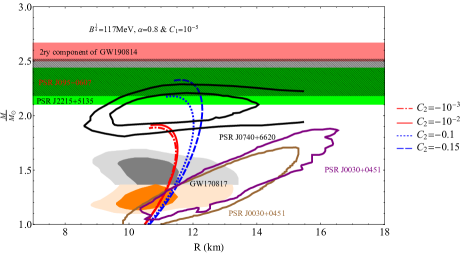
Figure 9: Mass-Radius diagram for $B^{1/4}=117MeV,\alpha=0.8,C_{1}=10^{-5}$, and different values of $C_{2}$. The gray and orange regions are the mass - radius constraints from the GW170817 event. The black region shows pulsar J0740+6620, The green and black hatched regions represent pulsars J2215+5135 Linares2018 and PSR J095-0607, respectively. The red region amounts to the secondary component of GW190814. The brown and the purple regions show two different reports of the pulsar J0030+0451 Miller2019 ; Riley2019 .

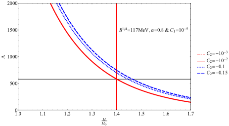
Figure 10: Dimensionless tidal deformability versus mass of the star for $B^{1/4}=117MeV,\alpha=0.8,\hskip 2.84526ptC_{1}=10^{-5},$ and different values of $C_{2}$. The horizontal black line and the vertical red line correspond to $\Lambda=580$ and $\frac{M}{{M}_{\odot}}=1.4$, respectively.

Comparison of figures 9 and 5 shows that the maximum mass of the star increases with the increase of $\alpha$ value. This result is obvious because we showed in Fig. 2 that the increase of $\alpha$ makes the EOS stiffer. However, Fig. 10 shows that this feature increases $\Lambda$ and the constraint $\Lambda_{1.4{M}_{\odot}}\lesssim 580$ is lost for $\arrowvert C_{2}\arrowvert\gtrsim 10^{-2}$ which corresponds to the $M_{TOV}\lesssim 2.33M_{\odot}$. Indeed, the maximum mass in this case cannot be more than $2.33M_{\odot}$. The structural properties of SQS for $B^{1/4}=117MeV$, $\alpha=0.8$, $C_{1}=10^{-5}$, and different values of $C_{2}$ are presented in Table. 3.

There are the same behaviors for the compactness and the modified Schwarzschild radius. They increase by increasing the value of $\lvert C_{2}\lvert$. Also, the radii of these compact objects are more than the modified Schwarzschild radii (i.e., $R>R_{Sch}$).

Table 3: Structural properties of SQS for $B^{1/4}=117MeV,\alpha=0.8$, $C_{1}=10^{-5}$, and different values of $C_{2}$.

$C_{2}$	$-10^{-3}$	$-10^{-2}$	$-0.1$	$-0.15$
$R(km)$	$10.80$	$10.92$	$11.33$	$11.61$
$M_{TOV}({M}_{\odot})$	$1.89$	$1.92$	$2.18$	$2.33$
$\Lambda_{1.4{M}_{\odot}}$	$578.35$	$578.69$	$700.07$	$745.67$
$\sigma(10^{-1})$	$2.59$	$2.60$	$2.85$	$2.97$
$R_{Sch}(km)$	$5.59$	$5.63$	$5.87$	$6.00$

IV.1.3 $\alpha=0.94$

For further investigation, we check the effect of massive gravity on the structural properties of SQS for $\alpha=0.94$. We do not consider values of $\alpha$ greater than $0.94$. Because, as mentioned in section II, the stability condition of SQM will be lost for $\alpha\gtrsim 0.94$ ChengMingLi2020 . BY setting $B^{1/4}=117MeV$, $\alpha=0.94$, $C_{1}=10^{-5}$, and different values of $C_{2}$, we obtain the Fig. 11, and 12 as the $M-R$ and $\Lambda-M$ diagrams, respectively. Here, we also see that with the increase of $\alpha$, the maximum gravitational mass increases, but as the EOS becomes stiffer, the $\Lambda$ constraint is no longer satisfied. Table. 4 shows the structural properties of SQS for $B^{1/4}=117MeV$, $\alpha=0.94$, $C_{1}=10^{-5}$, and different values of $C_{2}$. Although the values obtained for the $M_{TOV}$ for $\alpha=0.94$ are higher than those with $\alpha=0.5$ and $\alpha=0.8$, Table. 4 demonstrates that none of the results satisfy the constraint $\Lambda_{1.44M_{\odot}}\lesssim 580$.

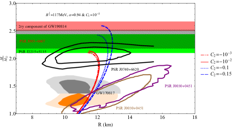
Figure 11: Mass-Radius diagram for $B^{1/4}=117MeV$, $\alpha=0.94$, $C_{1}=10^{-5}$, and different values of $C_{2}$. The gray and orange regions are the mass - radius constraints from the GW170817 event. The black region shows pulsar J0740+6620, The green and black hatched regions represent pulsars J2215+5135 Linares2018 and PSR J095-0607, respectively. The red region amounts to the secondary component of GW190814. The brown and the purple regions show two different reports of the pulsar J0030+0451 Miller2019 ; Riley2019 .

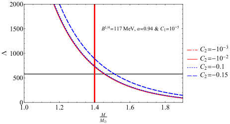
Figure 12: Dimensionless tidal deformability versus mass of the star for $B^{1/4}=117MeV$, $\alpha=0.94$, $C_{1}=10^{-5}$, and different values of $C_{2}$. The horizontal black line and the vertical red line correspond to $\Lambda=580$ and $\frac{M}{{M}_{\odot}}=1.4$, respectively.

Table 4: Structural properties of SQS for $B^{1/4}=117MeV,\alpha=0.94$, $C_{1}=10^{-5}$, and different values of $C_{2}$.

$C_{2}$	$-10^{-3}$	$-10^{-2}$	$-0.1$	$-0.15$
$R(km)$	$11.41$	$11.46$	$12.06$	$12.23$
$M_{TOV}({M}_{\odot})$	$2.11$	$2.13$	$2.43$	$2.60$
$\Lambda_{1.4{M}_{\odot}}$	$728.30$	$733.20$	$747.51$	$887.92$
$\sigma(10^{-1})$	$2.74$	$2.75$	$2.98$	$3.09$
$R_{Sch}(km)$	$6.24$	$6.30$	$6.54$	$6.70$

As an important result of our calculation, we could not describe the mass gap region and observational objects such as PSRJ0740+6620, the secondary component of GW190814, and the remnant mass of GW190425 by SQS when we considered the mentioned EOSs of SQM with $B^{1/4}=117MeV$ and different values of $\alpha$. In other words, the maximum mass of SQS with the mentioned EOSs in dRGT-like massive gravity is in the range $M_{TOV}<2.5M_{\odot}$.

To obtain massive SQSs that satisfy the $\Lambda$ constraint, we make the EOS soft. Because the value of $\Lambda$ depends on both the EOS and the gravity used, simultaneously. Therefore, in the next section, we change the value of the $B$ constant (as we expected) and investigate the results for thermodynamic properties of SQM and structural properties of SQS in dRGT-like massive gravity.

V Equation of States of SQM for $B^{1/4}=130MeV$

In the previous section, we saw that by increasing the value of $\alpha$, the EOS becomes stiffer, and subsequently the mass of the star increases, but the constraint $\Lambda_{1.44M_{\odot}}\lesssim 580$ is not satisfied for the SQSs fall within the mass gap region and consequently, a small range of the $C_{2}$ parameter is reachable. In this section, we increase the value of the bag constant, $B$, to make the EOS softer, and the condition of $\Lambda$ to be satisfied in a larger range of $C_{2}$ parameter. Figure 13 shows a comparison between two EOSs obtained from two different bag constants ($B^{1/4}=117MeV\$and$\ B^{1/4}=130MeV$). From this figure, it can be seen that the EOSs with the same value of $\alpha$ have the same slope and consequently have the same speed of sound. But the diagrams with $B^{1/4}=130MeV$ lie lower than those with $B^{1/4}=117MeV$. It shows that the EOSs with $B^{1/4}=130MeV$, are softer than those with $B^{1/4}=130MeV$. Although this result is obvious, we will indicate that it has a significant effect on the structural properties of SQS in massive gravity. This makes it possible to obtain quark stars that fall within the mass gap region and respect to the constraint $\Lambda_{1.4M_{\odot}}\lesssim 580$, simultaneously. Now, we set $B^{1/4}=130MeV$ and investigate its effect on the structural properties of SQS in massive gravity. In this situation, we consider another constraint too. We assume that the value of $\Lambda$ for $M_{TOV}$ should not be zero. Because otherwise the obtained mass is a black hole Chia2021 .

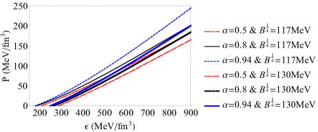
Figure 13: Comparison between EOSs for different values of $B$.

Figure. 14 represents the adiabatic index for different values of $\alpha$ and $B$. As this figure shows, for any choice of $\alpha$, dynamical stability is increased by increasing $B$.

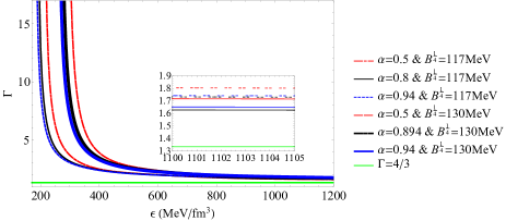
Figure 14: Adiabatic index ($\Gamma$) for different values $\alpha$ and $B$.

V.1 Structural Properties of SQS in Massive Gravity for $B^{1/4}=130MeV$

In the following, we study the structural properties of SQS in the presence of dRGT-like massive gravity for $B^{1/4}=130MeV$, and three different values of $\alpha=0.5$, $\alpha=0.8$, and $\alpha=0.94$.

V.1.1 $\alpha=0.5$

Here, we derive the structural properties of SQS in massive gravity for $\alpha=0.5$ and $B^{1/4}=130MeV$. Similar to the previous section, we first set a fixed value for $C_{1}$ and investigate $M-R$ and $\Lambda-M$ diagrams for different values of $C_{2}$. Figures 15 and 16 show $M-R$ and $\Lambda-M$ diagrams, respectively. We can see from the fig. 16 that all the diagrams satisfy the constraint $\Lambda_{1.4M_{\odot}}\lesssim 580$. The results show that by softening the EOS, the masses obtained in massive gravity not only satisfy the $\Lambda_{1.4{M}_{\odot}}\lesssim 580$ constraint, but also some of them are located in the mass gap region. As we can see from these figures, we did not use the values $\arrowvert C_{2}\arrowvert\gtrsim 0.84$, because they led to zero value for $\Lambda_{M_{TOV}}$. The results for structural properties are given in Table. 5.

As an important result, our findings indicate that the maximum mass of SQS can be in the range $M_{TOV}\lesssim 4M_{\odot}$. Indeed, by using the MNJL model with $B^{1/4}=130MeV$, and $\alpha=0.5$, SQSs fall within the mass gap region.

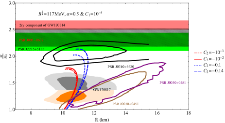
Figure 15: Mass-Radius diagram for $B^{1/4}=130MeV$, $\alpha=0.5$, $C_{1}=10^{-5}$, and different values of $C_{2}$. The gray and orange regions are the mass - radius constraints from the GW170817 event. The black region shows pulsar J0740+6620, The green and black hatched regions represent pulsars J2215+5135 Linares2018 and PSR J095-0607, respectively. The red region amounts to the secondary component of GW190814. The brown and the purple regions show two different reports of the pulsar J0030+0451 Miller2019 ; Riley2019 . The light blue band denotes the remnant mass of GW190425.

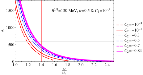
Figure 16: Dimensionless tidal deformability ($\Lambda$) versus mass of the star for $B^{1/4}=130MeV$, $\alpha=0.5$, $C_{1}=10^{-5}$, and different values of $C_{2}$. The horizontal black line and the vertical red line correspond to $\Lambda=580$ and $\frac{M}{{M}_{\odot}}=1.4$, respectively.

Table 5: Structural properties of SQS for $B^{1/4}=130MeV$, $\alpha=0.5$, $C_{1}=10^{-5}$, and different values of $C_{2}$. The results falling in mass gap have been separated in different column.

none mass gap					mass gap
$C_{2}$	$-10^{-3}$	$-0.1$	$-0.2$	$-0.3$	$-0.4$	$-0.5$	$-0.6$	$-0.7$	$-0.84$
$R(km)$	$9.04$	$9.46$	$9.85$	$10.24$	$10.66$	$11.06$	$11.40$	$11.75$	$12.34$
$M_{TOV}({M}_{\odot})$	$1.56$	$1.80$	$2.05$	$2.31$	$2.57$	$2.86$	$3.15$	$3.45$	$3.91$
$\Lambda_{1.4{M}_{\odot}}$	$185.80$	$255.06$	$307.00$	$348.34$	$379.38$	$403.35$	$431.03$	$449.16$	$480.18$
$\Lambda_{M_{TOV}}$	$59.11$	$26.20$	$12.74$	$6.20$	$3.30$	$1.42$	$0.64$	$0.26$	$0.02$
$\sigma(10^{-1})$	$2.55$	$2.82$	$3.08$	$3.34$	$3.57$	$3.83$	$4.09$	$4.34$	$4.69$
$R_{Sch}(km)$	$4.61$	$4.84$	$5.06$	$5.26$	$5.43$	$5.64$	$5.83$	$6.00$	$6.29$

V.1.2 $\alpha=0.8$

As a further investigation, we change the value of $\alpha$. Figures. 17, and 18 are $M-R$ and $\Lambda-M$ diagrams for $B^{1/4}=130MeV$, $\alpha=0.8$, $C_{1}=10^{-5}$ and different values of $C_{2}$, respectively. We can see that despite the increase of $\alpha$, which leads to the stiffer EOS, the constraint $\Lambda_{1.4{M}_{\odot}}\lesssim 580$ is still maintained. Here, the obtained masses lie in a larger area of the mass gap region compared to the previous case ($B^{1/4}=130MeV$ and $\alpha=0.5$). Moreover, we checked the $\Lambda$ of $M_{TOV}$ for different values of $C_{2}$. We observed that for $\arrowvert C_{2}\arrowvert\gtrsim 0.84$ the values of $\Lambda_{M_{TOV}}$ became zero. The results for structural properties are given in Table. 6.

On the other hand, our calculation for the compactness and the modified Schwarzschild radius show that these compact objects cannot be black holes because their radii are bigger than the Schwarzschild radii, i.e., $R>R_{Sch}$ (see Table. 6, for more details). Also, the compactness increases by increasing the value of $\lvert C_{2}\lvert$. In other words, the strength of gravity augments when the value of $\lvert C_{2}\lvert$ increases (see Table. 6, for more details).

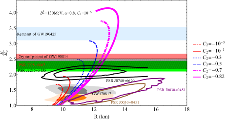
Figure 17: Mass-Radius diagram for $B^{1/4}=130MeV$, $\alpha=0.8$, $C_{1}=10^{-5}$, and different values of $C_{2}$. The gray and orange regions are the mass - radius constraints from the GW170817 event. The black region shows pulsar J0740+6620, The green and black hatched regions represent pulsars J2215+5135 Linares2018 and PSR J095-0607, respectively. The red region amounts to the secondary component of GW190814. The brown and the purple regions show two different reports of the pulsar J0030+0451 Miller2019 ; Riley2019 . The light blue band denotes the remnant mass of GW190425.

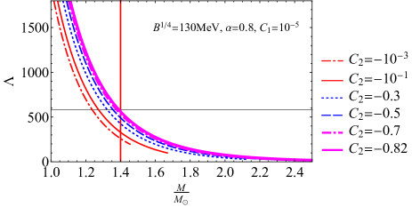
Figure 18: Dimensionless tidal deformability ($\Lambda$) versus mass of the star for $B^{1/4}=130MeV$, $\alpha=0.8$, $C_{1}=10^{-5}$, and different values of $C_{2}$. The horizontal black line and the vertical red line correspond to $\Lambda=580$ and $\frac{M}{{M}_{\odot}}=1.4$, respectively.

Table 6: Structural properties of SQS for $B^{1/4}=130MeV$, $\alpha=0.8$, $C_{1}=10^{-5}$, and different values of $C_{2}$. The results falling in mass gap have been separated in different column.

none mass gap				mass gap
$C_{2}$	$-10^{-3}$	$-0.1$	$-0.2$	$-0.3$	$-0.4$	$-0.5$	$-0.6$	$-0.7$	$-0.82$
$R(km)$	$9.46$	$9.94$	$10.40$	$10.78$	$11.15$	$11.60$	$11.97$	$12.36$	$12.80$
$M_{TOV}({M}_{\odot})$	$1.68$	$1.94$	$2.21$	$2.49$	$2.79$	$3.09$	$3.40$	$3.73$	$4.14$
$\Lambda_{1.4{M}_{\odot}}$	$257.98$	$329.76$	$383.76$	$427.33$	$461.80$	$487.14$	$515.31$	$536.06$	$559.21$
$\Lambda_{M_{TOV}}$	$47.04$	$20.43$	$9.64$	$2.70$	$1.95$	$0.92$	$0.39$	$0.14$	$0.01$
$\sigma(10^{-1})$	$2.63$	$2.89$	$3.14$	$3.42$	$3.70$	$3.94$	$4.20$	$4.47$	$4.79$
$R_{Sch}(km)$	$4.97$	$5.22$	$5.45$	$5.67$	$5.90$	$6.10$	$6.29$	$6.49$	$6.73$

It is notable that by considering the MNJL model with $B^{1/4}=130MeV$, and $\alpha=0.8$, the maximum mass of SQSs can be in the range $1.68M_{\odot}\lesssim M_{TOV}\lesssim 4.2M_{\odot}$, which fall within the mass gap region.

V.1.3 $\alpha=0.94$

As the final investigation of SQS in dRGT-like massive gravity, we consider $B^{1/4}=130MeV$ and $\alpha=0.94$. Figures. 19, and 20 show $M-R$ and $\Lambda-M$ diagrams for $C_{1}=10^{-5}$ and different values of $C_{2}$, respectively. Figure 20 shows that for values $\arrowvert C_{2}\arrowvert\gtrsim 0.54$, the constraint $\Lambda_{1.4{M}_{\odot}}\lesssim 580$ is no longer satisfied. For this reason, compared to the case $\alpha=0.8$, a smaller area of the $C_{2}$ parameter is accessible, which results from the sharpness of the EOS. The structural properties of SQS for $B^{1/4}=130MeV$, $\alpha=0.94$, $C_{1}=10^{-5}$ and different values of $C_{2}$ are presented in Table. 7.

Briefly, the maximum mass of SQSs with $B^{1/4}=130MeV$, and $\alpha=0.94$, cannot be more than $3.45{M}_{\odot}$. However, the mentioned values of the parameters of our system can satisfy the mass gap region (see Table. 7, for more details). Besides, there are the same behaviors of the compactness and the Schwarzschild radius when the value of $\lvert C_{2}\lvert$ increases. In other words, the strength of gravity augments by increasing the value of $\lvert C_{2}\lvert$.

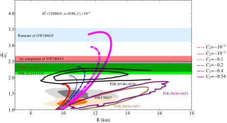
Figure 19: Mass-Radius diagram for $B^{1/4}=130MeV$, $\alpha=0.94$, $C_{1}=10^{-5}$, and different values of $C_{2}$. The gray and orange regions are the mass - radius constraints from the GW170817 event. The black region shows pulsar J0740+6620, The green and black hatched regions represent pulsars J2215+5135 Linares2018 and PSR J095-0607, respectively. The red region amounts to the secondary component of GW190814. The brown and the purple regions show two different reports of the pulsar J0030+0451 Miller2019 ; Riley2019 . The light blue band denotes the remnant mass of GW190425.

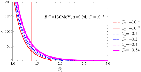
Figure 20: Dimensionless tidal deformability versus mass of the star for $B^{1/4}=130MeV$, $\alpha=0.94$, $C_{1}=10^{-5}$, and different values of $C_{2}$. The horizontal black line and the vertical red line correspond to $\Lambda=580$ and $\frac{M}{{M}_{\odot}}=1.4$, respectively.

Table 7: Structural properties of SQS for $B^{1/4}=130MeV$, $\alpha=0.94$, $C_{1}=10^{-5}$, and different values of $C_{2}$. The results falling in mass gap region have been separated in a different column.

none mass gap					mass gap
$C_{2}$	$-10^{-3}$	$-10^{-2}$	$-0.1$	$-0.2$	$-0.3$	$-0.4$	$-0.54$	$-0.55$
$R(km)$	$9.81$	$9.85$	$10.30$	$10.77$	$11.23$	$11.63$	$12.32$	$12.35$
$M_{TOV}({M}_{\odot})$	$1.79$	$1.81$	$2.06$	$2.35$	$2.65$	$2.96$	$3.42$	$3.45$
$\Lambda_{1.4{M}_{\odot}}$	$326.43$	$333.26$	$398.93$	$452.51$	$499.87$	$532.37$	$578.95$	$580.64$
$\Lambda_{M_{TOV}}$	$32.25$	$32.26$	$15.20$	$6.51$	$2.92$	$1.36$	$0.35$	$0.32$
$\sigma$ $(10^{-1})$	$2.70$	$2.72$	$2.96$	$3.23$	$3.49$	$3.77$	$4.11$	$4.13$
$R_{Sch}(km)$	$5.29$	$5.30$	$5.54$	$5.80$	$6.03$	$6.26$	$6.57$	$6.59$

As a final point, by considering the MNJL model with $B^{1/4}=130MeV$ and different values of $\alpha$ ($0.5<\alpha<0.94$), we indicated that the mass of SQSs could be in the mass gap region. So, it seems reasonable to consider SQSs in massive gravity as candidates for the mass gap region.

VI Conclusion

We investigated the structural properties of quark star in massive gravity. In this study, we considered three-flavor quark matter (up, down and strange flavors) in MNJL model ChengMingLi2020 which is a combination of NJL Lagrangian and its Fierz transformation by using weighting factors ($1-\alpha$) and $\alpha$. By imposing charge neutrality and chemical equilibrium, we obtained the EOSs of SQM for three different values of $\alpha$, ($\alpha=0.5$, $\alpha=0.8$, and $\alpha=0.94$) and two different values of Bag constant ($B^{1/4}=117MeV$ and $B^{1/4}=130MeV$). We ensured that the EOSs satisfied causality and dynamical stability conditions. We then presented a brief introduction on the modified TOV equation in massive gravity. We explained the parameters appeared in TOV equation in massive gravity, including $C_{1}$ and $C_{2}$. We also derived the differential equation for the metric function $H(r)$ in massive gravity to calculate the tidal deformability.

To assess the structural properties of SQS, we initially considered $B^{1/4}=117MeV$ in the EOS and then by setting a fixed value for $C_{1}$ (the mass-radius relation is independent of $C_{1}$ Behzad2017 ) and selecting different values of $C_{2}$, we calculated the structural properties of SQS. The results analyzed to ensure compliance with the constraint $\Lambda_{1.4{M}_{\odot}}\lesssim 580$. We observed that increasing the $\alpha$ parameter led to an increase in the maximum gravitational mass but also resulted the aforementioned constraint to be satisfied in a smaller range of massive gravity parameters. Consequently, the allowed mass range of the star decreased. For the case of $B^{1/4}=117MeV$, we obtained the maximum allowed $M_{TOV}$ approximately $2.13M_{\odot}$.

Subsequently, we altered, the value of $B$ and considered $B^{1/4}=130MeV$. This change resulted in a softer EOS and a broader range of massive parameters satisfying the astronomical constraints. We obtained masses that fall within the mass gap region ($M\sim(2.5-5)M_{\odot}$) that simultaneously satisfied all the observational constraints. Moreover, we calculated Schwarzschild radius to show that compact objects studied in this paper were not black holes.

In general relativity, soft EOSs yield small masses for quark stars, while stiff EOSs fail to satisfy the the $\Lambda$ constraint. However, our study showed that massive gravity allows for the existence of quark stars with higher masses than those predicted by general relativity, while still satisfying the constraints imposed by gravitational wave observations.

Finally in Appendix B, by considering a constant value of $\alpha$ ($\alpha=0.8$), we increased the value of the bag constant to show that our results in massive gravity still cover the mass gap region.

Appendix A

To calculate the tidal deformability, we need to obtain the metric function $H(r)$, which satisfies the following equation

$$\left(-\frac{6e^{2\lambda}}{r^{2}}-2(\Phi^{\prime})^{2}+2\Phi^{\prime\prime}+\frac{3}{r}\lambda^{\prime}\right.$$

$$\left.+\frac{7}{r}\Phi^{\prime}-2\Phi^{\prime}\lambda^{\prime}+\frac{f}{r}(\Phi^{\prime}+\lambda^{\prime})\right)H$$

$$+\left(\frac{2}{r}+\Phi^{\prime}-\lambda^{\prime}\right)\beta+\frac{d\beta}{dr}=0,$$ (20)

Here $\beta=dH/dr$, $f$ corresponds to $d\epsilon/dp$. Also, $\Phi^{\prime}$ satisfies the following equation

$$\Phi^{\prime}=-\frac{p^{\prime}}{(\epsilon+p)},$$ (21)

where $p^{\prime}$ satisfies TOV equation in massive gravity.

$$p^{\prime}=\frac{(p+\epsilon)B_{2}}{2rB_{1}},$$ (22)

$$M^{\prime}\left(r\right)=4\pi r^{2}\epsilon,$$ (23)

where $B_{1}=$ $\frac{C_{1}r}{2}+C_{2}-1+\frac{2M\left(r\right)}{r}$, and $B_{2}=8\pi pr^{2}-\frac{C_{1}r}{2}+\frac{2M\left(r\right)}{r}$.

By deriving relations (21) and (22) with respect to $r$ we get

$$\Phi^{\prime\prime}=\frac{\left(1+f\right){p^{\prime}}^{2}-p^{\prime\prime}(\epsilon+p)}{(\epsilon+p)^{2}},$$ (24)

and

$$p^{\prime\prime} =\frac{\left(1+f\right)B_{2}p^{\prime}}{2rB_{1}}$$

$$+\frac{\left(4\pi r^{2}\left(rp^{\prime}+\epsilon\right)+8\pi r^{2}p-\frac{C_{1}r}{4}-\frac{M}{r}\right)(p+\epsilon)}{r^{2}B_{1}}$$

$$-\frac{\left(C_{1}r+C_{2}-1+8\pi r^{2}\epsilon\right)(p+\epsilon)B_{2}}{2r^{2}B_{1}^{2}}.$$ (25)

In Eq. (20), $\lambda^{\prime}$ satisfies the following equation

$$\lambda^{\prime}=\frac{s^{\prime}}{2s},$$ (26)

where

$$s=\frac{-1}{B_{1}},$$ (27)

and

$$s^{\prime}=\frac{\frac{C_{1}}{2}+\frac{2M^{\prime}\left(r\right)}{r}-\frac{2M\left(r\right)}{r^{2}}}{B_{1}^{2}}.$$ (28)

Now, for the convenience of calculations, we write equation (20) as below

$$\left(A_{1}+A_{2}+A_{3}\right)H+A_{4}\beta+\frac{d\beta}{dr}=0,$$ (29)

where $A_{1}$, $A_{2}$, $A_{3}$, and $A_{4}$ are defined as follows.

$$A_{1}\equiv-\frac{6e^{2\lambda}}{r^{2}},$$ (30)

$$A_{2}\equiv-2\left(\Phi^{\prime}\right)^{2}+2\Phi^{\prime\prime}+\frac{3\lambda^{\prime}}{r}+\frac{7\Phi^{\prime}}{r}-2\lambda^{\prime}\Phi^{\prime},$$ (31)

$$A_{3}\equiv\frac{(\Phi^{\prime}+\lambda^{\prime})f}{r},$$ (32)

and

$$A_{4}\equiv\frac{2}{r}+\Phi^{\prime}-\lambda^{\prime}.$$ (33)

Now using Eqs. (21) to (28), we obtain the following terms for coefficients $A_{1}$ to $A_{4}$.

$$A_{1}=\frac{6}{r^{2}B_{1}},$$ (34)

$$A_{2} =\frac{B_{1}}{2r^{2}B_{1}^{2}}\left\{\frac{B_{2}\left(B_{2}f+B_{3}\right)}{B_{1}}-7B_{2}+3B_{3}\right.$$

$$+\frac{1}{B_{4}}\left[\frac{(f+1)B_{2}}{\left(B_{2}+\frac{C_{1}r}{2}\right)^{-1}}+\frac{2B_{1}\left(B_{2}+\frac{C_{1}r}{2}\right)}{B_{4}\left(\frac{2M\left(r\right)}{r}+8\pi r^{2}\epsilon-2\right)^{-1}}\right.$$

$$+16\pi r^{2}\left[\epsilon\left(\frac{C_{1}r}{4}+C_{2}+4\pi pr^{2}-1\right)\right.$$

$$\left.\left.\left.+\frac{3p}{\left(\frac{5C_{1}r}{12}+C_{2}+\frac{4\pi pr^{2}}{3}-1\right)^{-1}}+\frac{M\left(r\right)(7p+3\epsilon)}{r}\right]\right]\right\},$$ (35)

$$A_{3}=\frac{4\pi(p+\epsilon)f}{B_{1}},$$ (36)

$$A_{4}=\frac{2\left(\frac{3C_{1}r}{4}+2\pi r^{2}(\epsilon-p)+C_{2}-1\right)+\frac{2M\left(r\right)}{r}}{rB_{1}}.$$ (37)

where $B_{3}=\frac{2M\left(r\right)}{r}-\frac{C_{1}r}{2}-8\pi\epsilon r^{2}$, and $B_{4}=1-\frac{2M\left(r\right)}{r}$.

To check the correctness of the calculations, we consider the case $C_{1}=C_{2}=0$ and show that Eq. (29) converts to the equation obtained in Einstein’s gravity

$$\frac{20H}{B_{4}}\left(\pi\left(\epsilon+\frac{9p+(\epsilon+p)f}{10}\right)-\frac{3}{10r^{2}}-\frac{\left(B_{2}+\frac{C_{1}r}{2}\right)^{2}}{20rB_{4}}\right)$$

$$-\frac{\left(\frac{2M\left(r\right)}{r}+4\pi r^{2}(\epsilon-p)-2\right)H}{r\left(1-\frac{2M\left(r\right)}{r}\right)}^{\prime}+H^{\prime\prime}=0.$$ (38)

By considering $C_{1}=C_{2}=0$, Eqs. (34) to (36) are converted to

$$A_{1}=\frac{-6}{r^{2}B_{4}},$$ (39)

$$A_{2}=\frac{4\pi B_{4}(9p+5\epsilon)-\left(B_{2}+\frac{C_{1}r}{2}\right)^{2}}{B_{4}^{2}},$$ (40)

$$A_{3}=\frac{4\pi(p+\epsilon)f}{B_{4}}.$$ (41)

It is clear that the sum of Eqs. (39) to (41) gives the coefficient of $H$ in equation (38). Furthermore, by considering $C_{1}=C_{2}=0$, Eq. (36) becomes

$$A_{4}=\frac{2\left(1+2\pi r^{2}(p-\epsilon)-\frac{M\left(r\right)}{r}\right)}{rB_{4}},$$ (42)

which is equivalent to the coefficient of function $H^{\prime}$ in equation (38).

Appendix B

In the previous sections, we have considered two different values for the bag constant, namely $B^{1/4}=117MeV$ and $B^{1/4}=130MeV$ (similar to Ref. ChengMingLi2020 ). The reason for choosing these two values of $B$ is to compare the structural properties of the SQS in massive gravity (which we have done in this paper) with the results obtained in Einstein gravity with the same values of $B$ (which was done in Ref. ChengMingLi2020 ). One question that might arise is the effect of increasing the bag constant on the structural properties of SQS. In this appendix, we increase $B$ and check whether the results cover the mass gap region. The determination of the range of $B$ depends on various factors, such as the model used to obtain the EOS, the number of quark flavors, the mass of the quarks, etc. If we take into account the constraint of tidal deformability, determination of the range of $B$ also depends on the gravity used. This is because to obtain $\Lambda$, not only the EOS (in which $B$ appears) is effective, but also the gravity used is important. For example in Ref. Stergioulas , by using MIT bag model and considering $m_{s}=0$ ($m_{s}$ is the mass of strange quark), $B$ is constrained in the range $58.9\frac{MeV}{fm^{3}}<B<91.5\frac{MeV}{fm^{3}}$. In Farhi1984 by assuming $m_{s}=150MeV$, the range of $B$ is $56-78\frac{MeV}{fm^{3}}$. In Aziz2019 by studying 20 compact stars, $B$ is obtained in the range $41.58-319.31\frac{MeV}{fm^{3}}$. In Ref. Zhou2018 , using perturbative QCD and the $\Lambda$ constraint from GW170817, $B^{\frac{1}{4}}$ is constrained to a narrow range from 134.1$MeV$ to 141.4 $MeV$ ($42\frac{MeV}{fm^{3}}<B<52\frac{MeV}{fm^{3}}$). In Song1992 $B$ is in the range $100-200MeV^{4}$ ($13\frac{MeV}{fm^{3}}<B<208\frac{MeV}{fm^{3}}$). In this paper, we increase the value of $B$ in the MNJL model for a fixed value of $\alpha$ (e.g. $\alpha=0.8$) and investigate its effect on the structural properties of SQS in massive gravity. In the following, we choose two different values for $B$ including $B^{\frac{1}{4}}=140MeV$ ($B=50\frac{MeV}{fm^{3}}$) and $B^{\frac{1}{4}}=148MeV$ ($B=62\frac{MeV}{fm^{3}}$) and check whether the results cover the mass gap region. We show that for these values of $B$, the results fall within the mass gap region. We do not try the values $\alpha=0.8$, and $B^{\frac{1}{4}}>148MeV$, because for these values, the results do not satisfy the constraint $70\lesssim\Lambda_{1.4{M}_{\odot}}\lesssim 580$.

B.1 The results for $\alpha=0.8$ and $B^{\frac{1}{4}}=140MeV$

Now we increase the value of $B^{\frac{1}{4}}$ to $140MeV$ and show that the results are still in the mass gap region. We first investigate the stability condition of SQM. Figure. 21 shows that the energy per baryon of three-flavor quark matter is less than that of two-flavor quark matter for $B^{1/4}=140MeV$ and $\alpha=0.8$ in all baryon number densities. In the following, we investigate $\Lambda-M$ and $M-R$ diagrams for $B^{1/4}=140MeV$, $\alpha=0.8$, $C_{1}=10^{-5}$, and different values of $C_{2}$ parameter. Figure. 22 shows that the condition $70\lesssim\Lambda_{1.4{M}_{\odot}}\lesssim 580$ is fulfilled for all values of $C_{2}$. Compared to the Fig. 18 ($\alpha=0.8$ and $B^{1/4}=130MeV$), we can see that the values of $\Lambda$ decrease with the increase of $B$. This result is obvious, because as $B$ increases, the EOS becomes softer and consequently $\Lambda$ decreases.

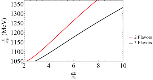
Figure 21: Energy per baryon versus baryon number density for $B^{1/4}=140MeV$ and $\alpha=0.8$. $n_{0}$ is the nuclear saturation density which is equal to $0.16fm^{-3}$.

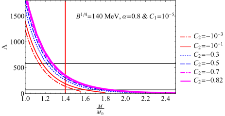
Figure 22: Dimensionless tidal deformability ($\Lambda$) versus mass of the star for $B^{1/4}=140MeV$, $\alpha=0.8$, $C_{1}=10^{-5}$, and different values of $C_{2}$. The upper black line, the lower black line, and the vertical red line correspond to $\Lambda=580$, $\Lambda=70$, and $\frac{M}{{M}_{\odot}}=1.4$, respectively.

Figure. 23 represents $M-R$ diagram for $B^{1/4}=140MeV$, $\alpha=0.8$, $C_{1}=10^{-5}$, and different values of $C_{2}$. We can see that the results still cover the mass gap region. However, compared to the Fig. 17 ($\alpha=0.8$ and $B^{1/4}=130MeV$), the results are obtained in a narrower range of the mass gap. In fact, such a result can be expected by making the EOS softer.

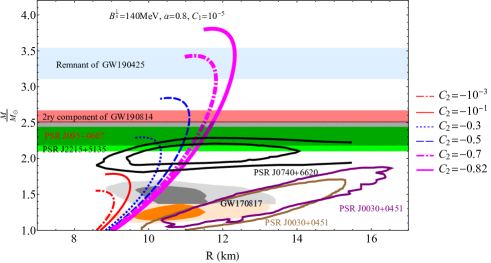
Figure 23: Mass-Radius diagram for $B^{1/4}=140MeV$, $\alpha=0.8$, $C_{1}=10^{-5}$, and different values of $C_{2}$. The gray and orange regions are the mass - radius constraints from the GW170817 event. The black region shows pulsar J0740+6620, The green and black hatched regions represent pulsars J2215+5135 Linares2018 and PSR J095-0607, respectively. The red region amounts to the secondary component of GW190814. The brown and the purple regions show two different reports of the pulsar J0030+0451 Miller2019 ; Riley2019 . The light blue band denotes the remnant mass of GW190425.

B.2 The results for $\alpha=0.8$ and $B^{\frac{1}{4}}=148MeV$

For further investigation, we increase the value of $B^{1/4}$ to $148MeV$. First of all, we have to check the stability condition of the SQM. Figure. 24 shows that this condition is well established for all baryon number densities.

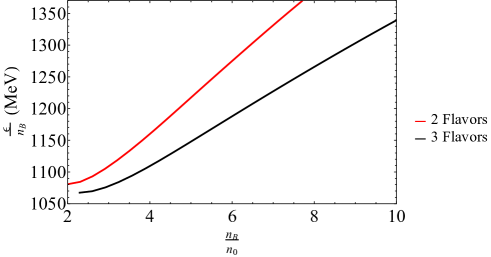
Figure 24: Energy per baryon versus baryon number density for $B^{1/4}=148MeV$ and $\alpha=0.8$. $n_{0}$ is the nuclear saturation density which is equal to $0.16fm^{-3}$.

In the next step, we examine the $\Lambda$ behavior. Figure. 25 represents $\Lambda-M$ diagram for $B^{1/4}=148MeV$, $\alpha=0.8$, $C_{1}=10^{-5}$, and different values of $C_{2}$. As we can see from this figure, the results respect to the constraint $70\lesssim\Lambda_{1.4{M}_{\odot}}\lesssim 580$. It is worth noting that for $\alpha=0.8$ and $B^{\frac{1}{4}}>148MeV$ the EOS becomes so soft that the $\Lambda_{1.4{M}_{\odot}}$ is below $70$ for some values of $C_{2}$ and the constraint $70\lesssim\Lambda_{1.4{M}_{\odot}}\lesssim 580$ is lost. Therefore, we consider $B^{1/4}=148MeV(B=62\frac{MeV}{fm^{3}})$ as the maximum allowable value of the bag constant in the MNJL model for $\alpha=0.8$ to study the structural properties of SQM in massive gravity.

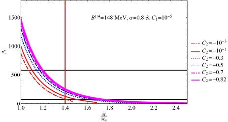
Figure 25: Dimensionless tidal deformability ($\Lambda$) versus mass of the star for $B^{1/4}=148MeV$, $\alpha=0.8$, $C_{1}=10^{-5}$, and different values of $C_{2}$. The upper black line, the lower black line, and the vertical red line correspond to $\Lambda=580$, $\Lambda=70$, and $\frac{M}{{M}_{\odot}}=1.4$, respectively.

Figure. 26 shows $M-R$ diagram for $B^{1/4}=148MeV$, $\alpha=0.8$, $C_{1}=10^{-5}$, and different values of $C_{2}$. As this figure shows, despite increasing $B$, the results still fall within the mass gap region. As mentioned above, this value of $B$ is the maximum possible value to meet $\Lambda_{1.4{M}_{\odot}}$ constraint in MNJL for $\alpha=0.8$ in massive gravity.

Figure 26: Mass-Radius diagram for $B^{1/4}=148MeV$, $\alpha=0.8$, $C_{1}=10^{-5}$, and different values of $C_{2}$. The gray and orange regions are the mass - radius constraints from the GW170817 event. The black region shows pulsar J0740+6620, The green and black hatched regions represent pulsars J2215+5135 Linares2018 and PSR J095-0607, respectively. The red region amounts to the secondary component of GW190814. The brown and the purple regions show two different reports of the pulsar J0030+0451 Miller2019 ; Riley2019 . The light blue band denotes the remnant mass of GW190425.