Partial Search in a Frozen Network is Enough to Find a Strong Lottery Ticket

Abstract

Randomly initialized dense networks contain subnetworks that achieve high accuracy without weight learning—strong lottery tickets (SLTs). Recently, Gadhikar et al. (2023) demonstrated theoretically and experimentally that SLTs can also be found within a randomly pruned source network, thus reducing the SLT search space. However, this limits the search to SLTs that are even sparser than the source, leading to worse accuracy due to unintentionally high sparsity. This paper proposes a method that reduces the SLT search space by an arbitrary ratio that is independent of the desired SLT sparsity. A random subset of the initial weights is excluded from the search space by freezing it—i.e., by either permanently pruning them or locking them as a fixed part of the SLT. Indeed, the SLT existence in such a reduced search space is theoretically guaranteed by our subset-sum approximation with randomly frozen variables. In addition to reducing search space, the random freezing pattern can also be exploited to reduce model size in inference. Furthermore, experimental results show that the proposed method finds SLTs with better accuracy and model size trade-off than the SLTs obtained from dense or randomly pruned source networks. In particular, the SLT found in a frozen graph neural network achieves higher accuracy than its weight trained counterpart while reducing model size by $40.3\times$.

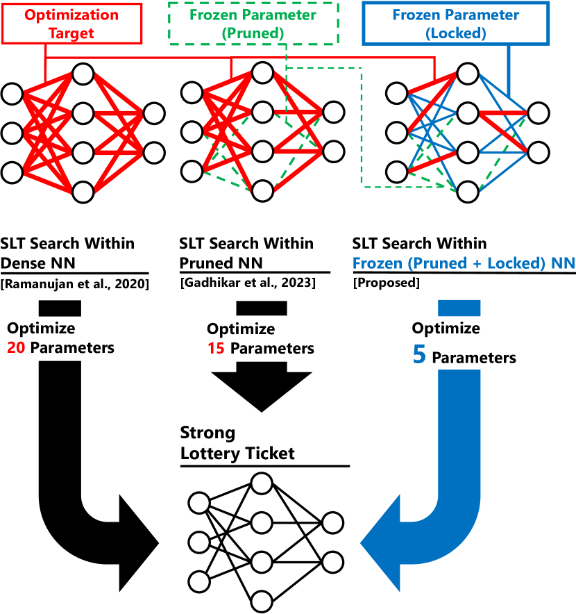
Figure 1: Freezing the source network by randomly pruning some parameters and locking others reduces the optimization targets for finding an SLT.

1 Introduction

The Strong Lottery Ticket Hypothesis (SLTH) conjectured the existence of subnetworks within a randomly weighted network—strong lottery tickets (SLTs)—that achieve comparable accuracy to trained dense networks (Zhou et al., 2019; Ramanujan et al., 2020; Malach et al., 2020). The existence of such subnetworks that do not require weight learning, illustrated in Figure 1(left), has been demonstrated experimentally (Zhou et al., 2019; Ramanujan et al., 2020; Huang et al., 2022; López García-Arias et al., 2023; Yeo et al., 2023) and proven theoretically for dense source networks (Malach et al., 2020; Orseau et al., 2020; Pensia et al., 2020; Diffenderfer & Kailkhura, 2021; da Cunha et al., 2021; Burkholz, 2022a; Burkholz et al., 2022; Ferbach et al., 2023; Gadhikar et al., 2023).

Since SLTs can be reconstructed from the random seed of the weights and a supermask (a simple binary pruning mask), potentially eliminating the need for storing and loading weights from memory, they offer a particularly advantageous opportunity for specialized inference hardware (Hirose et al., 2022). However, the existing algorithms for finding SLTs suffer from the same high computational cost as weight optimization, since they also employ backpropagation to update one parameter per neural connection (Ramanujan et al., 2020; Zhou et al., 2021; Diffenderfer & Kailkhura, 2021; Sreenivasan et al., 2022).

Recently, Gadhikar et al. (2023) demonstrated that this steep training cost can be alleviated by randomly pruning the source network at initialization, reducing the number of edges to be optimized (see Figure 1, center). However, this limits the SLT search space to the high sparsity region, which may not offer the optimal accuracy.

This paper introduces a novel method that reduces the search space by an arbitrary ratio independent of the desired SLT sparsity: in addition to random pruning at initialization, it also locks randomly chosen parameters at initialization to be a permanent part of the SLT (i.e., never pruned), as exemplified in Figure 1(right). Both the pruned and the locked parameters—the frozen parameters—are excluded from the search space, therefore reducing the training cost. Excluding them from the supermask also reduces the model size in inference, as the random freezing pattern can also be regenerated from its seed (Wimmer et al., 2020).

Moreover, our experiments show that SLTs found within frozen networks can achieve a better accuracy to model size trade-off than SLTs obtained from dense (Ramanujan et al., 2020; Sreenivasan et al., 2022) or sparse (Gadhikar et al., 2023) random networks. In addition to demonstrating this method experimentally, this paper also provides a mathematical analysis of the existence of SLTs within such partially frozen source networks.

In summary, this paper proposes a novel method that features the following contributions:

• It reduces the SLT search space regardless of the desired SLT sparsity by random partial freezing (pruning and locking) of the source random network.

• The proposed method is theoretically supported by our SLT existence result based on subset-sum approximation with randomly frozen variables.

• Experimental results show that SLTs found in the frozen network achieve better accuracy-to-search space and accuracy-to-model size trade-offs than SLTs found within dense or sparse random networks.

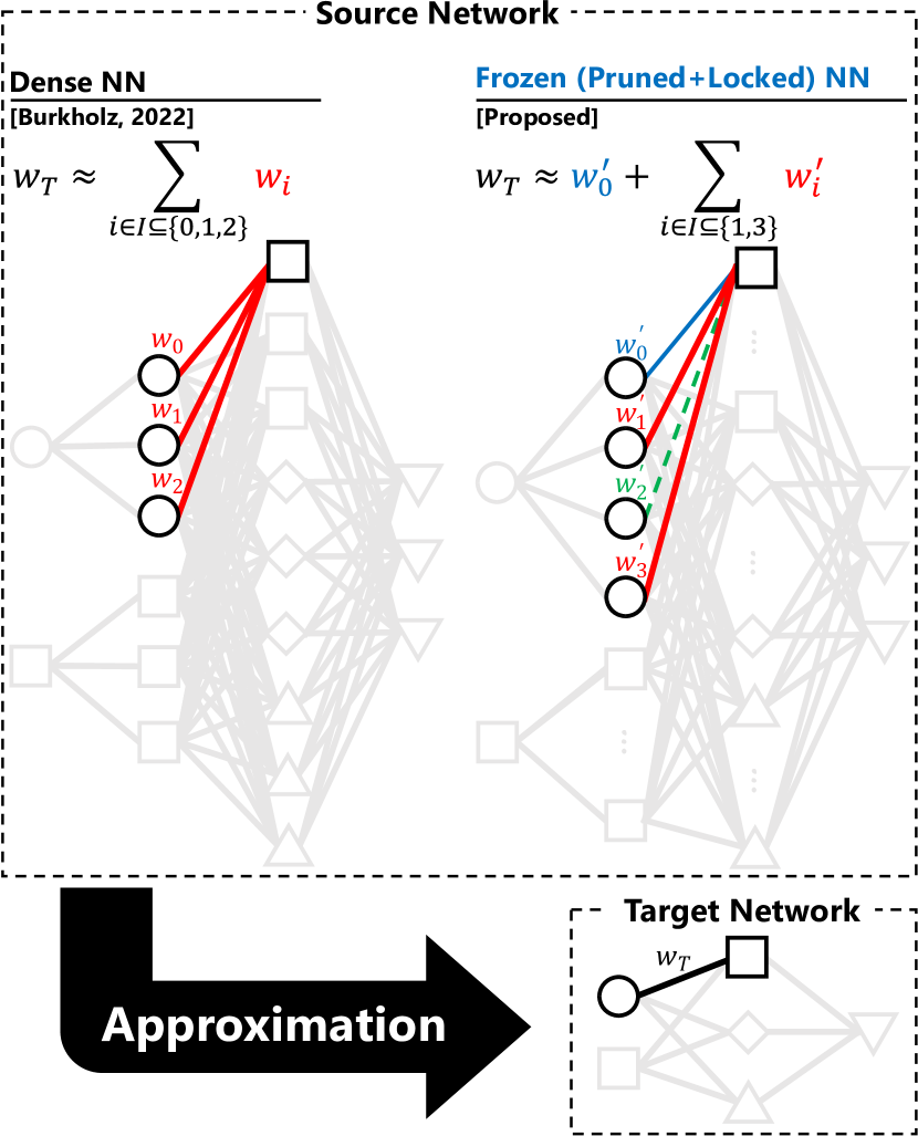
Figure 2: Burkholz (2022a) proved that target network of depth $L$ can be stochastically approximated by an SLT of depth $L\!+\!1$ by approximating each target weights ($w_{T}$) by a subset-sum of the source weights. We extend this proof to frozen source networks by solving the subset-sum approximation with some source parameters that are either unavailable ($w^{\prime}_{2}$) or must be used for the subset-sum ($w^{\prime}_{0}$).

2 Preliminaries

After outlining the background on strong lottery tickets (SLTs) and their search algorithms, this section recapitulates the subset-sum approximation technique for the existence proof of SLTs (Pensia et al., 2020; da Cunha et al., 2021; Burkholz, 2022b, a) and its extension to sparse random networks (Gadhikar et al., 2023), which Section 3 expands to the existence of SLTs within frozen networks.

2.1 Strong Lottery Tickets in Dense Networks

SLTs (Zhou et al., 2019; Ramanujan et al., 2020; Malach et al., 2020) are subnetworks within a randomly weighted neural network that achieve high accuracy without any weight training. Compared with learned dense weight models, SLTs can be reconstructed from a small amount of information: since the random weights can be regenerated from their seed, it is only necessary to store the binary supermask and the seed (Hirose et al., 2022). Instead of updating weights, SLT search algorithms for deep neural networks (Ramanujan et al., 2020; Zhou et al., 2021; Sreenivasan et al., 2022) use backpropagation to update weight scores, which are then used to generate the supermask. For example, the Edge-Popup algorithm (Ramanujan et al., 2020; Sreenivasan et al., 2022), used in this paper, finds SLTs by applying a supermask generated by from the connections with the top-$k\%$ scores. The need to keep scores in addition to the weights, and the sorting of scores necessary for generating the supermask make the computational cost of Edge-Popup slightly higher than conventional weight training.

2.2 SLT Existence via Subset-Sum Approximation

Given a set of random variables and a target value, the subset-sum problem consists on finding a subset whose total value approximates the target. Lueker (1998) showed that such subset exists with high probability if the number of random variables is sufficiently large:

Lemma 2.1 (Subset-Sum Approximation (Lueker, 1998)).

Let $X_{1},...,X_{n}\sim U(-1,1)$ be independent, uniformly distributed random variables. Then, except with exponentially small probability, any $z\in[-1,1]$ can be approximated by a subset-sum of $X_{i}$ if $n$ is sufficiently large.

Based on Lemma 2.1, previous works (Pensia et al., 2020; da Cunha et al., 2021; Burkholz, 2022b, a) showed that an SLT that approximates an arbitrary target network exists in a dense source network if it is wider and deeper than the target network. For example, Burkholz (2022a) proved that a source network with depth $L\!+\!1$ and larger width than the target network contains an SLT that can approximate the target network with depth $L$. As exemplified in Figure 2 (left), to approximate a weight $w_{T}$ of the target network, the SLT uses weights $w_{0},w_{1}$, and $w_{2}$ from the source network to construct the subset-sum. Therefore, the source network is required to be sufficiently wider than the target network, as stated in Lemma 2.1.

2.3 Strong Lottery Tickets in Sparse Networks

Recently, Gadhikar et al. (2023) revealed that SLTs also exist within sparse source networks, i.e., random networks that have been randomly pruned at initialization (see Figure 1, center). In addition to their theoretical contributions, their approach offered a practical advantage: since there are less parameters available from the beginning, the search space is reduced in proportion to the initial pruning ratio. This search space reduction can be exploited for reducing the computational cost of training.

2.4 SLT Existence in Sparse Networks

To prove the existence of SLTs within sparse networks, Gadhikar et al. (2023) extended the subset-sum approximation (Lemma 2.1) to the situation where randomly chosen variables are permanently pruned at initialization:

Lemma 2.2 (Subset-Sum Approximation in Sparse Networks (Gadhikar et al., 2023)).

Let $X_{1},...,X_{n}$ be as in Lemma 2.1, and $M_{1},...,M_{n}\sim Ber(p)$ be independent, Bernoulli distributed random variables with $p\in(0,1)$.Then, except with exponentially small probability, any $z\in[-1,1]$ can be approximated by a subset-sum of $M_{i}X_{i}$ if $n$ is sufficiently large.

By applying this extended lemma instead of Lemma 2.1 to the SLT existence theorem presented by Burkholz (2022a), Gadhikar et al. (2023) proved the SLT existence in sparse networks as the following theorem:

Theorem 2.3 (SLT Existence in Sparse Networks (Gadhikar et al., 2023)).

Let a target network $f_{T}$ with depth $L$ and a sparse source network $f_{S}$ with depth $L\!+\!1$. Assume that the source network is randomly pruned with pruning ratio $p_{l}$ for each $l$-th layer. Also assume that these networks have ReLU activation function and initialized by using a uniform distribution $U[-1,1]$. Then, except with exponentially small probability, a subnetwork $f_{SLT}$ exists in the sparse source network $f_{S}$ such that $f_{SLT}$ approximates the target network $f_{T}$ if the width of $f_{S}$ is sufficiently large.

Thus, by extending the subset-sum approximation lemma, the conventional SLT existence proof can be easily extended to various network settings.

3 Strong Lottery Tickets in Frozen Networks

Although pruning at initialization provides a search space reduction, it also imposes a limitation on the sparsity range, as it can only search for SLTs with a sparsity higher than the initial pruning ratio. For example, although an initial pruning ratio of $90\%$ vastly reduces the search space, it limits the search to only SLTs sparser than $90\%$. Therefore, this reduction in search space is incompatible with exploring the whole sparsity range for optimal accuracy.

This paper proposes a novel method that reduces the search space regardless of the desired SLT sparsity to capitalize on the training cost reduction without sacrificing accuracy. We explore the existence and performance of SLTs within a frozen source network, i.e., a random network that, in addition to randomly pruned parameters, has randomly chosen parameters forced to be permanent (i.e., never pruned) part of the SLT—locked parameters (see Figure 1, right). Since freezing is performed at initialization, before the SLT search, frozen parameters do not have a score and are not eligible for exploration, thus reducing the search space. Locking allows to further reduce the parameter search without limiting the initial pruning ratio, allowing to reduce the search space even in the case of dense source networks.

This section first provides a theoretical analysis on the existence of SLTs in such a frozen network by developing a new extension of the subset-sum approximation introduced in Section 2. Then, based on this analysis, it proposes partial SLT search, a novel method for finding such SLTs with a reduced search space. In preparation for the evaluation experiments in Section 4, we also perform a preliminary investigation of the optimal settings of the proposed method.

3.1 SLT Existence in Frozen Networks

Here we provide a theoretical result that indicates that an SLT capable of approximating a target network exist in a frozen network. This is proved by extending the subset-sum approximation lemma (Lemma 2.1) to the case where some parameters are locked (for detailed proof see Appendix A).

Lemma 3.1 (Subset-Sum Approximation in Randomly Locked Networks (Lemma A.2)).

Let $X_{1},...,X_{n}$ be as in Lemma 2.1, and $M^{\prime}_{1},...,M^{\prime}_{n}\sim Ber(q)$ be independent, Bernoulli distributed random variables with $q\in(0,1)$.Then, except with exponentially small probability, any $z\in[-1,1]$ can be approximated by the sum of $\sum_{i=1}^{n}M^{\prime}_{i}X_{i}$ and a subset-sum of $(1-M^{\prime}_{i})X_{i}$ if $n$ is sufficiently large.

Then, combining Lemma 3.1 with Lemma 2.2 further extends the subset-sum approximation to the situation where some random variables are frozen (i.e., pruned or locked).

Lemma 3.2 (Subset-Sum Approximation in Frozen Networks (Lemma A.3)).

Let $X_{1},...,X_{n}$ be as in Lemma 2.1, $M_{1},...,M_{n}\sim Ber(p)$ be as in Lemma 2.2, and $M^{\prime}_{1},...,M^{\prime}_{n}\sim Ber(q)$ be as in Lemma 3.1. Then, except with exponentially small probability, any $z\in[-1,1]$ can be approximated by the sum of $\sum_{i=1}^{n}M_{i}M^{\prime}_{i}X_{i}$ and a subset-sum of $M_{i}(1-M^{\prime}_{i})X_{i}$ if $n$ is sufficiently large.

Finally, by applying Lemma 3.2 to the Theorem 2.5 in Gadhikar et al. (2023) instead of Lemma 2.2, it follows that an SLT, which approximates a target network, exists in frozen networks.

Theorem 3.3 (SLT Existence in Frozen Networks (Theorem A.4)).

Let a target network $f_{T}$ with depth $L$ and a partially frozen source network $f_{S}$ with depth $L\!+\!1$ be given. Assume that the source network is randomly frozen with pruning ratio $p_{l}$ and locking ratio $q_{l}$ for each $l$-th layer. Also assume that these networks have ReLU activation function and initialized by using a uniform distribution $U[-1,1]$. Then, except with exponentially small probability, a subnetwork $f_{SLT}$ exists in the frozen source network $f_{S}$ such that $f_{SLT}$ approximates the target network $f_{T}$ if the width of $f_{S}$ is sufficiently large.

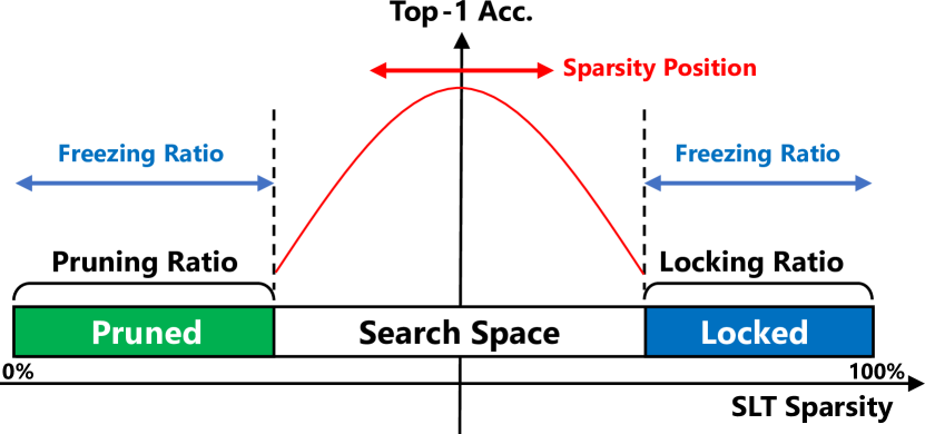
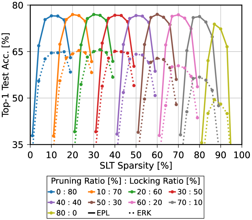
Figure 3: Pruning and locking set the bounds of the search space, whose optimal position is investigated.

Figure 4: Comparison of different prune:lock proportions of a $80\%$ freezing ratio using a Conv6 on CIFAR-${10}$.

(a)

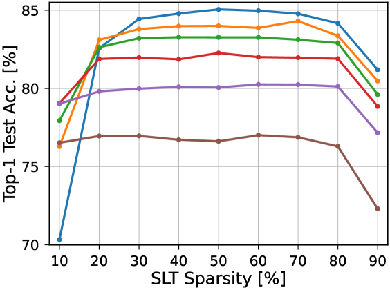
(a)

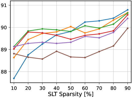
(b)

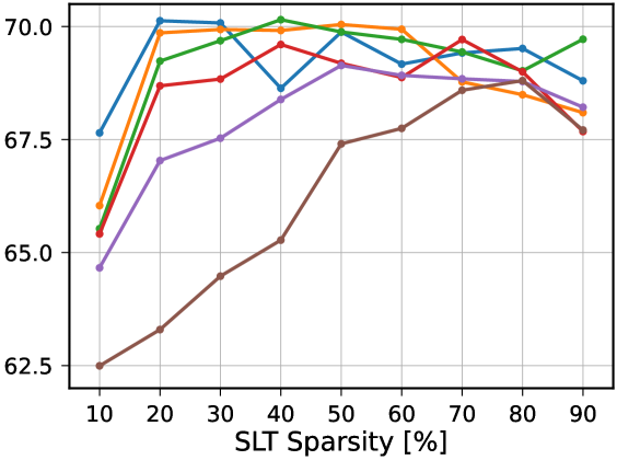
(c)

Figure 5: Impact of the freezing ratio on different architectures. Pruning and locking ratios are set following Section 3.3.

3.2 Partial SLT Search in Frozen Networks

This paper proposes a novel method for searching SLTs within frozen networks: partial SLT search. It only searches in part of the source network, as it has been pruned at initialization; and it only searches for part of the final SLT, as some of its parameters are predefined by locking.

Figure 4 illustrates how network freezing reduces the search space. The total amount of frozen parameters is determined by a global freezing ratio $F_{r}$, which is the sum of the respective pruning ratio $P_{r}$ and locking ratio $L_{r}$. Therefore, the SLT search space $S$ is formed by the $1\!-\!F_{r}$ non-frozen parameters of the original dense network. As explained previously, it is not possible to search for an SLT with a lower sparsity (denser) than the source network. Consequently, the pruning ratio sets the lower bound of the search space. On the other hand, it is not possible to search for an SLT that prunes more parameters than available, so the locking ratio sets the upper bound of the search space. (Specifically, the upper bound is given by $1\!-\!F_{r}$ .) Thus, these ratios allow to freely control the size and position of the search space over the SLT sparsity spectrum.

Frozen network construction:

We assume that the $l$-th layer of network with depth $L$ has weights $\bm{w}^{(l)}\in\mathbb{R}^{n^{(l)}}$. The number of frozen parameters is determined by the layer-wise freezing ratios $p_{f}^{(1)},...,p_{f}^{(L)}$, where each $p_{f}^{(l)}$ is defined as the sum of the layer-wise pruning ratio $p_{p}^{(l)}$ and the layer-wise locking ratio $p_{l}^{(l)}$, and $p_{f}^{(l)},p_{p}^{(l)},p_{l}^{(l)}\in[0,1]$.

To prune $p_{f}^{(l)}n^{(l)}$ parameters and lock $p_{l}^{(l)}n^{(l)}$ parameters, we generate two random masks, a pruning mask $\bm{m}^{(l)}_{p}\in\{0,1\}^{n^{(l)}}$ and a locking mask $\bm{m}^{(l)}_{l}\in\{0,1\}^{n^{(l)}}$, so that they satisfy $||1-\bm{m}^{(l)}_{p}||=p_{p}^{(l)}n^{(l)}$, $||\bm{m}^{(l)}_{l}||=p_{l}^{(l)}n^{(l)}$, and $(1-\bm{m}^{(l)}_{p})\cdot\bm{m}^{(l)}_{l}=0$ (i.e., we require pruning and locking to be implemented without overlap). The layer-wise weights frozen with these masks are calculated as

$$\bm{w}^{(l)}_{f} :=(\bm{m}_{p}^{(l)}\odot(1-\bm{m}_{l}^{(l)})+\bm{m}_{l}^{(l)})\odot\bm{w}^{(l)}.$$ (1)

These masks are fixed during training, and we search for SLTs only in the parts where $\bm{m}_{p}^{(l)}\odot(1-\bm{m}_{l}^{(l)})$ is one.

Setting the layer-wise ratios:

Our method considers the following two existing strategies for determining the layer-wise pruning ratio from the desired global pruning ratio of the source network:

• Edge Per Layer (EPL): Each layer’s pruning ratio is set so that they all have the same number of remaining weights (Price & Tanner, 2021; Gadhikar et al., 2023).

• Erdős-Rényi-Kernel (ERK): The pruning ratio of layer $l$ is proportional to the scale $(C_{in}^{(l)}+C_{out}^{(l)}+k_{h}^{(l)}+k_{w}^{(l)})/(C_{in}^{(l)}\times C_{out}^{(l)}\times k_{h}^{(l)}\times k_{w}^{(l)})$, where $C_{in}^{(l)}$, $C_{out}^{(l)}$, $k_{h}^{(l)}$, and $k_{w}^{(l)}$ denote input channels, output channels, kernel height, and kernel width of the layer $l$, respectively (Evci et al., 2020).

The same strategy is employed to determine the layer-wise pruning and freezing ratios from their respective global ratios, and then locking ratios are calculated as the difference between the corresponding freezing and pruning ratios.

Freezing mask compression:

The freezing pattern can be encoded during inference as a ternary mask—a freezing mask—that indicates whether a parameter is pruned, locked, or part of the supermask. For example, encoding pruning as $-1$, locking as $+1$, and supermask inclusion as $0$, the layer-wise freezing mask can be encoded as $\bm{m}^{(l)}_{l}+(\bm{m}^{(l)}_{p}-1)$. Since this freezing mask is also random and fixed, it can be regenerated from its seed and ratios, similarly to the random weights. Furthermore, the supermask size is reduced by excluding from it the frozen parameters, so the SLTs found by this method can be compressed in inference to an even smaller memory size than those produced by the existing SLT literature (Hirose et al., 2022; Okoshi et al., 2022; López García-Arias et al., 2023).

3.3 Optimal Positioning of the Search Space

Here we perform a preliminary investigation of the optimal positioning for each given desired SLT sparsity by exploring different pruning:locking proportions with a fixed freezing ratio of the network. Figure 4 explores different configurations of a $80\%$ freezing ratio—a search space size of $20\%$ of the original dense source network—on a Conv6 network and compares the performance of the found SLTs on CIFAR-${10}$. As expected, the best-performing SLT of each prune:lock configuration is found at the center of the search space, which maximizes the number of candidate subnetworks. In other words, within a search space size $S$, the optimal SLT sparsity is $k=P_{r}+S/2$, where $P_{r}=\frac{\sum_{l}p^{(l)}_{p}n^{(l)}}{\sum_{k}n^{(k)}}$ is the global pruning ratio of the network. Conversely, for a given freezing ratio $F_{r}$ of the network and a desired SLT sparsity $k$, the optimal search space position is set by the pruning ratio $P_{r}=k-(1-F_{r})/2$ and the corresponding locking ratio $L_{r}=F_{r}-P_{r}$. In the cases where this would result in $P_{r}\!<\!0$ or $L_{r}\!<\!0$, we choose a best-effort approach that keeps the desired freezing ratio and sets the search space bounds to $P_{r}\!=\!0$ or $L_{r}\!=\!0$, respectively.

Additionally, Figure 4 compares the two strategies for setting ratios considered in Section 3.2, showing that EPL outperforms ERK in all cases. Consequently, hereafter the proposed method sets the global ratios in order to position the search space center as close as possible to the desired SLT sparsity, and then sets the layer-wise ratios using EPL.

(a)

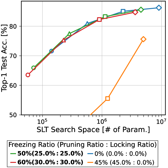
(a)

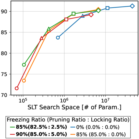
(b)

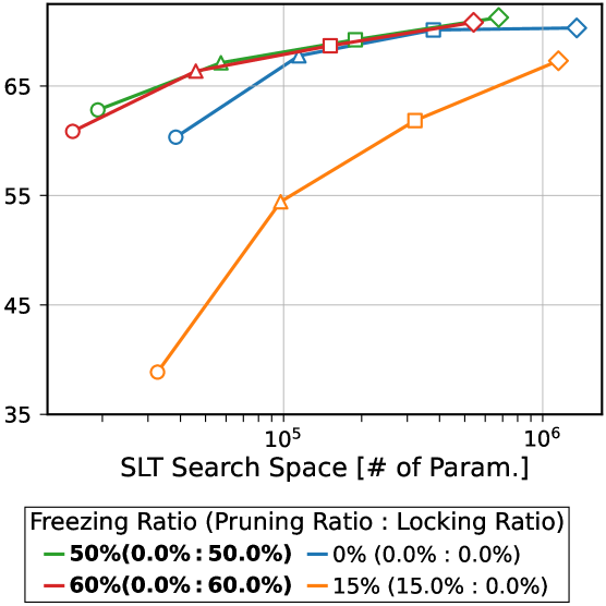
(c)

Figure 6: Freezing achieves better accuracy to search space trade-off compared to sparse ($\bullet$) or dense ($\bullet$) source networks. SLT sparsity set according to highest accuracy in Figure 5 with dense source networks.

4 Experiments

This section demonstrates that partial SLT search reduces the search space in a broad range of situations by evaluating it on image classification and node classification. We evaluate the impact of the freezing ratio on various network architectures, identifying three scenarios. Then, we explore trade-offs between accuracy, search space size, and model memory size for different network widths.

4.1 Experimental Settings

The proposed partial SLT search is evaluated on image classification using the CIFAR-${10}$ (Krizhevsky, 2009) dataset, and on node classification using the OGBN-Arxiv (Hu et al., 2020) dataset. CIFAR-${10}$ train data is split into training and validation sets with a 4:1 ratio, while for OGBN-Arxiv we use the default set split. We test the models with the best validation accuracy, and report the mean of three experiment repetitions.

For image classification we employ the VGG-like Conv6 (Simonyan & Zisserman, 2014; Ramanujan et al., 2020) and ResNet-${18}$ (He et al., 2016) architectures, and for graph node classification the GIN (Xu et al., 2019) architecture constructed with 4 layers modified by Huang et al. (2022), all implemented with no learned biases. ResNet-${18}$ and GIN use non-affine Batch Normalization (Ioffe & Szegedy, 2015), while Conv6 has no normalization layers. Random weights are initialized with the Kaiming Uniform distribution, while weight scores are initialized with the Kaiming Normal distribution (He et al., 2015).

SLTs are searched using an extension of Edge-Popup (Ramanujan et al., 2020) that enforces the desired sparsity globally instead of per-layer (Sreenivasan et al., 2022). On CIFAR-${10}$, scores are optimized for $100$ epochs using stochastic gradient descent (SGD) with momentum $0.9$, batch size $128$, weight decay $0.0001$, and initial learning rates of $0.01$ and $0.1$ for Conv6 and ResNet-${18}$, respectively. On OBGN-Arxiv, scores are optimized for $400$ epochs using AdamW (Loshchilov & Hutter, 2019) with weight decay $0.0001$ and initial learning rate $0.01$. All experiments use cosine learning rate decay (Loshchilov & Hutter, 2017).

(a)

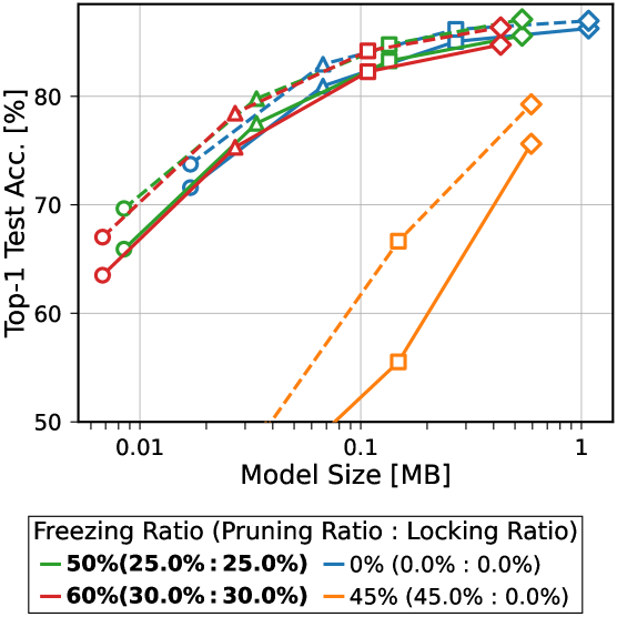
(a)

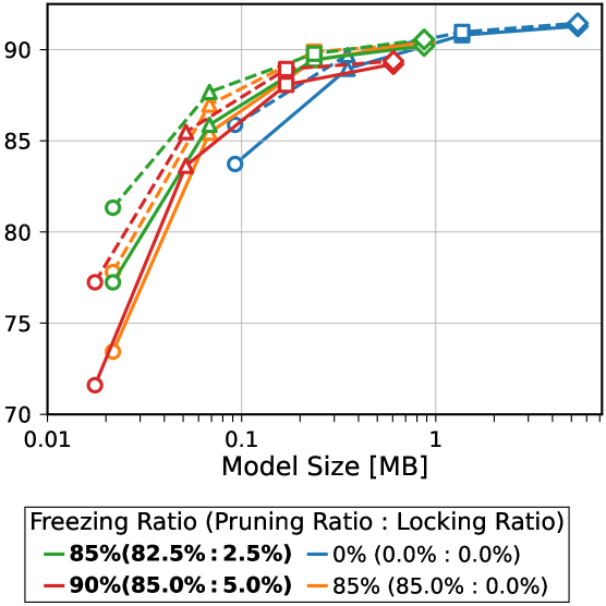
(b)

(c)

Figure 7: Freezing achieves better accuracy to memory size trade-off compared to sparse ($\bullet$) or dense ($\bullet$) source networks.

4.2 Reducing the Search Space with Freezing

An experiment is first conducted to investigate the effect of the freezing ratio of the network on SLT accuracy. We identify three scenarios, represented in Figure 5.

In the cases where the optimal SLT sparsity is found at intermediate sparsity—e.g., around $50\%$ for Conv6 in LABEL:fig:sparsity_acc_conv6—pruning and locking can be applied with equally high ratios. Results show that the search space can be reduced by $40\%$ with small impact on accuracy, and by $70\%$ with still a moderate accuracy drop of $5$ points.

Applying the much larger ResNet-${18}$ to the same task results in much stronger overparametrization. Therefore, optimal SLTs are found in the higher sparsity range, as revealed by LABEL:fig:sparsity_acc_resnet18, benefiting of much higher pruning than locking. Even in this scenario, $90\%$ sparse SLTs found in frozen networks achieve similar accuracy ($<1$ point difference) while reducing the search space by as much as $80\%$.

As an example of the scenario where optimal SLT sparsities are found in the denser range, benefitting from a higher locking ratio, we evaluate GIN in LABEL:fig:sparsity_acc_gin. Compared with the best-performing SLT found in the dense GIN, of $70.1\%$ accuracy and $20\%$ sparsity, by freezing $50\%$ of the search space our method finds better performing SLTs of $70.2\%$ accuracy with $40\%$ sparsity.

These results suggest that parameter freezing at an appropriate ratio has the effect of eliminating local optimal solutions from the search space. It is known that Edge-Popup struggles to find the SLTs of the global optimal solution (Fischer & Burkholz, 2022). While searching for SLTs in a dense network leads to convergence to a local optimal solution, a moderate reduction of the search space may reduce the number of less accurate local optimal solutions and facilitate convergence to a more accurate local optimal solution within the reduced search space. In other words, we conjecture that if the network is properly frozen, the local optimal solution for the reduced search space is close to the global optimal solution of the entire search space.

4.3 Accuracy to Search Space Trade-Off

Section 3 sets as a requisite of the subset-sum proof that the source network has a sufficiently larger width than the target network. Figure 5 explores varying the width of the source network to analyze its impact on accuracy and search space size. SLT sparsity is fixed to that of the best performing SLT found in a dense source network in Figure 5: $50\%$ in Conv6, $90\%$ in ResNet-${18}$, and $20\%$ in GIN.

Compared to the dense source network, the results show in all cases that, when the frozen network is twice as wide, the found SLTs for a given sparsity achieve similar or higher performance with a similar or smaller search space size. That is, the propsed method improves the accuracy to search space size trade-off. In the case of GIN in LABEL:fig:search_space_acc_gnn, the SLT found in a $2\times$ wider frozen source even achieves higher accuracy than those found in any dense source network.

As shown in LABEL:fig:search_space_acc_conv6 and LABEL:fig:search_space_acc_gnn, in the scenarios that only allow for medium to low pruning, there is a limit to the number of parameters that can be pruned for a given SLT sparsity, and only aggressive pruning leads to less accurate SLTs. By additionally locking parameters, our method reduces the search space further and finds SLTs of higher accuracy than those within sparse or dense networks for a similar search space size. Pruning only improves the trade-off in the scenario that allows higher pruning than locking, as shown in LABEL:fig:search_space_acc_resnet18, while our method improves the accuracy to search space trade-off in all scenarios.

4.4 Accuracy to Model Memory Size Trade-Off

The freezing mask compression scheme proposed in Section 3.2 allows to reduce the memory model size during inference by regenerating both the random weights and the freezing mask with a random number generator (RNG). Here we consider this compression and investigate the accuracy to model size trade-off offered by the SLTs found by the proposed method. Furthermore, considering the practical application of partial SLT search on specialized hardware, we also compare the Kaiming Uniform (KU) weight initialization used so far with the binary weights provided by the Signed Kaiming Constant (SKC) initialization (Ramanujan et al., 2020), which can be exploited for reduced computational cost in neural engines (Hirose et al., 2022). For SKC we scale weights by $1/\sqrt{1-k_{l}}$, where $k_{l}$ is the sparsity of each layer, as proposed by Ramanujan et al. (2020).

As illustrated in Figure 7, compared to the SLTs found in dense or sparse source networks, SLTs found by our method achieve similar or higher accuracy for similar or smaller model size, thus improving the accuracy to model size trade-off in all scenarios. In other words, partial SLT search not only reduces the search space during training, but also reduces the model size during inference, further improving performance over conventional SLT search methods.

Empirically, it is known that SLTs within a SKC initialized dense network achieve better performance than with continuous random weights (Ramanujan et al., 2020; Okoshi et al., 2022; López García-Arias et al., 2023; Yan et al., 2023). Our results show that such a trend can also be observed in frozen source networks. Nonetheless, in all source networks, we find that this improvement is smaller the wider the source network is, suggesting that the requirement for source networks of larger width is weaker in the case of binary weights.

Table 1: Comparison between trained-weight networks and SLTs found in dense, sparse, and frozen networks.

Conv6 & CIFAR-${10}$
Method (Source Network)	Weight Initialization	Sparsity [%]	Pruning Ratio [%]	Locking Ratio [%]	Top-1 Test Acc. [%]	Search Space [# Parameters]	Model Size [MB]
Weight Training	KU	-	-	-	$87.1$	$2.26$ M	$8.63$
SLT (Dense)	SKC	$50$	$0$	$0$	$86.2$	$2.26$ M	$0.27$
SLT (Sparse)	SKC	$50$	$45$	$0$	$66.7$	$1.24$ M	$0.15$
SLT (Frozen)	SKC	$50$	$25$	$25$	$84.8$	$1.13$ M	$0.13$
ResNet-${18}$ & CIFAR-${10}$
Weight Training	KU	-	-	-	$92.5$	$11.16$ M	$42.63$
SLT (Dense)	SKC	$90$	$0$	$0$	$91.0$	$11.16$ M	$1.37$
SLT (Sparse)	SKC	$90$	$85$	$0$	$89.9$	$1.67$ M	$0.24$
SLT (Frozen)	SKC	$90$	$82.5$	$2.5$	$89.8$	$1.67$ M	$0.24$
SLT (Frozen)	SKC	$90$	$85$	$5$	$88.9$	$1.12$ M	$0.17$
GIN & OGBN-Arxiv
Weight Training	KU	-	-	-	$70.1$	$0.38$ M	$1.452$
SLT (Dense)	SKC	$20$	$0$	$0$	$70.1$	$0.38$ M	$0.054$
SLT (Sparse)	SKC	$20$	$15$	$0$	$63.1$	$0.32$ M	$0.047$
SLT (Frozen)	SKC	$20$	$0$	$40$	$70.6$	$0.23$ M	$0.036$

4.5 Result Analysis

Table 1 summarizes the presented results and compares the proposed method to weight training and SLT search in dense and sparse source networks for the same network architecture and SLT sparsity.

In the case of Conv6, compared to weight training our method provides reductions of $2\times$ and $66.4\times$ of the search space and model size, respectively, in exchange of a small accuracy drop. Compared to the SLT found in the sparse source network, the SLT found by partial search achieves much higher accuracy.

Even in the more challenging case of ResNet-${18}$, SLTs found in a frozen network are $250.8\times$ smaller than the trained-weight model while reducing search space by $10.0\times$. When comparing SLTs found in sparse and frozen networks with the same $85\%$ freezing ratio, the accuracy is almost equivalent, demonstrating that the inclusion of locking does not introduce a degrade in accuracy even in the scenario that benefits more from pruning.

Interestingly, the SLT found in the frozen GIN model achieves higher accuracy than the trained-weight network, even though the model size and search space are reduced by $40.3\times$ and $1.7\times$, respectively. The SLT found within a dense network also achieves comparable accuracy to the trained-weight network, but the SLT found by our method performs better and is smaller. Generally, graph neural networks (GNNs) suffer from a generalization performance degradation due to the over-smoothing problem (Li et al., 2018). Searching for SLTs within dense GNNs has been shown to mitigate the over-smoothing problem (Huang et al., 2022) and achieve higher accuracy. As our method is even more accurate than dense networks, it is possible that parameter freezing offers an even stronger solution to the over-smoothing problem.

5 Conclusion

This paper capitalizes on the fact that pruning a randomly weighted network at initialization reduces the SLT search space, but identifies that it limits the search to a suboptimal sparsity region. This problem is tackled by freezing (i.e., pruning or locking) some parameters at initialization, excluding them from the search. Freezing allows to search for SLTs efficiently in the optimal sparsity range, while further reducing search space during training and model size during inference. Experimental results show that SLTs found in frozen networks improve the accuracy to search space and accuracy to model size trade-offs compared to SLTs found in dense (Ramanujan et al., 2020; Sreenivasan et al., 2022) or sparse source networks (Gadhikar et al., 2023). Interestingly, although for weight training random parameter locking has only been found useful for reducing accuracy degradation in network compression (Zhou et al., 2019; Wimmer et al., 2020), we identify a scenario in SLT training where it can be used for raising accuracy, even outperforming weight-trained networks. Our method can be interpreted as being capable of generating more useful SLT information from a random seed than previous methods, and as a result, it offers an opportunity for reducing off-chip memory access in specialized SLT accelerators (Hirose et al., 2022). We hope that this work will serve as a base for raising further the efficiency of SLT training and inference.

Impact Statements

This paper presents work whose goal is to advance the field of machine learning. Among the many potential societal consequences of our work, we highlight its potential to reduce the computational cost of inference and training of neural networks, and thus their energy consumption footprint.

Appendix A Proof for Strong Lottery Tickets (SLTs) Existence in Frozen Networks

This section describes the proofs of the lemma and theorem introduced in the manuscript. For reference, we present a theorem presented by Gadhikar et al. (2023) in advance.

Theorem A.1 (SLT Existence in Sparse Networks (Gadhikar et al., 2023)).

Let input data $\mathcal{D}$ , a target network $f_{T}$ with depth $L$, and a source network $f_{S}$ with depth $L+1$, parameters $\bm{\theta}_{S}$, and edge probabilities $p_{l}$ be given. Assume that these networks have ReLU activation function, and each element of $\bm{\theta}_{S}$ is uniformly distributed over $[-1,1]$. Then, with probability at least $1-\delta$, there exists a binary mask $\bm{m}_{S}$ so that each output component $i$ is approximated as $\max_{\bm{x}\in\mathcal{D}}\left\|f_{T,i}(\bm{x})-f_{S,i}(\bm{x};\bm{\theta}_{S}\odot\bm{m}_{S})\right\|<\epsilon$ if

$$n_{S,l}\geq C\frac{n_{T,l}}{\log(1/1-p_{l+1})}\log\left(\frac{1}{\min\{\epsilon_{l},\delta/\rho\}}\right)$$ (2)

for $l\geq 1$,where

$$\epsilon_{l} \coloneqq\frac{\epsilon}{n_{T,L}L}\left[(1+B_{l-1}\left(1+\frac{\epsilon}{L}\right)\prod_{k=l+1}^{L-1}\left(\left\|\bm{\theta}_{T}^{(l)}\right\|_{\infty}+\frac{\epsilon}{L}\right)\right]^{-1},$$ (3)

$$B_{l} \coloneqq\sup_{\bm{x}\in\mathcal{D}}\left\|\bm{x}_{T}^{(l)}\right\|_{1},$$ (4)

$$\rho =\frac{CN_{T}^{1+\gamma}}{\log\left(1/(1-\min_{l}\{p_{l}\})\right)^{1+\gamma}}\log\left(\frac{1}{\min\{\min_{l}\{\epsilon_{l}\},\delta\}}\right)$$ (5)

for any $\gamma\geq 0$. Moreover, we need to satisfy

$$n_{S,0}\geq Cd\log\left(\frac{1}{\min\left\{\epsilon_{1},\delta/\rho\right\}}\right),$$ (6)

where $C>0$ denotes a generic constant that is independent of $n_{T,l},L,p_{l},\delta$, and $\epsilon$.

We first extend the lemma of the subset-sum approximation shown by Lueker (1998) to the case where some random variables are always included in the subset-sum.

Lemma A.2 (Subset-Sum Approximation in Randomly Locked Networks).

Let $X_{1},\cdots,X_{n}\sim U(-1,1)$ be independent, uniformly distributed random variables, and $M_{1},\cdots,M_{n}\sim\mathrm{Ber}(q)$ be independent, Bernoulli distributed random variables with $q\in(0,1)$. Let $\varepsilon,\delta>0$. Then, with probability at least $1-\delta$, for any $z\in[-1,1]$, there exists indices $I\subset\{1,\cdots,n\}$ such that $|z-\sum_{i=1}^{n}M_{i}X_{i}-\sum_{i\in I}(1-M_{i})X_{i}|\leq\varepsilon$ if

$$n\geq C\log\left(\frac{8}{\varepsilon\delta}\right),$$ (7)

where $C>0$ is a constant.

Proof.

Let $M_{1},\cdots,M_{n}\sim\mathrm{Ber}(q)$ and $m:=\sum_{i}M_{i}$. By Hoeffding’s inequality, we have

$$\mathbb{P}\left(|m-qn|\leq\varepsilon_{M}n\right)\geq 1-2\exp\left(-\frac{\varepsilon_{M}^{2}n}{2q(1-q)}\right)$$ (8)

for $\varepsilon_{M}>0$. Thus, if we set $n\geq\frac{2q(1-q)\log(2/\delta)}{\varepsilon_{M}^{2}}$ and $\varepsilon_{M}:=\frac{\min(q,1-q)}{2}$, we have

$$(2q-\beta)n\leq m\leq\beta n$$ (9)

with $\beta:=q+\varepsilon_{M}=\min(\frac{3q}{2},\frac{1+q}{2})\in(0,1)$, with probability at least $1-\delta$. In particular, the number of non-vanishing terms in the sum $\sum_{i\in I}(1-M_{i})X_{i}$ is $n-m\geq(1-\beta)n$ as long as each $X_{i}$ is non-zero.

Now fix $M_{1},\cdots,M_{n}\sim\mathrm{Ber}(q)$ with $(2q-\beta)n\leq m\leq\beta n$. The goal is to approximate $z\in[-1,1]$ and $\sum_{i=1}^{n}M_{i}X_{i}$ by subset sum from $\{(1-M_{i})X_{i}:M_{i}=0\}$. For simplicity, we split it into two parts:

$$\{(1-M_{i})X_{i}:M_{i}=0\}=\{X^{\prime}_{1},\cdots,X^{\prime}_{n_{1}}\}\cup\{X^{\prime\prime}_{1},\cdots,X^{\prime\prime}_{n_{2}}\},$$ (10)

where the former part is used for approximating $z\in[-1,1]$ and the latter part for approximating $\sum_{i=1}^{n}M_{i}X_{i}$.

To approximate $z\in[-1,1]$, we can directly apply Corollary 2.5 from Lueker (1998):

$$\mathbb{P}\left(\forall z\in\left[-1,1\right],\exists I\subset\{1,\cdots,n_{1}\}\text{ s.t. }|z-\sum_{i\in I}X^{\prime}_{i}|\geq\varepsilon\right)\geq 1-\delta$$ (11)

whenever $n_{1}\geq C\log(2/\varepsilon\delta)$.

To approximate $\sum_{i=1}^{n}M_{i}X_{i}$, we have to evaluate its norm. By Hoeffding’s inequality on $X_{i}$’s with $M_{i}\not=0$, we have

$$\mathbb{P}\Big{(}\Big{|}\sum_{i=1}^{n}M_{i}X_{i}\Big{|}\leq\alpha m\Big{)}\geq 1-2\exp\left(-\frac{3\alpha^{2}m}{2}\right),$$ (12)

for any fixed $\alpha>0$, whose value will be specified later. Thus $\Big{|}\sum_{i=1}^{n}M_{i}X_{i}\Big{|}\leq\alpha m\leq\alpha\beta n$ holds with probability at least $1-\delta$ whenever $m\geq\frac{2\log(2/\delta)}{3\alpha^{2}}$. Since $m\leq\beta n$ holds, $n\geq\frac{2\log(2/\delta)}{3\alpha^{2}\beta}$ is enough.

From the proof of Corollary 3.1 in Lueker (1998), for any $\gamma\in(0,\frac{1}{4})$, we know that

$$\mathbb{P}\left(\forall z\in\left[-\gamma n_{2},\gamma n_{2}\right],\exists I\subset\{1,\cdots,n_{2}\}\text{ s.t. }|z-\sum_{i\in I}X^{\prime\prime}_{i}|\geq\varepsilon\right)$$ (13)

$$\geq 1-\delta-2\exp\left(-\frac{(1-4\gamma)^{2}n_{2}}{64}\right)$$ (14)

whenever $n_{2}\geq C\log(\frac{2}{\varepsilon\delta})$. Thus if

$$n_{2}\geq\max\left(C\log(\frac{2}{\varepsilon\delta}),\frac{C^{\prime}}{(1-4\gamma)^{2}}\log(\frac{2}{\delta})\right)$$ (15)

holds, we can approximate any $z\in[-\gamma n_{2},\gamma n_{2}]$ by subset sum of $X^{\prime\prime}_{1},\cdots,X^{\prime\prime}_{n_{2}}$ with probability $1-2\delta$.

Now we assume $(\alpha\beta/\gamma)n\leq n_{2}$. For example, if we set $\alpha=\frac{1}{10}$ and $\gamma=\frac{1}{5}$, the assumption is satisfied when we split $\{(1-M_{i})X_{i}\}$ by $n_{1}=n_{2}=\frac{n}{2}$ in (10). Then the approximation (13) can be applied to $z=\sum_{i=1}^{n}M_{i}X_{i}$ with high probability since $|\sum_{i=1}^{n}M_{i}X_{i}|\leq\alpha m\leq\alpha\beta n\leq\gamma n_{2}$ holds.

By combining (11), (12), (15) with the fact that $n=m+n_{1}+n_{2}$, and replacing $\delta$ with $\delta/4$, we obtain the desired results. ∎

By similar arguments as in Lueker (1998) or Pensia et al. (2020), we can easily generalize Lemma A.2 to the case where the distribution followed by $X_{i}$ contains the uniform distribution. Also, by combining our proof and the proof of Lemma 2.4 in Gadhikar et al. (2023), we can prove the following extension of Lemma A.2:

Lemma A.3 (Subset-Sum Approximation in Frozen Networks.).

Let $X_{1},...,X_{n}$ be independent, uniformly distributed random variables so that $X\sim U(-1,1)$, $M_{1},...,M_{n}$ be independent, Bernoulli distributed random variables so that $M_{i}\sim Ber(p)$ for $p\in(0,1)$, and $M^{\prime}_{1},...,M^{\prime}_{n}$ be independent, Bernoulli distributed random variables so that $M^{\prime}_{i}\sim Ber(q)$ for $q\in(0,1)$. Let $\epsilon,\delta\in(0,1)$ given. Then for any $z\in[-1,1]$ there exists a subset $I\subseteq\{1,...,n\}$ so that with probability at least $1-\delta$ we have $\left|z-\sum_{i=1}^{n}M_{i}M^{\prime}_{i}X_{i}-\sum_{i\in I}M_{i}\left(1-M^{\prime}_{i}\right)X_{i}\right|\leq\epsilon$ if

$$n\geq C\log\left(\frac{C^{\prime}}{\varepsilon\delta}\right),$$ (16)

where $C,C^{\prime}>0$ is a constant.

Theorem A.4 (SLT Existence in Frozen Networks).

Let $\mathcal{D}$ be input data, $f_{T}$ be a target network with depth $L$, and $f_{S}$ be a source network with depth $L+1$, $\bm{\theta}_{S}$ be a parameter of $f_{S}$, and $p_{l},q_{l}\in(0,1)$. Assume that these networks have ReLU activation function, and each element of $\bm{\theta}_{S}$ is uniformly distributed over $[-1,1]$. Also assume that $\bm{\theta}_{S}$ is randomly pruned and locked with pruning ratio $p_{l}$ and locking ratio $q_{l}$ for each $l$-th layer. Then, with probability at least $1-\delta$, there exists a binary mask $\bm{m}_{S}$ so that each output component $i$ is approximated as $\max_{\bm{x}\in\mathcal{D}}\left\|f_{T,i}(\bm{x})-f_{S,i}(\bm{x};\bm{\theta}_{S}\odot\bm{m}_{S})\right\|<\epsilon$ if

$$n_{S,l} \geq C_{1}\log\left(\frac{C_{2}}{\min\{\epsilon_{l},\delta/\rho\}}\right)n_{T,l}, (l\geq 1)$$ (17)

$$n_{S,0} \geq C_{3}\log\left(\frac{C_{4}}{\min\left\{\epsilon_{1},\delta/\rho\right\}}\right)d (l=0)$$ (18)

where $C_{i}>0$ are constants that include $p_{l},q_{l}$, and $\rho,\epsilon_{l}$ are as defined in Theorem A.1.

Proof.

By replacing Lemma 2.4 in Gadhikar et al. (2023) with our Lemma A.3, we obtain the desired result as an extension of Theorem 2.5 in Gadhikar et al. (2023). ∎

References

- Burkholz (2022a) Burkholz, R. Most activation functions can win the lottery without excessive depth. Proc. Adv. Neural Inform. Process. Syst., 35:18707–18720, 2022a.
- Burkholz (2022b) Burkholz, R. Convolutional and residual networks provably contain lottery tickets. In Proc. Int. Conf. Mach. Learn., pp. 2414–2433. PMLR, 2022b.
- Burkholz et al. (2022) Burkholz, R., Laha, N., Mukherjee, R., and Gotovos, A. On the existence of universal lottery tickets. In Proc. Int. Conf. Learn. Repr., 2022.
- da Cunha et al. (2021) da Cunha, A., Natale, E., and Viennot, L. Proving the lottery ticket hypothesis for convolutional neural networks. In Proc. Int. Conf. Learn. Repr., 2021.
- Diffenderfer & Kailkhura (2021) Diffenderfer, J. and Kailkhura, B. Multi-prize lottery ticket hypothesis: Finding accurate binary neural networks by pruning a randomly weighted network. In Proc. Int. Conf. Learn. Repr., 2021.
- Evci et al. (2020) Evci, U., Gale, T., Menick, J., Castro, P. S., and Elsen, E. Rigging the lottery: Making all tickets winners. In Proc. Int. Conf. Mach. Learn., pp. 2943–2952. PMLR, 2020.
- Ferbach et al. (2023) Ferbach, D., Tsirigotis, C., Gidel, G., and Bose, J. A general framework for proving the equivariant strong lottery ticket hypothesis. In Proc. Int. Conf. Learn. Repr., 2023.
- Fischer & Burkholz (2022) Fischer, J. and Burkholz, R. Plant ’n’ seek: Can you find the winning ticket? In Proc. Int. Conf. Learn. Repr., 2022.
- Gadhikar et al. (2023) Gadhikar, A. H., Mukherjee, S., and Burkholz, R. Why random pruning is all we need to start sparse. In Proc. Int. Conf. Mach. Learn., pp. 10542–10570. PMLR, 2023.
- He et al. (2015) He, K., Zhang, X., Ren, S., and Sun, J. Delving deep into rectifiers: Surpassing human-level performance on ImageNet classification. In Proc. IEEE Int. Conf. Comput. Vis., pp. 1026–1034, 2015.
- He et al. (2016) He, K., Zhang, X., Ren, S., and Sun, J. Deep residual learning for image recognition. In Proc. IEEE Comput. Soc. Conf. Comput. Vis. and Pattern Recognit., pp. 770–778, 2016.
- Hirose et al. (2022) Hirose, K., Yu, J., Ando, K., Okoshi, Y., López García-Arias, Á., Suzuki, J., Van Chu, T., Kawamura, K., and Motomura, M. Hiddenite: 4K-PE hidden network inference 4D-tensor engine exploiting on-chip model construction achieving 34.8-to-16.0 TOPS/W for CIFAR-100 and ImageNet. In Proc. IEEE Int. Solid-State Circuits Conf., volume 65, pp. 1–3. IEEE, 2022.
- Hu et al. (2020) Hu, W., Fey, M., Zitnik, M., Dong, Y., Ren, H., Liu, B., Catasta, M., and Leskovec, J. Open graph benchmark: Datasets for machine learning on graphs. Proc. Adv. Neural Inform. Process. Syst., 33:22118–22133, 2020.
- Huang et al. (2022) Huang, T., Chen, T., Fang, M., Menkovski, V., Zhao, J., Yin, L., Pei, Y., Mocanu, D. C., Wang, Z., Pechenizkiy, M., and Liu, S. You can have better graph neural networks by not training weights at all: Finding untrained GNNs tickets. In Learn. of Graphs Conf., 2022.
- Ioffe & Szegedy (2015) Ioffe, S. and Szegedy, C. Batch normalization: Accelerating deep network training by reducing internal covariate shift. In Proc. Int. Conf. Mach. Learn., pp. 448–456. pmlr, 2015.
- Krizhevsky (2009) Krizhevsky, A. Learning multiple layers of features from tiny images. Master’s thesis, Department of Computer Science, University of Toronto, Toronto, 2009.
- Li et al. (2018) Li, Q., Han, Z., and Wu, X.-M. Deeper insights into graph convolutional networks for semi-supervised learning. In Proc. AAAI Conf. on Artif. Intell., volume 32, 2018.
- López García-Arias et al. (2023) López García-Arias, Á., Okoshi, Y., Hashimoto, M., Motomura, M., and Yu, J. Recurrent residual networks contain stronger lottery tickets. IEEE Access, 11:16588–16604, 2023. doi: 10.1109/ACCESS.2023.3245808.
- Loshchilov & Hutter (2017) Loshchilov, I. and Hutter, F. SGDR: Stochastic gradient descent with warm restarts. In Proc. Int. Conf. Learn. Repr., 2017.
- Loshchilov & Hutter (2019) Loshchilov, I. and Hutter, F. Decoupled weight decay regularization. In Proc. Int. Conf. Learn. Repr., 2019.
- Lueker (1998) Lueker, G. S. Exponentially small bounds on the expected optimum of the partition and subset sum problems. Random Struct. Algor., 12(1):51–62, 1998.
- Malach et al. (2020) Malach, E., Yehudai, G., Shalev-Schwartz, S., and Shamir, O. Proving the lottery ticket hypothesis: Pruning is all you need. In Proc. Int. Conf. Mach. Learn., pp. 6682–6691. PMLR, 2020.
- Okoshi et al. (2022) Okoshi, Y., López García-Arias, Á., Hirose, K., Ando, K., Kawamura, K., Van Chu, T., Motomura, M., and Yu, J. Multicoated supermasks enhance hidden networks. In Proc. Int. Conf. Mach. Learn., pp. 17045–17055, 2022.
- Orseau et al. (2020) Orseau, L., Hutter, M., and Rivasplata, O. Logarithmic pruning is all you need. Proc. Adv. Neural Inform. Process. Syst., 33:2925–2934, 2020.
- Pensia et al. (2020) Pensia, A., Rajput, S., Nagle, A., Vishwakarma, H., and Papailiopoulos, D. Optimal lottery tickets via subset sum: Logarithmic over-parameterization is sufficient. Proc. Adv. Neural Inform. Process. Syst., 33:2599–2610, 2020.
- Price & Tanner (2021) Price, I. and Tanner, J. Dense for the price of sparse: Improved performance of sparsely initialized networks via a subspace offset. In Proc. Int. Conf. Mach. Learn., pp. 8620–8629. PMLR, 2021.
- Ramanujan et al. (2020) Ramanujan, V., Wortsman, M., Kembhavi, A., Farhadi, A., and Rastegari, M. What’s hidden in a randomly weighted neural network? In Proc. IEEE Comput. Soc. Conf. Comput. Vis. and Pattern Recognit., pp. 11893–11902, 2020.
- Simonyan & Zisserman (2014) Simonyan, K. and Zisserman, A. Very deep convolutional networks for large-scale image recognition. arXiv preprint arXiv:1409.1556, 2014.
- Sreenivasan et al. (2022) Sreenivasan, K., Sohn, J., Yang, L., Grinde, M., Nagle, A., Wang, H., Xing, E., Lee, K., and Papailiopoulos, D. Rare gems: Finding lottery tickets at initialization. Proc. Adv. Neural Inform. Process. Syst., 35:14529–14540, 2022.
- Wimmer et al. (2020) Wimmer, P., Mehnert, J., and Condurache, A. Freezenet: Full performance by reduced storage costs. In Proc. Asian Conf. Comput. Vis., 2020.
- Xu et al. (2019) Xu, K., Hu, W., Leskovec, J., and Jegelka, S. How powerful are graph neural networks? In Proc. Int. Conf. Learn. Repr., 2019.
- Yan et al. (2023) Yan, J., Ito, H., López García-Arias, Á., Okoshi, Y., Otsuka, H., Kawamura, K., Chu, T. V., and Motomura, M. Multicoated and folded graph neural networks with strong lottery tickets. In Learn. of Graphs Conf., 2023.
- Yeo et al. (2023) Yeo, S., Jang, Y., Sohn, J., Han, D., and Yoo, J. Can we find strong lottery tickets in generative models? In Proc. AAAI Conf. on Artif. Intell., volume 37, pp. 3267–3275, 2023.
- Zhou et al. (2019) Zhou, H., Lan, J., Liu, R., and Yosinski, J. Deconstructing lottery tickets: Zeros, signs, and the supermask. Proc. Adv. Neural Inform. Process. Syst., 32, 2019.
- Zhou et al. (2021) Zhou, X., Zhang, W., Xu, H., and Zhang, T. Effective sparsification of neural networks with global sparsity constraint. In Proc. IEEE Comput. Soc. Conf. Comput. Vis. and Pattern Recognit., pp. 3599–3608, 2021.