Performance Evaluation and Analysis of Thresholding-based Interference Mitigation for Automotive Radar Systems

Abstract

In automotive radar, time-domain thresholding (TD-TH) and time-frequency domain thresholding (TFD-TH) are crucial techniques underpinning numerous interference mitigation methods. Despite their importance, comprehensive evaluations of these methods in dense traffic scenarios with different types of interference are limited. In this study, we segment automotive radar interference into three distinct categories. Utilizing the in-house traffic scenario and automotive radar simulator, we evaluate interference mitigation methods across multiple metrics: probability of detection, signal-to-interference-plus-noise ratio, and phase error involving hundreds of targets and dozens of interfering radars. The numerical results highlight that TFD-TH is more effective than TD-TH, particularly as the density and signal correlation of interfering radars escalate.

Index Terms—  Automotive radar, interference mitigation, time-frequency analysis, CFAR detection

1 Introduction

Radar-to-radar interference refers to undesired signals coming from surrounding radars, which can deteriorate the performance of a victim radar by corrupting desired target signals. Several decades ago, when automotive radars were first available and utilized in high-end vehicles, radar interference has not been considered as a significant issue given their limited deployment. Consequently, interference mitigation algorithms were mainly confined to basic time domain detection and processing. Today, automotive radars are ubiquitous and play an instrumental role in various advanced driver assistance system (ADAS) applications such as adaptive cruise control, autonomous emergency brake, blind spot detection, line change assistance, etc [1, 2]. The cutting-edge 4D automotive radar has further cemented its importance in the domain of autonomous driving (AD) owing to its high-resolution capability and resilience against adverse weather conditions [3, 4]. As the use of automotive radars proliferates, radar-to-radar interference is inevitable and intensifying, underscoring the pressing need for innovative interference mitigation strategies [5].

In recent years, numerous automotive radar interference mitigation methods [6, 7, 8, 9, 10, 11, 12, 13, 14, 15, 16] have been proposed by the academic and industrial communities. Central to these methods are two core techniques: time domain thresholding (TD-TH) and time-frequency domain thresholding (TFD-TH). While many advanced interference mitigation methods build upon these two techniques by incorporating additional steps after thresholding, such as interpolation to enhance signal-to-noise ratio [10, 12, 8], the crux of their performance lies in the efficacy of TD-TH and TFD-TH. The importance of TD-TH and TFD-TH is not merely due to their role as bases for advanced interference mitigation methods; it is also attributed to their inherent applicability. As interference mitigation typically precedes other signal processing steps (e.g., range, velocity, and angle estimation) in automotive radar processors, and given the real-time requirements of such systems, both techniques stand out as essential and pragmatic with their lightweight computation. However, a comprehensive comparison between them in dense traffic scenarios with different types of interference remains absent. This gap in analysis leaves the potential and advantages of time-frequency domain processing not fully explored or understood.

In this paper, we aim to bridge the gap by comparing the performance of TD-TH and TFD-TH in a more comprehensive setup compared to the prior studies. It is imperative to understand that conducting real-world experiments with dozens of moving interference sources is challenging or virtually impossible given the safety concerns involved. Thus, hundreds of targets (e.g., vehicles and guardrails) and dozens of interfering radars with various types of interference are simulated by our in-house traffic scenario simulator and high-fidelity automotive radar front end (RFE) simulator. Then, the interference mitigation performance of TD-TH and TFD-TH was evaluated in terms of probability of detection (PD) and signal-to-interference-plus-noise ratio (SINR) in the range-Doppler (RD) map level, unlike other works that did the evaluation in the range spectrum level. Furthermore, we introduce phase error cumulative distribution function (CDF) as a significant metric to evaluate the influence of interference mitigation on subsequent radar signal processing, such as angle estimation, which has been overlooked in most automotive radar interference mitigation works.

2 System Model

Consider a simple traffic scenario comprising a victim radar, an interfering radar, and a single point target. The transmitted frequency modulated continuous wave (FMCW) signal of the victim radar is given by:

$$s_{p}(t)=e^{j\pi\alpha t^{2}},\,\,0<t<T_{a},$$ (1)

where $\alpha$ is the chirp slope determined by $\alpha=\frac{B}{T_{a}}$. Here, $T_{a}$ indicates the active time duration of a single pulse, and $B$ is the chirp sweep bandwidth. Given that $M$ pulses are transmitted per coherent processing interval, the transmitted modulated signal of the victim radar can be expressed as

$$s_{\text{tx}}(t)=\sum_{m=0}^{M-1}s_{p}(t-mT_{\text{PRI}})e^{j2\pi f_{c}t},$$ (2)

where $f_{c}$ is the carrier frequency, and $T_{\text{PRI}}$ is the pulse repetition interval (PRI), combining the active and dead time ($T_{\text{PRI}}=T_{a}+T_{d}$ and $T_{d}>0$), as shown in Fig. 1. The interfering radar emits a signal, $\tilde{s}_{\text{tx}}(t)$, resembling the waveforms defined by (1) and (2), but with varied parameters. In this paper, a tilde notation will be used for interference to differentiate these parameters from those of the victim radar.

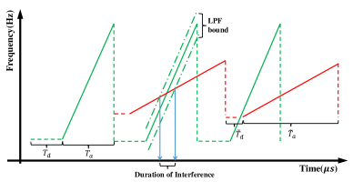
Fig. 1: Duration of interference overview. Green chirps are signals transmitted by a victim radar and red chirps are interference signals transmitted by an interfering radar.

2.1 Target Signal Model

The transmitted signal reflected back by a single target is received and demodulated at the RFE. The received signal, after passing through the mixer, can be represented by

$$\begin{split}s_{\text{rx}}(t)&=as_{\text{tx}}(t-\tau)\,s_{\text{tx}}^{*}(t)\\ \end{split}$$ (3)

where $a$ indicates the complex target amplitude and $\tau$ is the time delay due to the round-trip propagation between the victim radar and the target, which can be approximated by $\tau\approx\frac{2(r+\dot{r}mT_{\text{PRI}})}{c},$ where $c$ is the speed of light, and $r$ and $\dot{r}$ represent the radial distance and velocity of the target, respectively.

After the received signal is filtered by a low-pass filter (LPF) and sampled by an analog-to-digital converter (ADC) with a time interval $T_{s}$, the ADC output can be framed in terms of slow time $m$ and fast time $n$ (i.e., $t=mT_{\text{PRI}}+nT_{s}$) with $N$ active samples per PRI, $n\in\{0,1,2,...,N-1\}$:

$$s_{\text{rx}}(m,n)=ae^{-j2\pi f_{c}\frac{2r}{c}}e^{-j2\pi f_{r}n}e^{-j2\pi f_{d}m},$$ (4)

where $f_{r}=\frac{2r\alpha T_{s}}{c}$ denotes the normalized range frequency, and $f_{d}=\frac{2\dot{r}T_{\text{PRI}}}{\lambda}$ represents the normalized Doppler frequency [17]. By applying the fast Fourier transform (FFT) along the $n$-dimension (i.e., range FFT) and the $m$-dimension (i.e., Doppler FFT), one can extract information on range and velocity. However, under the presence of interference, the target information can be obscured after the range and Doppler FFT processing.

2.2 Interference Signal Model

The demodulated and dechirped interference signal at the receiver can be expressed as

$$\begin{split}\tilde{s}_{\text{rx}}(t)=\tilde{a}\tilde{s}_{\text{tx}}(t)\,s_{\text{tx}}^{*}(t),\end{split}$$ (5)

where $\tilde{a}$ indicates the complex interference amplitude. It is worth noting that representing (5) analytically is challenging due to unknown and varied configurations of the interfering radar. Without loss of generality, we focus on the time period at $mT_{\text{PRI}}\leq t\leq mT_{\text{PRI}}+T_{a}$ with $\tilde{f}_{c}=f_{c}$, which is the worst interference scenario. Assuming the $\tilde{m}^{\text{th}}$ interference chirp is mixed with the reference signal in this time period, the received interference signal can be obtained as

$$\begin{split}\tilde{s}_{\text{rx}}(m,n)=\tilde{a}e^{j\pi(\tilde{\alpha}-\alpha)(nT_{s})^{2}}g(n,m,\tilde{m},\tilde{\alpha},\alpha,T_{\text{PRI}},\tilde{T}_{\text{PRI}})\end{split}$$ (6)

From (6), we can interpret the interference signal obtained at the ADC output as a type of chirp signal, termed here as the post-mix chirp. Its chirp slope is equal to the chirp slope difference between the victim radar signal and the interfering radar signal, i.e., $\tilde{\alpha}-\alpha$. Furthermore, we utilize a generic function, $g(\cdot)$, to denote that the interference’s starting frequency and initiation time are functions of $\tilde{\alpha},\alpha,\tilde{T}_{\text{PRI}}$, and $T_{\text{PRI}}$, with each chirp being unique. The duration of interference $\delta$ depends on both the post-mix chirp slope and the LPF of the victim radar [18]:

$$\begin{split}\delta=\frac{1}{T_{s}|\tilde{\alpha}-\alpha|}\end{split}$$ (7)

2.3 Characteristic of Received Signal

The received signal $y(m,n)$ including target signal, interference signal, and white Gaussian noise can be obtained from (4) and (6), and written in a matrix format as

$$\begin{split}\mathbf{Y}=\mathbf{S}_{\text{rx}}+\tilde{\mathbf{S}}_{\text{rx}}+\mathbf{E},\end{split}$$ (8)

Here, $\mathbf{Y},\mathbf{S}_{\text{rx}},\tilde{\mathbf{S}}_{\text{rx}}$, and $\mathbf{E}$ are all of dimension $M\times N$. Every entry, denoted as $(i,j)$, within these matrices corresponds to $y(i,j),{s}_{\text{rx}}(m,n),\tilde{s}_{\text{rx}}(m,n)$, and $\epsilon(m,n)$ respectively. Within this framework, $i$ is the chirp index, and $j$ represents the $j^{\text{th}}$ ADC samples in the $i^{\text{th}}$ chirp with $i\in\{1,...,M\}$ and $j\in\{1,...,N\}$. The term $\epsilon(m,n)$ represents the white Gaussian noise in our model.

In modern automotive radar, there are various waveform configurations for different radar applications [19]. Based on different $\tilde{\alpha}$, we can classify interference signals into 3 categories using the chirp decorrelation factor $\gamma$, which follows a distribution $p(\gamma)$ with $\gamma\in(10\%,1000\%)$. The interference signal chirp slope can be associated with the victim radar chirp slope by $\gamma$ as

$$\begin{split}\tilde{\alpha}=\alpha\pm\frac{f_{s}}{N_{s}/f_{s}}\gamma.\end{split}$$ (9)

Then, interference can be characterized as:

• Uncorrelated Interference: Identified by a post-mix chirp that scans through a range of $(200\%,1000\%)\times f_{S}$ within $T_{a}$. As illustrated in Fig. 2, in the time domain, the target signal is a sinusoidal signal, while the interference signal can be considered as transient impulse noise. In the time-frequency domain, the interference signal presents as low-pass filtered linear-ramp signal, i.e., post-mix chirp, as opposed to target signal seen as a flat tone.

• Semi-correlated Interference: Defined by a post-mix chirp with a slope that scans through $(75\%,200\%)\times f_{S}$ within $T_{a}$. According to (7) and (9), the smaller the $\gamma$ is, the smaller the post-mix chirp slope is, leading to a longer duration of interference $\delta$ within $T_{a}$.

• Highly correlated Interference: Characterized by a post-mix chirp with a slope that scans through $(10\%,75\%)\times f_{S}$ within $T_{a}$. Significantly, for this type of interference, the interference duration extends to envelop the entire chirp time. Consequently, all time samples are tainted by interference, as shown in Fig. 2.

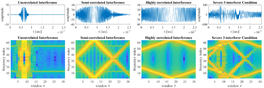
Fig. 2: Different types of interference with a single target in time domain (top) and time-frequency domain (bottom). From left to right, uncorrelated ($\gamma=0.5$), semi-correlated ($\gamma=1.5$), highly correlated interference ($\gamma=9$), and a case interfered by three types of interference.

3 Thresholding-based Interference Mitigation Algorithms

In this section, we introduce the core techniques of various thresholding based interference mitigation methods, namely TD-TH and TFD-TH. While TD-TH methods operate directly in the time domain to detect and eliminate interference, TFD-TH methods work in the time-frequency domain for the same purpose. A variety of time-frequency representations [20, 21] can be used, alongside various interference detectors such as constant false alarm rate (CFAR) [11, 12] or L-statistics[13, 16], to establish the threshold value $\beta$ for determining interference. However, the fundamental steps for thresholding are consistently applied across methods, as detailed in Algorithm 1 and 2. Note that the short-time Fourier transform (STFT) is presented here merely as an example. An in-depth discussion on the advantages and disadvantages of different time-frequency representations exceeds the scope of this paper.

Input: Received ADC Samples $\mathbf{Y}$

Output: $\mathbf{Y}_{c}$ after interference mitigation

1 $[M,N]=\mathbf{size}\{\mathbf{Y}\}$

2 for $i=1:M$  do

3      $\mathbf{x}=\mathbf{Y}(i,:)$

4       $\beta=\mathbf{IntfDetector}\{\mathbf{x}\}$

5       $\mathbf{x}(\mathbf{x}>\beta)=0$

6       $\mathbf{Y}_{c}(i,:)=\mathbf{x}$

7      

8 end for

Algorithm 1 Time Domain Thresholding (TD-TH)

Input: Received ADC Samples $\mathbf{Y}$

Output: $\mathbf{Y}_{c}$ after interference mitigation

1 $[M,N]=\mathbf{size}\{\mathbf{Y}\}$

2 for $i=1:M$  do

3      $\mathbf{x}=\mathbf{Y}(i,:)$

4       $\mathbf{X}=\mathbf{STFT}\{\mathbf{x}\}$

5       $[N_{r},N_{c}]=\mathbf{size}\{\mathbf{X}\}$

6      

7      for $k=1:N_{r}$ do

8             $\mathbf{z}=\mathbf{X}(k,:)$

9             $\beta=\mathbf{IntfDetector}\{\mathbf{z}\}$

10             $\mathbf{z}(\mathbf{z}>\beta)=0$

11             $\mathbf{X}_{c}(k,:)=\mathbf{z}$

12            

13       end for

14      $\mathbf{Y}_{c}(i,:)=\mathbf{STFT}^{-1}\{\mathbf{X}_{c}\}$

15      

16 end for

Algorithm 2 Time-Frequency Domain Thresholding (TFD-TH)

Comparing Algorithm 1 with Algorithm 2, it is evident that TD-TH methods typically have lower computational complexity than TFD-TH methods, primarily due to the additional STFT and inverse STFT operations in TFD-TH.

From (7) and Fig. 2, it is clear that in the presence of uncorrelated interference, only a minority of the ADC time samples are tainted by interference. This reduced impact is a direct result of the deramp mixing and the LPF in the receive chain. Therefore, after applying TD-TH, we can still employ the uncorrupted time samples for target range estimation. However, as the correlation between the interfering radar signal and the victim radar signal increases, more ADC time samples are corrupted according to (7) and Fig. 2. Specifically, in instances of highly correlated interference, the chirp slope of interference closely aligns with that of the victim radar. Consequently, the interference cannot be filtered by the LPF and the victim radar continually captures the interfering radar’s signal at its ADC output. This scenario compromises the efficacy of TD-TH. Furthermore, with increasing amounts of interference, another challenge emerges for TD-TH as shown in the severe 3-interferer condition presented in Fig. 2. Even if all interferences are uncorrelated interferences in the multiple-interferer example, their combined impact could corrupt the whole time samples. With each interference source corrupting a fraction of the ADC time samples, a point might be reached where all the samples are tainted, leaving none uncorrupted. This saturation further diminishes the performance of TD-TH. However, different interferences appear as distinct nonzero-slope linear features in the time-frequency domain, crossing the flat tones of target signals at distinct time and frequency components. Thus, in the time-frequency domain, the interference signals are distinctly recognizable and can be effectively isolated, ensuring that the target signals remain largely unaffected. Given the scenarios described, it becomes evident that the TFD-TH methods theoretically hold an advantage over the TD-TH approaches.

4 Numerical Results

Using the previously developed traffic scenario and automotive radar RFE simulator, radar signals with interference are generated to evaluate various interference mitigation algorithms. In this paper, we focused on two highway traffic scenarios with the targets being randomly positioned vehicles on the highway and guardrails along the edges of the highway. It is important to note that any vehicle target can potentially serve as a source of interference. The waveform configurations of interfering radars are randomly selected. Specific details are provided in Table 1, where Interference A, B, and C correspond to uncorrelated, semi-correlated, and highly correlated interference, as elaborated in section 2.3. In Scenario 1 (S1), uncorrelated interference predominates, accounting for $90\%$. In Scenario 2 (S2), on the other hand, highly correlated interference predominates.

Table 1: Highway Traffic Scenario

Traffic setting	Scenario 1 (S1)	Scenario 2 (S2)
Number of lanes	6	6
Type of targets	(vehicle, guardrail)	(vehicle, guardrail)
Number of targets	(34, 74)	(34, 74)
Interference A	90%	5%
Interference B	5%	5%
Interference C	5%	90%

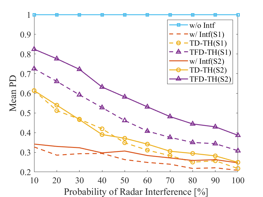
(a)

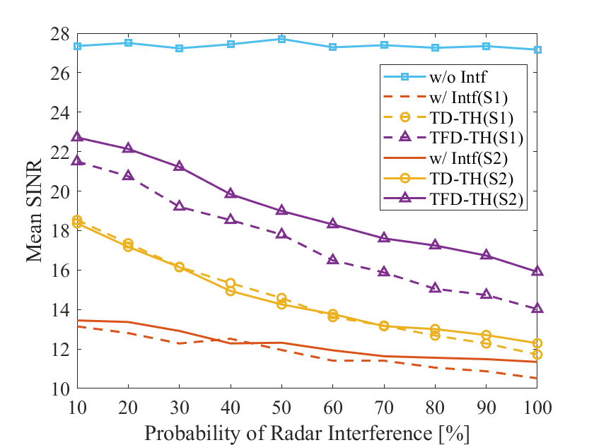
(b)

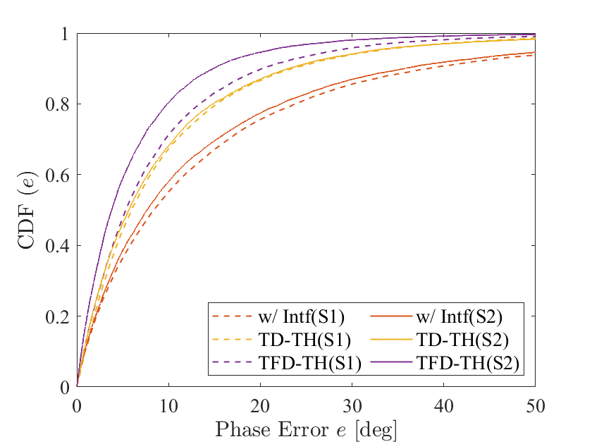
(c)

Fig. 3: Evaluation results of TD-TH and TFD-TH interference mitigation under interference scenario 1 (S1) and scenario 2 (S2): (a) PD, (b) SINR, and (c) phase error CDF.

To evaluate the performance of TD-TH and TFD-TH methods in S1 and S2, the PD, SINR, and phase error CDF are defined. Notably, some targets even cannot be detected by a typical detector under nominal conditions. Therefore, we refined the target cells in the RD map to focus on only detectable targets, chosen based on a nominal condition detector threshold, e.g., the threshold leading to a probability of false alarm equal to $0.001$. The PD is then derived from these detectable targets and the SINR is derived by computing the average power of these targets against the noise power present in the RD map. The phase of target bins in the RD map plays a crucial role in subsequent target angle estimation. To measure the impact of interference mitigation on this, we defined the phase error CDF:

$$\begin{split}\textrm{CDF}(e)=\textrm{Prob}\left\{\left\lvert\angle\mathbf{Y}(i,j)-\angle\mathbf{Y}_{c}(i,j)\right\rvert\leq e,\,\forall(i,j)\in\Theta\right\}\end{split}$$ (10)

Here, $\Theta$ represents the set of all target bins in the RD map and the phase error $\left\lvert\angle\mathbf{Y}(i,j)-\angle\mathbf{Y}_{c}(i,j)\right\rvert$ is scaled between $[0,180)$ degree.

In Fig. 3, we present the impact of interference mitigation techniques, TD-TH and TFD-TH, on PD, SINR, and phase error CDF as the probability of surrounding vehicles equipped with interfering radars, referred to as probability of radar interference, increases. When the probability of radar interference reaches $100\%$, all vehicles within the scenario act as interference sources. The curves in Fig. 3 represent how the evaluation metrics change with different probability of radar interference. Each point on these curves represents the average result from $100$ Monte Carlo experiments. Comparing the curves with and without interference, the presence of interference leads to a notable decline in SINR and a significant deterioration in the PD of the victim radar. The target phase also experiences significant degradation due to interference. Upon employing interference mitigation techniques, both TD-TH and TFD-TH enhance SINR. This leads to an improved PD and reduced phase error. Yet, as we vary the probabilities of radar interference, TFD-TH consistently outperforms TD-TH. The superiority of TFD-TH lies in its ability to preserve more target information within the time-frequency domain, as elaborated in section 3. TFD-TH shows superior performance in S2 compared to S1. This is due to the fact that, under uncorrelated interference conditions, the lower time resolution of the spectrogram makes TFD-TH’s outcomes more aligned with those of TD-TH. However, given the multiple interferences in S1, which falls into a kind of severe 3-interferer condition as illustrated in section 3, TFD-TH’s performance remains superior to TD-TH.

5 Conclusion

In this paper, we have evaluated the performance of TD-TH and TFD-TH in dense traffic scenarios with three different types of interference. Our numerical results highlight that TFD-TH consistently outperforms TD-TH as the number of interference increases. This performance gap widens notably when the correlation between the interfering radar signal and the victim radar signal intensifies. The key to TFD-TH’s superior performance lies in its ability to execute an accurate “surgical removal” of interference signals within the time-frequency domain. Interestingly, the time-frequency representation utilized by TFD-TH translates the signal into an image-like structure. This unique transformation unveils a promising avenue for leveraging data-driven techniques, such as deep learning, to remove interference in the time-frequency domain.

References

- [1] S. Sun, A. P. Petropulu, and H. V. Poor. MIMO radar for advanced driver-assistance systems and autonomous driving: Advantages and challenges. IEEE Signal Process. Mag., 37(4):98–117, 2020.
- [2] Shunqiao Sun and Yimin D Zhang. 4D automotive radar sensing for autonomous vehicles: A sparsity-oriented approach. IEEE Journal of Selected Topics in Signal Processing, 15(4):879–891, 2021.
- [3] Igal Bilik, Oren Longman, Shahar Villeval, and Joseph Tabrikian. The rise of radar for autonomous vehicles: Signal processing solutions and future research directions. IEEE Signal Processing Magazine, 36(5):20–31, 2019.
- [4] Jun Li, Ryan Wu, I-Tai Lu, and Dongyin Ren. Bayesian linear regression with cauchy prior and its application in sparse mimo radar. IEEE Transactions on Aerospace and Electronic Systems, 59(6):9576–9597, 2023.
- [5] S. Alland, W. Stark, M. Ali, and A. Hedge. Interference in automotive radar systems: Characteristics, mitigation techniques, and future research. IEEE Signal Process. Mag., 36(5):45–59, 2019.
- [6] Jonathan Bechter, Fabian Roos, Mahfuzur Rahman, and Christian Waldschmidt. Automotive radar interference mitigation using a sparse sampling approach. In 2017 European Radar Conference (EURAD), pages 90–93. IEEE, 2017.
- [7] Christoph Fischer. Untersuchungen zum interferenzverhalten automobiler radarsensorik. Cuvillier Verlag, 2016.
- [8] Farrokh Marvasti, Masoume Azghani, P Imani, P Pakrouh, Seyed Javad Heydari, Azarang Golmohammadi, A Kazerouni, and MM Khalili. Sparse signal processing using iterative method with adaptive thresholding (IMAT). In 2012 19th International Conference on Telecommunications (ICT), pages 1–6. IEEE, 2012.
- [9] B-E Tullsson. Topics in FMCW radar disturbance suppression. 1997.
- [10] Mate Toth, Paul Meissner, Alexander Melzer, and Klaus Witrisal. Performance comparison of mutual automotive radar interference mitigation algorithms. In 2019 IEEE Radar Conference (RadarConf), pages 1–6. IEEE, 2019.
- [11] Francesco Laghezza, Feike Jansen, and Jeroen Overdevest. Enhanced interference detection method in automotive FMCW radar systems. In 2019 20th International Radar Symposium (IRS), pages 1–7, 2019.
- [12] Jianping Wang. CFAR-based interference mitigation for FMCW automotive radar systems. IEEE Transactions on Intelligent Transportation Systems, 23(8):12229–12238, 2021.
- [13] Ryan Haoyun Wu, Jun Li, Maik Brett, and Michael Andreas Staudenmaier. Radar communication with interference suppression, November 3 2022. US Patent App. 17/245,613.
- [14] Ryan Haoyun Wu, Jun Li, and Christian Tuschen. Radar communication with interference suppression, December 7 2023. US Patent App. 18/453,931.
- [15] Sefa Tanis. Automotive radar sensors and congested radio spectrum: An urban electronic battlefield? Analog Dialogue, 52(3):1–5, 2018.
- [16] Robert Muja, Andrei Anghel, Remus Cacoveanu, and Silviu Ciochina. Interference mitigation in FMCW automotive radars using the short-time fourier transform and l-statistics. In 2022 IEEE Radar Conference (RadarConf22), pages 1–6. IEEE, 2022.
- [17] Sian Jin, Pu Wang, Petros Boufounos, Philip V Orlik, Ryuhei Takahashi, and Sumit Roy. Spatial-domain interference mitigation for slow-time MIMO-FMCW automotive radar. In 2022 IEEE 12th Sensor Array and Multichannel Signal Processing Workshop (SAM), pages 311–315. IEEE, 2022.
- [18] Faruk Uysal and Sasanka Sanka. Mitigation of automotive radar interference. In 2018 IEEE Radar Conference (RadarConf18), pages 0405–0410. IEEE, 2018.
- [19] Dilge Terbas, Francesco Laghezza, Feike Jansen, Alessio Filippi, and Jeroen Overdevest. Radar to radar interference in common traffic scenarios. In 2019 16th European Radar Conference (EuRAD), pages 177–180. IEEE, 2019.
- [20] Boualem Boashash. Time-frequency signal analysis and processing: a comprehensive reference. Academic press, 2015.
- [21] Ivan W Selesnick. Short-time fourier transform and its inverse. Signal, 10(1):2, 2009.