Particle detection performance and Geant4 simulation with low-cost CMOS technology

Abstract

We analyze the performance of an Omnivision OV5647 CMOS image sensor (5 Mp) for measuring the radiation emitted from Sr90 and Cs137 sources. Our experimental arrangement includes a Raspberry Pi 3 mini-computer for data taking, processed with Python and OpenCV libraries. We specify the camera settings to be sensitive to detecting electrons and photons. We also implement a detailed Geant4 simulation of the CMOS sensor and the radioactive sources. This simulation connects the deposited energy in the pixel matrix by the electrons and photons from the radioactive sources and the ADC counts. Our measurements are expressed through the cluster size, the maximum ADC signal per cluster, and the variation of the clusters with different distances. We find a good agreement between the data and the Geant4 simulation for all these observables. Furthermore, we can reproduce the correlation between the cluster size and the maximum ADC per cluster.

[inst1]organization=Sección Física, Departamento de Ciencias, Pontificia Universidad Católica del Perú,addressline=Av. Universitaria 1801, city=Lima, postcode=15088, country=Perú

[inst2]organization=UNSAAC,addressline=Av. De la Cultura, 733,, city=Cusco, postcode=8000, country=Perú

1 Introduction

Imaging sensors based on metal oxide semiconductors (CMOS), designed to take photographs, have been widely used to detect particles such as gamma rays, electrons, alphas, etc [1, 2, 3, 4]. One low-cost commercial CMOS sensor that has been used for this purpose is the 5 Mp OmniVision OV5647 camera, which has shown good results in particle detection, such as discriminating between alpha and non-alpha particles by identifying and extracting ionization events [3] and photon imaging using fluorescence X-rays and gamma rays [4, 5].

In this work, we define a simple experimental setup to detect electrons and photons from radioactive sources using the OV5647 sensor inside a dark box. The setup includes a Raspberry Pi 3b for data taking and precisely configuring the sensor settings with Picamera libraries, for making stable and sensitive measurements.

To reproduce the data, we implement a detailed simulation of the geometry and materials of the OV5647 sensor with Geant4 and also simulate its irradiation with radioactive sources (Sr90 and Cs137). We transform deposited energy to ADC counts and then identify clusters of pixels signaling particle events.

This paper is divided as follows: in section 2 we describe the experimental setup, the characteristics of the OV5647 CMOS sensor, and the radioactive sources. Section 3 describes data collection and processing with the help of the Picamera libraries. Section 4 explains how we perform the simulation of the sensor and radioactive sources in Geant4. Section 5 describes data processing with the help of OpenCV libraries, the methods used to reduce background noise, and the search for clusters representing particle tracks in the images. In section 6 we show the results of comparing the simulation with the experimental data for different parameters related to the number of ADC counts and clusters. We also study the behavior of the clusters with distance and the possibility of differentiating between radioactive sources. Finally, in section 7 we give our conclusions.

2 Experimental setup

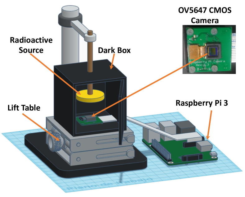
To test the CMOS sensor for particle detection, we designed the experimental configuration shown in Fig.1 (devices not to scale). In the lower part, we placed a lift table, which moves the sensor along the $z$ axis and has a resolution of $100\pm 50$ $\mu$m, allowing us to control the distance between it and the radioactive source.

On the lift table, we put an aluminum dark box (68.87$\pm 0.01$ mm high with a squared base of side 88.06$\pm 0.01$ mm), black painted and sealed with black PVC insulation tape to ensure it is light-tight. Inside the dark box, we placed a radioactive source fixed to a support inside the box. The detector (OmniVision OV5647 CMOS sensor [6]) is placed at the base of the dark box.

To capture the frames with the OV5647 camera we used a Raspberry Pi 3b (i.e. a small, low-cost single-board computer [7, 8] ). To avoid light leakage to a minimum we connect the OV5647 camera via a flexible cable to the Raspberry Pi 3b.

Figure 1: Experimental setup to capture 10-bit images (the CMOS sensor, the radioactive source, and the Raspberry Pi 3 are to scale, while the other devices are not).

2.1 OmniVision OV5647 Sensor

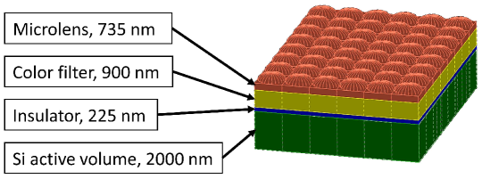
The OmniVision OV5647 sensor (5 Mp) is a low-cost camera module that can be used along with a Raspberry Pi. It has a resolution of 2592 $\times$ 1944 pixels, with a pixel pitch of 1.4 $\times$ 1.4 $\mu$m² and a 3.67 $\times$ 2.73 mm² active area [6]. The cross-section of the OV564 CMOS sensor, as measured in [9, 4], shows the following layers and their thickness from top to bottom: microlenses for each pixel made from PDMS (SiOC₂H₆) (0.735 $\mu$m), the photoresist (C₁₀H₆N₂O) color filter to enable RGB imaging (0.9 $\mu$m), a thin insulator layer of SiO₂ (0.225 $\mu$m) and the sensitive Si detection volume (2 $\mu$m).

The CMOS sensor pixels can detect photons and electrons. In the case of photons, the photoelectric effect converts them into electron-hole pairs. Electrons ionize the medium also creating electron-hole pairs, which are later collected by the electronics. The energy used to generate an electron-hole pair in Si is on average 3.6 eV [10, 11, 3, 12, 13]), for photons, as well as, approximately, for electrons. The maximum possible electrical load is called "Full Well Capacity", (FWC). Above the FWC the pixel will saturate and the accumulated charge will be equal to a maximum value [3, 14, 15]. The FWC of the OV5647 sensor pixels is approximately 4300 electrons according to the datasheet [6].

To get the source as close to the sensor as possible, the optical lens of the OmniVision OV5647 camera was removed, exposing the pixel sensor as shown in Fig. 1.

2.2 Radioactive sources

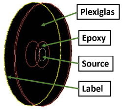
The radioactive sources that were used are Sr90 and Cs137 from Spectrum Techniques in the form of cylindrical tablets. Inside an epoxy cylinder of 0.25" in diameter with a height of 0.11" is the radioactive source. This disk, as shown in Fig. 2, is encased in a plexiglass cylinder of 1.010" diameter with a height of 0.125" [16].

Figure 2: Radioactive source geometry provided by the manufacturer [16].

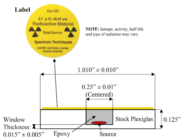
The Sr90 and Cs137 sources decay almost entirely by emission of $\beta^{-}$ particles (electrons). The Sr90 source emits electrons with a maximum energy of 0.546 MeV and the resulting Y90 isotopes also decay into electrons with a maximum energy of 2.28 MeV. Thus, Sr90 is technically a pure electron source, since gamma photon emission is negligible ([17], [18]). The characteristics provided by the manufacturer show that the Sr90 source was produced in July 2015 with an activity of 0.1 $\mu$Ci and a half-life of 28.8 years. With these data, we calculate the activity during data taking (i.e. October 2023) to be 3028 Bq.

The electron emission in Cs137 decay is about 94.6% with an energy of 0.514 MeV, producing Ba-137m, which emits a 0.662 MeV photon. Thus, Cs137 is a mixed source of electrons and photons [17], [18]. The characteristics provided by the manufacturer show that the Cs137 source was produced in June 2015 with an activity of 0.25 $\mu$Ci and a half-life of 30.1 years. With these data, we calculate the activity during data taking (i.e. October 2023) to be 0.21 $\mu$Ci.

3 Data acquisition

To record the data with our experimental setup we use a Raspberry Pi3 and Picamera libraries [19]. The latter allows us to configure the parameters of the OV5647 sensor. The regular use of the OV5647 is to take photographs, with that purpose various camera settings can change according to light conditions. Therefore, to ensure stability in the data acquisition we require to fix the following settings:

• Shutter speed = 0.5 seconds (i.e. the exposure time with which each frame will be taken). This time is enough to capture $\mathcal{O}(10^{3})$ radioactive decay from the selected sources.

• Image resolution = $2592\times 1944$ pixels (5 Mp), which is the maximum resolution.

• Analog gain = 8. This gives the maximum stable response of the camera without image distortion.

• Digital gain = 1. This is an artificial gain done by software set to its minimum value.

• White balance = 1. This value is equivalent to no color correction since we are not looking at visible light.

For capturing images we use the 10-bit Bayer format for the ADC counts. This format is defined by three color matrices (RGB) distributed in the CMOS sensor, so that 25% of the pixels are red, 50% green, and 25% blue [19]. Since we are interested only in the intensity of each pixel and not its color, we add these three partial matrices to obtain a full matrix with the intensities in ADC values and save them in Python ’npz’ format.

To obtain the background we captured 1000 frames, equivalent to 500 seconds of actual exposure time, with the OV5647 inside the dark box without a radioactive source. The processing of each frame with the Raspberry Pi including the matrix conversion and the data saving is approximately 11.5 seconds per frame, adding to a total of about 3 hours and 11 minutes of data taking.

Then, a radioactive source (Sr90 and Cs137, respectively) is placed on top of the OV5647 sensor at a distance of 0 mm between the source and the detector. In this configuration, the radioactive source with a circular area of 7.92 mm² illuminates approximately 74% of the rectangular surface of the 10.02 mm² pixel sensor. The same amount of frames and duration were taken in the background measurement.

Additionally, with the help of the lift table (Fig.1), the detector is moved away from the radioactive source, which is fixed by the support until there is a separation of 2 mm between them, and we take 100 frames each 0.5 seconds of data every 2 mm. This procedure is repeated every 2 mm until an 18 mm separation between the source and the detector is reached. The latter has been implemented to test the inverse square distance law based only on the Sr90 source measurements.

4 Geant4 Simulation

We used a detailed Geant4 [20] simulation of the OmniVision OV5647 CMOS sensor to reproduce the experimental data. For this, the dimensions and materials of the CMOS sensor mentioned in section 2.1 were used to define its geometry and composition. The geometry of the radioactive sources (i.e., Sr90 and Cs137) was simulated according to the specifications provided by the manufacturer, mentioned in section 2.2. This paper’s simulation code and scripts can be found in the supplementary material [21].

A fragment of the simulated CMOS sensor geometry and the simulated radioactive source geometry are shown in Fig. 3. The dark box was not simulated since it is large enough compared to the sensor, not affecting the measurement. Also, the distance between the source and the sensor is smaller than the dark box size.

Figure 3: Simulated geometry of a fragment (6$\times$8 pixels) of the CMOS sensor (left) and the radioactive source (right).

The number of simulated events is equivalent to the number of disintegrations for a given time, i.e., the activity of the radioactive source at the measurement time. The Sr90 source had an activity corresponding to 1514 events every 0.5 seconds (i.e., the exposure time of each frame) at the time of the measurement on October 2023. The Cs137 activity corresponds to 3811 events per 0.5 seconds.

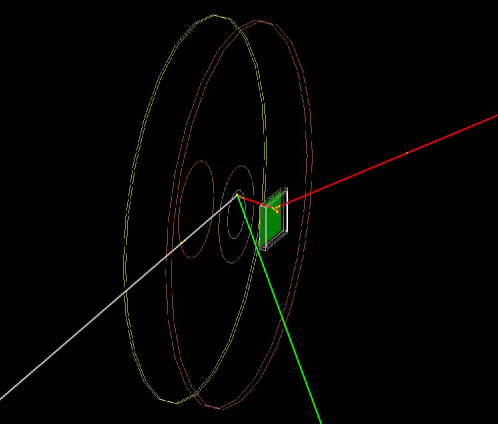
Fig. 4 shows an example of 1 event of the Geant4 simulation of the particles emitted by a Cs137 radioactive source to the CMOS sensor, where the track left by the electron is red, the electron antineutrino track is white, and the photon is green.

Figure 4: Geant4 simulation of the particles emitted by a Cs137 source. Red lines represent electrons, the white lines are the electron antineutrino and the green lines are photons.

The simulation in Geant4 gives us the energy deposited in the pixel matrix. We convert this deposited energy into electron-hole pairs in Si, using the aforementioned factor of 3.6 eV per pair. From the number of pairs, we extrapolate the number of electrons used in the rest of the simulation chain.

After transforming the deposited energy per pixel into a number of electrons, we convert the number of electrons of each pixel into ADC counts. As we have pointed out, the maximum number of electrons before saturation is 4300 electrons, corresponding to the FWC. The minimum is 5 electrons, equivalent to one ADC count (obtained from dividing 4300 electrons over 1023 ADC counts).

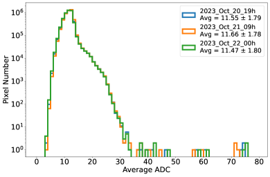
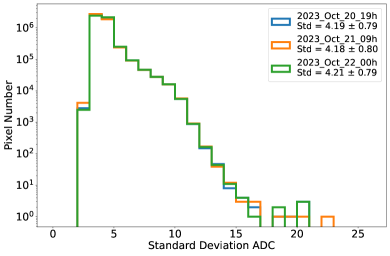
Finally, we performed background measurements for three days at different times, showing a variation of 0.04% to 0.08% of active pixels, the average ADC value was between 11.5 and 11.7 with an error of 1.8, and their standard deviation was 4.2 $\pm$ 0.8. This variation is minimal, so we can consider that the background is stable over time. Fig. 5, shows the distribution of the average and standard deviation of the data taken for the background noise.

Figure 5: Distribution of the average (left) and standard deviation (right) for 1000 frames of the background noise of 3 datasets on different days.

5 Data analysis

The electronics produce a non-negligible noise during the pixel readout, especially when working with low signals. This noise causes, in our case, that 99.48 % of the pixels have a signal detected in the experimental data.

To reduce this background noise in the experimental data a two steps procedure was applied: (1) the average ADC for each pixel from the background data (11.5 ADC on average) was subtracted from the experimental measurements, reducing it to 43.6% of active pixels. (2) After the subtraction, a five standard deviations ADC threshold for each pixel from the background (5$\sigma$=21.1 ADC on average) was applied, reducing it to 0.0047% of active pixels (i.e. 236474 active pixels). From now on, the aforementioned process, that we call as Standard Noise Reduction (SNR), will be applied by default to all the data presented in our work, unless otherwise specified.

Assuming that this background noise is stable and evenly distributed in the pixel matrix, this procedure should reduce most noise. This method does not affect signal events with large ADC values. However, this is not the case for low ADC signals. Nevertheless, it is not possible to distinguish between one pixel with a low ADC coming from background from a similar one from signal.

Using the OpenCV (Open Computer Vision) libraries [22], clusters (i.e., a pixel or groups of pixels with a signal different than zero and adjacent to each other) are searched for in all frames. In our analysis, we will study three observables: the ADC distribution, the cluster size, and the maximum ADC per cluster.

When analyzing the cluster size (defined by its number of pixels), we found that the background noise is mostly present in the smallest clusters of 5 pixels at most, and we cannot differentiate between the signal and the background for clusters of similar size. Therefore, on top of the SNR procedure, we make a cut on the cluster size discarding clusters composed by less than or equal to 3 pixels, removing 97% of the remaining background clusters. Using this filtered sample, we analyze the maximum ADC per cluster. The application of this cut will enable us to compare this reduced data sample, nearly devoid of background clusters, with the Geant4-simulated signal that also underwent the 3-pixel cut.

The result of our statistical analysis will be shown in terms of the reduced $\chi^{2}_{\nu}$ defined as $\chi^{2}/\nu$ where $\nu$ is the number of degrees of freedom.

6 Results

We present the results of the comparison between our experimental data and the Geant4-simulation of the camera, when it is irradiated by a radioactive source. As we already mentioned, this analysis will be performed for three observables: the ADC distribution, the cluster size, and the maximum ADC per cluster, considering as sources: Sr90 and Cs137. Furthermore, by moving the radioactive sources to various distances, we will investigate the square inverse distance law of irradiation.

In general, the experimental data show the statistical uncertainty, while the simulation uncertainty is the systematic one that comes from the uncertainty in the source activity, which is assumed as 20% error on the source activity, according to the datasheet [16]. As we anticipated, the experimental data displayed in all the plots has already been filtered by our SNR procedure.

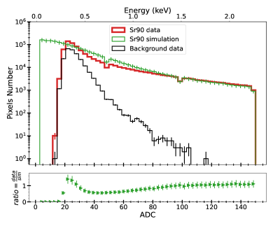
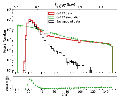
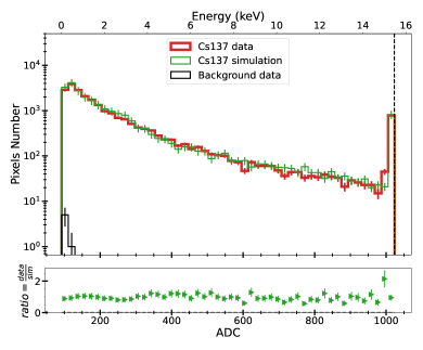
Fig. 6, compares the ADC distributions at the pixel level for all cluster sizes for the experimental data and its corresponding simulation, for both Sr90 and Cs137. It is important to note that the signal saturation is reached at 1023 ADC, equivalent to 15.48 keV of deposited energy. The background noise only attains up to 115 ADC.

In the plots at the top, the experimental data is presented after applying the SNR procedure. In both plots (left and right), the background is noticeable and located at the first bins. In the case of Sr90, the average number of active pixels for the experimental data, after applying the SNR procedure, is 0.016%, while for the Geant4 signal simulation, it is 0.035%. Analogously, for Cs137, the average number of active pixels for the experimental data is 0.008%, and for the simulation, 0.007%, which is a lower number than for Sr90, even if the activity of the Cs137 source is higher. The electrons of the Sr90 produce more active pixels than the electrons from Cs137 because the former can reach higher energy, being that there are fewer electrons from Cs137 that can deposit energy in the detector in comparison with the electrons coming from Sr90. The latter is clearly illustrated in the plots at the bottom of Figs. 6, in which we are zooming in the region up to 150 ADC, where the ADC distribution for Sr90 is higher than for Cs137.

Figure 6: ADC number distribution at 0 mm between sensor and source, for 500 s exposure time for the experimental and simulated data for Sr90 (top left) and Cs 137 (top right), the experimental data applying the SNR procedure and comparing with pure simulation, the vertical dotted line shows the saturation level of the CMOS sensor at 1023 ADC equivalent to 15.48 keV. At the bottom a zoom of the same distributions for the region between 1 and 150 ADC for Sr90 (bottom left) and Cs137 (bottom right).

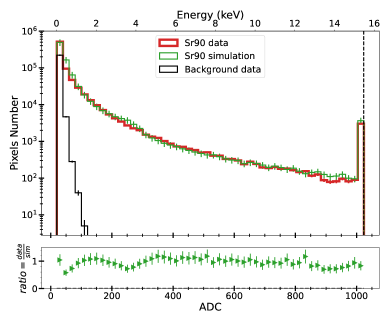
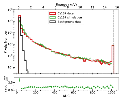
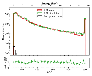
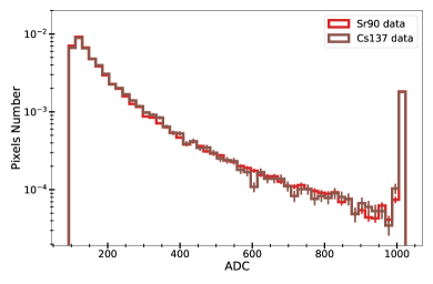
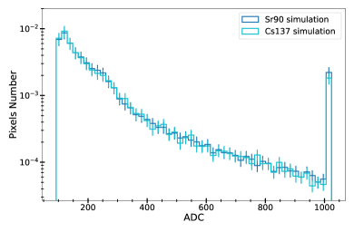
To remove the background at the first bins, as shown in Figs 6, we cut the events below 100 ADC. After this cut, the background left is minimal, and the Sr90 average number of active pixels is reduced to 0.002%, while for Cs137 reaches 0.0005%, getting for both radioactive sources an excellent agreement in terms of the number of active pixels between the experimental data and the simulation. In Fig. 7 we display the ADC distribution after applying the aforementioned cut. Here, we can see a very good agreement between the ADC distributions from the experimental data and the simulation for both sources. This is confirmed by the reduced chi-square test ($\chi^{2}_{\nu}$) for these ADC distributions, where we obtain a $\chi^{2}_{\nu}$ for Sr90 of 0.55, while for Cs137 is 0.82.

Figure 7: ADC number distribution for the experimental and simulated data with a cut to remove values less than or equal to 100 ADC for Sr90 (left) and Cs 137 (right), the experimental data applying the SNR procedure and comparing with pure simulation at 0 mm between sensor and source, for 500 s exposure time. The vertical dotted line shows the saturation level of the CMOS sensor at 1023 ADC equivalent to 15.48 keV

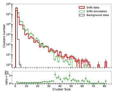
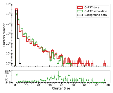
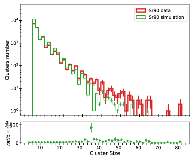
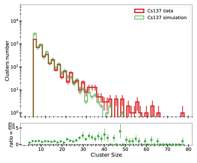
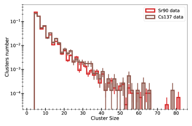
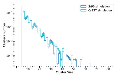
The top panels in Fig. 8 show the cluster size distribution for experimental data and background after the SNR procedure is applied for both sources. The cluster size distribution shows that the background is present up to the five-pixel cluster, where most of them are located below the three-pixel cluster size. Therefore, on top of the SNR procedure, we apply two cuts: one is for removing clusters with less and equal to a three-pixel cluster size. The other cut removes clusters that have a maximum value of ADC, considering each of its pixels is less than 100 ADC. The application of all these cuts is shown at the bottom panels in Fig. 8. Here, it can be observed the improvement of the agreement between the cluster size distribution for data and simulation after the cut is applied. Considering these distributions, the $\chi^{2}_{\nu}$ value for Sr90 is 2.24, and for Cs137 is 1.26. These values indicate that there is a slight discrepancy between the experimental data and the simulation.

Figure 8: Cluster size distribution for the experimental and simulated data for Sr90 (top left) and Cs 137 (top right), the experimental data applying the SNR procedure and comparing with pure simulation. At the bottom are the same distributions removing the cluster size less than or equal to a three-pixels, and removing clusters that have a maximum value of ADC, considering each of its pixels is less than 100 ADC for Sr90 (bottom left) and Cs 137 (bottom right) at 0mm between sensor and source for 500 s exposure time.

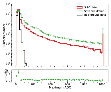
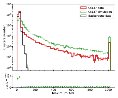
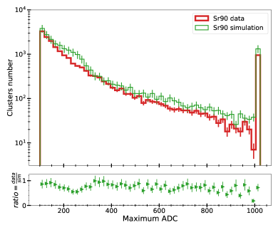
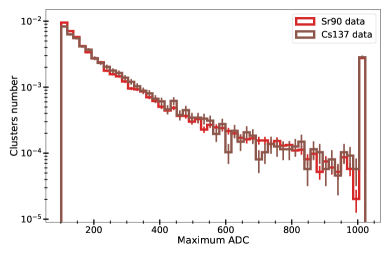
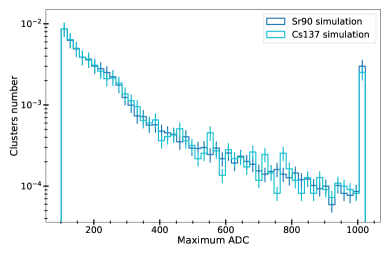
Another parameter we analyze is the distribution of the maximum ADC signal per cluster for the same data set as before, shown in Fig. 9. At the top panels, we have the maximum ADC signal per cluster distribution after applying the SNR procedure. In this case, the simulated data distribution is higher than the experimental data along the entire range of maximum ADC signal per cluster. Also, we appreciate the signal saturation at a maximum of 1023 ADC. At the bottom panels and on top of the SNR procedure, we apply the same two cuts as in the case of the cluster size distributions. As a result, for these maximum ADC signal per cluster distributions, the $\chi^{2}_{\nu}$ value for Sr90 is 2.10, and for Cs137, it is 1.96.

Figure 9: Maximum ADC signal per cluster distribution for the experimental and simulated data for Sr90 (top left) and Cs 137 (top right), the experimental data applying the SNR procedure and comparing with pure simulation. At the bottom are the same distributions removing the cluster size less than or equal to a three-pixels, and removing clusters that have a maximum value of ADC, considering each of its pixels is less than 100 ADC for Sr90 (bottom left) and Cs 137 (bottom right) at 0 mm between sensor and source for 500 s exposure time.

To give the reader a summarized perspective of our results, we present in Table 1, the $\chi^{2}_{\nu}$ for the three observables we study: the ADC distribution, the cluster size, and the maximum ADC per cluster distributions. The SNR filter has been applied to the experimental data for all of these distributions. As mentioned before, an extra cut rejecting pixels with less or equal to 100 ADC units has been applied for the ADC distributions in the data and the simulation. For the cluster size and the maximum ADC per cluster distributions, as mentioned already, we impose two cuts to the simulation and data, these are: one removes cluster size less than or equal to three-pixel size, and the other is to remove clusters that have a maximum value of ADC, considering each of its pixels is less than 100 ADC. As we can see the best agreement we obtained is for the ADC distributions, being very reasonable the ones we got for the cluster size and the maximum ADC per cluster distributions, considering the limitations we face. In that sense, it is crucial to remark that the design characteristics of the OV5647 CMOS are aimed at optimizing a photographic image by artificially amplifying the intensities and other parameters of the pixels. The latter is out of our control since it cannot be handled via standard software.

	$\chi^{2}_{\nu}$
Source	Sr90	Cs137
ADC number (cut >100 ADC)	0.55	0.82
Cluster Size	2.24	1.26
Maximum cluster ADC	2.10	1.96

Table 1: The $\chi^{2}_{\nu}$ tests with 50 bins when comparing the experimental data applying the SNR procedure with simulation. For the ADC distributions with a cut of 100 ADC, and for the distributions related to the number of clusters (i.e., size, and maximum ADC signal) with two cuts to remove the cluster size less than or equal to a three-pixels, and remove clusters that have a maximum value of ADC for Sr90 and Cs137 at 0 mm distance between sensor and source for 500 s exposure time.

We also looked for correlations between variables in 2D histograms of the cluster size vs maximum ADC signal per cluster, for Sr90 and Cs137 at 0 mm distance between source and detector for the data and the simulation. Fig 10 show these distributions.

Figure 10: Cluster size versus maximum ADC signal per cluster for the experimental and simulated data for Sr90 (left) and Cs 137 (right), the experimental data applying the SNR procedure and comparing with simulation, removing the cluster size less than or equal to a three-pixels, and removing clusters that have a maximum value of ADC, considering each of its pixels is less than 100 ADC at 0 mm between sensor and source for 500 s exposure time.

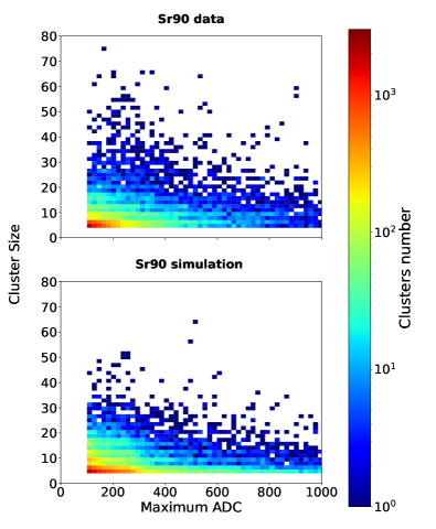
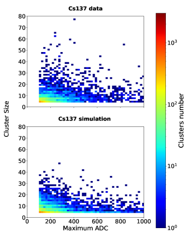
In Fig. 10, we can observe that the simulated data for these distributions are close to the experimental data for both Sr90 and Cs137. Due to the background noise, the experimental data show more scattered clusters above 30 pixels than in the simulation. The $\chi^{2}_{\nu}$ for these distributions is 1.68 for Sr90 and 1.63 for Cs137, showing a good agreement.

In addition, to verify the inverse square distance law behavior of the Sr90 radioactive source we performed measurements every 2 mm from 0 to 18 mm between the source-detector distance, taking 100 frames per each distance selected. In Fig. 11 we show the average number of clusters at different distances ($z$) for both the experimental data with noise reduction SNR procedure and the simulation and their respective fits to $a/(z+b)^{2}$ (i.e. the inverse square of the distance, where $a$ and $b$ are free parameters)

Figure 11: Average cluster number, as a function of distance ($z$) for the Sr90 source. The experimental data applying the SNR procedure is in red and the pure simulation without cuts is in green. Both data and simulation are fitted to the inverse square function $y=a/(z+b)^{2}$.

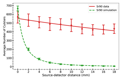
The simulation shows the expected behavior with distance, but the experimental data does not. This is because there is a large background noise of a few pixel clusters, as mentioned previously, due to the physical and acquisition software characteristics of the CMOS sensor. As the source moves away from the sensor, the background noise remains constant while the signal clusters diminish, showing a more linear behavior for the experimental data.

To show the expected behavior of the signal with distance, we apply to the experimental data the cut of cluster less than or equal to three pixels to remove the background and no cut to the simulation. If we apply the same cut to the simulation, it would have a larger effect for distances greater than 0 mm, producing an abrupt change, reducing the sample in average to less than 1 cluster after 4 mm.

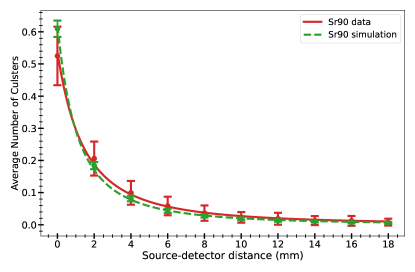
To better appreciate the behavior with the souce-detector distance we normalize both distributions since the cut to the experimental data lowers the cluster count. Fig. 12 shows that these adjustments follow the inverse square of the distance. The parameters obtained for these fits are $a=4.47\pm 0.27$, $b=2.89\pm 0.11$ for the experimental data, and for the simulation $a=2.99\pm 0.15$, $b=2.20\pm 0.07$, with a $\chi^{2}_{\nu}$ of 0.04 and 0.46 for the fit of experimental and simulated data, respectively. This demonstrates the expected behavior for the source-detector distance for both experimental data and the simulation.

Figure 12: Average cluster number, as a function of distance ($z$) for the Sr90 source. The experimental data applying the SNR procedure and a cut in a cluster less than or equal to three pixels is in red and the pure simulation is in green. Both data are fitted to the inverse square function $y=a/(z+b)^{2}$.

To know if the Sr90 and Cs137 sources can be distinguished, we compare the distributions discussed above at the 0-mm distance. Then, we normalize the histograms to avoid differences in the activities of the sources. Fig. 13, 14, and 15 show the normalized distributions at the pixel and cluster level after applying the cuts. The $\chi^{2}_{\nu}$ for the comparison between the two sources in the experiment and the simulation is shown in Table 2. The average $\chi^{2}_{\nu}$ for the experimental data is 1.52, and for the simulation, it is 2.25. Thus, it is impossible to distinguish between these two radioactive sources for the camera capabilities.

	$\chi^{2}_{\nu}$
Source	Experiment	Simulation
ADC number (cut >100 ADC)	1.46	0.17
Cluster Size	1.79	5.87
Maximum cluster ADC	1.32	0.71

Table 2: The $\chi^{2}_{\nu}$ test with 50 bins when comparing the experimental data applying the SNR procedure, and simulation of Sr90 with Cs137 for the normalized ADC distributions with a cut of 100 ADC and the normalized distributions related to the number of clusters (i.e. size, and maximum ADC signal) with two cuts to remove the cluster size less than or equal to a three-pixels, and remove clusters that have a maximum value of ADC signal per cluster 0 mm distance between source and detector for 500 s exposure time.

Figure 13: Normalized ADC number distribution comparing the sources of Sr90 and Cs137 for the experimental data (left) and the simulation (right), experimental data applying the SNR procedure comparing with simulation applying a cut to both to remove values less than or equal to 100 ADC to both the experimental data and the simulation at 0mm between sensor and source, for 500 s exposure time.

Figure 14: Normalized cluster size distribution comparing the sources of Sr90 and Cs137 for the experimental data (left) and the simulation (right), experimental data applying the SNR procedure comparing with simulation, removing the cluster size less than or equal to a three-pixels, and removing clusters that have a maximum value of ADC, considering each of its pixels is less than 100 ADC at 0mm between sensor and source for 500 s exposure time.

Figure 15: Normalized maximum ADC signal per cluster distribution comparing the sources of Sr90 and Cs137 for the experimental data (left) and the simulation (right), experimental data applying the SNR procedure comparing with simulation, removing the cluster size less than or equal to a three-pixels, and removing clusters that have a maximum value of ADC, considering each of its pixels is less than 100 ADC at 0mm between sensor and source for 500 s exposure time

7 Conclusions

In this work, we implement a system for the data acquisition of the OmniVision OV5647 CMOS sensor with the help of a Raspberry Pi. We give precise information about the settings needed for the camera to take stable and sensitive frames for detecting particles. To reduce the experimental noise we subtract the average ADC value per pixel and apply a 5 sigma ADC threshold per pixel obtaining a reduction of 99.995% of active pixels.

We conclude from the $\chi^{2}_{\nu}$ of the analyzed distributions, for Sr90 and Cs137, that the simulation is in good agreement with the experimental data, considering the characteristics of the CMOS sensor. It is possible to carry out simulations of commercial sensors such as CMOS cameras if their physical specifications are precisely described. In addition, we can reproduce the correlation between variables (e.g. cluster size vs. maximum ADC per cluster) with a $\chi^{2}_{\nu}$ that shows good agreement for Sr90 and Cs137.

We analyzed how the detected source emission varies with the distance when the background noise is completely removed, finding that both the experimental data and the simulation follow an inverse square distribution, as expected.

When comparing the experimental data for the sources of Sr90 and Cs137 using their different parameters, we found that it is not possible with this experimental method to distinguish between the radioactive sources, nor using pure simulation.

A further step would be to identify the type of detected particles by the shape of the clusters and compare them between data and simulation.

References

- [1] M. Pérez, et al., Particle detection and classification using commercial off the shelf cmos image sensors, NIM-A 827 (2016) 171–180. doi:10.1016/j.nima.2016.04.072.
- [2] M. Pérez, et al., Commercial CMOS pixel array for beta and gamma radiation particle counting, in: 2015 EAMTA, 2015, pp. 11–16. doi:10.1109/EAMTA.2015.7237371.
- [3] C. L. Galimberti, et al., A low cost environmental ionizing radiation detector based on COTS CMOS image sensors, in: IEEE ARGENCON, 2018, pp. 1–6. doi:10.1109/ARGENCON.2018.8645967.
- [4] J. Lipovetzky, et al., Multi-spectral X-ray transmission imaging using a BSI CMOS image sensor, Radiation Physics and Chemistry 167 (2020) 108244. doi:10.1016/j.radphyschem.2019.03.048.
- [5] J. Lipovetzky, et al., Multi-spectral X-ray transmission imaging using a BSI CMOS image sensor, Radiation Physics and Chemistry 167 (2020) 108244. doi:10.1016/j.radphyschem.2019.03.048.
- [6] Datasheets OV5647 camera module, https://gzhls.at/blob/ldb/b/3/1/9/4b75ea96beae68ee985c5bc3ca988cf4f29a.pdf, accessed: 2024-02-20 (2022).
- [7] Raspberry Pi 3B, https://datasheets.raspberrypi.com/rpi3/raspberry-pi-3-b-plus-product-brief.pdf, accessed: 2024-02-20 (2023).
- [8] Raspberry Pi, https://www.raspberrypi.org/, accessed: 2024-02-20 (2020).
- [9] A. Bessia, et al., X-ray micrographic imaging system based on COTS CMOS sensors, International Journal of Circuit Theory and Applications 46 (10) (2018) 1848–1857. doi:10.1002/cta.2502.
- [10] J. Fang, et al., Understanding the average electron–hole pair-creation energy in silicon and germanium based on full-band Monte Carlo simulations, IEEE Transactions on Nuclear Science 66 (1) (2019) 444–451. doi:10.1109/TNS.2018.2879593.
- [11] M. Brigida, et al., A new Monte Carlo code for full simulation of silicon strip detectors, NIM-A 533 (3) (2004) 322–343. doi:10.1016/j.nima.2004.05.127.
- [12] F. Scholze, et al., Determination of the electron-hole pair creation energy for semiconductors from the spectral responsivity of photodiodes, NIM-A 439 (2000) 208–215. doi:10.1016/S0168-9002(99)00937-7.
- [13] P. Lechner, R. Hartmann, H. Soltau, L. Strüder, Pair creation energy and Fano factor of silicon in the energy range of soft X-rays, NIM-A 377 (2) (1996) 206–208. doi:10.1016/0168-9002(96)00213-6.
- [14] D. W. Lane, X-ray imaging and spectroscopy using low cost COTS CMOS sensors, NIM-B 284 (2012) 29–32. doi:10.1016/j.nimb.2011.09.007.
- [15] C. Brönnimann, P. Trüb, Hybrid Pixel Photon Counting X-Ray Detectors for Synchrotron Radiation, Springer, Cham, 2014, pp. 1–29. doi:10.1007/978-3-319-04507-8\_36-1.
- [16] Spectrum Techniques manufactures nuclear counting equipment as well as radioactive sources, https://www.spectrumtechniques.com/, accessed: 2024-02-20 (2024).
- [17] International Atomic Energy Agency, Nuclear Data Services, live chart of nuclides, nuclear structure and decay data, https://www-nds.iaea.org/relnsd/vcharthtml/VChartHTML.html, accessed: 2024-02-20 (2024).
-
[18]
D. Delacroix, J. P. Guerre, P. Leblanc, C. Hickman,
RADIONUCLIDE AND
RADIATION PROTECTION DATA HANDBOOK 2002, Radiation Protection Dosimetry
98 (1) (2002) 1–168.
arXiv:https://academic.oup.com/rpd/article-pdf/98/1/1/9927676/1.pdf,
doi:10.1093/oxfordjournals.rpd.a006705.
URL https://doi.org/10.1093/oxfordjournals.rpd.a006705 - [19] Picamera, https://picamera.readthedocs.io/en/release-1.13/, accessed: 2024-02-20 (2022).
- [20] S. Agostinelli, et al., Geant4 — a simulation toolkit, NIM-A 506 (3) (2003) 250–303. doi:10.1016/S0168-9002(03)01368-8.
- [21] Geant4 simulation of CMOS OV5647 & scripts, https://drive.google.com/drive/folders/1i09cDnztrPe_7a4KyaVmSfrbaOUA2fmR, accessed: 2024-02-20 (2024).
- [22] Opencv Python libraries, https://docs.opencv.org/4.x/d6/d00/tutorial_py_root.html, accessed: 2024-02-21 (2024).