On the decomposition group of a nonsingular plane cubic by a log Calabi-Yau geometrical perspective

Abstract

This paper aims to study the decomposition group of a nonsingular plane cubic under the light of the log Calabi-Yau geometry. Using this approach we prove that an appropriate algorithm of the Sarkisov Program in dimension 2 applied to an element of this group is automatically volume preserving. From this, we deduce some properties of the (volume preserving) Sarkisov factorization of its elements. We also negatively answer a question posed by Blanc, Pan and Vust asking whether the canonical complex of a nonsingular plane cubic is split. Within a similar context em dimension 3, we exhibit in detail an interesting counterexample for a possible generalization of a theorem by Pan in which there exists a Sarkisov factorization obtained algorithmically that is not volume preserving.

Introduction

In the context of algebraic geometry, decomposition and inertia groups are special subgroups of the Cremona group that preserve a certain subvariety of $\mathbb{P}^{n}$ as a set and pointwise, respectively. In [Cas, MM] and more recently in [Giz, Pan, BPV1, BPV2, Bl1, Bl2, HZ, DHZ, Piñ], there exist numerous interesting results and descriptions of these groups in several cases.

In the particular case where this fixed subvariety is a hypersurface $D_{n+1}\subset\mathbb{P}^{n}$ of degree $n+1$, we have that $(\mathbb{P}^{n},D_{n+1})$ is an example of a Calabi-Yau pair, that is, a pair $(X,D)$ with mild singularities consisting of a normal projective variety $X$ and a reduced Weil divisor on $X$ such that $K_{X}+D\sim 0$. In other words, regarding $n=\dim(X)$, there exists a meromorphic volume form $\omega=\omega_{X,D}\in\Omega^{n}_{X}$ up to nonzero scaling, such that $D+\operatorname{div}(\omega)=0$.

Under restrictions on the singularities of $(\mathbb{P}^{n},D)$ [ACM, Proposition 2.6], the decomposition group of the hypersurface $D$, denoted by $\operatorname{Bir}(\mathbb{P}^{n},D)$ or simply $\operatorname{Dec}(D)$, coincides with the group of birational self-maps of $\mathbb{P}^{n}$ that preserve the volume form $\omega$, up to nonzero scaling. Such maps are naturally called volume preserving.

This notion of Calabi-Yau pair allows us to use new tools to deal with the study of these groups and (re)interpret some results as statements about the birational geometry of the pair. One of these tools is the so-called volume preserving Sarkisov Program, a result by Corti & Kaloghiros [CK, Theorem 1.1] valid in all dimensions. Thinking under the perspective of the log Calabi-Yau geometry, this result is a generalization of the standard Sarkisov Program [Cor1, HM1] with some additional structures, and aiming for an equilibrium between singularities of pairs and varieties.

The Sarkisov Program asserts that we can decompose any birational map $\phi\in\operatorname{Bir}(\mathbb{P}^{n})$ into a composition of finitely many elementary links between Mori fibered spaces, the so-called Sarkisov links:

.

The volume preserving version of this result established in [CK] states that, if the birational map $\phi$ is volume preserving for certain log canonical Calabi-Yau pairs $(\mathbb{P}^{n},D)$ and $(\mathbb{P}^{n},D^{\prime})$, then there exists a factorization as above, and divisors $D_{i}\subset X_{i}$ making each $(X_{i},D_{i})$ a mildly singular Calabi-Yau pair, and each $\phi_{i}$ a volume preserving map between Calabi-Yau pairs. See Definition 3.

Our main result is the following:

Theorem 1.1 (See Theorem 3.6).

Let $C\subset\mathbb{P}^{2}$ be a nonsingular cubic. The standard Sarkisov Program applied to an element of $\operatorname{Dec}(C)$ is automatically volume preserving.

The main fact used in the proof of this result is Theorem 3.1 due to Pan [Pan], which asserts that the base locus of an element $\phi\in\operatorname{Dec}(C)\setminus\operatorname{PGL}(3,\mathbb{C})$ is contained in the curve $C$. Furthermore, by employing the volume preserving variant of the Sarkisov Program, it becomes feasible to demonstrate a broader fact: all the infinitely near base points of an element of $\operatorname{Dec}(C)$ belong to the strict transforms of $C$. See Lemma 3.5. This will guarantee that when running the (volume preserving) Sarkisov Program, all the surfaces involved, together with the corresponding strict transforms of $C$, are always Calabi-Yau pairs.

We have the following result, which restricts the possibilities for Mori fibered spaces appearing in a volume preserving factorization of an element of $\operatorname{Dec}(C)$:

By [Giz, Theorem 6] and [Og, Theorem 2.2] we have a natural exact sequence induced by the natural action $\rho$ of $\operatorname{Dec}(C)$ on $C$

$$1\longrightarrow\operatorname{Ine}(C)\longrightarrow\operatorname{Dec}(C)\overset{\rho}{\longrightarrow}\operatorname{Bir}(C)\longrightarrow 1,$$ (1.1)

where the inertia group $\operatorname{Ine}(C)$ is defined as $\ker(\rho)$. Blanc, Pan & Vust [BPV1] asked whether this sequence is split or not. Notice that in particular, $C$ is an elliptic curve and therefore also an algebraic group. One has $\operatorname{Bir}(C)=\operatorname{Aut}(C)=C\rtimes\mathbb{Z}_{d}$, where $C$ is the group of translations and $d\in\{2,4,6\}$, depending on the $j$ invariant of $C$. In the proof of [Og, Thorem 2.2], the surjectivity of $\rho$ is proved by exhibiting a set-theoretical section $C\hookrightarrow\operatorname{Dec}(C)$. We show that this set-theoretical section, however, is not a group homomorphism and hence it is not a partial splitting of 1.1. From this, we are able to produce a lot of elements in $\operatorname{Ine}(C)$.

More generally, we show the following which negatively answers the question posed in [BPV1]:

Theorem 1.2 (See Theorem 3.13).

The canonical complex 1.1 of the pair $(\mathbb{P}^{2},C)$ does not admit any splitting at $C$ when we write $\operatorname{Aut}(C)=C\rtimes\mathbb{Z}_{d}$.

Within a similar context in higher dimension, it is natural to ask ourselves about a generalization of the Theorem 3.1 and of the Theorem 3.6. In dimension $3$ we exhibited in detail an interesting counterexample for these both questions arising from the decomposition group of a general quartic surface with a single canonical singularity of type $A_{1}$. See Section 4.

Structure of the paper

Throughout this paper, our ground field will be $\mathbb{C}$, or more generally, any algebraically closed field of characteristic zero. Concerning general aspects of birational geometry, we refer the reader to [KM].

In Section 2 we will give an overview of Calabi-Yau pairs and the Sarkisov Program and we will introduce some natural classes of singularities of pairs. In Section 3, we will approach the decomposition group of a nonsingular plane cubic via log Calabi-Yau geometry aiming the proof the Theorem 3.6 and its corollaries. We will also deal with the open question left in [BPV1]. In Section 4, we will explain in detail the counterexample for a generalization of Theorem 3.1 comparing its possible Sarkisov factorizations, volume preserving or not.

Acknowledgements

I would like to thank my PhD advisor Carolina Araujo for guiding me in the process of construction of this paper and for her tremendous patience in our several discussions. I also thank CNPq (Conselho Nacional de Desenvolvimento Científico e Tecnológico) for the financial support during my studies at IMPA, and FAPERJ (Fundação de Amparo à Pesquisa do Estado do Rio de Janeiro) for supporting my attendance in events that were very important to finding people to discuss this work.

Log Calabi-Yau geometry and the volume preserving Sarkisov Program

In this section, we give an overview of the concepts and ideas involving the geometry of log Calabi-Yau pairs and the volume preserving Sarkisov Program.

Definition 1.

A log Calabi-Yau pair is a log canonical pair $(X,D)$ consisting of a normal projective variety $X$ and a reduced Weil divisor $D$ on $X$ such that $K_{X}+D\sim 0$. This condition implies the existence of a top degree rational differential form $\omega=\omega_{X,D}\in\Omega_{X}^{n}$, unique up to nonzero scaling, such that $D+\operatorname{div}(\omega)=0$. By abuse of language, we call this differential the volume form.

From now on, we will call a log Calabi-Yau pair simply a Calabi-Yau pair. Sometimes in a more general context, it is admitted that $D$ is a $\mathbb{Q}$-divisor and that $K_{X}+D\sim_{\mathbb{Q}}0$, but we will not need this generality here. Since $K_{X}+D\sim 0$, we have that $K_{X}+D$ is readily Cartier, and hence all the discrepancies with respect to the pair $(X,D)$ are integer numbers.

We now introduce some classes of pairs taking into account the singularities of the ambient varieties and the divisors.

Definition 2.

We say that a pair $(X,D)$ is $(t,c)$, respectively, $(t,lc)$, if $X$ has terminal singularities and the pair $(X,D)$ has canonical, respectively log canonical singularities. We say that a pair $(X,D)$ is $\mathbb{Q}$-factorial if $X$ is $\mathbb{Q}$-factorial.

If $(X,D)$ is (t,lc), then $a(E,X,D_{X})\leq 0$ implies $a(E,X,D_{X})=-1$ or $0$.

Proposition–Definition 2.1 (cf. [KM] Lemma 2.30).

A proper birational morphism $f\colon(Z,D_{Z})\rightarrow(X,D_{X})$ is called crepant if $f_{*}D_{Z}=D_{X}$ and $f^{*}(K_{X}+D_{X})\sim K_{Z}+D_{Z}$. The term “crepant” (coined by Reid) refers to the fact that every $f$-exceptional divisor $E$ has discrepancy $a(E,X,D_{X})=0$. Furthermore, for every divisor $E$ over $X$ and $Z$, one has $a(E,Z,D_{Z})=a(E,X,D_{X})$.

Definition 3.

A birational map of pairs $\phi\colon(X,D_{X})\dashrightarrow(Y,D_{Y})$ is called crepant if it admits a resolution

in such a way that $p$ and $q$ are crepant birational morphisms.

This definition is equivalent to asking that $a(E,X,D_{X})=a(E,Y,D_{Y})$ for every valuation $E$ of $K(X)\simeq K(Y)$ as in item 2 in Proposition 2.2.

For Calabi-Yau pairs, the notion of crepant birational equivalence becomes volume preserving equivalence, since $\phi^{*}\omega_{Y,D_{Y}}=\lambda\omega_{X,D_{X}}$, for some $\lambda\in\mathbb{C}^{*}$. In this case, we call such $\phi$ a volume preserving map.

As a consequence of these equivalences, we have the following:

Proposition 2.2 (cf. [CK] Remark 1.7).

Let $(X,D_{X})$ and $(Y,D_{Y})$ be Calabi-Yau pairs and $\phi\colon X\dashrightarrow Y$ an arbitrary birational map. The following conditions are equivalent:

1. The map $\phi\colon(X,D_{X})\dashrightarrow(Y,D_{Y})$ is volume preserving.

2. For all geometric valuations $E$ with center on both $X$ and $Y$, the discrepancies of $E$ with respect to the pairs $(X,D_{X})$ and $(Y,D_{Y})$ are equal: $a(E,X,D_{X})=a(E,Y,D_{Y})$.

3. Let

   be a common log resolution of the pairs $(X,D_{X})$ and $(Y,D_{Y})$. The birational map $\phi$ induces an identification $\phi_{*}\colon\Omega^{n}_{X}\xrightarrow{\sim}\Omega^{n}_{Y}$, where $n=\dim(X)=\dim(Y)$. By abuse of notation, we write

   $p^{*}(K_{X}+D_{X})=q^{*}(K_{Y}+D_{Y})$

   to mean that for all $\omega\in\Omega^{n}_{X}$, we have

   $p^{*}(D_{X}+\operatorname{div}(\omega))=q^{*}(D_{Y}+\operatorname{div}(\phi_{*}(\omega)))$.

   The condition is: for some (or equivalently for any) common log resolution as above, we have

   $p^{*}(K_{X}+D_{X})=q^{*}(K_{Y}+D_{Y})$.

Remark 2.3.

As an immediate consequence of the definition, a composition of volume preserving maps is volume preserving. So the set of volume preserving self-maps of a given Calabi-Yau pair $(X,D)$ forms a group, denoted by $\operatorname{Bir}^{\operatorname{vp}}(X,D)$. In particular, this group is a subgroup of $\operatorname{Bir}(X)$.

Definition 4.

A Mori fibered Calabi-Yau pair is a $\mathbb{Q}$-factorial (t,lc) Calabi-Yau pair $(X,D)$ with a Mori fibered space structure on $X$, that is, a morphism $f\colon X\rightarrow S$, to a lower dimensional variety $S$, such that $f_{*}\mathcal{O}_{X}=\mathcal{O}_{S}$, $-K_{X}$ is $f$-ample, and $\rho(X/S)=\rho(X)-\rho(S)=1$.

Sarkisov Program.

Since we will deal most of the time with $2$-dimensional pairs, we will recall the Sarkisov Program in this case. We point out that each of the following elementary links has an analog in higher dimension. See [Cor1, HM1]. It is well known that the minimal models of rational surfaces are $\mathbb{P}^{2}$ and the geometrically ruled surfaces $\mathbb{F}_{n}$ with $n\neq 1$, as known as Hirzebruch surfaces. See [Bea, Theorem V.10]. Such surfaces $\mathbb{F}_{n}$ are defined to be the $\mathbb{P}^{1}$-bundle over $\mathbb{P}^{1}$ given as the projective bundle of the rank two vector bundle $\mathcal{O}_{\mathbb{P}^{1}}\oplus\mathcal{O}_{\mathbb{P}^{1}}(n)$. We will consider the Grothendieck notion of a projective bundle, that is, the $\operatorname{Proj}$ of the symmetric algebra of its locally free sheaf of sections. In particular, one can show that $\mathbb{F}_{0}\simeq\mathbb{P}^{1}\times\mathbb{P}^{1}$ and $\mathbb{F}_{1}$ is isomorphic to $\mathbb{P}^{2}$ blown up at a point.

Seen as Mori fibered spaces, all these surfaces carry a structure morphism as follows: $\mathbb{P}^{2}\rightarrow\operatorname{Spec}(\mathbb{C})$, the projections on the two factors $p_{1}\colon\mathbb{P}^{1}\times\mathbb{P}^{1}\rightarrow\mathbb{P}^{1}$ and $p_{2}\colon\mathbb{P}^{1}\times\mathbb{P}^{1}\rightarrow\mathbb{P}^{1}$, $\mathbb{F}_{n}\rightarrow\mathbb{P}^{1}$.

Geometry of the Hirzebruch surfaces $\mathbb{F}_{n}$.

The Picard group of the surface $\mathbb{F}_{n}$ is isomorphic to $\mathbb{Z}\cdot[F]\oplus\mathbb{Z}\cdot[E]$, where $F$ is a fiber of the structure morphism and

$E=\begin{cases}\hfil\text{the negative section},&\text{if $n\geq 1$}\\ \text{any section with self-intersection 0},&\text{if $n=0$}\end{cases}$.

To simplify the notation, sometimes we will identify divisors with their corresponding classes in the Picard group. Suppressing and abusing notation, we will denote $\mathbb{Z}\cdot F\oplus\mathbb{Z}\cdot E$ as $\langle F,E\rangle$. Furthermore, for $n=0$ and also abusing notation, we will call any section with 0 self-intersection a “negative section”.

In the following description, we dispose the varieties of same Picard rank at the same height. Every birational self-map of the projective plane or minimal Hirzebruch surfaces is a composition of the following elementary maps:

1. A Sarkisov link of type I is a commutative diagram:

   where $\pi^{-1}\colon\mathbb{P}^{2}\dashrightarrow\mathbb{F}_{1}$ is a point blowup.

2. A Sarkisov link of type II is a commutative diagram:

   This is an elementary transformation $\alpha_{P}\colon\mathbb{F}_{n}\dashrightarrow\mathbb{F}_{n\pm 1}$, by which we mean the blowup of a point $P\in\mathbb{F}_{n}$ , followed by the contraction of the strict transform of the fiber through $P$ (Castelnuovo Contractibility Theorem).

   (a) Elementary transformation
   $\alpha_{P}\colon\mathbb{F}_{n}\dashrightarrow\mathbb{F}_{n-1}$.

   (b) Elementary transformation
   $\alpha_{P}\colon\mathbb{F}_{n}\dashrightarrow\mathbb{F}_{n+1}$.

   Figure 1: Sarkisov link of type II.

3. A Sarkisov link of type III (the inverse of a link of type I) is a commutative diagram:

   where $\pi\colon\mathbb{F}_{1}\rightarrow\mathbb{P}^{2}$ is the blowdown of the negative section of $\mathbb{F}_{1}$.

4. A Sarkisov link of type IV is a commutative diagram:

   where $\tau\colon\mathbb{P}^{1}\times\mathbb{P}^{1}\rightarrow\mathbb{P}^{1}\times\mathbb{P}^{1}$ is the involution which exchanges the two factors.

The proof of the Sarkisov Program in the surface case is based on the untwisting of the Sarkisov degree. See [CKS, Theorem 2.24] for more details and [Mat, Flowchart 1-8-12] for an explicit flowchart with an equivalent approach. The aim of this data is to measure the complexity of a birational map between the surfaces involved by comparing the linear system associated with the canonical class of the source.

In what follows, let $\mathbf{F}$ denote either $\mathbb{P}^{2}$ or some Hirzebruch surface $\mathbb{F}_{n}$, for $n\geq 0$.

Definition 5.

The Sarkisov degree of a rational map $\mathbf{F}\dashrightarrow\mathbb{P}^{2}$ given by the mobile linear system $\Gamma$ is defined as

1. $\dfrac{d}{3}$ in case $\mathbf{F}=\mathbb{P}^{2}$ and $\Gamma\subset|dH|$, where $H$ is a general line of $\mathbb{P}^{2}$; or

2. $\dfrac{b}{2}$ in case $\mathbf{F}=\mathbb{F}_{n}$ and $\Gamma\subset|aF+bE|$. (Notice that if $\mathbf{F}=\mathbb{P}^{1}\times\mathbb{P}^{1}$, the Sarkisov degree is only defined in terms of a choice of one of the two projections $\mathbf{F}\rightarrow\mathbb{P}^{1}$.)

Definition 6.

A volume preserving Sarkisov link is a Sarkisov link previously described with additional data and property. There exist divisors $D$ on $\mathbb{P}^{2}$ and $D^{\prime}$ on $\mathbb{F}_{n}$, making $(\mathbb{P}^{2},D)$ and $(\mathbb{F}_{n},D^{\prime})$ (t,lc) Calabi-Yau pairs, and all the birational maps that constitute the Sarkisov link are volume preserving for these Calabi-Yau pairs.

We end this section stating the result of Corti & Kaloghiros, which holds in all dimensions.

Theorem 2.4 (cf. [CK] Theorem 1.1).

Any volume preserving map between Mori fibered Calabi-Yau pairs is a composition of volume preserving Sarkisov links.

Here $\phi$ stands for a volume preserving map between the Mori fibered Calabi-Yau pairs $(X,D_{X})/S$ and $(Y,D_{Y})/T$, and $\phi_{i}$ for a volume preserving Sarkisov link in its decomposition.

The decomposition group of a nonsingular plane cubic

Decomposition and inertia groups.

These groups were introduced in [Giz] in a general context involving the language of schemes. This terminology has its origin in concepts of Commutative Algebra with some arithmetic implications. Restricting ourselves to the category of projective varieties and rational maps, these groups have the following definitions:

Definition 7.

Let $X$ be a projective variety and $\operatorname{Bir}(X)$ be its group of birational automorphisms. Given $Y\subset X$ an (irreducible) subvariety, the decomposition group of $Y$ in $\operatorname{Bir}(X)$ is the group

$\operatorname{Bir}(X,Y)=\{\varphi\in\text{Bir}(X)~{}|~{}\varphi(Y)\subset Y,~{}\varphi|_{Y}\colon Y\dashrightarrow Y~{}\text{is birational}\}.$

The inertia group of $Y$ in $\operatorname{Bir}(X)$ is the group

$\{\varphi\in\operatorname{Bir}(X,Y)~{}|~{}\varphi|_{Y}=\operatorname{Id}_{Y}~{}\text{as birational map}\}$.

When $X$ is normal and $Y$ is a prime divisor $D$ such that $(X,D)$ is a Calabi-Yau pair, one has $\operatorname{Bir}^{\operatorname{vp}}(X,D)=\operatorname{Bir}(X,D)$ provided the pair $(X,D)$ has canonical singularities. See [ACM, Proposition 2.6].

When the ambient variety $X$ is $\mathbb{P}^{n}$, we denote such groups by $\operatorname{Dec}(Y)$ and $\operatorname{Ine}(Y)$, respectively.

Let $C\subset\mathbb{P}^{2}$ be an irreducible nonsingular cubic. We have readily that $(\mathbb{P}^{2},C)$ is a Calabi-Yau pair with (t,c) singularities according to the Definition 2. In particular, one can easily check that $C$ is an elliptic curve. The following theorem by Pan [Pan] gives an interesting property of the elements of $\operatorname{Dec}(C)$:

Theorem 3.1 (cf. [Pan] Théorèm 1.3).

Let $C\subset\mathbb{P}^{2}$ be an irreducible, nonsingular and nonrational curve and suppose there exists $\phi\in\operatorname{Dec}(C)\setminus\operatorname{PGL}(3,\mathbb{C})$. Then $\deg(C)=3$ and $\operatorname{Bs}(\phi)\subset C$, where $\operatorname{Bs}(\phi)$ denotes the set of proper base points of $\phi$.

Figure 2: Element of $\operatorname{Dec}(C)$.

By [ACM, Proposition 2.6], $\operatorname{Bir}^{\operatorname{vp}}(\mathbb{P}^{2},C)=\operatorname{Dec}(C)$, that is, the elements of $\operatorname{Dec}(C)$ are exactly the volume preserving self-maps of the Calabi-Yau pair $(\mathbb{P}^{2},C)$ and vice-versa.

Under the point of view of log Calabi-Yau geometry, Theorem 2.4 ensures the existence of a volume preserving factorization for any element of $\operatorname{Dec}(C)$. On the other hand, the elements of $\operatorname{Dec}(C)$ can be seen as ordinary maps in $\operatorname{Bir}(\mathbb{P}^{2})$ and consequently they admit a Sarkisov factorization. There is no reason at first for this standard Sarkisov factorization to be volume preserving. By the adjective standard here, we mean a Sarkisov factorization obtained by running the usual Sarkisov Program without taking into account the volume preserving property. Our result Theorem 3.6 says that the Sarkisov algorithm in dimension 2 is automatically volume preserving for an element of $\operatorname{Dec}(C)$.

Definition 8.

Given $\Gamma$ a linear system on a nonsingular projective surface $S$, the multiplicity $m_{P}$ of $\Gamma$ at a point $P\in S$ is the multiplicity of a general member there, that is,

$m_{P}\coloneqq\min\{\operatorname{mult}_{P}(C);\ C\in\Gamma\}$.

Notation.

We denote by $\operatorname{Bs}(\phi)$ the proper base locus of a rational map $\phi\colon X\dashrightarrow Y$ between projective varieties, and by $\operatorname{\underline{Bs}}(\phi)$ its full base locus, including the infinitely near one. See [CKS, Section 2.2] for more details about this notion in the surface case. Moreover, there exists a natural partial ordering of the points proper or infinitely near to any nonsingular projective surface. We write $P\prec Q$ if $Q$ is infinitely near to $P$.

Before stating and proving Theorem 3.6, we will show a couple of lemmas followed by a stronger version of Theorem 3.1.

Lemma 3.2.

Let $S$ be a nonsingular projective surface admitting a Calabi-Yau pair structure $(S,C)$ with boundary divisor $C$ nonsingular. Consider $P\in S$. Then $f\colon(\operatorname{Bl}_{P}(S),\tilde{C})\rightarrow(S,C)$ is volume preserving if and only if $P\in C$.

Proof.

Let $E\coloneqq\operatorname{Exc}(f)$. By the Adjuction Formula, we can write $K_{\operatorname{Bl}_{P}(S)}=f^{*}K_{S}+E$. Since $C$ is nonsingular, we have $\tilde{C}=f^{*}C-mE$, where $m\in\{0,1\}$, depending on whether $P\notin C$ or $P\in C$, respectively. Summing up we get

$K_{\operatorname{Bl}_{P}(S)}+\tilde{C}=f^{*}(K_{S}+C)+(1-m)E$.

Since $f_{*}\tilde{C}=C$, by Proposition 2.1, $(\operatorname{Bl}_{P}(S),\tilde{C})$ is a Calabi-Yau pair and $f$ is volume preserving if and only if $1-m=0$, that is, if and only if $P\in C$. ∎

Lemma 3.3.

Let $S$ be a nonsingular projective surface admitting a Calabi-Yau pair structure $(S,C)$ with boundary divisor $C$ nonsingular. Let $E\subset S$ be a $(-1)$-curve, $f\colon S\rightarrow S^{\prime}$ the contraction of $E$ and $C^{\prime}=f(C)\subset S^{\prime}$. Then $f\colon(S,C)\rightarrow(S^{\prime},C^{\prime})$ is volume preserving if and only if $C\cdot E=1$ (and therefore $C^{\prime}$ is nonsingular).

Proof.

By the Castelnuovo Contratibility Theorem, we have $E=\operatorname{Exc}(f)$ and $S\simeq\operatorname{Bl}_{P}(S^{\prime})$ for $\{P\}=f(E)$. Observe that $C^{\prime}$ is indeed a curve, since $C\neq E$. In fact, using that $C$ is nonsingular and $(S,C)$ is a Calabi-Yau pair, the Adjunction Formula for curves gives us $g(C)=1$, which is different from $g(E)=0$. Moreover, we have $C=\tilde{C^{\prime}}$.

Set $m\coloneqq m_{P}(C^{\prime})$. Observe that $C\sim f^{*}C^{\prime}-mE$ and so

$C\cdot E=(f^{*}C^{\prime}-mE)\cdot E=-mE^{2}=m$.

Notice that

$0=f_{*}(K_{S}+C)=K_{S^{\prime}}+C^{\prime}$,

and therefore $(S^{\prime},C^{\prime})$ is a Calabi-Yau pair.

By analogous computations to the previous lemma, we get

$K_{S}+C=f^{*}(K_{S^{\prime}}+C^{\prime})+(1-m)E$.

Since $f_{*}C=C^{\prime}$, by Proposition 2.1, $f$ is volume preserving if and only if $1-m=0$, that is, if and only if $P\in C^{\prime}$. Thus, $f$ is volume preserving if and only if $C\cdot E=1$.

Furthermore, this also shows that $C^{\prime}$ is nonsingular at $P$ and therefore $C^{\prime}$ is nonsingular. ∎

The following lemma says that not all Mori fibered Calabi-Yau pairs in dimension 2 admit an irreducible boundary divisor:

Lemma 3.4.

The only (rational) Mori fibered spaces in dimension 2 that admit an irreducible divisor $D$ such that $(S,D)$ is a Calabi-Yau pair are:

$\mathbb{P}^{2}/\operatorname{Spec}(\mathbb{C})$ and $\mathbb{F}_{n}/\mathbb{P}^{1}$ for $n\in\{0,1,2\}$.

Moreover, if $D$ is nonsingular, then $D$ is isomorphic to an elliptic curve.

Proof.

The case $S=\mathbb{P}^{2}$ is immediate. For the remaining cases $\mathbb{F}_{n}$, this result follows from intersecting $D$ with the negative section.

If $(\mathbb{F}_{n},D)$ is a Calabi-Yau pair, then $D\sim(n+2)F+2E$ because $K_{\mathbb{F}_{n}}=-(n+2)F-2E$. Since $\{F,E\}$ is a $\mathbb{Z}$-basis for $\operatorname{Pic}(\mathbb{F}_{n})$, it follows that $D\neq E$.

We must then have that $D\cdot E\geq 0$ by the properties of the intersection number. Observe that

$D\cdot E=((n+2)F+2E)\cdot E=(n+2)-2n=-n+2\geq 0\Leftrightarrow n\leq 2$.

We have just shown that if $(\mathbb{F}_{n},D)$ is a Calabi-Yau pair, then $n\leq 2$. For the converse, it is easy to construct examples of such pairs by applying conveniently the Lemmas 3.2 & 3.3 to the Calabi-Yau pair $(\mathbb{P}^{2},D)$, where $D$ is a nonsingular cubic.

Besides being irreducible, assume $D$ is nonsingular. By the Adjunction Formula for curves, we have that

$$D^{2}+D\cdot K_{S}=2g-2 \Rightarrow(-K_{S})^{2}-K_{S}\cdot K_{S}=2g-2$$

$$\Rightarrow 0=2g-2$$

$$\Rightarrow g=1$$ .

Therefore, $D$ is an elliptic curve and the result then follows. ∎

Let $C\subset\mathbb{P}^{2}$ be a nonsingular cubic. Recall that Pan [Pan] showed that if $\phi\in\operatorname{Dec}(C)\setminus\operatorname{PGL}(3,\mathbb{C})$, then $\operatorname{Bs}(\phi)\subset C$. Using the volume preserving version of the Sarkisov Program, it is possible to show that more is true: $\operatorname{\underline{Bs}}(\phi)$ is contained in $C$. Of course, this is an abuse of language since the points in $\operatorname{\underline{Bs}}(\phi)$ do not lie on $\mathbb{P}^{2}$, but on some infinitesimal neighborhood of the points in $\operatorname{Bs}(\phi)$.

Thus, $\operatorname{\underline{Bs}}(\phi)$ is contained in $C$ means that the points in $\operatorname{\underline{Bs}}(\phi)$ belong to the strict transforms of $C$ intersected with the infinitesimal neighborhoods of the points in $\operatorname{Bs}(\phi)$. The subsequent lemma presents a stronger form of Theorem 3.1.

Lemma 3.5.

Let $C\subset\mathbb{P}^{2}$ be a nonsingular cubic. Consider $\phi\in\operatorname{Dec}(C)\setminus\operatorname{PGL}(3,\mathbb{C})$. Then $\operatorname{\underline{Bs}}(\phi)\subset C$.

Proof.

Let $P_{1}\prec\cdots\prec P_{l}$ be any maximal increasing sequence of base points in $\operatorname{\underline{Bs}}(\phi)$, starting with a base point $P_{1}\in\operatorname{Bs}(\phi)$. We will show by increasing induction on $i$ that all $P_{i}\in C$. The base case $i=1$ follows from Theorem 3.1, which shows that $\operatorname{Bs}(\phi)\subset C$.

Consider a volume preserving Sarkisov factorization of $\phi$:

$$\leavevmode\hbox to297.75pt{\vbox to29.33pt{\text{[drawing]}}}. {{(\mathbb{P}^{2},C)=(S_{0},C_{0})}} {{(S_{1},C_{1})}} {\cdots} {{(S_{k},C_{k})=(\mathbb{P}^{2},C)}} \scriptstyle{\phi_{0}} \scriptstyle{\phi_{k-1}} \scriptstyle{\phi_{1}} \scriptstyle{\phi} {{(\mathbb{P}^{2},C)=(S_{0},C_{0})}} {{(S_{1},C_{1})}} {\cdots} {{(S_{k},C_{k})=(\mathbb{P}^{2},C)}} \scriptstyle{\phi_{0}} \scriptstyle{\phi_{k-1}} \scriptstyle{\phi_{1}} \scriptstyle{\phi}$$

Observe that each $S_{j}\simeq\mathbb{P}^{2}$ or $\mathbb{F}_{n}$ for $n\in\{0,1,2\}$ by Lemma 3.4. Indeed, [ACM, Lemma 2.8] establishes that canonicity is retained for volume preserving maps between Mori fibered Calabi-Yau pairs. Since $(\mathbb{P}^{2},C)$ is a (t,c) Calabi-Yau pair, this implies that all the intermediate ones $(S_{j},C_{j})$ are also (t,c). By [ACM, Proposition 2.6], we have that each $C_{j}$ is the strict transform of $C$ on $S_{j}$. Since each $(S_{j},C_{j})$ is, in particular, a dlt Calabi-Yau pair, by [KM, Proposition 5.51] or [ACM, Remark 1.3(1)], we have that each $C_{i}$ is normal, therefore nonsingular. Thus, it follows that $C_{j}\simeq C$ for all $j\in\{0,1,\ldots,k-1\}$.

According to the Sarkisov algorithm described in [CKS], notice that a point in $\operatorname{\underline{Bs}}(\phi)$ appears in the proper base locus of some induced birational map after the blowup of a base point of the previous one with multiplicity higher than its Sarkisov degree. See [CKS, Lemma 2.26]. This only occurs for Sarkisov links of type I and II.

Thus, the key observation is that for all $i\in\{0,1,\ldots,l\}$, there exists $j_{i}$ such that the Sarkisov link of type I or II $\phi_{j_{i}}\colon S_{j_{i}}\dashrightarrow S_{j_{i}+1}$ starts with the blowup of the image of $P_{i}$ on $S_{j_{i}}$.

Since the Sarkisov link is volume preserving, in particular so is the blowup of $P_{i}$ that initiates the link by Definition 6. Conclude from Lemma 3.2.

∎

Theorem 3.6.

Let $C\subset\mathbb{P}^{2}$ be a nonsingular cubic. The standard Sarkisov Program applied to an element of $\operatorname{Dec}(C)$ is automatically volume preserving.

Proof.

Given $\phi\colon(\mathbb{P}^{2},C)\dashrightarrow(\mathbb{P}^{2},C)$ volume preserving, consider a Sarkisov decomposition of $\phi\colon\mathbb{P}^{2}\dashrightarrow\mathbb{P}^{2}$ given by the Sarkisov algorithm in dimension 2 explained in [CKS]:

$$\leavevmode\hbox to399.6pt{\vbox to89.23pt{\text{[drawing]}}}. {{(\mathbb{P}^{2},C)=(S_{0},C_{0})}} {{S_{1}=\mathbb{F}_{1}}} {{S_{2}=\mathbb{F}_{1\pm 1}}} {\cdots} {{S_{i}}} {{S_{i+1}}} {\vdots} {{(S_{k},C_{k})=(\mathbb{P}^{2},C)}} \scriptstyle{\phi_{0}} \scriptstyle{\phi_{1}} \scriptstyle{\phi_{i-1}} \scriptstyle{\phi_{i}} \scriptstyle{\phi} \scriptstyle{\psi_{i}} \scriptstyle{\phi_{i+1}} \scriptstyle{\phi_{k-1}} \scriptstyle{\phi_{2}} {{(\mathbb{P}^{2},C)=(S_{0},C_{0})}} {{S_{1}=\mathbb{F}_{1}}} {{S_{2}=\mathbb{F}_{1\pm 1}}} {\cdots} {{S_{i}}} {{S_{i+1}}} {\vdots} {{(S_{k},C_{k})=(\mathbb{P}^{2},C)}} \scriptstyle{\phi_{0}} \scriptstyle{\phi_{1}} \scriptstyle{\phi_{i-1}} \scriptstyle{\phi_{i}} \scriptstyle{\phi} \scriptstyle{\psi_{i}} \scriptstyle{\phi_{i+1}} \scriptstyle{\phi_{k-1}} \scriptstyle{\phi_{2}}$$

The proof is by increasing induction on $i$. We will show the following:

• for each $i\in\{0,1,\ldots,k-1\}$ the strict transform $C_{i}\subset S_{i}$ of $C$ is nonsingular and makes $(S_{i},C_{i})$ a Calabi-Yau pair,

• the base locus of the induced birational map

  $\psi_{i}\coloneqq\phi\circ\phi_{0}^{-1}\circ\cdots\circ\phi_{i-1}^{-1}\colon S_{i}\dashrightarrow\mathbb{P}^{2}$

  is contained in $C_{i}$, and

• $\phi_{i}$ is volume preserving for $i\in\{1,...,k-1\}$.

The basis of induction is $i=0$. In this case, $\psi_{0}=\phi$ and we are set by assumption and Theorem 3.1. Suppose that the statement holds for $i\in\{1,\ldots,k-1\}$. Let us show that it also holds for $i+1$.

Consider $\operatorname{Bs}(\phi_{i})=\{P_{1},\ldots,P_{r}\}\subset C_{i}$ with nonincreasing multiplicities $m_{1}\geq\cdots\geq m_{r}$, defined previously. By [ACM, Proposition 2.6] combined with Lemma 3.4, we have that $S_{i}=\mathbb{P}^{2}$ or $\mathbb{F}_{n}$ for $n\in\{0,1,2\}$ and $C_{i}=(\phi_{i-1}\circ\cdots\circ\phi_{0})_{*}C$.

We will check the induction step for all four types of Sarkisov links.

Sarkisov link of type I:

By [CKS, Lemma 2.26], the base point $P_{1}$ has multiplicity $m_{1}$ greater than the Sarkisov degree of $\psi_{i}$. According to the Sarkisov algorithm, $\phi_{i}$ is the blowup of $\mathbb{P}^{2}$ at $P_{1}$.

Since $P_{1}\in C_{i}$, by Lemma 3.2 we get that $\phi_{i}^{-1}$ is volume preserving, consequently $\phi_{i}$, and $(S_{i+1},\tilde{C_{i}})$ is a Calabi-Yau pair. Taking $C_{i+1}\coloneqq\tilde{C_{i}}$, we have that $C_{i+1}$ is nonsingular since the restriction of the blowup of a point of a nonsingular curve is an isomorphism between the curve and its strict transform.

Observe that $\phi_{i}(P_{i})\in\operatorname{Bs}(\psi_{i+1})$ for $i\in\{2,\ldots,r\}$ because the blowup $\phi_{i}$ is an isomorphism between $S_{i}\setminus\{P_{i}\}$ and $S_{i+1}\setminus E$, where $E\coloneqq\operatorname{Exc}(\phi_{i}^{-1})$.

If $\psi_{i+1}$ is well defined along $E$, one has $\operatorname{Bs}(\psi_{i+1})\subset C_{i+1}$. By [Pan, Corollaire 2.1], the members of the linear system $\Gamma_{i}$ associated to $\psi_{i}$ may share only one tangent direction at $P_{1}$. If that is the case, Lemma 3.5 guarantees that the corresponding infinitely near base point $P_{1}^{\prime}\in E$ of $\psi_{i}$ belongs to $C_{i+1}$.

In this scenario, we have the situation illustrated in Figure 3, where by abuse of notation, we write $\phi_{i}(P_{j})=P_{j}$ for $j\neq 1$.

Figure 3: Step $i$ of the Sarkisov Program.

Sarkisov link of type II:

According to the Sarkisov algorithm, $\phi_{i}$ is the elementary transformation $\alpha_{P_{1}}\colon\mathbb{F}_{n}\dashrightarrow\mathbb{F}_{n\pm 1}$ centered at the base point $P_{1}$ with maximum multiplicity greater than the Sarkisov degree of $\psi_{i}$.

From the geometry of the surfaces $\mathbb{F}_{n}$, see more details in [Alv, Subsection 4.1.1], we are led to four cases depending on the behavior of this base point with respect to the induced $(2:1)$ covering morphism $C_{i}\rightarrow\mathbb{P}^{1}$ obtained by restriction of $f\colon\mathbb{F}_{n}\rightarrow\mathbb{P}^{1}$.

• Case 1: $P_{1}$ belongs to the negative section of $f$ and the fiber of $f$ through $P_{1}$ is transverse to $C_{i}$.

• Case 2: $P_{1}$ belongs to the negative section of $f$ and the fiber of $f$ through $P_{1}$ is tangent to $C_{i}$.

• Case 3: $P_{1}$ does not belong to the negative section of $f$ and the fiber of $f$ through $P_{1}$ is tranverse to $C_{i}$.

• Case 4: $P_{1}$ does not belong to the negative section of $f$ and the fiber of $f$ through $P_{1}$ is tangent to $C_{i}$.

Let $F_{1}\subset\mathbb{F}_{n}$ be the fiber of $f$ through $P_{1}$. Let $E_{1}$ be the negative section of $f$.

Let $\sigma\colon S\rightarrow\mathbb{F}_{n}$ be the blowup of $\mathbb{F}_{n}$ at $P_{1}$. Set $F_{1}^{\prime}\coloneqq\operatorname{Exc}(\sigma)$ and $\check{C}$ the strict transform of $C_{i}$. We have the following:

$$\sigma^{*}F_{1} =\tilde{F_{1}}+F_{1}^{\prime}\Rightarrow\tilde{F_{1}}=\sigma^{*}F_{1}-F_{1}^{\prime}$$

$$\sigma^{*}C_{i} =\check{C}+F_{1}^{\prime}\Rightarrow\check{C}=\sigma^{*}C_{i}-F_{1}^{\prime}$$ ,

which implies

$$\check{C}\cdot\tilde{F_{1}} =(\sigma^{*}C_{i}-F_{1}^{\prime})\cdot(\sigma^{*}F_{1}-F_{1}^{\prime})$$

$$=\sigma^{*}C_{i}\cdot\sigma^{*}F_{1}-\sigma^{*}C_{i}\cdot F_{1}^{\prime}-F_{1}^{\prime}\cdot\sigma^{*}F_{1}+(F_{1}^{\prime})^{2}$$

$$=C_{i}\cdot F_{1}+(F_{1}^{\prime})^{2}$$

$$=2-1=1.$$

The strict transform of the fiber of $f$ through $P_{1}$ is transverse to $\check{C}$. All the strict transforms of the remaining fibers of $f$ intersect $\check{C}$ with multiplicity $2$.

For $\mathbb{F}_{n}$ we have $\operatorname{Pic}(\mathbb{F}_{n})=\langle F_{1},E_{1}\rangle$. Since $(\mathbb{F}_{n},C_{i})$ is a Calabi-Yau pair, with this notation, we have $C_{i}=(n+2)F_{1}+2E_{1}$.

Case 1: Both $F_{1}^{\prime}$ and $\tilde{F_{1}}$ are transverse to $\check{C}$. Note that $F_{1}^{\prime}$ and $\tilde{F_{1}}$ have a transversal intersection since $F_{1}^{\prime}\cdot\tilde{F_{1}}=1$. Let $\sigma^{\prime}$ be the blowdown of $\tilde{F_{1}}$.

Since $\check{C}\cdot\tilde{F_{1}}=1$, by Lemma 3.3 we have that $\sigma^{\prime}$ is volume preserving. Then so is $\alpha_{P_{1}}$ because a composition of volume preserving maps is also volume preserving.

Set $C_{i+1}\coloneqq\sigma^{\prime}_{*}\check{C}$. We have the following picture:

Figure 4: Case 1 - Sarkisov link of type II.

We have that $\operatorname{Pic}(S)=\langle\tilde{F_{1}},\tilde{E_{1}},F_{1}^{\prime}\rangle$ and $\operatorname{Pic}(\mathbb{F}_{n+1})=\langle F_{2},E_{2}\rangle$, where $F_{2}\coloneqq\sigma^{\prime}_{*}F_{1}^{\prime}$ and $E_{2}\coloneqq\sigma^{\prime}_{*}\tilde{E_{1}}$. We have $\check{C}=(n+2)\tilde{F_{1}}+(n+3)F_{1}^{\prime}+2\tilde{E_{1}}$ which implies

$C_{i+1}=\sigma^{\prime}_{*}\check{C}=(n+3)F_{2}+2E_{2}\sim-K_{\mathbb{F}_{n+1}}$,

since $\sigma^{\prime}_{*}\tilde{F_{1}}=0$. Therefore $(\mathbb{F}_{n+1},C_{i+1})$ is a Calabi-Yau pair. Notice that $C_{i+1}$ remains nonsingular and $\tilde{F_{1}}$ is contracted to a point $Q\in C_{i+1}$. The last two properties are consequences of the Lemma 3.3.

Observe that $\phi_{i}(P_{j})\in\operatorname{Bs}(\psi_{i+1})$ for $j\in\{2,\ldots,r\}$ such that $P_{j}\in\mathbb{F}_{n}\setminus F_{1}$ because $\phi_{i}$ is an isomorphism between $\mathbb{F}_{n}\setminus F_{1}$ and $\mathbb{F}_{n+1}\setminus F_{2}$.

Furthermore, notice that the blowdown $\sigma^{\prime}$ may introduce a new base point $Q\in C_{i+1}$. According to the Sarkisov algorithm, one has $m_{Q}<m_{1}$. Therefore, we have $\operatorname{Bs}(\psi_{i+1})\subset C_{i+1}$.

The same observations in the case of the Sarkisov link of type I will hold here and henceforth accordingly for the remaining instances of the Sarkisov link of type II.

Case 2: We will basically imitate the proof of the previous case with the proper modifications. The curves $F_{1}^{\prime},\tilde{F_{1}}$ and $\check{C}$ are pairwise transverse. We have the following picture:

Figure 5: Case 2 - Sarkisov link of type II.

It also follows that $\sigma^{\prime}$ is volume preserving by Lemma 3.3. Hence, once again $(\mathbb{F}_{n+1},C_{i+1})$ is a Calabi-Yau pair, $C_{i+1}$ remains nonsingular and $\tilde{F_{1}}$ is contracted to a point $Q\in C_{i+1}$. The difference here is that the intersection number $C_{i+1}\cdot F_{2}=2$ implies that $F_{2}$ is tangent to $C_{i+1}$ at $Q$. Otherwise, $\check{C}$ and $F_{1}^{\prime}$ would be separated in $S$ by $\sigma^{\prime}$, what does not occur.

The discussion about $\operatorname{Bs}(\psi_{i+1})$ is the same.

The proof of the remaining cases is completely analogous to the previous ones with the proper modifications. We only exhibit pictures that illustrate the geometry behind them. The reader should be convinced of their proof based on them.

Case 3:

Figure 6: Case 3 - Sarkisov link of type II.

Case 4:

Figure 7: Case 4 - Sarkisov link of type II.

Sarkisov link of type III:

A Sarkisov link of this type is necessarily preceded by a link of type II. A Sarkisov link of type III occurs when there exists no base point in $\mathbb{F}_{1}$ with multiplicity greater than the Sarkisov degree of $\psi_{i}$. If it is preceded by a Sarkisov link of type I, one can show we will have a contradiction with this fact.

By the induction hypothesis we have that $(S_{i},C_{i})=(\mathbb{F}_{1},C_{i})$ is a Calabi-Yau pair with $C_{i}$ nonsingular. Thus, $C_{i}=3F+2E$ in $\operatorname{Pic}(\mathbb{F}_{1})=\langle F,E\rangle$ and so $C_{i}\cdot E=3-2=1$, which implies that $E$ is transverse to $C_{i}$.

Let $\sigma$ be the blowdown of $E$ and $C_{i+1}\coloneqq\sigma_{*}C_{i}$. By Lemma 3.2, we have that $\sigma$ is volume preserving. Therefore, $(\mathbb{P}^{2},C_{i+1})$ is a Calabi-Yau pair, $C_{i+1}$ is nonsingular and $E$ is contracted to a point $Q\in C_{i+1}$.

By the properties of the blowup, it is immediate that $\operatorname{Bs}(\psi_{i+1})\subset C_{i+1}$. Furthermore, notice that $\sigma$ may introduce $Q$ as a new base point belonging to $C_{i+1}$.

Figure 8: Sarkisov link of type III.

Remark 3.7.

In a more general situation, the irreducible curves in $\mathbb{F}_{1}$ such that $E$ is tangent to them have a singular pushforward in $\mathbb{P}^{2}$ with $Q$ a nonordinary multiple point. See [Har, Example 3.9.5]. Thus, the fact that $(\mathbb{F}_{1},C_{i})$ is a Calabi-Yau pair by the induction hypothesis is really important.

Sarkisov link of type IV:

A Sarkisov link of this type is also necessarily preceded by a link of type II. The previous arguments ensure that $(S_{i},C_{i})=(\mathbb{F}_{0},C_{i})$ is a Calabi-Yau pair with $C_{i}$ nonsingular. The involution $\tau\colon\mathbb{F}_{0}\rightarrow\mathbb{F}_{0}$ is clearly an automorphism that changes the structure morphism of $\mathbb{F}_{0}$. So it is immediate that $\tau$ is volume preserving. Just to avoid confusion, denote $\mathbb{F}_{0}^{\prime}$ as the codomain of $\tau$ and set $C_{i+1}\coloneqq\tau_{*}C_{i}$, $E^{\prime}\coloneqq\tau_{*}E$, $F^{\prime}\coloneqq\tau_{*}F$. It is straightforward that $(K_{\mathbb{F}_{0}^{\prime}},C_{i+1})$ is a Calabi-Yau pair with $C_{i+1}$ nonsingular and $\tau^{*}(K_{\mathbb{F}_{0}^{\prime}}+C_{i+1})=K_{\mathbb{F}_{0}}+C_{i}$.

Moreover, it is clear that $\operatorname{Bs}(\psi_{i+1})\subset C_{i+1}$.

Figure 9: Sarkisov link of type IV.

∎

Remark 3.8.

Consider the divisor $D=L_{1}+L_{2}+L_{3}$ on $\mathbb{P}^{2}$ given by the sum of the three coordinate lines. By taking a log resolution of $(\mathbb{P}^{2},D)$ given by the blowup of the three coordinate points, one can check that $(\mathbb{P}^{2},D)$ is a strict log Calabi-Yau pair. This log resolution also shows that the standard quadratic transformation $(x:y:z)\mapsto(yz:xz:xy)$ is volume preserving. Seen as an ordinary map in $\operatorname{Bir}(\mathbb{P}^{2})$, the standard Sarkisov decomposition is not volume preserving with respect to the strict transform of $L_{1}+L_{2}+L_{3}$. On the other hand, seen as a volume preserving map of $(\mathbb{P}^{2},D)$, where $D=L_{1}+L_{2}+L_{3}$, the intermediate Calabi-Yau pairs appearing in its decomposition into volume preserving Sarkisov links will not be of the form $(X,D_{X})$, where $D_{X}$ is the strict transform of $L_{1}+L_{2}+L_{3}$ on $X$.

In a general sense, we are allowed to choose freely an anticanonical divisor of $X$ so that we have a Calabi-Yau pair, that is, we may add more prime divisors to $D_{X}$ in order to make $(X,D_{X}+F)$ a Calabi-Yau pair. In our case, for example, in the first step of the standard Sarkisov Program we have that $(\mathbb{F}_{1},D_{\mathbb{F}_{1}})$ is not a Calabi-Yau pair and we need to add to $D_{\mathbb{F}_{1}}$ necessarily the negative section of $\mathbb{F}_{1}$.

The point is that when our initial Calabi-Yau pair is (t,c), the Calabi-Yau pairs appearing in a factorization of a self-volume preserving map have the form $(X,D_{X})$, where $D_{X}$ is the strict transform of the initial boundary divisor. This is a consequence of [ACM, Proposition 2.6].

The Sarkisov Program in dimension 2 can also yield a factorization of elements in $\operatorname{Bir}(\mathbb{P}^{2})$ into de Jonquières maps, incorporating additional steps. See [CKS, Theorem 2.30]. Recall that such maps are elements of $\operatorname{Bir}(\mathbb{P}^{2})$ that preserve a pencil of lines.In other words, $J\in\operatorname{Bir}(\mathbb{P}^{2})$ is a de Jonquières map if there exist $P,Q\in\mathbb{P}^{2}$ such that $J$ sends all the lines through $P$ to lines through $Q$, up to a finite number. We will call such $P,Q$ the centers of de Jonquières map $J$.

Figure 10: de Jonquières map.

Example 3.9.

The standard quadratic transformation $(x:y:z)\mapsto(yz:xz:xy)$ is a de Jonquières map. Indeed, take $P=Q=(1:0:0)$. One can show the image of any line through $P$ distinct from $\{y=0\}$ and $\{z=0\}$ is another line through $P$.

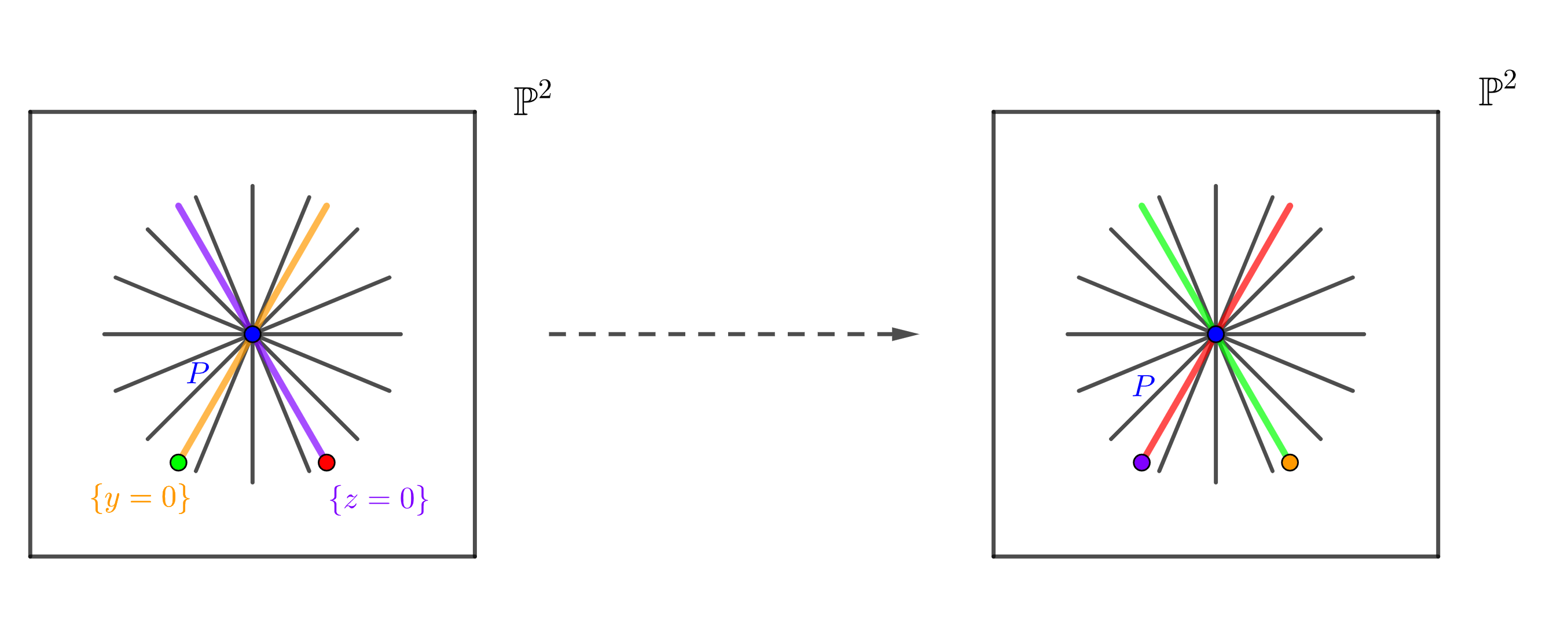
Figure 11: Standard quadratic transformation.

The arguments shown in the proof of [CKS, Theorem 2.30] allow to have the following immediate corollary:

Corollary 3.10.

The centers of de Jonquières transformations obtained from the (volume preserving) Sarkisov Program applied to any element of $\operatorname{Dec}(C)$ belong to the cubic and its strict transform.

We recall that Lemma 3.4 restricts possibilities for the Mori fibered spaces appearing in a volume preserving factorization of $\phi\in\operatorname{Dec}(C)$. This is illustrated by examples in [Alv, Subsection 4.3.1].

The canonical complex of $C\subset\mathbb{P}^{2}$

Let $C\subset\mathbb{P}^{2}$ be an irreducible plane curve (not necessarily nonsingular). We have a complex (not necessarily exact) induced by the natural action $\rho$ of $\operatorname{Dec}(C)$ on $C$

$$1\longrightarrow\operatorname{Ine}(C)\longrightarrow\operatorname{Dec}(C)\overset{\rho}{\longrightarrow}\operatorname{Bir}(C)\longrightarrow 1,$$ (3.1)

where $\operatorname{Ine}(C)$ is identified with $\ker(\rho)$. This complex is called the canonical complex of the pair $(\mathbb{P}^{2},C)$ and the obstruction to its exactness is the surjectivity of $\rho$.

In [BPV1], Blanc, Pan & Vust studied canonical complexes under the usual trichotomy: genera $g\geq 2,g=1$ and $g=0$. See [BPV1] for interesting examples in which the map $\operatorname{Dec}(C)\rightarrow\operatorname{Bir}(C)$ is not surjective. In the case where $C$ is nonsingular, one has $\operatorname{Bir}(C)=\operatorname{Aut}(C)$.

If $g\geq 2$, one can easily check that $C$ has degree $>3$. See [Ful, Proposition 5, Chapter 8]. By the first part in the proof of the Theorem 3.1 or [Pan, Corollaire 3.6], in this case, the group $\operatorname{Dec}(C)$ is trivial in the sense that it is given by the automorphisms of $\mathbb{P}^{2}$ that preserve $C$. That is, if $g\geq 2$, then

$\operatorname{Dec}(C)=\operatorname{Aut}(\mathbb{P}^{2},C)\coloneqq\operatorname{Dec}(C)\cap\operatorname{Aut}(\mathbb{P}^{2})$.

This fact together with the following result due to Matsumura & Monsky [MM] when $n\geq 2$ and Chang [Ch] when $n=1$ implies that the canonical complex of the pair $(\mathbb{P}^{2},C)$ is exact.

Theorem 3.11 (cf. [MM] Theorem 2 and [Ch] Theorem 1).

Let $n$ and $d$ be positive integers and $X$ be a nonsingular hypersurface of degree $d$ in $\mathbb{P}^{n+1}$. If $(n,d)\neq(2,4),(1,3)$, then the natural group homomorphism $\operatorname{Aut}(\mathbb{P}^{n},X)\rightarrow\operatorname{Aut}(X)$ is surjective.

In the case of $d>n$, this result can also be obtained through adjoint systems [Pan, Remarque 3.7]. When $(n,d)=(1,3)$, then $X=C$ is a nonsingular plane cubic. The result by Pan about its decomposition group indicates the existence of nonlinear maps inducing automorphisms of $C$ by restriction. So $\operatorname{Dec}(C)$ is larger than $\operatorname{Aut}(\mathbb{P}^{2},C)$.

In [Bl1], Blanc showed that the inertia group of $C$ is generated by its elements of degree 3, and except for the identity, such elements are the ones with lowest degree. By [Giz, Theorem 6] and [Og, Theorem 2.2] we have that $\operatorname{Aut}(C)$ is no longer derived from $\operatorname{Aut}(\mathbb{P}^{2},C)$, but from $\operatorname{Dec}(C)$. Consequently, this implies the exactness of the canonical complex of $(\mathbb{P}^{2},C)$. From this, we can therefore also describe $\operatorname{Aut}(C)$ as the quotient group $\operatorname{Dec}(C)/\operatorname{Ine}(C)$.

Once we know that a given short complex is exact, we may ask if it splits or not. In [BPV1], Blanc, Pan & Vust posed the problem of splitting or non-splitting of the canonical complex of $(\mathbb{P}^{2},C)$.

Question by Blanc, Pan & Vust.

$C$ is an elliptic curve and therefore also an algebraic group. One has $\operatorname{Aut}(C)=C\rtimes\mathbb{Z}_{d}$, where $C$ is identified with its group of translations and $d\in\{2,4,6\}$, depending on the $j$ invariant of $C$. More precisely, $\mathbb{Z}_{d}\simeq\operatorname{Aut}(C,O)$, the group of automorphisms of $C$ which fix the neutral element $O$ of the group operation of $C$.

Denote by $\oplus$ the group law on $C$ and fix $O\in C$ a neutral element. Given $P\in C\setminus\{O\}$, consider a map $\varphi_{P}\in\operatorname{Dec}(C)$ which by restriction to $C$ induces the translation $T_{P}$ by $P$, that is, $(\varphi_{P})|_{C}(Q)=Q\oplus P$ for all $Q\in C$.

We observe that there are infinitely many maps in $\operatorname{Dec}(C)$ which will induce the same translation $T_{P}$ on $C$. Any composition with an element of $\operatorname{Ine}(C)$ plays the same role. We point out that $\operatorname{Ine}(C)$ as well as $\operatorname{Dec}(C)$ are infinite uncountable groups. This is based on the existence of a free subgroup of the former, their descriptions in terms of presentations and the cardinality of our ground field $\mathbb{C}$. See [Bl1, Theorem 6] and [Pan, Théorèm 1.4].

One can explicitly obtain such a map $\varphi_{P}$, for example, by homogenizing the expressions of the group law on $C$ with affine coordinates in its Weierstrass normal form, and extending them to $\mathbb{P}^{2}$ as a rational map. In what follows we make this explicit.

After a suitable change of coordinates, we can write the equation of $C$ in the Weierstrass normal form as

$y^{2}=x^{3}+px+q,$

where $p,q\in\mathbb{C}$ are not mutually zero, and $(x,y)$ are affine coordinates of $\mathbb{A}^{2}_{(x,y)}=\{z\neq 0\}\subset\mathbb{P}^{2}$. The neutral element $O$ of $\oplus$ is the unique intersection of $C$ with the line at infinity: $O=(0:1:0)$, which is an inflection point.

Let us consider now the translation in $C$ by $(a,b)\in C$. In these coordinates, the group law can be explicitly described as $(x^{\prime},y^{\prime})=(x,y)\oplus(a,b)$ if and only if

$x^{\prime}=\left(\dfrac{y-b}{x-a}\right)^{2}-x-a,~{}y^{\prime}=\dfrac{y-b}{x-a}(x^{\prime}-a)+b$.

Let $\mathbb{P}^{2}$ have homogeneous coordinates $(x:y:z)$. Consider the rational map $\varphi_{P}\colon\mathbb{P}^{2}\dashrightarrow\mathbb{P}^{2}$ defined by the same equations above in the open subset $\{z\neq 0\}$. One can verify birationality and that indeed $\varphi\in\operatorname{Dec}(C)$. In this expression, $\varphi_{P}$ is not defined when $x=a$.

Let us extend $\varphi_{P}$ to the largest possible open subset of $\mathbb{P}^{2}$. Performing some algebraic manipulations and homogenizing, the extension obtained, also denoted by $\varphi_{P}$, becomes

$$\varphi_{P}\colon\mathbb{P}^{2} \dashrightarrow\mathbb{P}^{2}$$

$$(x:y:z) \longmapsto(F_{1}(x,y,z):F_{2}(x,y,z):F_{3}(x,y,z)),$$

with

$$F_{1}(x,y,z) =z(y-bz)^{2}(x-az)-(x^{2}-a^{2}z^{2})(x-az)^{2},$$

$$F_{2}(x,y,z) =z(y-bz)^{3}-(y-bz)(x+2az)(x-az)^{2},$$

$$F_{3}(x,y,z) =z(x-az)^{3}$$

for all $(x:y:z)\in\operatorname{Dom}(\varphi_{P})\coloneqq\mathbb{P}^{2}\setminus\operatorname{Bs}(\varphi_{P})$. One can check that $\operatorname{Bs}(\varphi_{P})=V(F_{1},F_{2},F_{3})=\{P,O\}\subset C$, as predicted by Theorem 3.1.

Let $\Gamma\subset|4H|$ be the linear system associated to $\varphi_{P}$, where $H$ denotes a general line of $\mathbb{P}^{2}$. We have that $\Gamma$ is contained in the linear system of plane quartics passing through $P$ and $O$ with certain multiplicities $m_{P}$ and $m_{O}$, respectively. To compute them, let us make use of the Noether-Fano equations or equations of condition from [Alb, Section 2.5] or [CKS, Theorem 2.9].

These equations imply that we have two possibilities for the multiplicities of a plane birational map of degree $4$ in nonincreasing order, namely, $(3,1,1,1,1,1,1)$ or $(2,2,2,1,1,1)$. Both cases include the multiplicities of the infinitely near base points.

A careful analysis of the general member of $\Gamma$ shows that we are in the first case, with $m_{P}=3$ and $m_{O}=1$. More precisely, $\Gamma$ is contained in the linear system of plane quartics passing through $P$ with multiplicity $3$ and passing through $O$ with multiplicity $1$ and sharing one tangent direction at $O$ and higher order Taylor terms up to order 5. The shared tangent direction is exactly the tangent direction to $C$ at $O$.

Its homaloidal type is $(4;3,1^{6})$, where the coordinate before the semicolon indicates its degree and the further ones in nonincreasing order represent the multiplicities of all base points including the infinitely near ones.

According to [CKS, Definition 2.28(2)], such homaloidal type makes $\varphi_{P}$ a de Jonquières map and the configuration of the seven base points of $\varphi_{P}$ (including the infinitely near ones) is as follows

$P,$

$O\prec P_{1}\prec P_{2}\prec P_{3}\prec P_{4}\prec P_{5},$

where the notation $P_{i}\prec P_{i+1}$ indicates that $P_{i+1}$ is infinitely near to $P_{i}$, that is, each $P_{i}$ belongs to the $i$-th infinitesimal neighborhood of $O$.

By blowing up five times consecutively, we can check that the infinitely near base points $P_{1}\prec P_{2}\prec P_{3}\prec P_{4}\prec P_{5}$ over $O$ are independent of $P$, and the shared tangent directions in the infinitely near points are exactly the tangent directions to the strict transforms of $C$ at them.

We may ask ourselves if $\varphi_{Q\oplus P}=\varphi_{Q}\circ\varphi_{P}$, for all $P,Q\in C\setminus\{O\}$. If this relation is confirmed, it would yield a splitting of the canonical complex of the pair $(\mathbb{P}^{2},C)$ at $C$, coming from a set-theoretical section $\eta\colon C\hookrightarrow\operatorname{Dec}(C)$. In general, the splitting property of a given short exact sequence can be relative to some subgroup and not global. In our context, this subgroup can be continuous or discrete.

Let us investigate the possible set-theoretical section $\eta\colon C\hookrightarrow\operatorname{Dec}(C)$ given by

$\eta(P)=$ $\begin{cases}\varphi_{P},&\text{if $P\neq O$}\\ \operatorname{Id}_{\mathbb{P}^{2}},&\text{otherwise}\end{cases}$.

If $\eta$ is also a group homomorphism, we would have $\varphi_{P}^{-1}=\varphi_{\ominus P}$ for all $P\in C$, where $\ominus P$ denotes the inverse of $P$ under the group law $\oplus$ of $C$.

For all $P,Q\in C\setminus\{O\}$ with $P\neq\ominus Q$, let us compare the degrees of $\varphi_{Q\oplus P}$ and $\varphi_{Q}\circ\varphi_{P}$. We already know that $\deg(\varphi_{Q\oplus P})=4$. The following result will allow us to compute the second degree.

Corollary 3.12 (cf. [Alb] Corollary 4.2.12).

Let $f$ be a plane Cremona map of homaloidal type $(d;m_{1},\ldots,m_{r})$, and let $g$ be a plane Cremona map of homaloidal type $(e;\ell_{1},\ldots,\ell_{s})$ satisfying that the first $k$ base points of $f$ coincide with those of $g$ and no further coincidence. Then the composite map $g\circ f^{-1}$ has degree

$de-\displaystyle\sum_{i=1}^{k}m_{i}\ell_{i}$.

Since $\operatorname{\underline{Bs}}(\varphi_{\ominus P})=\{\ominus P,O\prec P_{1}\prec P_{2}\prec P_{3}\prec P_{4}\prec P_{5}\}$, we have

$\operatorname{\underline{Bs}}(\varphi_{P})\cap\operatorname{\underline{Bs}}(\varphi_{\ominus Q})=\{O\prec P_{1}\prec P_{2}\prec P_{3}\prec P_{4}\prec P_{5}\}$.

Therefore, the previous result tells us that

$\deg(\varphi_{Q}\circ\varphi_{P})=4\cdot 4-6\cdot 1\cdot 1=10\neq 4=\deg(\varphi_{Q\oplus P})$,

which implies that the maps $\varphi_{Q\oplus P}$ and $\varphi_{Q}\circ\varphi_{P}$ are distinct and do not make $\eta$ a group homomorphism.

Thus, our candidate $\eta$ does not yield a splitting of the canonical complex of $(\mathbb{P}^{2},C)$ at $C$. We therefore conclude that we have $\varphi_{Q}\circ\varphi_{P},\varphi_{Q\oplus P}\in\rho^{-1}(T_{Q\oplus P})$ with $\varphi_{Q}\circ\varphi_{P}\neq\varphi_{Q\oplus P}$. This allows us to produce many elements in $\operatorname{Ine}(C)$. For instance, given $P,Q,R\in C$ such that $P\oplus Q\oplus R=O$, then $\varphi_{P\oplus Q}\circ\varphi_{R}$ and $\varphi_{P}\circ\varphi_{Q\oplus R}$ belong to $\operatorname{Ine}(C)$.

In [BF], Blanc & Furter examined topologies and structures of the Cremona groups.

Definition 9 (cf. [BF] Definition 2.1).

Let $A$ and $X$ be irreducible algebraic varieties, and let $f$ be an $A$-birational self-map of the $A$-variety $A\times X$ satisfying the following:

1. $f$ induces an isomorphism $U\overset{\simeq}{\longrightarrow}V$, where $U$ and $V$ are open subsets of $A\times X$, whose projections on $A$ are surjective,

2. $f(a,x)=(a,\operatorname{pr}_{2}(f(a,x)))$, where $\operatorname{pr}_{2}$ denotes the second projection. Hence for each point $a\in A$, the birational map $x\mathrel{\mapstochar\dashrightarrow}\operatorname{pr}_{2}(f(a,x))$ corresponds to an element $f_{a}\in\operatorname{Bir}(X)$.

The map $a\mapsto f_{a}$ represents a map from $A$ to $\operatorname{Bir}(X)$ and it is called a morphism from $A$ to $\operatorname{Bir}(X)$.

These notions yield the following topology on $\operatorname{Bir}(X)$ called the Zariski topology: a subset $F\subset\operatorname{Bir}(X)$ is closed in this topology if for any algebraic variety $A$ and any morphism $A\rightarrow\operatorname{Bir}(X)$, its preimage is closed.

In [BF], Blanc & Furter studied the case where $X=\mathbb{P}^{n}$. Very recently and using more tools, Hassanzadeh & Mostafazadehfard [HM2] investigated similar aspects of $\operatorname{Bir}(X)$ when $X$ is an arbitrary projective variety over an infinite field $k$, of any characteristic and not necessarily algebraically closed.

Observe that a section $\eta\colon C\hookrightarrow\operatorname{Dec}(C)$ induces a $C$-birational self-map $f$ of the $C$-variety $C\times\mathbb{P}^{2}$ in the following way

$$f\colon C\times\mathbb{P}^{2} \dashrightarrow C\times\mathbb{P}^{2}$$

$$(P,x) \longmapsto(P,\eta_{P}(x)),$$

where $\eta_{P}\coloneqq\eta(P)$, for all $P\in C$.

Indeed, for all $P\in C$, the map $\eta_{P}$ is birational. Since $\operatorname{Bs}(\eta_{P})\subset C$ for all $P\in C$ by Theorem 3.1, $f$ determines an isomorphism of $U=V=C\times(\mathbb{P}^{2}\setminus C)$ onto $C\times(\mathbb{P}^{2}\setminus C)$ and therefore satisfies item 1 of Definition 9.

This implies that $\eta$ is a morphism from $C$ to $\operatorname{Bir}(\mathbb{P}^{2})$, whose image is contained in $\operatorname{Dec}(C)$.

More generally, we will show the following which negatively answers the question posed in [BPV1]:

Theorem 3.13.

The canonical complex 3.1 of the pair $(\mathbb{P}^{2},C)$ does not admit any splitting at $C$ when we write $\operatorname{Aut}(C)=C\rtimes\mathbb{Z}_{d}$.

Proof.

For the sake of contradiction, suppose that we have a splitting given by a section $\eta\colon C\hookrightarrow\operatorname{Dec}(C)$. From the above discussion, it follows that $\eta$ is also a morphism from $C$ to $\operatorname{Bir}(\mathbb{P}^{2})$ with respect to the Zariski topology. By [BF, Lemma 2.19], the image $\eta(C)$ of $\eta$ is a closed subgroup of $\operatorname{Bir}(\mathbb{P}^{2})$, which has bounded degree. Thus $C\simeq\eta(C)$ as algebraic varieties, and therefore $\eta(C)$ is a projective algebraic group inside $\operatorname{Bir}(\mathbb{P}^{2})$. However, this violates the fact that any algebraic subgroup of $\operatorname{Bir}(\mathbb{P}^{2})$ is affine [BF, Remark 2.21]. Hence, there does not exist any section $\eta$, which implies the result. ∎

Volume preserving x standard Sarkisov factorization

So far this paper addresses a $2$-dimensional scenario. Within a similar framework in higher dimension, it is natural to ask ourselves about generalizations of Theorem 3.1 and Theorem 3.6, namely,

1. Let $D\subset\mathbb{P}^{n}$ be a hypersurface of degree $n+1$ with canonical singularities and consider $\phi\in\operatorname{Dec}(D)\setminus\operatorname{Aut}(\mathbb{P}^{n},D)$. Does it hold that $\operatorname{Bs}(\phi)\subset D$?

2. In dimension 3 and under the same assumptions, is the Sarkisov algorithm applied to $\phi$ automatically volume preserving?

In dimension $3$, we are dealing with a quartic surface $D\subset\mathbb{P}^{3}$. If $D$ is nonsingular, then it is a K3 surface and $\operatorname{Bir}(D)=\operatorname{Aut}(D)$. In [Og, PQ], there are produced examples of such quartic surfaces for which no nontrivial automorphism is derived from $\operatorname{Bir}(\mathbb{P}^{3})$ by restriction. In these examples, we have $\operatorname{Dec}(D)=\{\operatorname{Id}_{\mathbb{P}^{3}}\}$. Thus, neither of those questions is meaningful in such circumstances. We remark that in this case, $(\mathbb{P}^{3},D)$ is a (t,c) Calabi-Yau pair. The situation changes if we allow strict canonical singularities on $D$. Recall that in this case, by [ACM, Proposition 2.6], we have $\operatorname{Bir}^{\operatorname{vp}}(\mathbb{P}^{3},D)=\operatorname{Dec}(D)$.

Based on the minimal resolution process, the simplest canonical surface singularity is of type $A_{1}$ [KM, Theorem 4.22]. Consider $D\subset\mathbb{P}^{3}$ a general irreducible normal quartic surface having such a type of singularity at $P=(1:0:0:0)$. After suitable coordinate change, one can show that the equation of $D$ is of the form $x_{0}^{2}A+x_{0}B+C$, where $A,B,C\in\mathbb{C}[x_{1},x_{2},x_{3}]$ are general homogeneous polynomials of degrees 2, 3, 4, respectively. Moreover, $A$ is a quadratic form of rank 3.

In the proof of [ACM, Claim 5.8], Araujo, Corti & Massarenti show that the birational involution

$\phi\colon(x_{0}:x_{1}:x_{2}:x_{3})\mapsto(-Ax_{0}-B:Ax_{1}:Ax_{2}:Ax_{3})$

belongs to $\operatorname{Dec}(D)$. One can check that $\operatorname{Bs}(\phi)=V(A,B)$ and it consists of the union of six pairwise distinct lines through $P$ if we take $B$ general enough. This implies that $\operatorname{Bs}(\phi)\not\subset D$ as $D$ does not contain lines. This is in contrast with Theorem 3.1 in dimension 2, which asserts that the base locus is contained in the boundary divisor. This fact will allow us to construct a Sarkisov factorization that is not volume preserving, which shows that a generalization of the Theorem 3.6 does not hold in higher dimensions. Thus, the answer to both initial questions in this section is no.

Let us analyze carefully the map $\phi\in\operatorname{Dec}(D)$. Its associated linear system $\Gamma\subset|\mathcal{O}_{\mathbb{P}^{3}}(3)|$ is in particular contained in the linear system of space cubics passing through the reducible curve $V(A,B)$. Write $V(A,B)=L_{1}\cup\ldots\cup L_{6}$, where each $L_{i}$ stands for a line through $P$.

Consider $\mathcal{H}$ a general member of $\Gamma$. Notice that $P$ is a singularity of $\operatorname{Bs}(\phi)$ as well as of $\mathcal{H}$ and $D$. In particular, we have that $P\in\operatorname{Sing}(\mathcal{H})$ is a canonical singularity of type $A_{1}$ and $m_{P}(\mathcal{H})=2$. This observation will be important later on on many occasions.

Indeed, $\mathcal{H}$ is of the form

$\lambda_{0}(-Ax_{0}-B)+\lambda_{1}Ax_{1}+\lambda_{2}Ax_{2}+\lambda_{3}Ax_{3}$,

for some $(\lambda_{0}:\lambda_{1}:\lambda_{2}:\lambda_{3})\in\mathbb{P}^{3}$ identified with $\Gamma$.

Dehomogenizing $\mathcal{H}$ with respect to $x_{0}$, we get the equation of $\mathcal{H}$ in $\{x_{0}\neq 0\}$ becomes

$\lambda_{0}(-A-B)+\lambda_{1}Ax_{1}+\lambda_{2}Ax_{2}+\lambda_{3}Ax_{3}$.

Thus, $TC_{P}\mathcal{H}=\{-\lambda_{0}A=0\}$ whose projectivization is an irreducible conic, since $\operatorname{rank}(A)=3$. We can assure that $P\in\operatorname{Sing}(\mathcal{H})$ is of type $A_{1}$ because a single blowup of the ambient space will be enough to resolve the singularity. One can check that the corresponding exceptional divisor intersected with the strict transform of $\mathcal{H}$ is an irreducible conic.

Another way to argue why $P\in\operatorname{Sing}(\mathcal{H})$ is of type $A_{1}$ is by looking at $TC_{P}\mathcal{H}$ and comparing it with the tangent cones of normal forms of surface canonical singularities. We would be using the fact that canonical singularities are equivalent to rational double points in dimension 2.

Let us run the Sarkisov Program for $\phi$. From now on we will follow the notation and algorithm described in [Cor1]. Although it has a slightly different notation, we refer the reader to [Mat, Flowchart 13-1-9] for an explicit flowchart.

Notation.

Henceforth, abusing notation, sometimes we will denote divisors on varieties and their strict transforms or pushforwards in others with the same symbol. Moreover, to avoid confusion in some instances, we will denote certain strict transforms or pushforwards with a right lower index indicating the ambient variety. We will do the same for general members of linear systems.

We will exhibit in detail a possible Sarkisov factorization for $\phi$ proceeding in steps. Similarly to the surface case, there also exists a notion of Sarkisov degree to detect the complexity of a birational map between threefolds with the structure of Mori fibered space. The point here is that it consists now of a triple of values and not a single one as in Definition 5. We will briefly expose this notion, referring the reader to [Cor1, Mat] for more explicit and precise definitions.

Definition 10 (cf. [Cor1] Definition 5.1).

Let

be a birational map between threefold Mori fibered spaces. Consider the choice of $\mathcal{H}$ and $\mathcal{H^{\prime}}$ made in [Cor1, Section 4]. The Sarkisov degree of $(\mathcal{H},~{}f\colon X\rightarrow S)$ is the triple $(\mu,c,e)$ where

1. $\mu$ is the quasi-effective threshold defined by $\mathcal{H}\equiv-\mu K_{X}$ over $S$ as in [Cor1, Section 4];

2. $c$ is the canonical threshold of the pair $(X,\mathcal{H})$;

3. $e$ is the number of crepant exceptional divisors with respect to the pair $(X,c\mathcal{H})$.

If $X^{\prime}\overset{f^{\prime}}{\longrightarrow}S^{\prime}$ is $\mathbb{P}^{3}\rightarrow\operatorname{Spec}(\mathbb{C})$, then $\mathcal{H}$ can be seen as a general member of the linear system associated to $\phi\colon X\dashrightarrow\mathbb{P}^{3}$.

On the set of triples $(\mu,c,e)$ we introduce a partial ordering as follows:

$(\mu,c,e)>(\mu_{1},c_{1},e_{1})$ if either

1. $\mu>\mu_{1}$, or

2. $\mu=\mu_{1}$ and $c<c_{1}$ (no mistype here), or

3. $\mu=\mu_{1},c=c_{1}$ and $e>e_{1}$.

The starting point or Step 0 in the Sarkisov Program is to compute the Sarkisov degree $(\mu,c,e)$ of the corresponding birational map $\phi$. It will guide us along the factorization process. Performing a lot of computations, one can find that the Sarkisov degree of $\phi$ is $\left(\dfrac{3}{4},1,9\right)$.

Extend the notion of infinitesimal neighborhood, as defined in [CKS, Section 2.2], analogously in higher dimension and for subvarieties other than closed points. The 9 crepant exceptional divisors with respect to the pair $(\mathbb{P}^{3},c\mathcal{H})=(\mathbb{P}^{3},\mathcal{H})$ are the exceptional divisors corresponding to the blowups of

• $P$,

• a curve $e$ in the first infinitesimal neighborhood of $P$,

• a curve $e^{\prime}$ in the first infinitesimal neighborhood of $e$ and

• of the six lines $L_{1},\ldots,L_{6}$.

Step 1:

Following the Sarkisov algorithm in [Cor1], since $c=1<\dfrac{4}{3}=\dfrac{1}{\mu}$, the first link in the Sarkisov factorization is of type I or II. This link is initiated by an extremal blowup [Cor1, Proposition-Definition 2.10], which always exists in this situation.

This choice of the extremal blowup is not determined by the algorithm. We are free to choose it. In our case, we have seven possibilities for such maps which are the blowup of $\mathbb{P}^{3}$ at $P$ or the blowup of $\mathbb{P}^{3}$ along one of the lines $L_{i}$ through $P$.

Only the first option gives us a volume preserving map, whereas the remaining ones do not. Indeed, let $\sigma_{P}\colon Z_{1}\rightarrow\mathbb{P}^{3}$ be the blowup of $P$ and set $E_{P}\coloneqq\operatorname{Exc}(\sigma_{P})$. By the Adjunction Formula, we have $K_{Z_{1}}=\sigma_{P}^{*}K_{\mathbb{P}^{3}}+2E_{P}$ and because $m_{P}(D)=2$, we have $D_{Z_{1}}\sim\sigma_{P}^{*}D-2E_{P}$. Hence,

$K_{Z_{1}}+D_{Z_{1}}=\sigma_{P}^{*}(K_{\mathbb{P}^{3}}+D)$,

and since $(\sigma_{P})_{*}D_{Z_{1}}=D$, Proposition 2.1 implies that $\sigma_{P}$ is volume preserving.

Without less of generality, let $\sigma_{1}\colon Z_{1}^{\prime}\rightarrow\mathbb{P}^{3}$ be the blowup of $L_{1}$ and set $E_{1}\coloneqq\operatorname{Exc}(\sigma_{1})$. By the Adjunction Formula, we have $K_{Z_{1}^{\prime}}=\sigma_{1}^{*}K_{\mathbb{P}^{3}}+E_{1}$ and because $L_{1}\not\subset D$, we have $D_{Z_{1}^{\prime}}\sim\sigma_{1}^{*}D$. Hence,

$K_{Z_{1}^{\prime}}+D_{Z_{1}^{\prime}}=\sigma_{1}^{*}(K_{\mathbb{P}^{3}}+D)+E_{1}$.

Notice that $(K_{Z_{1}^{\prime}},D_{Z_{1}^{\prime}})$ is no longer a Calabi-Yau pair. For the sake of contradiction, suppose that $\sigma_{1}$ is volume preserving for some reduced Weil divisor $D_{1}$ on $Z_{1}^{\prime}$ making $(K_{Z_{1}^{\prime}},D_{1})$ a Calabi-Yau pair. One has $a(E_{1},\mathbb{P}^{3},D)=1$ by the previous formula, and hence we must have $a(E_{1},Z_{1}^{\prime},D_{1})=1$. Since $E_{1}\subset Z_{1}^{\prime}$, by definition of discrepancy this implies the $E_{1}\subset\operatorname{Supp}(D_{1})$ and it has coefficient $-1$. But this is absurd because we are assuming $D_{1}$ reduced. Therefore, $\sigma_{1}$ is not volume preserving.

Let us proceed with $\sigma_{P}$. Consider $\mathcal{H}$ a general member of the linear system associated to $\phi$. Since $c=1$, the next thing to do is to run the $(K_{Z_{1}}+\mathcal{H}_{Z_{1}})$-MMP over $\operatorname{Spec}(\mathbb{C})$. One can verify it results in the Mori fibered space structure $\pi_{1}\colon Z_{1}\rightarrow\mathbb{P}^{2}$.

Thus, the first (volume preserving) Sarkisov link in a factorization of $\phi$ is of type I, and it is given by the blowup of $\mathbb{P}^{3}$ at $P$. We have that $E_{P}\simeq\mathbb{P}^{2}$, $\tilde{A}\simeq\mathbb{F}_{2}$ and (by abuse of notation) $e=E_{P}\cap D_{Z_{1}}\simeq\mathbb{P}^{1}$. Moreover, the curve $e$ is contained in $\operatorname{Bs}(\phi\circ\sigma_{P})$. All the lines $L_{i}$ are separated in $Z_{1}$ and are, in particular, rulings of $\mathbb{F}_{2}$. Observe that $\pi_{1}$ maps $e$ isomorphically onto the conic $\{A=0\}\subset\mathbb{P}^{2}$. We have the following picture:

Figure 12: First link in a Sarkisov factorization of $\phi$.

Step 2:

We must compute the Sarkisov degree $(\mu_{1},c_{1},e_{1})$ of the induced birational map $\phi\circ\sigma_{P}$. One can check that it equals $\left(\dfrac{1}{2},1,8\right)$ and it is smaller than $(\mu,c,e)$ according to the partial ordering explained after the Definition 10. So the birational map $\phi\circ\sigma_{P}$ is “simpler” than $\phi$.

Since $c_{1}=1<2=\dfrac{1}{\mu_{1}}$, the second link in the Sarkisov factorization is of type I or II. At this point, we also have seven extremal blowups to choose from. They are the blowup of $Z_{1}$ along $e$ or the blowup of $Z_{1}$ along one of the lines $L_{i}$. Repeating exactly the same arguments as in Step 1, we can check that the first one yields a volume preserving map whereas the remaining ones do not. The reason behind this is that $e\subset D_{Z_{1}}$ and $L_{i}\not\subset D_{Z_{1}}$ for all $i\in\{1,\ldots,6\}$.

Let us continue with $\sigma_{e}\colon Y_{1}\rightarrow Z_{1}$ the blowup of $Z_{1}$ along $e$ and set $E_{e}\coloneqq\operatorname{Exc}(\sigma_{e})$.

By [Har, Theorem 8.24, (b)], we have that $E_{e}\simeq\mathbb{P}(\mathcal{N}_{e/Z_{1}}^{\vee})$. One can compute $\mathcal{N}_{e/Z_{1}}^{\vee}\simeq\mathcal{O}_{\mathbb{P}^{1}}(2)\oplus\mathcal{O}_{\mathbb{P}^{1}}(-4)$ and therefore $E_{e}\simeq\mathbb{F}_{6}$.

The curve $e^{\prime}=E_{e}\cap D_{Y_{1}}\simeq\mathbb{P}^{1}$ is contained in $\operatorname{Bs}(\phi\circ\sigma_{P}\circ\sigma_{e})$. Roughly speaking, we can say that $e^{\prime}$ is an infinitely near curve to $e$ in analogy with the notion of infinitely near points in dimension 2. See [CKS, Section 2.2].

Since $c_{1}=1$, we need to run the $(K_{Y_{1}}+\mathcal{H}_{Y_{1}})$-MMP over $\mathbb{P}^{2}$.

One can verify that this log MMP results in the divisorial contraction

$\alpha\colon Y_{1}\rightarrow Z_{2}\simeq\mathbb{P}(\mathcal{O}_{\mathbb{P}^{2}}\oplus\mathcal{O}_{\mathbb{P}^{2}}(3))$,

where $\pi_{2}\colon Z_{2}\rightarrow\mathbb{P}^{2}$ is the corresponding structure morphism making $Z_{2}$ a Mori fibered space. This birational morphism contracts exactly the rulings of $\tilde{A}\simeq\mathbb{F}_{2}$, that is, $\tilde{A}=\operatorname{Exc}(\alpha)$. The isomorphism $Z_{2}\simeq\mathbb{P}(\mathcal{O}_{\mathbb{P}^{2}}\oplus\mathcal{O}_{\mathbb{P}^{2}}(3))$ may be justified by analyzing the section of $\pi_{2}$ given by $\mathbb{P}^{2}\rightarrow E_{P}\simeq\mathbb{P}^{2}$; and by $K_{Z_{2}}=\alpha_{*}K_{Y_{1}}$ written in terms of a basis for $\operatorname{Pic}(Z_{2})$ and comparing it with the formula for the canonical class of a projective bundle.

Thus, the second (volume preserving) Sarkisov link in a factorization of $\phi$ is of type II, and it is given by the composition $\alpha\circ\sigma_{e}^{-1}$. Observe that $\alpha$ maps $E_{e}$ isomorphically, via pushforward, onto the cylinder $E_{e}=\{A=0\}\subset Z_{2}$. In particular, all the lines $L_{i}$ are contracted by $\alpha$. Moreover, we have that $\operatorname{Bs}(\phi\circ\sigma_{P}\circ\sigma_{e}\circ\alpha^{-1})$ consists of the curve $f=\alpha(e^{\prime})$ which is mapped by $\pi_{2}$ isomorphically onto the conic $\{A=0\}\subset\mathbb{P}^{2}$. We have the following picture in which we did not put the strict transforms of $D$ to not pollute it:

Figure 13: Second link in a Sarkisov factorization of $\phi$.

Notice that we have similar behavior to the elementary transformations between the Hirzebruch surfaces $\mathbb{F}_{n}\simeq\mathbb{P}(\mathcal{O}_{\mathbb{P}^{1}}\oplus\mathcal{O}_{\mathbb{P}^{1}}(n))$. Indeed, by [Har, Example 2.11.4] one has $Z_{1}\simeq\mathbb{P}(\mathcal{O}_{\mathbb{P}^{2}}\oplus\mathcal{O}_{\mathbb{P}^{2}}(1))$. The composition $\alpha\circ\sigma_{e}^{-1}$ is the blowup along $e$ followed by the contraction of the birational transforms of all fibers of $\pi_{1}$ through $e$, which correspond to the rulings of $\tilde{A}\simeq\mathbb{F}_{2}$. Geometrically, we have only interchanged a family of fibers of $\pi_{2}$ parameterized by $e\simeq\mathbb{P}^{1}$.

Step 3:

Once again, we need to compute the Sarkisov degree $(\mu_{2},c_{2},e_{2})$ of the induced birational map $\phi\circ\sigma_{P}\circ\sigma_{e}\circ\alpha^{-1}$. One can check that equals $\left(\dfrac{1}{2},1,1\right)$ and it is smaller than $(\mu_{1},c_{1},e_{1})$. Thus we have simplified the birational map $\phi\circ\sigma_{P}$.

Since $c_{2}=1<2=\dfrac{1}{\mu_{2}}$, the third link in the Sarkisov factorization is of type I or II. The difference in this step is that we have only one possible extremal blowup given by the blowup of $Z_{2}$ along $f$. Consider $\sigma_{f}\colon Y_{2}\rightarrow Z_{2}$ such map and denote $E_{f}\coloneqq\operatorname{Exc}(\sigma_{f})$.

As in the previous steps, the map $\sigma_{f}$ is volume preserving because $f\subset D_{Z_{2}}$. One can check that the map $\phi\circ\sigma_{P}\circ\sigma_{e}\circ\alpha^{-1}\circ\sigma_{f}$ is everywhere defined.

Since $c_{1}=1$, we need to run the $(K_{Y_{2}}+\mathcal{H}_{Y_{2}})$-MMP over $\mathbb{P}^{2}$. By [Har, Theorem 8.24, (b)], we have that $E_{f}\simeq\mathbb{P}(\mathcal{N}_{f/Z_{2}}^{\vee})$. One can compute $\mathcal{N}_{f/Z_{2}}^{\vee}\simeq\mathcal{O}_{\mathbb{P}^{1}}(6)\oplus\mathcal{O}_{\mathbb{P}^{1}}(4)$ and therefore $E_{f}\simeq\mathbb{F}_{2}$.

Repeating the same arguments as in Step 2, we obtain a divisorial contraction $\beta\colon Y_{2}\rightarrow Z_{3}\simeq\mathbb{P}(\mathcal{O}_{\mathbb{P}^{2}}\oplus\mathcal{O}_{\mathbb{P}^{2}}(1))$. The third (volume preserving) Sarkisov link in a factorization of $\phi$ is of type II, and it is given by the composition $\beta\circ\sigma_{f}^{-1}$ with analogous geometric properties to the previous one. We have the following picture:

Figure 14: Third link in a Sarkisov factorization of $\phi$.

Step 4:

The computation of the Sarkisov degree of the induced birational map $\phi\circ\sigma_{P}\circ\sigma_{e}\circ\alpha^{-1}\circ\sigma_{f}\circ\beta^{-1}$ will be a little different. The issue here is that the pair $(Z_{3},c\mathcal{H}_{Z_{3}})$ is canonical for any positive rational number $c$, since $\mathcal{H}_{Z_{3}}$ is base point free. So the notion of canonical threshold would lead us to $c_{3}~{}\text{``$=$''}~{}\infty$. This is in accordance with Definition 10.

In this case, the Sarkisov degree $(\mu_{3},c_{3},e_{3})$ becomes $\left(\dfrac{1}{2},\infty,*\right)$ and it is smaller than $(\mu_{2},c_{2},e_{2})$.

Since $c_{3}=\infty\ \text{``$\geq$''}\ 2=\dfrac{1}{\mu_{3}}$, the fourth link in the Sarkisov factorization is of type III or IV. We need to run the $(K_{Z_{3}}+2\mathcal{H}_{Z_{3}})$-MMP over $\operatorname{Spec}(\mathbb{C})$. This log MMP results exactly in the divisorial contraction given by the blowup of $\mathbb{P}^{3}$ at $P$, that is, the map $\sigma_{P}$. We observe that $E_{f}$ is precisely $\operatorname{Exc}(\sigma_{P})$.

One can compute that the Sarkisov degree $(\mu_{4},c_{4},e_{4})$ of the induced birational map $\phi\circ\sigma_{P}\circ\sigma_{e}\circ\alpha^{-1}\circ\sigma_{f}\circ\beta^{-1}\circ\sigma_{P}^{-1}$ is $\left(\dfrac{1}{4},\infty,*\right)$, which is smaller than the previous one. Such Sarkisov degree implies that this map is an automorphism of $\mathbb{P}^{3}$.

The (volume preserving) factorization of $\phi$ is ended up by the Sarkisov link of type III given by $\sigma_{P}$. We have the following picture:

Figure 15: Fourth link in a Sarkisov factorization of $\phi$.

We observe that the strict transforms of $D$ remained nonsingular and isomorphic to $D$ along the intermediate steps. In terms of a commutative diagram, this volume preserving factorization of $\phi$ is expressed in the following way:

We have the following sequence of Sarkisov degrees of the induced birational maps:

$\left(\dfrac{3}{4},1,9\right)>\left(\dfrac{1}{2},1,8\right)>\left(\dfrac{1}{2},1,1\right)>\left(\dfrac{1}{2},\infty,*\right)>\left(\dfrac{1}{4},\infty,*\right)$.

Non-volume preserving factorization of $\phi$:

Let us make some comments if instead of proceeding with $\sigma_{e}$ in Step 2, we had chosen $\sigma_{1}$. We invite the reader to fill out the details and make drawings in order to see what is happening geometrically.

For $i\in\{1,\ldots,6\}$, denote $P_{i}\coloneqq L_{i}\cap E_{P}$. In this other Sarkisov factorization the $(i+1)$-th Sarkisov link is of type I, and it is given by $\sigma_{i}\colon\operatorname{Bl}_{L_{1},\ldots,L_{i}}(Z_{1})\rightarrow\operatorname{Bl}_{L_{1},\ldots,L_{i-1}}(Z_{1})$, where $\operatorname{Bl}_{L_{1},\ldots,L_{i}}(Z_{1})\rightarrow\operatorname{Bl}_{P_{1},\ldots,P_{i}}(\mathbb{P}^{2})$ is the corresponding structure of Mori fibered space. One can show that $E_{i}\coloneqq\operatorname{Exc}(\sigma_{i})$ is isomorphic to $\mathbb{F}_{0}\simeq\mathbb{P}^{1}\times\mathbb{P}^{1}$ for all $i\in\{1,\ldots,6\}$.

We have the following picture for $\sigma_{1}$, where $g=\tilde{E_{P}}\cap E_{1}\simeq\mathbb{P}^{1}$. Geometrically, $g$ represents all the normal directions to $L_{1}$ at $P_{1}$.

Figure 16: Sarkisov link $\sigma_{1}$.

After $\sigma_{6}$, the next two Sarkisov links are analogous to the intermediate ones in the volume preserving factorization described previously. In particular, they are volume preserving Sarkisov links of type II.

Finally, the remaining ones are given by the consecutive blowdowns of the corresponding strict transforms of $E_{1},\ldots,E_{6}$ and $E_{P}$, respectively. All of them are Sarkisov links of type III and the last one is volume preserving. The setting is depicted in Figure 17.

Figure 17: Blowdowns of the $E_{i}$’s.

We have the following sequence of Sarkisov degrees of the induced birational maps:

$\left(\dfrac{3}{4},1,9\right)>\underbrace{\left(\dfrac{1}{2},1,8\right)>\ldots>\left(\dfrac{1}{2},1,2\right)}_{\text{relative to the $\sigma_{i}$'s}}>\left(\dfrac{1}{2},1,1\right)>\underbrace{\left(\dfrac{1}{2},2,6\right)>\ldots>\left(\dfrac{1}{2},2,1\right)}_{\text{relative to the blowdowns of the $E_{i}$'s}}$

$>\left(\dfrac{1}{2},\infty,*\right)>\left(\dfrac{1}{4},\infty,*\right)$.

We remark that it is relevant that $P\in\operatorname{Sing}(\mathcal{H})$ is a singularity of type $A_{1}$ for the increasing of the canonical threshold in Step 8. The induced birational map before the Sarkisov links of type III has a base locus given by $\{P_{1},\ldots,P_{6}\}$.

Conclusion

By the previous detailed example, we can see the existence of a Sarkisov factorization for a volume preserving map that is not automatically volume preserving. This means that Theorem 3.6 is very particular for dimension 2.

The point is that the volume preserving factorization assured by [CK, Theorem 1.1] is induced by a standard Sarkisov factorization constructed in a special way [CK, Theorem 3.3]. But this special factorization may not be obtained by following algorithmically the Sarkisov Program, at least in dimension 3, if we make certain choices along the process.

In a careful analysis of the volume preserving decomposition of $\phi$ exhibited in [ACM], we show that it can be obtained by choosing conveniently the centers of the extremal blowups initiating Sarkisov links of type I and II. Furthermore, this factorization has the effect of resolving the map $\phi$ along the process as a consequence of the untwisting of the Sarkisov degree of the induced birational maps.

References

• [ACM] C. Araujo, A. Corti, A. Massarenti, Birational geometry of Calabi–Yau pairs and $3$-dimensional Cremona transformations, 2023. arXiv preprint: 2306.00207v2.
• [Alb] M. Alberich-Carramiñana, Geometry of the plane Cremona maps, Lecture Notes in Mathematics 1769, Springer-Verlag, 2002, Berlin.
• [Alv] E. Alves, Log Calabi-Yau geometry and Cremona maps, PhD thesis, IMPA, 2023.
• [Ar] C. Araujo, Introduction to the Minimal Model Program in Algebraic Geometry, IV Congreso Latinoamericano de Matemáticos, 2012. Córdoba, Argentina.
• [BB] L. Bayle, A. Beauville, Birational involutions of $\mathbb{P}^{2}$, Asian J. Math. 4 , no. 1, 2000, 11-18.
• [Bea] A. Beauville, Complex Algebraic Surfaces, London Mathematical Society Student Texts, 34 2nd ed., 1996. Cambridge: Cambridge University Press.
• [BF] J. Blanc, J. Furter, Topologies and structures of the Cremona groups, Ann. of Math., 178(2), 2013, no. 3, 1173–1198.
• [Bl1] J. Blanc, On the inertia group of elliptic curves in the Cremona group of the plane, Michigan Math. J. 56(2), 2008, 315–330.
• [Bl2] J. Blanc, Symplectic birational transformations of the plane, Osaka J. Math., 50(2), 2013, 573-590.
• [BPV1] J. Blanc, I. Pan, T. Vust, On birational transformations of pairs in the complex plane, Geom. Dedicata 139, 2009, 57–73.
• [BPV2] J. Blanc, I. Pan, T. Vust, Sur un Théorème de Castelnuovo, Bull. Braz. Math. Soc., New Series 39, 2008, 61–80.
• [Cas] G. Castelnuovo, Sulle transformazioni cremoniane del piano, che ammettono una curva fissa, Rend. Accad. Lincei (1892) ; Memorie scelte, Zanichelli, 1937, Bologna.
• [Ch] H. C. Chang, On Plane Algebraic Curves, Chinese Journal of Mathematics, 6(2), 1978, 185-189.
• [CK] A. Corti, A.-S. Kaloghiros, The Sarkisov program for Mori fibred Calabi–Yau pairs, Alg. Geom., 3(3), 2016, 370-384.
• [CKS] A. Corti, J. Kollár, K. E. Smith, Rational and nearly rational varieties, Cambridge studies in advanced Mathematics, 92, 2004. With the collaboration of C. H. Clemens and A. Corti.
• [Cor1] A. Corti, Factoring birational maps of threefolds after Sarkisov, J. Algebraic Geom. 4(2), 1995, 223–254.
• [Cor2] A. Corti, Singularities of linear systems and 3-fold birational geometry, in Explicit birational geometry of 3-folds, 281 of London Math. Soc. Lecture Note Ser., 2000, 259–312. Cambridge Univ. Press, Cambridge.
• [Des1] J. Deserti, Some properties of the Cremona group, Ensaios Matemáticos, 21, Sociedade Brasileira de Matemática, 2012. Rio de Janeiro.
• [Des2] J. Deserti, The Cremona group and its subgroups, Mathematical Surveys and Monographs, 252. American Mathematical Society, 2021. Providence, RI.
• [DHZ] T. Ducat, I. Heden, S. Zimmermann, The decomposition groups of plane conics and plane rational cubics, Math. Res. Lett., 26(1), 2019, 35-52.
• [Ful] W. Fulton, Algebraic Curves, An Introduction to Algebraic Geometry, 3rd ed., 2008. Available online.
• [Giz] M. H. Gizatullin, The decomposition, inertia and ramification groups in birational geometry, Algebraic Geometry and Its Applications, Aspects of Mathematics 25, 1994, 39–45.
• [Har] R. Hartshorne, Algebraic Geometry, Graduate Texts in Mathematics, 52, 2013, New York: Springer Science and Business Media.
• [HM1] C. D. Hacon and J. McKernan, The Sarkisov program, J. Algebraic Geom. 22(2), 2013. 389–405.
• [HM2] S. H. Hassanzadeh, M. Mostafazadehfard, $\operatorname{Bir}(X)_{d}$ is constructible, 2022. arXiv preprint: 2208.12333.
• [HZ] I. Heden, S. Zimmermann, The decomposition group of a line, Proc. Amer. Math. Soc. 145, 2017, no. 9, 3665-3680.
• [Lam] S. Lamy, The Cremona Group, book in preparation.
• [KM] J. Kollár, S. Mori, Birational geometry of algebraic varieties, Cambridge Tracts in Mathematics, 134, 1998. With the collaboration of C. H. Clemens and A. Corti.
• [Kol] J. Kollár, Singularities of the Minimal Model Program, Cambridge Tracts in Mathematics, CUP, 200, 2013. With the collaboration of S. Kovács.
• [Mat] K. Matsuki, Introduction to the minimal model program, Universitext, 2002. New York.
• [MM] H. Matsumura, P. Monsky, On the automorphisms of hypersurfaces J. Math. Kyoto Univ., 3, 1963/1964, 347-361.
• [Og] K. Oguiso, Smooth quartic K3 surfaces and cremona transformations, II, 2011. arXiv preprint: 2202.04244.
• [Pan] I. Pan, Sur le sous-groupe de décomposition d’une courbe irrationnelle dans le groupe de Cremona du plan, Michigan Math. J., 55, 2007, 285-298.
• [Piñ] S. Piñeros, The Decomposition Group of Plane Curves, Master dissertation, IMPA, 2019.
• [PQ] D. Paiva, A. Quedo, Automorphisms of quartic surfaces and Cremona transformations, 2023. arXiv preprint: 2302.09014.
• [Rei] M. Reid, Chapter on algebraic surfaces. IAS/Park City Mathematical Series 3, 1997. In Complex Algebraic Geometry, Amer. Math. Soc.