Scene Prior Filtering for Depth Map Super-Resolution

Abstract

Multi-modal fusion is vital to the success of super-resolution of depth maps. However, commonly used fusion strategies, such as addition and concatenation, fall short of effectively bridging the modal gap. As a result, guided image filtering methods have been introduced to mitigate this issue. Nevertheless, it is observed that their filter kernels usually encounter significant texture interference and edge inaccuracy. To tackle these two challenges, we introduce a Scene Prior Filtering network, SPFNet, which utilizes the priors surface normal and semantic map from large-scale models. Specifically, we design an All-in-one Prior Propagation that computes the similarity between multi-modal scene priors, i.e., RGB, normal, semantic, and depth, to reduce the texture interference. In addition, we present a One-to-one Prior Embedding that continuously embeds each single-modal prior into depth using Mutual Guided Filtering, further alleviating the texture interference while enhancing edges. Our SPFNet has been extensively evaluated on both real and synthetic datasets, achieving state-of-the-art performance. Project page: https://yanzq95.github.io/projectpage/SPFNet/index.html.

1 Introduction

Advances in sensor technology have led to the extensive application of depth cues in various fields, such as autonomous driving [47, 1, 38, 36, 44], 3D reconstruction [13, 28, 41, 43, 39], and virtual reality [17, 42, 30, 54, 33]. However, depth measurements are typically low resolution (LR) due to sensor limitations and the complexity of imaging environments. Recently, a number of guided image filtering approaches [20, 14, 51, 5, 32] are proposed to facilitate depth map super-resolution (DSR). Nevertheless, the filter kernels, which are constructed directly from RGB images, often suffer from significant texture interference, and the clarity near edges is typically compromised. For instance, as shown in Fig. 1(e) and (f) (yellow boxes), the filter kernels of DKN [14] and DAGF [51] contain a substantial amount of textures. Fig. 1(i) shows that these two kernels display too many abrupt changes, while the ground truth depth is considerably smoother. These observations show that the texture interference is not conducive to depth recovery. Moreover, within the white boxes, the edges and their neighboring pixels show a high degree of similarity, leading to an insufficient contrast.

Compared to the RGB input, Fig. 1(b) indicates that the surface normal is largely devoid of texture interference. On the other hand, Fig. 1(c) shows that the semantic map displays clear edges between different categories. These inherent characteristics are highly advantageous for constructing filter kernels with less texture interference and more distinct edges.

Figure 1: Visual results of scene priors and filter kernels. The normal (Nor.) (b) and semantic (Sem.) (c) are produced from (a) using Omnidata [6] and SAM [16], respectively. (e) and (f) are the filter kernels derived from DKN [14] and DAGF [51], while (g) and (h) are from our SPFNet. (i) is the normalized kernel distribution.

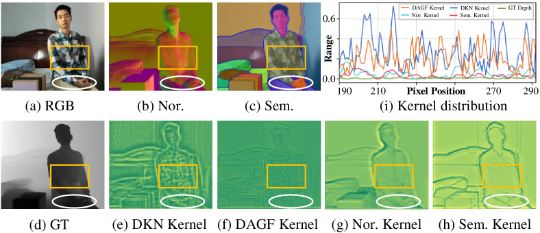
Drawing from the observations above, we design a Scene Prior Filtering Network (SPFNet) to reduce texture interference and enhance edge accuracy. Specifically, we first employ large-scale models, i.e., Omnidata [6] and SAM [16], to generate normal and semantic priors from RGB input. An all-in-one prior propagation (APP) is introduced, which computes the similarity between multi-modal scene priors, i.e., RGB, normal, semantic, and depth, to weaken the texture interference. In addition, we present a one-to-one prior embedding (OPE) that sequentially incorporates each single-modal prior into depth using Mutual Guided Filtering (MGF), further diminishing the interference and enhancing edges via normal and semantic. The MGF comprises a bidirectional path, that is, prior-to-depth filtering and depth-to-prior filtering. The prior-to-depth filtering is to transfer the accurate structural components from scene priors to depth. Conversely, the depth-to-prior filtering leverages depth knowledge to accentuate the edges of these scene priors, while downplaying the undesired textures.

As a result, Fig. 1(g) and (h) show that, the kernels produced by our SPFNet are largely resistant to interference and exhibit precise edges. Furthermore, Fig. 1(i) shows that the distribution of our normal and semantic filter kernels aligns more closely with the ground truth, as compared to DKN and DAGF. The main contributions of this work are:

• To address the issues of texture interference and edge inaccuracy in DSR, we are pioneering the incorporation of scene priors from large-scale models.

• We propose SPFNet, which recursively implements the novel APP, OPE, and MGF to further diminish the texture interference and enhance edges.

• Extensive experimental results demonstrate that our SPFNet achieves superior performance, reaching the state of the art.

2 Related Work

Multi-modal fusion based DSR. Much progress in guided DSR [12, 31, 8, 50, 43, 37] based on deep learning has been made in recent years. Deng et al. [4] utilize multi-modal convolutional sparse coding to extract the common feature between RGB and depth. Zhao et al. [48] develop spherical space feature decomposition to separate domain-shared and domain-private features. In [10], He et al.exploit octave convolution [2] to adaptively decompose the RGB feature into high-frequency and low-frequency components. Similarly, Yuan et al. [42] introduce a deep contrast network to split the depth into high-frequency and low-frequency maps. Most recently, a few methods [49, 23, 33, 26, 3] exploit depth structure scene recovery. For instance, Metzger et al. [23] combine anisotropic diffusion and deep convolutional network to improve the edge transferring property of diffusion. Wang et al. [33] design a structure-guided network that employs the gradient and frequency domains for structure enhancement. Different from previous methods that directly transform RGB to depth, we focus on leveraging surface normal and semantic priors to attenuate texture interference and improve the accuracy near edges.

Guided image filtering based DSR. To transfer the structure information from guidance to target, numerous guided image filtering methods  [19, 9, 20, 29, 52, 14, 51] have been proposed in recent years. Li et al. [20] develop joint image filtering based on deep convolutional networks to selectively transfer the structure from RGB to depth, and Kim et al. [14] present a deformable kernel network that explicitly generates a spatially-variant filter kernel and outputs sets of the neighborhoods for each pixel. In [32], Wang et al. utilize the hybrid side window filtering to propagate multi-scale structure knowledge from RGB to depth. In addition, several methods [5, 51, 45] explore the mutual dependencies between the guidance and target. For example, Dong et al. [5] design a cross-domain adaptive filter to achieve mutual modulation of multi-modal inputs, and Zhong et al. [51] combine filter kernels from the guidance and target to model pixel-wise dependency between the two images. In contrast, we focus on minimizing texture interference within the filter kernel and improving the accuracy of the edges, achieved by exploiting scene priors and similarity maps.

Normal and semantic awareness. Surface normal and semantic priors contain rich geometry and boundary information. Thus, a number of methods [6, 35, 24, 16, 34, 18] leverage these priors for depth recovery. Xu et al. [35] learn the geometric constraints between depth and surface normal in a diffusion module to improve the performance of depth completion. On the other hand, Qiu et al. [24] integrate guided image and surface normal to enhance the depth accuracy, and Fan et al. [7] present a data-fusion CNN method that fuses inferred surface normal and image for accurate free space detection. In addition, Wu et al. [34] develop a semantic-aware knowledge-guided model to embed semantic prior in feature representation space for low-light image enhancement. In this work, we leverage large-scale models to generate accurate surface normal and semantic priors from HR RGB, both of which are utilized to alleviate texture interference and promote the quality of depth restoration.

Figure 2: SPFNet. It first produces the normal $\boldsymbol{I}_{n}$ and semantic $\boldsymbol{I}_{s}$ priors from $\boldsymbol{I}_{r}$ using large-scale models. Then, the scene prior branch (orange part) extracts the multi-modal features. Meanwhile, the depth branch (blue part) recursively conducts all-in-one prior propagation (APP) and one-to-one prior embedding (OPE). BI: bicubic interpolation.

3 Scene Prior Filtering Network

3.1 Network Architecture

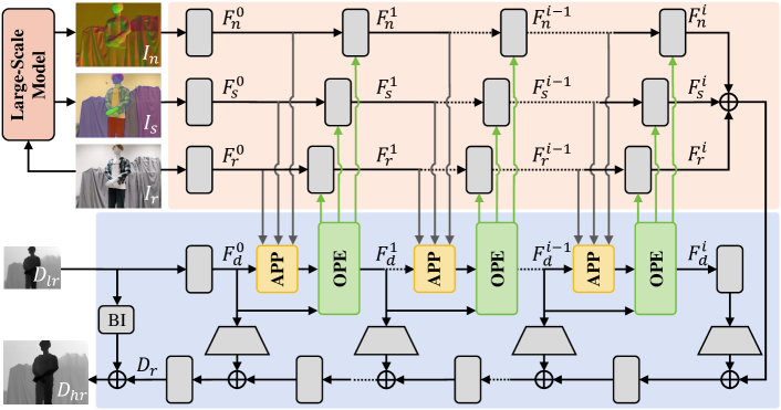
A naive guided DSR architecture typically incorporates an RGB guidance branch and a depth recovery branch. As such, we introduce additional normal and semantic guidance branches, collectively forming the scene prior branch. Subsequently, in the depth recovery branch, the HR depth is progressively restored through multiple stages, under the guidance of the scene prior branch.

Let $\boldsymbol{I}_{r}\in R^{sh\times sw\times 3}$, $\boldsymbol{D}_{lr}\in R^{h\times w\times 1}$, and $\boldsymbol{D}_{hr}\in R^{sh\times sw\times 1}$ denote the RGB, LR depth, and predicted HR depth, respectively, where $h$ and $w$ are the height and width of LR depth, and $s$ is the upsampling factor (e.g., 4, 8, 16). Similar to the existing methods [26, 33], we exploit residual groups [46] $f_{rg}$ as the basic feature learning unit (gray rectangles in Figs. 2-4). Fig. 2 shows the overall architecture of SPFNet, consisting of a scene prior branch (orange part) and a depth branch (blue part). Given $I_{r}$, we generate both normal $\boldsymbol{I}_{n}\in R^{sh\times sw\times 3}$ and semantic $\boldsymbol{I}_{s}\in R^{sh\times sw\times 1}$ priors using large-scale models, i.e., Omnidata [6] and SAM [16].

In the scene prior branch, $\boldsymbol{I}_{r}$, $\boldsymbol{I}_{s}$, and $\boldsymbol{I}_{n}$ are first fed into $f_{rg}$, yielding prior features $\boldsymbol{F}_{r}^{0}$, $\boldsymbol{F}_{s}^{0}$, and $\boldsymbol{F}_{n}^{0}$, all of which serve as the input of the first APP module. Meanwhile, we conduct $f_{rg}$ to fuse $\boldsymbol{F}_{r}^{0}$, $\boldsymbol{F}_{s}^{0}$, and $\boldsymbol{F}_{n}^{0}$ and the output features of OPE, obtaining $\boldsymbol{F}_{r}^{1}$, $\boldsymbol{F}_{s}^{1}$, and $\boldsymbol{F}_{n}^{1}$, respectively. The three features are then fed into the second APP. The remaining portion continues to perform the same action until it obtains $\boldsymbol{F}_{r}^{i}$, $\boldsymbol{F}_{s}^{i}$, and $\boldsymbol{F}_{n}^{i}$, which are merged into the depth branch.

In the depth recovery branch, $\boldsymbol{D}_{lr}$ is first input into $f_{rg}$, obtaining the depth prior feature $\boldsymbol{F}_{d}^{0}$. APP encodes it along with $\boldsymbol{F}_{r}^{0}$, $\boldsymbol{F}_{s}^{0}$, and $\boldsymbol{F}_{n}^{0}$ to calculate the similarity weight and enhanced depth prior feature. Then, OPE takes as input the feature, weight, and $\boldsymbol{F}_{d}^{0}$, producing $\boldsymbol{F}_{d}^{1}$. Next, we recursively conduct APP and OPE to refine the depth features, yielding $\boldsymbol{F}_{d}^{i}$.

Among the $i$ stages, the historical depth feature $\boldsymbol{F}_{d}^{i}$ and the scene prior features $\boldsymbol{F}_{n}^{i}$, $\boldsymbol{F}_{s}^{i}$, and $\boldsymbol{F}_{r}^{i}$ are aggregated to reconstruct the depth $\boldsymbol{D}_{r}$. Finally, the predicted HR depth $\boldsymbol{D}_{hr}$ is formulated as:

$$\boldsymbol{D}_{hr}=\boldsymbol{D}_{r}+f_{bi}(\boldsymbol{D}_{lr}),$$ (1)

where $f_{bi}$ refers to bicubic interpolation function.

To strike a balance between model complexity and performance, we propose a lightweight model, SPFNet-T. This is achieved by reducing the number of channels in all convolutions while keeping the network architecture unchanged.

Figure 3: Scheme of (a) All-in-one Prior Propagation (APP), and (b) histogram comparison of scene prior features before and after APP.

3.2 All-in-one Prior Propagation

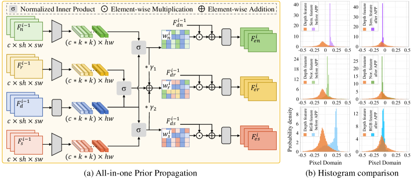
The proposed APP module weakens the texture interference by using the inherent characteristics of scene priors from large-scale models. It computes the similarity between the multi-modal scene priors (RGB, normal, semantic, and depth), which is then used to mitigate the interference and promote the generation of scene prior filter kernels. As shown in Fig. 3(a), we first downsample prior features $\boldsymbol{F}_{n}^{i-1}$, $\boldsymbol{F}_{r}^{i-1}$, and $\boldsymbol{F}_{s}^{i-1}$ to match the size of the depth feature $\boldsymbol{F}_{d}^{i-1}$. Next, APP unfolds (by $3\times 3$ kernel) them into patches together with $\boldsymbol{F}_{d}^{i-1}$, denoted as $n_{j}^{i-1}$, $r_{j}^{i-1}$, $s_{j}^{i-1}$, and $d_{j}^{i-1}$, where $j\in[1,h\times w]$. Similar to the existing methods [40, 21, 53], we compute the patch similarity $\sigma_{j}^{p}$ between the $j$-th prior patch $p_{j}^{i-1}$ (e.g., $r_{j}^{i-1}$, $n_{j}^{i-1}$, $s_{j}^{i-1}$) and depth patch $d_{j}^{i-1}$ using normalized inner product:

$$\sigma_{j}^{p}=\left\langle\frac{p_{j}^{i-1}}{\left\|p_{j}^{i-1}\right\|},\frac{d_{j}^{i-1}}{\left\|d_{j}^{i-1}\right\|}\right\rangle.$$ (2)

The overall similarity between the scene prior and depth features can be derived by calculating the $\sigma_{j}^{p}$ of all patches, generating surface normal $\boldsymbol{w}_{n}^{i}$, semantic $\boldsymbol{w}_{s}^{i}$, and RGB $\boldsymbol{w}_{r}^{i}$ weights:

$$\boldsymbol{w}_{r}^{i}=\gamma_{1}\ast\boldsymbol{w}_{n}^{i}+\gamma_{2}\ast\boldsymbol{w}_{s}^{i}+\mathcal{F}(\mathcal{C}_{j=1}^{h\times w}\sigma_{j}^{r}),$$ (3)

where $\boldsymbol{w}_{n}^{i}=\mathcal{F}(\mathcal{C}_{j=1}^{h\times w}\sigma_{j}^{n})$ and $\boldsymbol{w}_{s}^{i}=\mathcal{F}(\mathcal{C}_{j=1}^{h\times w}\sigma_{j}^{s})$. $\mathcal{C}$ and $\mathcal{F}$ denote concatenation and fold, respectively. $\gamma_{1}$ and $\gamma_{2}$ are learnable parameters.

Finally, the APP utilizes the similarity weights to attenuate interference:

$$\begin{split}&\boldsymbol{F}_{en}^{i}=f_{rg}\left(\boldsymbol{F}_{dn}^{i-1}\odot\boldsymbol{w}_{n}^{i}+\boldsymbol{F}_{dn}^{i-1}\right),\\ &\boldsymbol{F}_{er}^{i}=f_{rg}\left(\boldsymbol{F}_{dr}^{i-1}\odot\boldsymbol{w}_{r}^{i}+\boldsymbol{F}_{dr}^{i-1}\right),\\ &\boldsymbol{F}_{es}^{i}=f_{rg}\left(\boldsymbol{F}_{ds}^{i-1}\odot\boldsymbol{w}_{s}^{i}+\boldsymbol{F}_{ds}^{i-1}\right),\end{split}$$ (4)

where $\boldsymbol{F}_{en}^{i}$, $\boldsymbol{F}_{er}^{i}$, and $\boldsymbol{F}_{es}^{i}$ respectively indicate the normal, RGB, and semantic features enhanced by the APP. $\odot$ is element-wise multiplication. Fig. 3(b) illustrates the histogram of prior features. It can be found that the output prior features of the APP are closer to the distribution of depth features, demonstrating that our APP succeeds calibrating prior features and reducing interference.

3.3 One-to-One Prior Embedding

The OPE module continuously integrates each single-modal prior (normal, semantic, and RGB) into depth to further reduce interference and enhance edges. Fig. 4(a) shows the main steps of the OPE module. First, given the enhanced scene prior features ($\boldsymbol{F}_{en}^{i}$, $\boldsymbol{F}_{er}^{i}$, $\boldsymbol{F}_{es}^{i}$), similarity weights ($\boldsymbol{w}_{n}^{i}$, $\boldsymbol{w}_{r}^{i}$, $\boldsymbol{w}_{s}^{i}$), and depth features $\boldsymbol{F}_{d}^{i-1}$, OPE conducts MGF, denoted as $f_{m}$, to successively embed each single-modal prior into depth:

$$\begin{split}&\boldsymbol{F}_{dn}^{i},\boldsymbol{F}_{nd}^{i}=f_{m}\left(f_{c}\left(\boldsymbol{F}_{d}^{i-1}\right),\boldsymbol{F}_{en}^{i},\boldsymbol{w}_{n}^{i}\right),\\ &\boldsymbol{F}_{ds}^{i},\boldsymbol{F}_{sd}^{i}=f_{m}\left(f_{c}\left(\boldsymbol{F}_{d}^{i-1}+\boldsymbol{F}_{nd}^{i}\right),\boldsymbol{F}_{es}^{i},\boldsymbol{w}_{s}^{i}\right),\\ &\boldsymbol{F}_{dr}^{i},\boldsymbol{F}_{rd}^{i}=f_{m}\left(f_{c}\left(\boldsymbol{F}_{nd}^{i}+\boldsymbol{F}_{sd}^{i}\right),\boldsymbol{F}_{er}^{i},\boldsymbol{w}_{r}^{i}\right),\end{split}$$ (5)

where $\boldsymbol{F}_{dn}^{i}$, $\boldsymbol{F}_{ds}^{i}$, and $\boldsymbol{F}_{dr}^{i}$ indicate the filtered normal, semantic, and RGB features, respectively. In addition, $\boldsymbol{F}_{nd}^{i}$, $\boldsymbol{F}_{sd}^{i}$, and $\boldsymbol{F}_{rd}^{i}$ correspond to the filtered depth features of normal-to-depth, semantic-to-depth, and RGB-to-depth, severally. $f_{c}$ is convolutional layer. Then, OPE aggregates the filtered scene prior and depth features, yielding the enhanced depth feature $\boldsymbol{F}_{d}^{i}$:

$$\boldsymbol{F}_{d}^{i}=f_{rg}(\mathcal{C}(\boldsymbol{F}_{dn}^{i},\boldsymbol{F}_{ds}^{i},\boldsymbol{F}_{dr}^{i},\boldsymbol{F}_{fd}^{i}))+\boldsymbol{F}_{d}^{i-1},$$ (6)

where $\boldsymbol{F}_{fd}^{i}=f_{c}(\mathcal{C}(\boldsymbol{F}_{nd}^{i},\boldsymbol{F}_{sd}^{i},\boldsymbol{F}_{rd}^{i}))+\boldsymbol{F}_{d}^{i-1}$, and $\mathcal{C}$ refers to concatenation.

Figure 4: Scheme of (a) One-to-one Prior Embedding (OPE), and (b) gradient histogram of filter kernels in the texture area (green box). The surface normal, semantic, and RGB kernels are generated by our Mutual Guided Filtering (MGF).

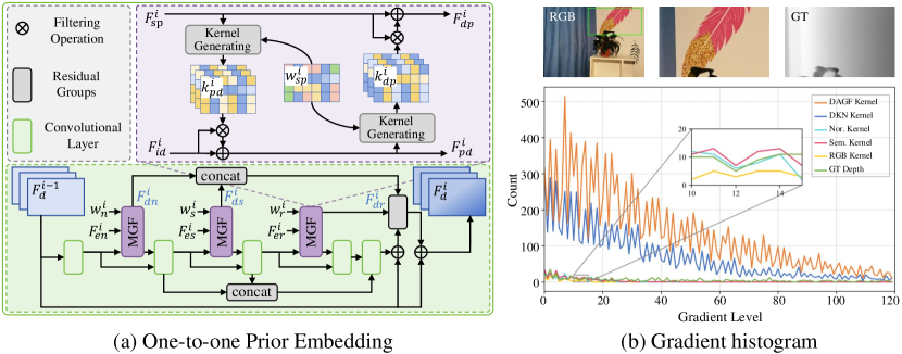
Mutual Guided Filter. In contrast to existing guided filtering methods [14, 5, 51, 45], our MGF emphasizes on employing scene priors and similarity weights to reduce texture interference within the filter kernel and enhance the accuracy of the edges. As depicted in the purple part of Fig. 4(a), it includes both prior-to-depth filtering and depth-to-prior filtering.

For prior-to-depth filtering, MGF first takes scene prior features $\boldsymbol{F}_{sp}^{i}$ (e.g., $\boldsymbol{F}_{en}^{i}$, $\boldsymbol{F}_{er}^{i}$, $\boldsymbol{F}_{es}^{i}$), similarity weights $\boldsymbol{w}_{sp}^{i}$ (e.g., $\boldsymbol{w}_{n}^{i}$, $\boldsymbol{w}_{r}^{i}$, $\boldsymbol{w}_{s}^{i}$) and depth features $\boldsymbol{F}_{id}^{i}$ as inputs. It then constructs scene prior filter kernels, denoted as $\boldsymbol{k}_{pd}^{i}$. These kernels are subsequently applied to filter the depth features $\boldsymbol{F}_{id}^{i}$, thereby enabling the transfer of high-frequency components from the scene priors to the depth. The filtered depth features $\boldsymbol{F}_{pd}^{i}$ is described as:

$$\boldsymbol{F}_{pd}^{i}=\boldsymbol{F}_{id}^{i}\otimes\boldsymbol{k}_{pd}^{i}+\boldsymbol{F}_{id}^{i},$$ (7)

where $\boldsymbol{k}_{pd}^{i}=f_{kg}\left(\boldsymbol{F}_{sp}^{i},\boldsymbol{w}_{sp}^{i}\right)$. $f_{kg}$ stands for kernel generating module, consisting of a $1\times 1$ convolution and an activation function. $\otimes$ is the filtering operation.

Similarly, for depth-to-prior filtering, $\boldsymbol{w}_{sp}^{i}$ and the filtered depth feature $\boldsymbol{F}_{pd}^{i}$ are first fed into $f_{kg}$, generating the depth filter kernel $\boldsymbol{k}_{dp}^{i}$. Then, MGF filters prior features $\boldsymbol{F}_{sp}^{i}$ to preserve the structure required for the depth and further attenuate interference. The filtered prior features $\boldsymbol{F}_{dp}^{i}$ is defined as:

$$\boldsymbol{F}_{dp}^{i}=\boldsymbol{F}_{sp}^{i}\otimes\boldsymbol{k}_{dp}^{i}+\boldsymbol{F}_{sp}^{i}.$$ (8)

where $\boldsymbol{k}_{dp}^{i}=f_{kg}\left(\boldsymbol{F}_{pd}^{i},\boldsymbol{w}_{sp}^{i}\right)$. Fig. 4(b) shows the gradient histogram of filter kernels. Notably, our surface normal, semantic, and RGB kernels exhibit less gradient variations and are closer to GT depth than DKN [14] and DAGF [51]. These results further validate that MGF can efficiently mitigate the interference.

3.4 Loss Function

We optimize our SPFNet by minimizing the $L_{1}$ loss between the predicted depth $\boldsymbol{D}_{hr}$ and ground truth depth $\boldsymbol{D}_{gt}$:

$$\mathcal{L}_{total}=\sum_{q\in Q}\left\|\boldsymbol{D}_{gt}^{q}-\boldsymbol{D}_{hr}^{q}\right\|_{1},$$ (9)

where Q is the set of valid pixels of $\boldsymbol{D}_{gt}$. $\left\|\cdot\right\|_{1}$ denotes $L_{1}$ norm.

4 Experimental Results

4.1 Experimental Setups and Implementation Details

We carry out extensive experiments on four DSR benchmarks, including both synthetic NYU-v2 [27], Lu [22], Middlebury [11, 25] and real-world RGB-D-D [10] datasets. For synthetic scenarios, similar to [14, 49, 33, 48], the LR depth is produced by downsampling the ground truth depth using bicubic interpolation. As a result, our model is trained on the 1,000 RGB-D pairs of NYU-v2, with the remaining 449 pairs for testing. In addition, the pre-trained model on NYU-v2 is further evaluated on Lu (6 pairs), Middlebury (30 pairs), and RGB-D-D (405 pairs) test sets. To evaluate the performance in real-world environments, we train our SPFNet on RGB-D-D, which consists of 2,215 RGB-D pairs for training and 405 pairs for testing, where LR depth and ground truth depth are captured by Huawei P30 Pro and the Lucid Helios, respectively.

We utilize the Root Mean Square Error (RMSE) metric in centimeters to evaluate the DSR methods [14, 26, 43, 48]. During training, the scene priors and GT depth are cropped to $256\times 256$. We employ the Adam [15] optimizer with an initial learning rate of $1\times 10^{-4}$ to train our SPFNet. The proposed model is implemented using PyTorch with a single NVIDIA GeForce RXT 4090.

4.2 Comparison with the State-of-the-Art

We compare SPFNet with state-of-the-art methods on $\times 4$, $\times 8$, and $\times 16$ DSR, including DSRNet [8], DJF [19], DJFR [20], PAC [29], CUNet [4], DKN [14], FDKN [14], FDSR [10], DAGF [51], DCTNet [49], GraphSR [3], SUFT [10], RSAG [42], DADA [23], SSDNet [48], and SGNet [33].

Table 1: Quantitative comparison with state-of-the-art methods on four benchmarks, with scale factors $\times 4$, $\times 8$, and $\times 16$. *P refers to parameters.

Methods	*P (M)	NYU-v2			RGB-D-D			Lu			Middlebury
		$\times$4	$\times$8	$\times$16	$\times$4	$\times$8	$\times$16	$\times$4	$\times$8	$\times$16	$\times$4	$\times$8	$\times$16
DJF [19]	$<1.2$	2.80	5.33	9.46	3.41	5.57	8.15	1.65	3.96	6.75	1.68	3.24	5.62
DJFR [20]		2.38	4.94	9.18	3.35	5.57	7.99	1.15	3.57	6.77	1.32	3.19	5.57
PAC [29]		1.89	3.33	6.78	1.25	1.98	3.49	1.20	2.33	5.19	1.32	2.62	4.58
CUNet [4]		1.92	3.70	6.78	1.18	1.95	3.45	0.91	2.23	4.99	1.10	2.17	4.33
DKN [14]		1.62	3.26	6.51	1.30	1.96	3.42	0.96	2.16	5.11	1.23	2.12	4.24
FDKN [14]		1.86	3.58	6.96	1.18	1.91	3.41	0.82	2.10	5.05	1.08	2.17	4.50
FDSR [10]		1.61	3.18	5.86	1.16	1.82	3.06	1.29	2.19	5.00	1.13	2.08	4.39
DCTNet [49]		1.59	3.16	5.84	1.08	1.74	3.05	0.88	1.85	4.39	1.10	2.05	4.19
SSDNet [48]		1.60	3.14	5.86	1.04	1.72	2.92	0.80	1.82	4.77	1.02	1.91	4.02
SPFNet-T		1.52	3.03	5.71	1.16	1.77	2.90	0.80	1.69	4.31	1.04	1.78	3.40
DSRNet [8]	$>30$	3.00	5.16	8.41	-	-	-	1.77	3.10	5.11	1.77	3.05	4.96
GraphSR [3]		1.79	3.17	6.02	1.30	1.83	3.12	0.92	2.05	5.15	1.11	2.12	4.43
SUFT [26]		1.12	2.51	4.86	1.10	1.69	2.71	1.10	1.74	3.92	1.07	1.75	3.18
RSAG [42]		1.23	2.51	5.27	1.14	1.75	2.96	0.79	1.67	4.30	1.13	2.74	3.55
DADA [23]		1.54	2.74	4.80	1.20	1.83	2.80	0.96	1.87	4.01	1.20	2.03	4.18
SGNet [33]		1.10	2.44	4.77	1.10	1.64	2.55	1.03	1.61	3.55	1.15	1.64	2.95
SPFNet		1.09	2.36	4.55	1.13	1.70	2.53	0.90	1.56	3.20	1.05	1.58	2.85

Figure 5: Complexity on NYU-v2 dataset ($\times 16$) with parameters $<1.2M$ (left) and parameters $>30M$ (right), tested by a 4090 GPU. Circle area indicates inference time.

Table 2: Quantitative comparison on real-world RGB-D-D dataset.

Train	FDSR [10]	DCTNet [49]	SUFT [26]	SSDNet [48]	SGNet [33]	SPFNet-T	SPFNet
NYU-v2	7.50	7.37	7.22	7.32	7.22	7.21	7.23
RGB-D-D	5.49	5.43	5.41	5.38	5.32	4.63	4.18

Figure 6: Visual results and error maps on NYU-v2 dataset ($\times 16$).

Figure 7: Visual results and error maps on RGB-D-D dataset ($\times 16$).

Figure 8: Visual results and error maps on Lu dataset ($\times 16$).

Figure 9: Visual results and error maps on Middlebury dataset ($\times 16$).

Figure 10: Visual results on real-world RGB-D-D dataset.

Quantitative Comparison. Tabs. 1 and 2 demonstrate that both our SPFNet and SPFNet-T achieve state-of-the-art performance on both the synthetic and real-world datasets, respectively. In detail, Tab. 1 enumerates the quantitative comparison on four datasets, with scale factors of $\times 4$, $\times 8$, and $\times 16$. For parameters fewer than $1.2M$, we discover that our SPFNet-T outperforms most other methods. For example, our SPFNet-T reduces the RMSE by $0.62cm$ (Middlebury) and $0.46cm$ (Lu) on $\times 16$ DSR, compared to the second best method. For parameters exceeding $30M$, we observe that our SPFNet is also surpasses others. For instance, our SPFNet decreases the RMSE by $0.22cm$ (NYU-v2) and $0.35cm$ (Lu), compared to the suboptimal method on $\times 16$ DSR.

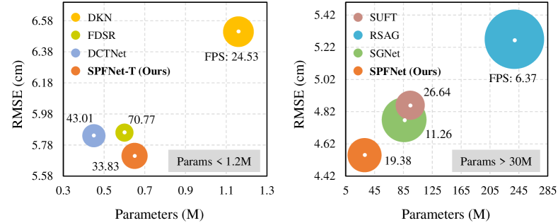
Fig. 5 shows that our model achieves an excellent balance between parameters, inference time, FPS, and performance. Notably, for parameters below $1.2M$, SPFNet-T significantly reduces RMSE with a minimal increase in parameters and inference time. For parameters exceeding $30M$, SPFNet markedly enhances performance while decreasing parameters. For example, SPFNet outperforms SUFT by reducing $66.26M$ parameters and $0.22cm$ RMSE, with a slight $17ms$ increase in inference time. Overall, our method effectively balances RMSE and complexity, resulting in a considerable performance improvement.

Tab. 2 reports the results on the real-world RGB-D-D dataset. Similar to the existing methods [10, 49, 33], we first use the model pre-trained on NYU-v2 to predict the real-world RGB-D-D depth without fine-tuning, resulting in the first row of Tab. 2. Then, we retrain and test on the real-world RGB-D-D dataset, yielding the second row. It is evident that our method is superior to others. For example, SPFNet is $1.14cm$ lower compared to the SGNet. These results suggest that our method effectively improves the performance of DSR.

Table 3: Results of joint DSR and denoising on NYU-v2 and Middlebury datasets.

Scale	DJF [19]	DJFR [20]	DSRNet [8]	PAC [29]	DKN [14]	DAGF [51]	SPFNet-T	SPFNet
NYU-v2
$\times 4$	3.74	4.01	4.36	4.23	3.39	3.25	3.45	2.94
$\times 8$	5.95	6.21	6.31	6.24	5.24	5.01	5.15	4.66
$\times 16$	9.61	9.90	9.75	9.54	8.41	7.54	7.94	6.96
Middlebury
$\times 4$	1.80	1.86	1.84	1.81	1.76	1.72	1.67	1.66
$\times 8$	2.99	3.07	2.99	2.94	2.68	2.61	2.61	2.43
$\times 16$	5.16	5.27	4.70	5.08	4.55	4.24	4.24	3.86

Figure 11: Visual results of joint DSR and denoising on NYU-v2 and Middlebury ($\times 16$).

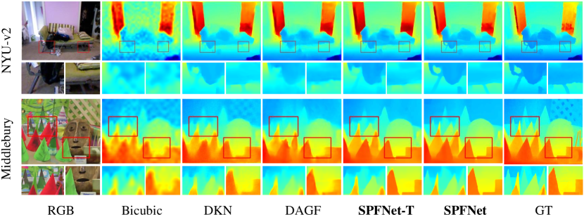
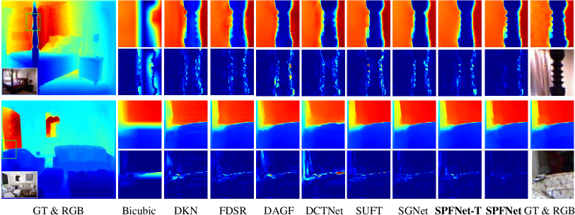
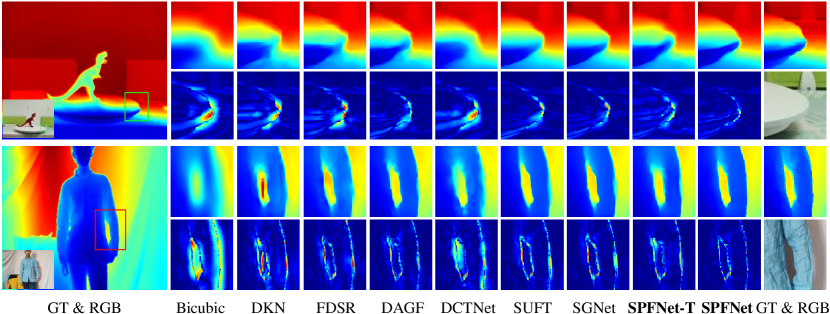
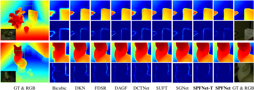
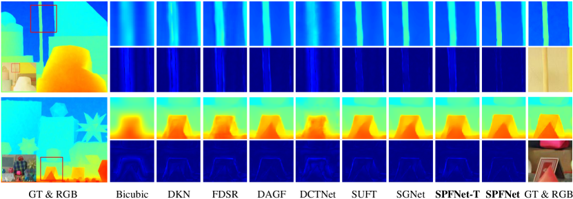
Visual Comparison. Figs. 6-10 provide visual comparison results on both the synthetic (Figs. 6-9) and real-world (Fig. 10) datasets. In the error maps, a brighter color indicates a larger error. It is evident that our method predicts depth with superior edge accuracy and fewer errors. For example, the edges of the person’s arm in Fig. 7 and the sculpture in Fig. 8 are more distinct compared to other methods, while the error maps display smaller errors.

Different from synthetic datasets, LR depth captured in real-world environment often exhibits severe structure distortion. Fig. 10 shows the visual results on the real-world RGB-D-D dataset, demonstrating that our approach is capable of recovering more accurate edges compared to other methods. For instance, the edges of the hand and the box predicted by our SPFNet in Fig. 10 are more closely aligned with the ground-truth depth. In short, these visual results confirm that our method is very effective in restoring HR depth.

Joint DSR and Denoising. Tabs. 3 demonstrates that our method outperforms other methods in joint DSR and denoising on NYU-v2 and Middlebury datasets. Depth obtained in real environment is often noisy, which poses a challenge to the HR depth restoration. Similar to the existing method [51], we add Gaussian noise with a variance of $25$ to the LR depth as input. As evidenced by Tab. 3, compared to the second-best method, our SPFNet reduces the RMSE by $0.35cm$ ($\times 8$) and $0.58cm$ ($\times 16$) on the NYU-v2 dataset, and by $0.18cm$ ($\times 8$) and $0.38cm$ ($\times 16$) on the Middlebury dataset. Furthermore, Fig. 11 presents the visual comparison on NYU-v2 and Middlebury datasets. Notably, the depth edges predicted by our SPFNet are more accurate. For example, the edges of the bed legs in Fig. 11 (NYU-v2) are clearer than other approaches. These results confirm that our SPFNet exhibits superior performance and generalization.

Figure 12: Ablation study of surface normal and semantic on $\times 16$ DSR.

Figure 13: Ablation study of APP and OPE. The ‘S+R+N’ refers to the filter in the order of semantic (S), RGB (R), and surface normal (N).

4.3 Ablation Study

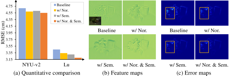
Surface Normal and Semantic priors. Fig. 12 shows the ablation study of surface normal and semantic priors. For the baseline, similar to the existing method [10, 49, 33], only RGB is utilized as guidance. From Fig. 12(a), we find that both surface normal and semantic priors contribute to a decrease in RMSE. When both are employed together, SPFNet achieves the best performance. For example, compared to the baseline, surface normal and semantic priors reduce the RMSE by $0.11cm$ and $0.15cm$ on the Lu dataset, respectively. Finally, our SPFNet outperforms the baseline by $0.25cm$ on the Lu dataset.

Fig. 12(b) and (c) illustrate the visual results of depth feature and error maps. We observe that both surface normal and semantic priors are capable of producing more distinctive edges and fewer errors than the baseline. Furthermore, when combining them, our SPFNet generates the much clearer structure and the much lesser errors. These results suggest that, by leveraging scene priors, our SPFNet can effectively enhance depth edges and minimize errors.

APP and OPE. Fig. 13(a) presents the ablation study of APP and OPE. The baseline (blue dotted line) removes all APP and OPE from SPFNet. It can be discovered that both APP and OPE contribute to performance improvement. When they are utilized in conjunction, our method (solid orange line) achieves the best performance. For instance, our SPFNet surpasses the baseline by $0.3cm$ on the NYU-v2 dataset and $0.33cm$ on the Lu dataset, respectively.

In addition, Fig. 13(b) shows the ablation study of different iterations of APP and OPE. It is evident that the performance incrementally improves as the number of APP and OPE increases. When APP & OPE-4 is utilized, the RMSE consistently reduces on NYU and Lu datasets, but only slightly on Middlebury and RGB-D-D datasets. To better balance model complexity and performance, we select APP & OPE-3 (solid orange line) as the setting for our SPFNet.

Finally, Fig. 13(c) depicts the ablation study of single-modal prior filter order in OPE, performed on the NYU-v2 and Middlebury datasets. It is clearly discernible that the order of ‘N+S+R’ (orange bars) achieves the lowest RMSE.

Table 4: Ablation on MGF. D2P: depth-to-prior filtering, P2D: prior-to-depth filtering. D2P$\rightarrow$P2D means that the D2P step precedes the P2D step.

Method	D2P	P2D	D2P$\rightarrow$P2D	P2D$\rightarrow$D2P	Similarity	Params (M)	NYU-v2	Lu
(a)						29.76 $(\pm 0.00)$	2.59 $(\pm 0.00)$	1.75 $(\pm 0.00)$
(b)	✓					30.22 $(+0.46)$	2.51 $(-0.08)$	1.70 $(-0.05)$
(c)		✓				30.22 $(+0.46)$	2.48 $(-0.11)$	1.64 $(-0.11)$
(d)	✓	✓	✓			30.68 $(+0.92)$	2.46 $(-0.13)$	1.61 $(-0.14)$
(e)	✓	✓		✓		30.68 $(+0.92)$	2.40 $(-0.19)$	1.59 $(-0.16)$
(f)	✓	✓		✓	✓	30.68 $(+0.92)$	2.36 $(-0.23)$	1.56 $(-0.19)$

MGF. Tab. 4 reports the ablation study of MGF on $\times 8$ DSR. For the baseline (a), we remove all guided image filtering in SPFNet. (b) and (c) employ solely depth-to-prior filtering (D2P) or prior-to-depth filtering (P2D), respectively, both of which enhance DSR performance compared to (a). (d) and (e) explore different combination orders of D2P and P2D. It can be found that both (d) and (e) achieve lower RMSE than (a)-(d). Based on (e), (f) further leverages the similarity weights to guide the generation of the filter kernel, contributing to the best performance, i.e., surpassing the baseline (a) by $0.23cm$ on NYU-v2 dataset and $0.19cm$ on Lu dataset, respectively.

5 Conclusion

In this paper, we propose SPFNet, a novel DSR solution that utilizes the surface normal and semantic priors from large-scale models to effectively weaken the texture interference and improve the edge accuracy. Specifically, we design the all-in-one prior propagation that mitigates interference by calculating the similarity weights between multi-modal scene priors. Moreover, we develop the one-to-one prior embedding that continuously aggregates each single-modal prior into the depth using mutual guidance filtering, further reducing interference and enhancing edge. Comprehensive experiments on four benchmarks demonstrate that our SPFNet performs favorably against state-of-the-art approaches.

6 Limitation

Apart from using the predicted results of those large-scale models, a prevalent alternative is to transfer their pre-trained knowledge into depth map super-resolution models. Thus, in future research, we aim to explore the prompting learning to further minimize the texture interference and improve edge accuracy.

References

- [1] Caesar, H., Bankiti, V., Lang, A.H., Vora, S., Liong, V.E., Xu, Q., Krishnan, A., Pan, Y., Baldan, G., Beijbom, O.: nuscenes: A multimodal dataset for autonomous driving. In: CVPR. pp. 11621–11631 (2020)
- [2] Chen, Y., Fan, H., Xu, B., Yan, Z., Kalantidis, Y., Rohrbach, M., Yan, S., Feng, J.: Drop an octave: Reducing spatial redundancy in convolutional neural networks with octave convolution. In: ICCV. pp. 3435–3444 (2019)
- [3] De Lutio, R., Becker, A., D’Aronco, S., Russo, S., Wegner, J.D., Schindler, K.: Learning graph regularisation for guided super-resolution. In: CVPR. pp. 1979–1988 (2022)
- [4] Deng, X., Dragotti, P.L.: Deep convolutional neural network for multi-modal image restoration and fusion. IEEE transactions on pattern analysis and machine intelligence 43(10), 3333–3348 (2020)
- [5] Dong, X., Yokoya, N., Wang, L., Uezato, T.: Learning mutual modulation for self-supervised cross-modal super-resolution. In: ECCV. pp. 1–18. Springer (2022)
- [6] Eftekhar, A., Sax, A., Malik, J., Zamir, A.: Omnidata: A scalable pipeline for making multi-task mid-level vision datasets from 3d scans. In: ICCV. pp. 10786–10796 (2021)
- [7] Fan, R., Wang, H., Cai, P., Liu, M.: Sne-roadseg: Incorporating surface normal information into semantic segmentation for accurate freespace detection. In: ECCV. pp. 340–356. Springer (2020)
- [8] Guo, C., Li, C., Guo, J., Cong, R., Fu, H., Han, P.: Hierarchical features driven residual learning for depth map super-resolution. IEEE Transactions on Image Processing 28(5), 2545–2557 (2018)
- [9] He, K., Sun, J., Tang, X.: Guided image filtering. IEEE transactions on pattern analysis and machine intelligence 35(6), 1397–1409 (2012)
- [10] He, L., Zhu, H., Li, F., Bai, H., Cong, R., Zhang, C., Lin, C., Liu, M., Zhao, Y.: Towards fast and accurate real-world depth super-resolution: Benchmark dataset and baseline. In: CVPR. pp. 9229–9238 (2021)
- [11] Hirschmuller, H., Scharstein, D.: Evaluation of cost functions for stereo matching. In: CVPR. pp. 1–8 (2007)
- [12] Hui, T.W., Loy, C.C., Tang, X.: Depth map super-resolution by deep multi-scale guidance. In: ECCV. pp. 353–369. Springer (2016)
- [13] Im, S., Ha, H., Choe, G., Jeon, H.G., Joo, K., Kweon, I.S.: Accurate 3d reconstruction from small motion clip for rolling shutter cameras. IEEE transactions on pattern analysis and machine intelligence 41(4), 775–787 (2018)
- [14] Kim, B., Ponce, J., Ham, B.: Deformable kernel networks for joint image filtering. International Journal of Computer Vision 129(2), 579–600 (2021)
- [15] Kingma, D.P., Ba, J.: Adam: A method for stochastic optimization. arXiv preprint arXiv:1412.6980 (2014)
- [16] Kirillov, A., Mintun, E., Ravi, N., Mao, H., Rolland, C., Gustafson, L., Xiao, T., Whitehead, S., Berg, A.C., Lo, W.Y., et al.: Segment anything. arXiv preprint arXiv:2304.02643 (2023)
- [17] Li, L., Li, X., Yang, S., Ding, S., Jolfaei, A., Zheng, X.: Unsupervised-learning-based continuous depth and motion estimation with monocular endoscopy for virtual reality minimally invasive surgery. IEEE Transactions on Industrial Informatics 17(6), 3920–3928 (2020)
- [18] Li, X., Chen, C., Zhou, S., Lin, X., Zuo, W., Zhang, L.: Blind face restoration via deep multi-scale component dictionaries. In: ECCV. pp. 399–415. Springer (2020)
- [19] Li, Y., Huang, J.B., Ahuja, N., Yang, M.H.: Deep joint image filtering. In: ECCV. pp. 154–169. Springer (2016)
- [20] Li, Y., Huang, J.B., Ahuja, N., Yang, M.H.: Joint image filtering with deep convolutional networks. IEEE transactions on pattern analysis and machine intelligence 41(8), 1909–1923 (2019)
- [21] Lu, L., Li, W., Tao, X., Lu, J., Jia, J.: Masa-sr: Matching acceleration and spatial adaptation for reference-based image super-resolution. In: CVPR. pp. 6368–6377 (2021)
- [22] Lu, S., Ren, X., Liu, F.: Depth enhancement via low-rank matrix completion. In: CVPR. pp. 3390–3397 (2014)
- [23] Metzger, N., Daudt, R.C., Schindler, K.: Guided depth super-resolution by deep anisotropic diffusion. In: CVPR. pp. 18237–18246 (2023)
- [24] Qiu, J., Cui, Z., Zhang, Y., Zhang, X., Liu, S., Zeng, B., Pollefeys, M.: Deeplidar: Deep surface normal guided depth prediction for outdoor scene from sparse lidar data and single color image. In: CVPR. pp. 3313–3322 (2019)
- [25] Scharstein, D., Pal, C.: Learning conditional random fields for stereo. In: CVPR. pp. 1–8 (2007)
- [26] Shi, W., Ye, M., Du, B.: Symmetric uncertainty-aware feature transmission for depth super-resolution. In: ACMMM. pp. 3867–3876 (2022)
- [27] Silberman, N., Hoiem, D., Kohli, P., Fergus, R.: Indoor segmentation and support inference from rgbd images. In: ECCV. pp. 746–760. Springer (2012)
- [28] Song, X., Dai, Y., Zhou, D., Liu, L., Li, W., Li, H., Yang, R.: Channel attention based iterative residual learning for depth map super-resolution. In: CVPR. pp. 5631–5640 (2020)
- [29] Su, H., Jampani, V., Sun, D., Gallo, O., Learned-Miller, E., Kautz, J.: Pixel-adaptive convolutional neural networks. In: CVPR. pp. 11166–11175 (2019)
- [30] Sun, B., Ye, X., Li, B., Li, H., Wang, Z., Xu, R.: Learning scene structure guidance via cross-task knowledge transfer for single depth super-resolution. In: CVPR. pp. 7792–7801 (2021)
- [31] Tang, Q., Cong, R., Sheng, R., He, L., Zhang, D., Zhao, Y., Kwong, S.: Bridgenet: A joint learning network of depth map super-resolution and monocular depth estimation. In: ACMMM. pp. 2148–2157 (2021)
- [32] Wang, K., Zhao, L., Zhang, J., Zhang, J., Wang, A., Bai, H.: Joint depth map super-resolution method via deep hybrid-cross guidance filter. Pattern Recognition 136, 109260 (2023)
- [33] Wang, Z., Yan, Z., Yang, J.: Sgnet: Structure guided network via gradient-frequency awareness for depth map super-resolution. arXiv preprint arXiv:2312.05799 (2023)
- [34] Wu, Y., Pan, C., Wang, G., Yang, Y., Wei, J., Li, C., Shen, H.T.: Learning semantic-aware knowledge guidance for low-light image enhancement. In: CVPR. pp. 1662–1671 (2023)
- [35] Xu, Y., Zhu, X., Shi, J., Zhang, G., Bao, H., Li, H.: Depth completion from sparse lidar data with depth-normal constraints. In: ICCV. pp. 2811–2820 (2019)
- [36] Yan, Z., Li, X., Wang, K., Chen, S., Li, J., Yang, J.: Distortion and uncertainty aware loss for panoramic depth completion. In: ICML. pp. 39099–39109. PMLR (2023)
- [37] Yan, Z., Wang, K., Li, X., Zhang, Z., Li, G., Li, J., Yang, J.: Learning complementary correlations for depth super-resolution with incomplete data in real world. IEEE transactions on neural networks and learning systems (2022)
- [38] Yan, Z., Wang, K., Li, X., Zhang, Z., Li, J., Yang, J.: Rignet: Repetitive image guided network for depth completion. In: ECCV. pp. 214–230. Springer (2022)
- [39] Yan, Z., Wang, K., Li, X., Zhang, Z., Li, J., Yang, J.: Desnet: Decomposed scale-consistent network for unsupervised depth completion. In: AAAI. vol. 37, pp. 3109–3117 (2023)
- [40] Yang, F., Yang, H., Fu, J., Lu, H., Guo, B.: Learning texture transformer network for image super-resolution. In: CVPR. pp. 5791–5800 (2020)
- [41] Yang, Y., Cao, Q., Zhang, J., Tao, D.: Codon: on orchestrating cross-domain attentions for depth super-resolution. International Journal of Computer Vision 130(2), 267–284 (2022)
- [42] Yuan, J., Jiang, H., Li, X., Qian, J., Li, J., Yang, J.: Recurrent structure attention guidance for depth super-resolution. arXiv preprint arXiv:2301.13419 (2023)
- [43] Yuan, J., Jiang, H., Li, X., Qian, J., Li, J., Yang, J.: Structure flow-guided network for real depth super-resolution. arXiv preprint arXiv:2301.13416 (2023)
- [44] Zhang, N., Nex, F., Vosselman, G., Kerle, N.: Lite-mono: A lightweight cnn and transformer architecture for self-supervised monocular depth estimation. In: CVPR. pp. 18537–18546 (2023)
- [45] Zhang, R., Wu, J.: A bidirectional guided filter used for rgb-d maps. IEEE Transactions on Instrumentation and Measurement 72, 1–14 (2023)
- [46] Zhang, Y., Li, K., Li, K., Wang, L., Zhong, B., Fu, Y.: Image super-resolution using very deep residual channel attention networks. In: ECCV. pp. 286–301 (2018)
- [47] Zhang, Z., Cui, Z., Xu, C., Yan, Y., Sebe, N., Yang, J.: Pattern-affinitive propagation across depth, surface normal and semantic segmentation. In: CVPR. pp. 4106–4115 (2019)
- [48] Zhao, Z., Zhang, J., Gu, X., Tan, C., Xu, S., Zhang, Y., Timofte, R., Van Gool, L.: Spherical space feature decomposition for guided depth map super-resolution. arXiv preprint arXiv:2303.08942 (2023)
- [49] Zhao, Z., Zhang, J., Xu, S., Lin, Z., Pfister, H.: Discrete cosine transform network for guided depth map super-resolution. In: CVPR. pp. 5697–5707 (2022)
- [50] Zhong, Z., Liu, X., Jiang, J., Zhao, D., Chen, Z., Ji, X.: High-resolution depth maps imaging via attention-based hierarchical multi-modal fusion. IEEE Transactions on Image Processing 31, 648–663 (2021)
- [51] Zhong, Z., Liu, X., Jiang, J., Zhao, D., Ji, X.: Deep attentional guided image filtering. IEEE Transactions on Neural Networks and Learning Systems (2023)
- [52] Zhou, J., Jampani, V., Pi, Z., Liu, Q., Yang, M.H.: Decoupled dynamic filter networks. In: CVPR. pp. 6647–6656 (2021)
- [53] Zhou, M., Huang, J., Fang, Y., Fu, X., Liu, A.: Pan-sharpening with customized transformer and invertible neural network. In: AAAI. pp. 3553–3561 (2022)
- [54] Zhou, M., Yan, K., Pan, J., Ren, W., Xie, Q., Cao, X.: Memory-augmented deep unfolding network for guided image super-resolution. International Journal of Computer Vision 131(1), 215–242 (2023)