Variable Projection Algorithms: Theoretical Insights and A Novel Approach for Problems with Large Residual

Abstract

This paper delves into an in-depth exploration of the Variable Projection (VP) algorithm, a powerful tool for solving separable nonlinear optimization problems across multiple domains, including system identification, image processing, and machine learning. We first establish a theoretical framework to examine the effect of the approximate treatment of the coupling relationship among parameters on the local convergence of the VP algorithm and theoretically prove that the Kaufman’s VP algorithm can achieve a similar convergence rate as the Golub & Pereyra’s form. These studies fill the gap in the existing convergence theory analysis, and provide a solid foundation for understanding the mechanism of VP algorithm and broadening its application horizons. Furthermore, drawing inspiration from these theoretical revelations, we design a refined VP algorithm for handling separable nonlinear optimization problems characterized by large residual, called VPLR, which boosts the convergence performance by addressing the interdependence of parameters within the separable model and by continually correcting the approximated Hessian matrix to counteract the influence of large residual during the iterative process. The effectiveness of this refined algorithm is corroborated through numerical experimentation.

Keywords Separable nonlinear optimization problem, variable projection, system identification.

1 Introduction

Separable nonlinear models, which are ubiquitous in disciplines such as system identification [1, 2, 3, 4], image processing [5, 6, 7, 8] , signal processing [9, 10] , and neural networks [11, 12, 13] are constituted by a linear amalgamation of a suite of nonlinear basis functions. Conventionally, they can be delineated as:

$$f(\boldsymbol{a},\boldsymbol{c};\boldsymbol{x}_{i})=\sum\limits_{j=1}^{n}c_{j}\phi_{j}(\boldsymbol{a};\boldsymbol{x}_{i})+\epsilon_{i},$$ (1)

where $\boldsymbol{c}=(c_{1},\cdots,c_{n})^{\text{T}}$ is construed as the linear parameter of the model; $\boldsymbol{a}\in\mathcal{R}^{k}$ embodies the nonlinear parameter; $\phi_{j}(\boldsymbol{a};\boldsymbol{x}_{i})$ signifies the nonlinear basis function; $\boldsymbol{x}_{i}$ is the vector intrinsically associated with the state in the model; and $\epsilon_{i}$ denotes the noise. Given $m$ pairs of observational data $\{(\boldsymbol{x}_{i},\boldsymbol{y}_{i})\}_{i=1}^{m}$, the identification of model (1) can be articulated as an optimization problem with a minimization objective:

$$\min\limits_{\boldsymbol{a},\boldsymbol{c}}r(\boldsymbol{a},\boldsymbol{c})=\frac{1}{2}\sum\limits_{i=1}^{m}(y_{i}-\sum\limits_{j=1}^{n}c_{j}\phi_{j}(\boldsymbol{a};\boldsymbol{x}_{i}))^{2}.$$ (2)

The optimization objective delineated above can be expressed in matrix form as follows:

$$\min\limits_{\boldsymbol{a},\boldsymbol{c}}r(\boldsymbol{a},\boldsymbol{c})=\frac{1}{2}\left\|\boldsymbol{y}-\mathbf{\Phi}(\boldsymbol{a})\boldsymbol{c}\right\|^{2},$$ (3)

where $\boldsymbol{y}=(y_{1},\cdots,y_{m})^{\text{T}}$ signifies the observation vector, and $\left\|\cdot\right\|$ denotes the $L_{2}$-norm. In the following, we also use it to denote the matrix norm induced by the vector $L_{2}$ norm, unless otherwise specified.

Optimization problem (3) is defined as a separable nonlinear least squares (SNLLS) problem [14]. Such problems manifest themselves in varied forms across diverse application contexts. For instance, in the field of computer vision, the issue of 3D trajectory reconstruction with missing data [15, 16, 17] can be formulated as the following optimization model:

$$\min_{\mathbf{U},\mathbf{V}}\|\mathbf{W}\odot(\mathbf{Y}-\mathbf{UV})\|_{\text{F}}^{2},$$

where $\mathbf{W}$ denotes the marking matrix for missing data, $\mathbf{Y}$ is the observation matrix, and $\mathbf{U}$ and $\mathbf{V}$ are the low-rank matrices and $\odot$ represents element-wise multiplication. In the realm of numerical analysis, the common issue of sparse principal component analysis [18, 19, 20] can be summarized as:

$$\begin{split}\min_{\mathbf{U},\mathbf{V}}\ &g(\mathbf{U},\mathbf{V})=\frac{1}{2}\|\mathbf{Y}-\mathbf{Y}\mathbf{V}\mathbf{U}^{\top}\|^{2}_{\text{F}}+\Psi(\mathbf{V})\\ &\text{s.t.,}\quad\mathbf{U}^{\top}\mathbf{U}=\mathbf{I}.\end{split}$$

The resolution of this optimization problem involves various algorithms, including gradient-based optimization methods[21, 22, 23], alternating optimization [24, 25, 26, 27], joint optimization [28], Wiberg algorithm [29, 30], Majorization-Minimization algorithm [6, 31], and the Variable Projection (VP) algorithm [14, 5, 32]. Due to their inherently non-convex and non-smooth nature, these problems remain challenging to solve. It’s noteworthy that these models have a unique structure where their optimization parameters can be divided into linear and nonlinear parts.

By focusing on the special structure presenting in these problems, more efficient algorithms can be designed. VP algorithm is one of the typical representative algorithms. It addresses the least squares sub-problem, representing the linear parameters as a function of the nonlinear parameters, thereby yielding a reduced objective function containing only nonlinear parameters. This pioneering algorithm was initially proposed by Golub & Pereyra [14, 33], which effectively tackles the coupling relationship between linear and nonlinear parameters during the optimization process. Owing to its efficiency, the VP algorithm has been extensively applied in various fields such as system identification[34, 35], signal processing [36, 37], and network training [38, 13], especially after the publication of comprehensive reviews on the VP algorithm, which brought it to the attention of more researchers. In recent years, Su et al. [39] and Chen et al. [20] have further demonstrated the efficacy of the VP algorithm in low-rank matrix decomposition problems. They elucidated that the VP algorithm could effectively mitigate the issue of algorithms falling into elongated ravines and sharp minima, thus enhancing the robustness of the reconstruction results.

The success of the VP algorithm hinges on the adept handling of the couplings among the parameters within the model. This pivotal aspect is intrinsically tied to the computation of the Jacobian matrix of the reduced objective. Pertaining to the SNLLS problem, Golub & Pereyara have successfully derived the Jacobian matrix of the reduced objective, following the parameter elimination process:

$$\mathbf{J}_{\text{GP}}=-\mathbf{P}_{\boldsymbol{\Phi}}^{\perp}D\boldsymbol{\Phi}\boldsymbol{\Phi}^{\dagger}\boldsymbol{y}-(\mathbf{P}_{\boldsymbol{\Phi}}^{\perp}D\boldsymbol{\Phi}\boldsymbol{\Phi}^{\dagger})^{\top}\boldsymbol{y},$$ (4)

where $D\mathbf{\Phi}$ is the Fréchet derivative of $\mathbf{\Phi}$, $\mathbf{\Phi}^{\dagger}$ denotes the Moore-Penrose inverse of $\mathbf{\Phi}$, and $\mathbf{P}_{\mathbf{\Phi}}^{\perp}=\mathbf{I}-\mathbf{\Phi}\mathbf{\Phi}^{\dagger}$ is a projection operator that projects a vector into the orthognal complement of the column space of $\mathbf{\Phi}$. In the realm of practical applications, the task of tackling the intricate coupling relationships among model parameters often presents a complex challenge. To navigate these challenges, scholars have proposed different simplified forms for the Jacobian matrix. Notably, Kaufman [40] proposed a simplified form under the premise that the second term of the Jacobian matrix (4) exerts minimal influence on the final outcome:

$$\mathbf{J}_{\text{Kau}}=-\mathbf{P}_{\boldsymbol{\Phi}}^{\perp}D\boldsymbol{\Phi}\boldsymbol{\Phi}^{\dagger}\boldsymbol{y}.$$ (5)

In [41], Ruano et al. introduced an even more concise form of the Jacobian matrix:

$$\mathbf{J}_{\text{R}}=-D\boldsymbol{\Phi}\boldsymbol{\Phi}^{\dagger}\boldsymbol{y}.$$ (6)

Additionally, Song et al. [42] have constructed an approximate Jacobian matrix using the secant method and proved the convergence of the secant method-based VP algorithm. Shearer et al. [43] proposed a method for addressing the approximate coupling relationship between parameters in non-least squares situations. Newman et al. [13], in the context of neural network training, presented an approximate Jacobian matrix for a simplified objective function based on the cross-entropy target function and developed a new training method named “ Train like VP ".

The various forms of the Jacobian matrix essentially represent distinct approximations of the coupling between parameters. For example, Chen et al. [44] have noted that the Kaufman form of the Jacobian matrix fundamentally employs a first-order approximation when computing the derivative of the linear parameters $\boldsymbol{c}$ with respect to the nonlinear parameters $\boldsymbol{a}$. However, a comprehensive theoretical analysis of the effects of these different approximations (i.e., the various forms of the Jacobian matrix) on the performance of the VP algorithm is conspicuously absent in the existing literature. To the best of our knowledge, only Ruhe & Wedin [45] compared the convergence of VP algorithms based on different forms of Jacobian matrices from the perspective of asymptotical convergence rates, but their comparison was limited to the spectral radius of the Hessian matrix and applicable only to single-step iterations. A theoretical examination of this issue is of paramount importance for enhancing our understanding of the intrinsic mechanisms of VP, and for guiding the development of bespoke VP algorithms for a range of separable problems. This paper aims to illuminate these theoretical analyses. We first provide a framework for analyzing the impact of approximation processing of the coupling relationship between parameters (i.e., using different forms of approximated Jacobian matrix) on the local convergence of the VP algorithm, and theoretically validates the effectiveness of the Kaufman’s simplified VP algorithm, demonstrating that it can achieve a convergence rate similar to that of the Golub & Pereyra’s form. This provides researchers with a unique perspective for understanding the mechinism of VP algorithm and expanding its application in complex scenarios.

Inspired by the theoretical examination of the convergence of VP algorithm, this study delves into a category of separable nonlinear optimization problems characterized by large residual. In these scenarios, the Hessian matrix, obtained from the Jacobian matrix of the reduced function, exhibits significant deviations, which hinder the convergence of the algorithm. To address these challenges, we introduce an enhanced VP algorithm, termed VPLR. This innovative approach improves the algorithm’s convergence performance by considering the coupling relationships between model parameters, and recursively fine-tuning the approximated Hessian matrix to compensate for the effect of large residual. The effectiveness of this enhanced VP algorithm is validated through various numerical experiments.

The main contributions of this paper are summarized as follows:

• We first establish a theoretical framework to scrutinize the influence of the approximate treatment of the coupling relationship among parameters (i.e., using the approximate Jacobian matrix of the reduced function) on the local convergence of the VP algorithm; and then theoretically validate the efficacy of the Kaufman’s form of the VP algorithm, illustrating that it can achieve a convergence rate similar to that of the Golub & Pereyra VP algorithm. This study also offers a unique perspective for to comprehend the VP algorithm, fills the theoretical gap, and suggests new avenues for its application in a wide range of separable nonlinear optimization problems.

• Inspired by the theoretical analysis, we proposed an enhanced VP algorithm, termed as VPLR, designed specifically for tackling separable nonlinear optimization problems characterized by large residual. The algorithm takes into account the coupling relationships among the parameters, and recursively adjusts the Hessian matrix obtained from the Jacobian matrix of the reduced function to compensate for the effect of large residual, thereby enhancing the convergence performance.

2 Convergence Analysis of Variable Projection Algorithm

In this section, we initially elucidate the fundamental principles of the VP algorithm and its superiority over joint optimization and alternating optimization strategies. Simultaneously, we conduct a theoretical examination of the local convergence properties of various forms of the VP algorithm. Our theoretical findings reveal that the Kaufman’s VP algorithm can attain a convergence rate commensurate with that of the Golub & Pereyra’s VP algorithm, thereby filling the existing research gap in this field.

2.1 Variable Projection Algorithm

Optimization problems (2) or (3) are intrinsically non-convex and non-linear, yet they exhibit a distinctive separable structure. Exploiting this structure effectively paves the way for the development of more efficient algorithms. The VP algorithm is a quintessential example of this approach, partitioning the parameters into linear parameters $\boldsymbol{c}$ and non-linear parameters $\boldsymbol{a}$. Given a fixed parameter $\boldsymbol{a}$, $\boldsymbol{c}$ can be articulated as a function of a by resolving the linear least squares problem, as follows:

$$\hat{\boldsymbol{c}}=\arg\min\limits_{\boldsymbol{c}}\frac{1}{2}\left\|\boldsymbol{y}-\mathbf{\Phi}(\boldsymbol{a})\boldsymbol{c}\right\|^{2}=\mathbf{\Phi}^{\dagger}\boldsymbol{y}.$$ (7)

Substituting (7) into (3) results in a reduced function that solely incorporates the nonlinear parameters $\boldsymbol{a}$:

$$\min\limits_{\boldsymbol{a}}r_{2}(\boldsymbol{a})=\boldsymbol{r}_{2}^{\text{T}}\boldsymbol{r}_{2}=\frac{1}{2}\left\|\boldsymbol{y}-\mathbf{\Phi}\mathbf{\Phi}^{\dagger}\boldsymbol{y}\right\|^{2}.$$ (8)

Utilizing the definition of projection operator $\mathbf{P}_{\mathbf{\Phi}}^{\perp}$ in Equation (4), the residual vector can be expressed as $\boldsymbol{r}_{2}=\mathbf{P}_{\mathbf{\Phi}}^{\bot}\boldsymbol{y}$. The VP algorithm, by solving a convex subproblem, represents linear parameters as a function of nonlinear parameters, thereby reducing the dimensionality of the parameters. This facilitates the algorithm’s ability to execute efficient optimization within a lower-dimensional parameter space [14, 46]; ameliorates the ill-conditioned nature of the original problem’s solution [47, 48]; and alleviates the risk of the algorithm oscillating within narrow, elongated valleys or succumbing to sharp local optima [39, 20]. However, the structure of the reduced function does not necessarily render it less complex than the original objective, particularly when designing second-order algorithms, where the computation of the Jacobian matrix of the reduced objective function becomes intricate. Fortunately, for SNLLS problems, Golub & Pereyra have demonstrated in [33] that both the original and the reduced objectives can concurrently achieve optimal values, and they have provided an analytical expression for the Jacobian matrix of the reduced objective.

In practical applications, optimization problems are often intricate, and researchers have proposed numerous simplified forms of the Jacobian matrix. As stated in the Introduction, these are essentially approximations of the coupling relationship between parameters. Among them, the Kaufman form of the VP algorithm is the most prevalent, including the efficient Wiberg algorithm in low-rank matrix decomposition, which can be considered as such. However, previous studies on the impact of these different approximations on the performance of the VP algorithm have been confined to numerical simulations. Even the most commonly used Kaufman form and the Golub & Pereyra form, their performance comparison is reliant on numerical experiments, leaving a void in theoretical analysis. In the subsequent subsection, we will propose an analytical framework to examine the impact of different approximate Jacobian matrices on the local convergence of the VP algorithm.

2.2 Convergence Analysis

To facilitate subsequent demonstrations, an initial elucidation of essential symbols is warranted. Let ${\boldsymbol{a}}^{*}$ be a solution of minimization problem (8), ${\boldsymbol{a}}$ be a feasible point, and $\{\boldsymbol{a}_{k}\}_{k\geq 0}$ be the sequence of iterates generated by the VP algorithm. We define the error vector as ${\boldsymbol{e}}={\boldsymbol{a}}-{\boldsymbol{a}}^{*}$ and the error at the $n$-th iteration as ${\boldsymbol{e}}_{n}={\boldsymbol{a}}_{n}-\boldsymbol{a}^{*}$. Furthermore, we denote by ${\mathcal{B}}(\delta)$ the open ball of radius $\delta$ centered at ${\boldsymbol{a}}^{*}$, i.e.,

$$\mathcal{B}(\delta)=\{\boldsymbol{a}|\|{\boldsymbol{a}}-{\boldsymbol{a}}^{*}\|<\delta\}.$$

Throughout this paper, we use $\nabla f(\boldsymbol{a})$ to denote the gradient vector of the objective function $f$, and $\mathbf{J}$ to denote the Jacobian matrix of the residual vector $\boldsymbol{r}$.

The following two lemmas are fundamental and important for analyzing the local convergence of different forms of VP algorithms.

Lemma 1.

Suppose that the Jacobian matrix $\mathbf{J}(\boldsymbol{a})$ is Lipschitz continuous on the bounded set $\mathcal{B}(\delta)$, i.e., there exists a constant $L>0$ such that $\left\|\mathbf{J}(\boldsymbol{a}_{1})-\mathbf{J}(\boldsymbol{a}_{2})\right\|\leq L\left\|\boldsymbol{a}_{1}-\boldsymbol{a}_{2}\right\|$ for any $\boldsymbol{a}_{1},\boldsymbol{a}_{2}\in\mathcal{B}(\delta)$. Then the corresponding approximate Hessian matrix $\mathbf{H}(\boldsymbol{a})=\mathbf{J}(\boldsymbol{a})^{\top}\mathbf{J}(\boldsymbol{a})$ is also Lipschitz continuous on the bounded set $\mathcal{B}(\delta)$.

Proof.

For $\forall\boldsymbol{a}_{1},\boldsymbol{a}_{2}\in\mathcal{B}(\delta)$, Lipschitz continuity ensures that $\|\mathbf{J}(\boldsymbol{a}_{1})-\mathbf{J}(\boldsymbol{a}_{2})\|\leq L\|\boldsymbol{a}_{1}-\boldsymbol{a}_{2}\|$, then

$$\|\mathbf{H}(\boldsymbol{a}_{1})-\mathbf{H}(\boldsymbol{a}_{2})\|= \|\mathbf{J}(\boldsymbol{a}_{1})^{\top}\mathbf{J}(\boldsymbol{a}_{1})-\mathbf{J}(\boldsymbol{a}_{2})^{\top}\mathbf{J}(\boldsymbol{a}_{2})\|$$

$$= \|\mathbf{J}(\boldsymbol{a}_{1})^{\top}\mathbf{J}(\boldsymbol{a}_{1})-\mathbf{J}(\boldsymbol{a}_{1})^{\top}\mathbf{J}(\boldsymbol{a}_{2})+\mathbf{J}(\boldsymbol{a}_{1})^{\top}\mathbf{J}(\boldsymbol{a}_{2})-\mathbf{J}(\boldsymbol{a}_{2})^{\top}\mathbf{J}(\boldsymbol{a}_{2})\|$$

$$\leq \|\mathbf{J}(\boldsymbol{a}_{1})^{\top}\|\|\mathbf{J}(\boldsymbol{a}_{1})-\mathbf{J}(\boldsymbol{a}_{2})\|+\|\mathbf{J}(\boldsymbol{a}_{2})\|\|\mathbf{J}(\boldsymbol{a}_{1})-\mathbf{J}(\boldsymbol{a}_{2})\|.$$

Since the set $\mathcal{B}(\delta)$ is bounded and $\mathbf{J}(\boldsymbol{a})$ is $L$-continuous, we can define $K\overset{\mathrm{def}}{=}\sup\{\|\mathbf{J}(\boldsymbol{a})\|,\boldsymbol{a}\in\overline{\mathcal{B}(\delta)}\}<\infty$. Hence, it follows that $\|\mathbf{H}(\boldsymbol{a}_{1})-\mathbf{H}(\boldsymbol{a}_{2})\|\leq 2KL\|\boldsymbol{a}_{1}-\boldsymbol{a}_{2}\|$, i.e., $\mathbf{H}(\boldsymbol{a})$ is Lipschitz continuous with Lipschitz constant $2KL$. ∎

Lemma 2.

Assume that $\mathbf{J}(\boldsymbol{a})$ is Lipschitz continuous on the bounded set $\mathcal{B}(\delta)$, there exists $\delta>0$ such that for all $\boldsymbol{a}\in B(\delta)$,

$$\|\mathbf{H}(\boldsymbol{a})\|\leq 2\|\mathbf{H}(\boldsymbol{a}^{*})\|,$$ (9)

$$\|(\mathbf{H}(\boldsymbol{a}))^{-1}\|\leq 2\|(\mathbf{H}(\boldsymbol{a}^{*}))^{-1}\|,$$ (10)

$$\|\nabla f(\boldsymbol{a})\|\leq 4\|\mathbf{H}(\boldsymbol{a}^{*})\|\|e\|.$$ (11)

Proof.

By Lemma 1, we have that $\mathbf{H}(\boldsymbol{a})$ is Lipschitz continuous, that is, there exists a $\gamma>0$ such that:

$$\begin{split}\|\mathbf{H}(\boldsymbol{a})\|-\|\mathbf{H}(\boldsymbol{a}^{*})\|\leq\|\mathbf{H}(\boldsymbol{a})-\mathbf{H}(\boldsymbol{a}^{*})\|\leq\gamma\|\boldsymbol{a}-\boldsymbol{a}^{*}\|=\gamma\|\boldsymbol{e}\|.\end{split}$$ (12)

From (12), by choosing an appropriate $\delta$ such that $\gamma\|\boldsymbol{e}\|\leq\|\mathbf{H}(\boldsymbol{a}^{*})\|$, we obtain that $\|\mathbf{H}(\boldsymbol{a})\|\leq 2\|\mathbf{H}(\boldsymbol{a}^{*})\|$ for any $\boldsymbol{a}\in\mathcal{\delta}$.

To verify Equation (10), we consider

$$\begin{split}\|\mathbf{I}-\mathbf{H}(\boldsymbol{a}^{*})^{-1}\mathbf{H}(\boldsymbol{a})\|&=\|\mathbf{H}(\boldsymbol{a}^{*})^{-1}(\mathbf{H}(\boldsymbol{a}^{*})-\mathbf{H}(\boldsymbol{a}))\|\\ &\leq\gamma\|\mathbf{H}(\boldsymbol{a}^{*})^{-1}\|\|\boldsymbol{e}\|\\ &\leq\gamma\delta\|\mathbf{H}(\boldsymbol{a}^{*})^{-1}\|.\end{split}$$

Hence, by choosing $\delta<\frac{\|\mathbf{H}(\boldsymbol{a}^{*})^{-1}\|^{-1}}{2\gamma}$, we deduce that:

$$\|\mathbf{I}-\mathbf{H}(\boldsymbol{a}^{*})^{-1}\mathbf{H}(\boldsymbol{a})\|<\frac{1}{2}.$$

Based on this, we apply Banach’s Lemma [49], which implies that:

$$\|(\mathbf{H}(\boldsymbol{a}))^{-1}\|\leq 2\|(\mathbf{H}(\boldsymbol{a}^{*}))^{-1}\|.$$

Since $\mathbf{J}(\boldsymbol{a})$ is Lipschitz continuous, by a similar argument as above, we can find a $\delta>0$, within $\mathcal{B}(\delta)$, such that $\|\mathbf{J}(\boldsymbol{a})^{\top}\|\leq 2\|\mathbf{J}(\boldsymbol{a}^{*})^{\top}\|$, $\|\mathbf{J}(\boldsymbol{a})\|\leq 2\|\mathbf{J}(\boldsymbol{a}^{*})\|,$ and the gradient $\nabla f(\boldsymbol{a})=\mathbf{J}(\boldsymbol{a})^{\top}\boldsymbol{r}(\boldsymbol{a})=\mathbf{J}(\boldsymbol{a})^{\top}\int_{0}^{1}\mathbf{J}(\boldsymbol{a}^{*}+t\boldsymbol{e})\boldsymbol{e}\,dt$ , then we have

$$\|\nabla f(\boldsymbol{a})\| \leq\|\mathbf{J}(\boldsymbol{a})^{\top}\|\int_{0}^{1}\|\mathbf{J}(\boldsymbol{a}^{*}+t\boldsymbol{e})\|\|\boldsymbol{e}\|dt$$

$$\leq 2\|\mathbf{J}(\boldsymbol{a}^{*})^{\top}\|\int_{0}^{1}2\|\mathbf{J}(\boldsymbol{a}^{*})\|\|\boldsymbol{e}\|dt$$

$$=4\|\mathbf{J}(\boldsymbol{a}^{*})^{\top}\mathbf{J}(\boldsymbol{a}^{*})\|\|\boldsymbol{e}\|$$

$$=4\|\mathbf{H}(\boldsymbol{a}^{*})\|\|\boldsymbol{e}\|.$$

∎

Next, we present the local convergence analysis of using the VP algorithm to solve the reduced objective function (8).

Theorem 1.

Assume that $\boldsymbol{a}^{*}$ is an optimal solution of the reduced function $r_{2}(\boldsymbol{a})$, and the Jacobian matrix of the residual vector $\boldsymbol{r}_{2}(\boldsymbol{a})$ is Lipschitz continuous and has full column rank at point $\boldsymbol{a}^{*}$. Then there exist $K>0$ and $\delta>0$ such that for $\boldsymbol{a}\in\mathcal{B}(\delta)$, the iterates of the Golub & Pereyra’s VP algorithm satisfy $\|\boldsymbol{e}_{i+1}\|\leq K(\|\boldsymbol{e}_{i}\|^{2}+\|\nabla^{2}r_{2}(\boldsymbol{a}^{*})-\mathbf{J}^{\top}_{\text{GP}}(\boldsymbol{a}^{*})\mathbf{J}_{\text{GP}}(\boldsymbol{a}^{*})\|\|\boldsymbol{e}_{i}\|)$.

Proof.

Consider the reduced SNLLS problem (8), Golub & Pereyra [14] derived the analytical expression for the Jacobian matrix as:

$$\begin{split}\mathbf{J}_{\text{GP}}(\boldsymbol{a})=-\mathbf{P}_{\boldsymbol{\Phi}}^{\perp}D\boldsymbol{\Phi}\boldsymbol{\Phi}^{\dagger}\boldsymbol{y}-(\mathbf{P}_{\boldsymbol{\Phi}}^{\perp}D\boldsymbol{\Phi}\boldsymbol{\Phi}^{\dagger})^{\top}\boldsymbol{y}.\end{split}$$ (13)

By the assumption that $\mathbf{J}_{\text{GP}}(\boldsymbol{a})$ is full column rank at point $\boldsymbol{a}^{*}$, we have $\mathbf{J}^{\top}_{\text{GP}}(\boldsymbol{a}^{*})\mathbf{J}_{\text{GP}}(\boldsymbol{a}^{*})$ is nonsingular. According to Lemma 11, there exists a $\delta>0$ such that the matrix $\mathbf{H}_{\text{GP}}(\boldsymbol{a})=\mathbf{J}^{\top}_{\text{GP}}(\boldsymbol{a})\mathbf{J}_{\text{GP}}(\boldsymbol{a})$ is nonsingular on $\mathcal{B}(\delta)$. The iteration formula of the Golub & Pereyra’s VP algorithm is given by

$$\boldsymbol{a}_{i+1}=\boldsymbol{a}_{i}-(\mathbf{H}_{\text{GP}}(\boldsymbol{a}_{i}))^{-1}\mathbf{J}^{\top}_{\text{GP}}(\boldsymbol{a}_{i})\boldsymbol{r}_{2}(\boldsymbol{a}_{i}),$$

from which we obtain:

$$\begin{split}\boldsymbol{e}_{i+1}&=\boldsymbol{e}_{i}-(\mathbf{H}_{\text{GP}}(\boldsymbol{a}_{i}))^{-1}\mathbf{J}^{\top}_{\text{GP}}(\boldsymbol{a}_{i})\boldsymbol{r}_{2}(\boldsymbol{a}_{i})\\ &=(\mathbf{H}_{\text{GP}}(\boldsymbol{a}_{i}))^{-1}\mathbf{J}^{\top}_{\text{GP}}(\boldsymbol{a}_{i})(\mathbf{J}_{\text{GP}}(\boldsymbol{a}_{i})\boldsymbol{e}_{i}-\boldsymbol{r}_{2}(\boldsymbol{a}_{i})),\end{split}$$ (14)

where

$$\begin{split}\mathbf{J}_{\text{GP}}(\boldsymbol{a}_{i})\boldsymbol{e}_{i}-\boldsymbol{r}_{2}(\boldsymbol{a}_{i})=&\mathbf{J}_{\text{GP}}(\boldsymbol{a}_{i})\boldsymbol{e}_{i}-\boldsymbol{r}_{2}(\boldsymbol{a}^{*})+\boldsymbol{r}_{2}(\boldsymbol{a}^{*})-\boldsymbol{r}_{2}(\boldsymbol{a}_{i})\\ =&-\boldsymbol{r}_{2}(\boldsymbol{a}^{*})+(\mathbf{J}_{\text{GP}}(\boldsymbol{a}_{i})\boldsymbol{e}_{i}-(\boldsymbol{r}_{2}(\boldsymbol{a}_{i})-\boldsymbol{r}_{2}(\boldsymbol{a}^{*}))).\end{split}$$

Using the relation $\boldsymbol{r}_{2}(\boldsymbol{a}_{i})-\boldsymbol{r}_{2}(\boldsymbol{a}^{*})=\mathbf{J}_{\text{GP}}(\boldsymbol{a}^{*})\boldsymbol{e}_{i}+\mathcal{O}(\|\boldsymbol{e}_{i}\|^{2})$, we have that

$$\begin{split}\|\mathbf{J}_{\text{GP}}(\boldsymbol{a}_{i})\boldsymbol{e}_{i}-(\boldsymbol{r}_{2}(\boldsymbol{a}_{i})-\boldsymbol{r}_{2}(\boldsymbol{a}^{*}))\|\leq\|\mathbf{J}_{\text{GP}}(\boldsymbol{a}_{i})-\mathbf{J}_{\text{GP}}(\boldsymbol{a}_{*})\|\|\boldsymbol{e}_{i}\|+\mathcal{O}(\|\boldsymbol{e}_{i}\|^{2})\leq L\|\boldsymbol{e}_{i}\|^{2}.\end{split}$$ (15)

Expanding $\mathbf{J}_{\text{GP}}$ in a Taylor series around $\boldsymbol{a}^{*}$, we get

$$\mathbf{J}_{\text{GP}}(\boldsymbol{a}_{i})=\mathbf{J}_{\text{GP}}(\boldsymbol{a}^{*})+\mathbf{J}_{\text{GP}}^{\prime}(\boldsymbol{a}^{*})\boldsymbol{e}_{i}+\mathcal{O}(\|\boldsymbol{e}_{i}\|^{2}).$$

Since $\boldsymbol{a}^{*}$ is a stationary point, we have that

$$\mathbf{J}_{\text{GP}}(\boldsymbol{a}^{*})^{\top}\boldsymbol{r}_{2}(\boldsymbol{a}^{*})=0,$$

and thus

$$\begin{split}\mathbf{J}^{\top}_{\text{GP}}(\boldsymbol{a}_{i})\boldsymbol{r}_{2}(\boldsymbol{a}^{*})&=\boldsymbol{e}_{i}^{\top}\mathbf{J}_{\text{GP}}^{\prime}(\boldsymbol{a}^{*})\boldsymbol{r}_{2}(\boldsymbol{a}^{*})+\mathcal{O}(\|\boldsymbol{e}_{i}\|^{2})\\ &=\boldsymbol{e}_{i}^{\top}(\nabla^{2}r_{2}(\boldsymbol{a}^{*})-\mathbf{H}_{\text{GP}}(\boldsymbol{a}^{*}))+\mathcal{O}(\|\boldsymbol{e}_{i}\|^{2}).\end{split}$$ (16)

Substituting (15) and (16) into (14), we obtain

$$\begin{split}\|\boldsymbol{e}_{i+1}\|&\leq L\|(\mathbf{H}_{\text{GP}}(\boldsymbol{a}_{i}))^{-1}\|\|\mathbf{J}^{\top}_{\text{GP}}(\boldsymbol{a}_{i})\|\|\boldsymbol{e}_{i}\|^{2}\\ &+\|(\mathbf{H}_{\text{GP}}(\boldsymbol{a}_{i}))^{-1}\|\|\nabla^{2}r_{2}(\boldsymbol{a}^{*})-\mathbf{H}_{\text{GP}}(\boldsymbol{a}^{*})\|\|\boldsymbol{e}_{i}\|\\ &+\mathcal{O}(\|\boldsymbol{e}_{i}\|^{2}).\end{split}$$

By choosing an appropriate

$$K=\sup_{\boldsymbol{a}_{i}\in\overline{\mathcal{B}(\delta)}}\|(\mathbf{H}_{\text{GP}}(\boldsymbol{a}_{i}))^{-1}\|(1+L\|\mathbf{J}^{\top}_{\text{GP}}(\boldsymbol{a}_{i})\|),$$

we conclude that

$$\|\boldsymbol{e}_{i+1}\|\leq K(\|\boldsymbol{e}_{i}\|^{2}+\|\nabla^{2}r_{2}(\boldsymbol{a}^{*})-\mathbf{H}_{\text{GP}}(\boldsymbol{a}^{*})\|\|\boldsymbol{e}_{i}\|).$$

∎

Remark.1: For problems with low nonlinearity (such as low-rank matrix decomposition problems), the difference between $\nabla^{2}r_{2}(\boldsymbol{a})$ and $\mathbf{H}_{\text{GP}}(\boldsymbol{a})$ is often negligible. In these cases, the Golub & Pereyra’s VP algorithm can achieve superlinear convergence rates, and even quadratic convergence rates under certain conditions.

Next, we shift our focus to the convergence rate of Kaufman’s VP algorithm. The Jacobian matrix proposed by Kaufman [40] simplifies the expression of (13) by dropping the second term:

$$\mathbf{J}_{\text{Kau}}(\boldsymbol{a})=-\mathbf{P}_{\boldsymbol{\Phi}}^{\perp}D\boldsymbol{\Phi}\boldsymbol{\Phi}^{\dagger}\boldsymbol{y}.$$ (17)

Let $\mathbf{H}_{\text{Kau}}(\boldsymbol{a})=\mathbf{J}^{\top}_{\text{Kau}}(\boldsymbol{a})\mathbf{J}_{\text{Kau}}(\boldsymbol{a})$. In comparison to (13), Kaufman’s Jacobian matrix can be reformulated as: $\mathbf{J}_{\text{Kau}}(\boldsymbol{a})=\mathbf{J}_{\text{GP}}(\boldsymbol{a})+\delta(\boldsymbol{a})$, where $\delta(\boldsymbol{a})=(\mathbf{P}_{\boldsymbol{\Phi}}^{\perp}D\boldsymbol{\Phi}\boldsymbol{\Phi}^{\dagger})^{\top}\boldsymbol{y}$. Consequently, the corresponding approximated Hessian matrix can be articulated as:

$$\begin{split}\mathbf{H}_{\text{Kau}}(\boldsymbol{a})&=(\mathbf{J}_{\text{GP}}(\boldsymbol{a})+\delta(\boldsymbol{a}))^{\top}(\mathbf{J}_{\text{GP}}(\boldsymbol{a})+\delta(\boldsymbol{a}))\\ &=\mathbf{J}^{\top}_{\text{GP}}(\boldsymbol{a})\mathbf{J}_{\text{GP}}(\boldsymbol{a})+\delta(\boldsymbol{a})^{\top}\mathbf{J}_{\text{GP}}(\boldsymbol{a})+\mathbf{J}^{\top}_{\text{GP}}(\boldsymbol{a})\delta(\boldsymbol{a})+\delta(\boldsymbol{a})^{\top}\delta(\boldsymbol{a})\\ &\ \dot{=}\mathbf{H}_{\text{GP}}(\boldsymbol{a})+\mathbf{\Delta}(\boldsymbol{a}).\end{split}$$

Theorem 2.

Let $r_{2}(\boldsymbol{a})$ denote a reduced function that is second-order Lipschitz continuously differentiable. Assume $\boldsymbol{a}^{*}$ is a critical point and that the Hessian matrix $\nabla^{2}r_{2}(\boldsymbol{a}^{*})$ is positive definite. Within a bounded open neighborhood of $\boldsymbol{a}^{*}$, the Jacobian matrices $\mathbf{J}_{\text{GP}}$ and $\mathbf{J}_{\text{Kau}}$ are Lipschitz continuous, and $\mathbf{\Delta}(\boldsymbol{a})$ satisfies $\|\mathbf{\Delta}(\boldsymbol{a})\|\leq\|\mathbf{H}^{-1}_{\text{GP}}(\boldsymbol{a}^{*})\|^{-1}/4$. Then, there exist positive numbers $K$, $\tau_{1}$, and $\tau_{2}$, such that the error after updating the nonlinear parameters by Kaufman’s VP algorithm satisfies the following inequality:

$$\begin{split}\|\boldsymbol{e}_{i+1}^{\text{Kau}}\|&\leq K(\|\boldsymbol{e}_{i}\|^{2}+\|\nabla^{2}r_{2}(\boldsymbol{a}^{*})-\mathbf{H}_{\text{GP}}(\boldsymbol{a}^{*})\|\|\boldsymbol{e}_{i}\|)+16K\|\mathbf{H}_{\text{GP}}^{-1}(\boldsymbol{a}^{*})\|\|\nabla^{2}r_{2}(\boldsymbol{a}^{*})\|\|\mathbf{\Delta}(\boldsymbol{a}_{i})\|\|\boldsymbol{e}_{i}\|\\ &\dot{=}K(\|\boldsymbol{e}_{i}\|^{2}+\tau_{1}\|\boldsymbol{e}_{i}\|+\tau_{2}\|\mathbf{\Delta}(\boldsymbol{a}_{i})\|\|\boldsymbol{e}_{i}\|).\end{split}$$

Proof.

The update equations for the nonlinear parameters obtained by the VP algorithm in the forms of Golub & Pereyra and Kaufman are:

$$\begin{split}\boldsymbol{a}_{i+1}^{\text{GP}}&=\boldsymbol{a}_{i}-\mathbf{H}^{-1}_{\text{GP}}(\boldsymbol{a}_{i})\mathbf{J}^{\top}_{\text{GP}}(\boldsymbol{a}_{i})\boldsymbol{r}_{2}(\boldsymbol{a}_{i}),\\ \boldsymbol{a}_{i+1}^{\text{Kau}}&=\boldsymbol{a}_{i}-\mathbf{H}^{-1}_{\text{Kau}}(\boldsymbol{a}_{i})\mathbf{J}^{\top}_{\text{Kau}}(\boldsymbol{a}_{i})\boldsymbol{r}_{2}(\boldsymbol{a}_{i})\\ &=\boldsymbol{a}_{i+1}^{\text{GP}}+(\mathbf{H}^{-1}_{\text{GP}}(\boldsymbol{a}_{i})-\mathbf{H}^{-1}_{\text{Kau}}(\boldsymbol{a}_{i}))\mathbf{J}^{\top}_{\text{GP}}(\boldsymbol{a}_{i})\boldsymbol{r}_{2}(\boldsymbol{a}_{i})\\ &=\boldsymbol{a}_{i+1}^{\text{GP}}+(\mathbf{H}^{-1}_{\text{GP}}(\boldsymbol{a}_{i})-(\mathbf{H}_{\text{GP}}(\boldsymbol{a}_{i})+\mathbf{\Delta}(\boldsymbol{a}_{i}))^{-1})\mathbf{J}^{\top}_{\text{GP}}(\boldsymbol{a}_{i})\boldsymbol{r}_{2}(\boldsymbol{a}_{i}).\end{split}$$

According to [50], the gradient can be determined by the product of different Jacobian matrices and residual vectors, i.e., $\mathbf{J}^{\top}_{\text{GP}}(\boldsymbol{a})\boldsymbol{r}_{2}(\boldsymbol{a})=\mathbf{J}^{\top}_{\text{Kau}}(\boldsymbol{a})\boldsymbol{r}_{2}(\boldsymbol{a})$, therefore,

$$\|\boldsymbol{e}_{i+1}^{\text{Kau}}\|\leq\|\boldsymbol{e}_{i+1}^{\text{GP}}\|+\|\mathbf{H}^{-1}_{\text{GP}}(\boldsymbol{a}_{i})-(\mathbf{H}_{\text{GP}}(\boldsymbol{a}_{i})+\mathbf{\Delta}(\boldsymbol{a}_{i}))^{-1}\|\|\nabla f(\boldsymbol{a}_{i})\|.$$ (18)

By the assumptions of $r_{2}(\boldsymbol{a})$, (i.e., the function $r_{2}$ is second-order Lipschitz continuously differentiable, the gradient $\nabla r_{2}(\boldsymbol{a}^{*})=0$, and the Hessian $\nabla^{2}r_{2}(\boldsymbol{a}^{*})$ is positive definite), it can be discerned that $\|\nabla r_{2}(\boldsymbol{a}_{i})\|$ is bounded, and

$$\|\mathbf{J}^{\top}_{\text{GP}}(\boldsymbol{a}_{i})\boldsymbol{r}_{2}(\boldsymbol{a}_{i})\|\leq 2\|\nabla^{2}r_{2}(\boldsymbol{a}^{*})\|\|\boldsymbol{e}_{i}\|.$$ (19)

Additionally, since $\mathbf{J}_{\text{GP}}(\boldsymbol{a})$ is $L$-continuous, and combining Lemma 11 and the conclusions drawn in [49] it can be deduced that there exists $\delta>0$ such that for all $\boldsymbol{a}$ in $\mathcal{B}(\delta)$,

$$\begin{split}\|\mathbf{H}_{\text{GP}}(\boldsymbol{a})\|\leq 2\|\mathbf{H}_{\text{GP}}(\boldsymbol{a}^{*})\|,\\ \|\mathbf{H}_{\text{GP}}^{-1}(\boldsymbol{a})\|\leq 2\|\mathbf{H}_{\text{GP}}^{-1}(\boldsymbol{a}^{*})\|.\end{split}$$

Furthermore, given that $\|\mathbf{\Delta}(\boldsymbol{a})\|\leq\|\mathbf{H}^{-1}_{\text{GP}}(\boldsymbol{a}^{*})\|^{-1}/4$, it follows that

$$\|\mathbf{\Delta}(\boldsymbol{a})\|\leq\|\mathbf{H}^{-1}_{\text{GP}}(\boldsymbol{a}_{i})\|^{-1}/2.$$

According to the Banach Lemma [49], $\mathbf{H}_{\text{GP}}(\boldsymbol{a}_{i})+\mathbf{\Delta}(\boldsymbol{a}_{i})$ is nonsingular, and

$$\|(\mathbf{H}_{\text{GP}}(\boldsymbol{a}_{i})+\mathbf{\Delta}(\boldsymbol{a}_{i}))^{-1}\|\leq 2\|\mathbf{H}^{-1}_{\text{GP}}(\boldsymbol{a}_{i})\|\leq 4\|\mathbf{H}_{\text{GP}}^{-1}(\boldsymbol{a}^{*})\|.$$

Using the Banach Lemma [49] again, we have

$$\|\mathbf{H}^{-1}_{\text{GP}}(\boldsymbol{a}_{i})-(\mathbf{H}_{\text{GP}}(\boldsymbol{a}_{i})+\mathbf{\Delta}(\boldsymbol{a}_{i}))^{-1}\|\leq 8\|\mathbf{H}^{-1}_{\text{GP}}(\boldsymbol{a}^{*})\|^{2}\|\mathbf{\Delta}(\boldsymbol{a}_{i})\|.$$ (20)

Substituting (19) and (20) into equation (18), we obtain

$$\begin{split}\|\boldsymbol{e}^{\text{Kau}}_{i+1}\|\leq&K(\|\boldsymbol{e}_{i}\|^{2}+\|\nabla^{2}r_{2}(\boldsymbol{a}^{*})-\mathbf{H}_{\text{GP}}(\boldsymbol{a}^{*})\|\|\boldsymbol{e}_{i}\|)+16\|\mathbf{H}^{-1}_{\text{GP}}(\boldsymbol{a}^{*})\|\|\nabla^{2}r_{2}(\boldsymbol{a}^{*})\|\|\mathbf{\Delta}(\boldsymbol{a}_{i})\|\|\boldsymbol{e}_{i}\|.\end{split}$$

Denote $\tau_{1}=\|\nabla^{2}r_{2}(\boldsymbol{a}^{*})-\mathbf{H}_{\text{GP}}(\boldsymbol{a}^{*})\|$ and $\tau_{2}=16\|\mathbf{H}^{-1}_{\text{GP}}(\boldsymbol{a}^{*})\|\|\nabla^{2}r_{2}(\boldsymbol{a}^{*})\|$, then

$$\|\boldsymbol{e}^{\text{Kau}}_{i+1}\|\leq K(\|\boldsymbol{e}_{i}\|^{2}+\tau_{1}\|\boldsymbol{e}_{i}\|)+\tau_{2}\|\mathbf{\Delta}(\boldsymbol{a}_{i})\|\|\boldsymbol{e}_{i}\|.$$

∎

Comparing Theorem 1 and Theorem 2, it can be found that the Golub & Pereyra’s VP algorithm and Kaufman’s VP algorithm can achieve similar convergence rate. To facilitate comparison, the local convergence rates of both are listed as follows:

$$\begin{split}\|\boldsymbol{e}^{\text{GP}}_{i+1}\|&\leq K(\|\boldsymbol{e}_{i}\|^{2}+\tau_{1}\|\boldsymbol{e}_{i}\|),\\ \|\boldsymbol{e}^{\text{Kau}}_{i+1}\|&\leq K(\|\boldsymbol{e}_{i}\|^{2}+\tau_{1}\|\boldsymbol{e}_{i}\|)+\tau_{2}\|\mathbf{\Delta}(\boldsymbol{a}_{i})\|\|\boldsymbol{e}_{i}\|.\end{split}$$

Intuitively, when the residual $\boldsymbol{r}_{2}(\boldsymbol{a}_{i})=\mathbf{P}_{\boldsymbol{\Phi}}^{\perp}\boldsymbol{y}$ is small, $\|\mathbf{\Delta}(\boldsymbol{a}_{i})\|=\|(\mathbf{P}_{\boldsymbol{\Phi}}^{\perp}D\boldsymbol{\Phi}\boldsymbol{\Phi}^{\dagger})^{\top}\boldsymbol{y}\|=\|(D\boldsymbol{\Phi}\boldsymbol{\Phi}^{\dagger})^{\top}\mathbf{P}_{\boldsymbol{\Phi}}^{\perp}\boldsymbol{y}\|$ is also relatively small. In such case, the Golub & Pereyra’s and Kaufman’s VP have similar convergence rates. A similar analysis can be presented from another perspective. We first note that

$$\begin{split}\mathbf{J}_{\text{GP}}(\boldsymbol{a})&=\frac{\partial\boldsymbol{r}_{2}}{\partial\boldsymbol{a}}=\frac{\partial\boldsymbol{r}_{2}}{\partial\boldsymbol{a}}+\frac{\partial\boldsymbol{r}_{2}}{\partial\boldsymbol{c}}\frac{\partial\boldsymbol{c}}{\partial\boldsymbol{a}}\\ &=-D\boldsymbol{\Phi}\boldsymbol{\Phi}^{\dagger}\boldsymbol{y}-\boldsymbol{\Phi}\frac{\partial\boldsymbol{c}}{\partial\boldsymbol{a}},\end{split}$$

In [44], Chen et al. pointed out that the Kaufman’s VP algorithm essentially takes a first-order linear approximation when calculating the derivatives of linear parameters to nonlinear parameters, that is, $\Delta\boldsymbol{c}$ and $\Delta\boldsymbol{a}$ satisfy $\Delta\boldsymbol{c}=-(\boldsymbol{\Phi}^{\dagger}D\boldsymbol{\Phi}\boldsymbol{\Phi}^{\dagger}\boldsymbol{y})\Delta\boldsymbol{a}$. The partial derivative $\frac{\partial\boldsymbol{c}}{\partial\boldsymbol{a}}$ can be expressed as $\frac{\partial\boldsymbol{c}}{\partial\boldsymbol{a}}=\frac{\Delta\boldsymbol{c}}{\Delta\boldsymbol{a}}+\sigma=-\boldsymbol{\Phi}^{\dagger}D\boldsymbol{\Phi}\boldsymbol{\Phi}^{\dagger}+\sigma$. Therefore, we have:

$$\mathbf{J}_{\text{GP}}(\boldsymbol{a}) =-D\boldsymbol{\Phi}\boldsymbol{\Phi}^{\dagger}\boldsymbol{y}-\boldsymbol{\Phi}\left[-\boldsymbol{\Phi}^{\dagger}D\boldsymbol{\Phi}\boldsymbol{\Phi}^{\dagger}\boldsymbol{y}+\sigma\right]$$

$$=-\mathbf{P}_{\boldsymbol{\Phi}}^{\perp}D\boldsymbol{\Phi}\boldsymbol{\Phi}^{\dagger}\boldsymbol{y}-\boldsymbol{\Phi}\sigma$$

$$=\mathbf{J}_{\text{Kau}}(\boldsymbol{x})-\mathcal{O}(\sigma),$$

where when $\Delta\boldsymbol{a}\to 0$, $\sigma\to 0$. In other words, when $\boldsymbol{a}$ is close to $\boldsymbol{a}^{*}$ or the update step is small, $\|\mathcal{O}(\sigma)\|$ tends to be zero, meaning that $\|\mathbf{\Delta}(\boldsymbol{a}_{i})\|$ will be very small. Consequently, this leads to the conclusion that the Golub & Pereyra’s VP algorithm and Kaufman’s VP algorithm have similar convergence rate.

In the following part, we use similar analysis methods to compare the local convergence of the joint optimization method and the VP method. To facilitate understanding, we restate some of the symbols. Denote the vector $\boldsymbol{\theta}=[\boldsymbol{c}^{\top},\boldsymbol{a}^{\top}]^{\top}$, $\boldsymbol{\epsilon}_{i}^{\boldsymbol{\theta}}=\boldsymbol{\theta}_{i}-\boldsymbol{\theta}^{*}$, $\boldsymbol{\epsilon}_{i}^{\boldsymbol{a}}=\boldsymbol{a}_{i}-\boldsymbol{a}^{*}$.

Following the analytical approach similar to Theorem 1, we can derive that when updating using the Joint optimization method, the parameter error at the $(i+1)$-th step can be represented as:

$$\text{Joint: }\|\boldsymbol{\epsilon}^{\boldsymbol{\theta}}_{i+1}\|\leq K_{\text{J}}(\|\boldsymbol{\epsilon}^{\boldsymbol{\theta}}_{i}\|^{2}+\|\nabla^{2}r_{2}(\boldsymbol{\theta}^{*})-\mathbf{J}^{\top}(\boldsymbol{\theta}^{*})\mathbf{J}(\boldsymbol{\theta}^{*})\|\|\boldsymbol{\epsilon}^{\boldsymbol{\theta}}_{i}\|),$$ (21)

where $K_{\text{J}}=\sup_{\boldsymbol{a}_{i}\in\overline{\mathcal{B}(\delta)}}\|(\mathbf{H}(\boldsymbol{\theta}_{i}))^{-1}\|(1+L\|\mathbf{J}^{\top}(\boldsymbol{\theta}_{i})\|)$, and $\mathbf{J}$ and $\mathbf{H}$ are respectively the Jacobian matrix and the Hessian matrix of the original function $r(\boldsymbol{a},\boldsymbol{c})$. Furthermore, according to Theorem 1, the update formula of VP algorithm satisfies:

$$\text{VP: }\|\boldsymbol{\epsilon}^{\boldsymbol{a}}_{i+1}\|\leq K(\|\boldsymbol{\epsilon}^{\boldsymbol{a}}_{i}\|^{2}+\|\nabla^{2}r_{2}(\boldsymbol{a}^{*})-\mathbf{J}_{\text{GP}}^{\top}(\boldsymbol{a}^{*})\mathbf{J}_{\text{GP}}(\boldsymbol{a}^{*})\|\|\boldsymbol{\epsilon}^{\boldsymbol{a}}_{i}\|),$$ (22)

Unlike the joint optimization method, the linear parameter $\boldsymbol{c}$ in the VP method is determined by solving the optimization problem with fixed nonlinear parameter $\boldsymbol{a}$:

$$\hat{\boldsymbol{c}}=\arg\min_{\boldsymbol{c}}r(\boldsymbol{c},\boldsymbol{a})=\boldsymbol{\Phi}^{\dagger}\boldsymbol{y}.$$

Therefore, the error of the linear parameters at the ($i+1$)-th iteration can be bounded by the following upper bound:

$$\begin{split}\|\boldsymbol{\epsilon}_{i+1}^{\boldsymbol{c}}\|&=\|\boldsymbol{c}_{i+1}-\boldsymbol{c}^{*}\|\\ &\leq\|\boldsymbol{\Phi}^{\dagger}(\boldsymbol{a}_{i+1})-\boldsymbol{\Phi}^{\dagger}(\boldsymbol{a}^{*})\|\|\boldsymbol{y}\|\\ &\leq(\|D\boldsymbol{\Phi}^{\dagger}(\boldsymbol{a}^{*})\|\|\boldsymbol{\epsilon}^{\boldsymbol{a}}_{i+1}\|+\mathcal{O}(\|\boldsymbol{\epsilon}^{\boldsymbol{a}}_{i+1}\|^{2}))\|\boldsymbol{y}\|.\end{split}$$

Denote $\eta=(\|D\boldsymbol{\Phi}^{\dagger}(\boldsymbol{a}^{*})\|+\mathcal{O}(\|\boldsymbol{\epsilon}^{\boldsymbol{a}}_{i+1}\|)\|\boldsymbol{y}\|$, we subsequently can obtain

$$\|\boldsymbol{\epsilon}_{i+1}^{\boldsymbol{c}}\|\leq\eta\|\boldsymbol{\epsilon}_{i+1}^{\boldsymbol{a}}\|.$$ (23)

Combining (22) and (23), we can express the error of all parameters $\boldsymbol{\theta}$ in the model estimated by the VP algorithm at the ($i+1$)-th iteration as:

$$\|\boldsymbol{\epsilon}^{\boldsymbol{\theta}}_{i+1}\|\leq K\|\boldsymbol{\epsilon}_{i}^{\boldsymbol{a}}\|^{2}+K_{1}\|\boldsymbol{\epsilon}_{i}^{\boldsymbol{a}}\|,$$ (24)

where $K_{1}=K\|\nabla^{2}r_{2}(\boldsymbol{a}^{*})-\mathbf{J}_{\text{GP}}^{\top}(\boldsymbol{a}^{*})\mathbf{J}_{\text{GP}}(\boldsymbol{a}^{*})\|+\eta$. By comparing equations (24) and (21), we can see that the bound of the parameter error of the VP method is only determined by the error of the nonlinear parameters. When the linear parameters have a relatively large dimension, this advantage of the convergence speed is very obvious, which is consistent with the observation results recorded in the empirical studies [51, 18, 5, 52].

3 Variable Projection for Separable Nonlinear Problem with Large Residual

For separable nonlinear optimization problems, the Hessian matrix of the reduced objective function can typically be approximated via the Jacobian matrix, given the consideration of the coupling relationships among parameters within the model, as shown in:

$$\mathbf{H}^{k}\approx(\mathbf{J}^{k})^{\text{T}}\mathbf{J}^{k},$$

where the Jacobian matrix could adopt different forms such as the Golub & Pereyra’s form, Kaufman’s form, etc. For the sake of uniformity, we denote it as $\mathbf{J}$. For problems with minor residual, the Gauss-Newton (GN) or Levenberg-Marquardt (LM) updates that the nonlinear parameters of the objective are generally effective. However, in practical scenarios, we frequently encounter problems with large residual. In such cases, the second term of the Hessian matrix of the reduced objective

$$\mathbf{H}^{k}=(\mathbf{J}^{k})^{\text{T}}\mathbf{J}^{k}+\mathbf{T}^{k}$$ (25)

includes at least $\sum\limits_{j=1}^{m}r_{2}(\boldsymbol{a}^{k};\boldsymbol{x}_{j})\nabla^{2}r_{2}(\boldsymbol{a}^{k};\boldsymbol{x}_{j})$, is non-negligible and exerts a considerable influence on the convergence of the algorithm. This can also be inferred from our theoretical analysis (Theorem 2), which suggests that when the residual are large, the deviation of the approximate Hessian matrix significantly impacts the convergence of the algorithm. This necessitates the design of a VP algorithm for Large Residual (VPLR) tailored for separable nonlinear optimization problems with large residual. The proposed VPLR algorithm addresses the interdependence of parameters within the separable model and recursively corrects the approximate Hessian matrix, with the aim of enhancing the performance of the algorithm.

More explicitly, our objective is for $\mathbf{T}^{k+1}$ to bear as much resemblance to $\sum\limits_{j=1}^{m}r_{2}(\boldsymbol{a}^{k+1};\boldsymbol{x}_{j})\nabla^{2}r_{2}(\boldsymbol{a}^{k+1};\boldsymbol{x}_{j})$ as feasible. As deduced from the first-order Taylor expansion, $\mathbf{T}^{k}$ should endeavor to preserve the characteristics of the original Hessian matrix to the greatest extent possible, as illustrated in:

$$\begin{split}\mathbf{T}^{k+1}\boldsymbol{s}^{k}&\approx\left(\sum\limits_{j=1}^{m}r_{2}(\boldsymbol{a}^{k+1};\boldsymbol{x}_{j})\nabla^{2}r_{2}(\boldsymbol{a}^{k+1};\boldsymbol{x}_{j})\right)\boldsymbol{s}^{k}\\ &=\sum\limits_{j=1}^{m}r_{2}(\boldsymbol{a}^{k+1};\boldsymbol{x}_{j})(\nabla^{2}r_{2}(\boldsymbol{a}^{k+1};\boldsymbol{x}_{j}))\boldsymbol{s}^{k}\\ &\approx\sum\limits_{j=1}^{m}r_{2}(\boldsymbol{a}^{k+1};\boldsymbol{x}_{j})(\nabla r_{2}(\boldsymbol{a}^{k+1};\boldsymbol{x}_{j})-\nabla r_{2}(\boldsymbol{a}^{k};\boldsymbol{x}_{j}))\\ &=(\mathbf{J}^{k+1})^{\top}\boldsymbol{r}_{2}^{k+1}-(\mathbf{J}^{k})^{\top}\boldsymbol{r}_{2}^{k+1},\end{split}$$ (26)

where $\boldsymbol{s}^{k}=\boldsymbol{a}^{k+1}-\boldsymbol{a}^{k}$. Denote $\hat{\boldsymbol{g}}^{k}=(\mathbf{J}^{k+1})^{\top}\boldsymbol{r}_{2}^{k+1}-(\mathbf{J}^{k})^{\top}\boldsymbol{r}_{2}^{k+1}$, then the condition that the refined corrective term $\mathbf{T}^{k}$ is required to fulfill can be articulated as follow:

$$\mathbf{T}^{k+1}\boldsymbol{s}^{k}=\hat{\boldsymbol{g}}^{k}.$$ (27)

Equation (27) bears resemblance to the secant equation prevalent in Quasi-Newton methods [53]. Consequently, we draw inspiration from the updating mechanism of the Quasi-Newton matrix to effectuate the update of the refined matrix $\mathbf{T}^{k}$, as delineated below:

$$\mathbf{T}^{k+1}=\mathbf{T}^{k}-\frac{\mathbf{T}^{k}\boldsymbol{s}_{k}\boldsymbol{s}_{k}^{\top}\mathbf{T}^{k}}{\boldsymbol{s}_{k}^{\top}\mathbf{T}^{k}\boldsymbol{s}_{k}}+\frac{\hat{\boldsymbol{g}}_{k}\hat{\boldsymbol{g}}_{k}^{\top}}{\hat{\boldsymbol{g}}_{k}^{\top}\boldsymbol{s}_{k}}.$$ (28)

Exercise caution to not conflate Equation (28) with the Broyden–Fletcher–Goldfarb–Shanno (BFGS) variant of Quasi-Newton methods. The term $\hat{\boldsymbol{g}}_{k}$ in (28) does not signify the gradient difference between two consecutive iterations. Upon the acquisition of the Hessian matrix of the reduced objective function, the direction of update for the nonlinear parameters $\boldsymbol{a}$ can be ascertained by resolving the subsequent equation:

$$\left((\mathbf{J}^{k})^{\top}\mathbf{J}^{k}+\mathbf{T}^{k}\right)d^{k}_{\boldsymbol{a}}=-(\mathbf{J}^{k})^{\top}\boldsymbol{r}_{2}(\boldsymbol{a}^{k}).$$ (29)

This facilitates the computation of the update for the nonlinear parameters:

$$\boldsymbol{a}^{k+1}=\boldsymbol{a}^{k}+\beta^{k}d^{k}_{\boldsymbol{a}},$$ (30)

where $\beta^{k}$ denotes the update step size, which can be procured via the backtracking method to ensure a decrement in the objective function.

The algorithm delineated above, VPLR, which is specifically designed for separable nonlinear optimization problems with large residual, can be encapsulated as Algorithm 1. By compensating for the impact of large residual through methods (25-28), and in conjunction with the fundamental conclusion of Theorem 2, it is not difficult to discern that our proposed VPLR demonstrates a superior convergence rate compared to the standard VP algorithm.

Algorithm 1 Refined variable projection algorithm for separable nonlinear problem with large residual, VPLR

  /* Initialize */

  Choose $\boldsymbol{a}^{0}\in\mathbb{R}^{m}$ , a small positive number $\varepsilon$ and the maximum iteration $N$. Set $k=0$.

  /* Estimate parameters */

  Step1: Eliminate the linear parameters $\boldsymbol{c}$ by solving a linear subprogram (7) to obtain a reduced objective function $r_{2}(\boldsymbol{a})$.

  Step2: Compute the Jacobian matrix $\mathbf{J}^{k}$ adhering to either (13) or (17) (manifested in the form of Golub & Pereyra or Kaufman).

  Step3: Resolve Equation (29) to ascertain the update direction $d^{k}_{\boldsymbol{a}}$, subsequently effectuating an update of the nonlinear parameters $\boldsymbol{a}$ in accordance with (30).

  Step4: Proceed to iteratively update the refined matrix $\mathbf{T}^{k+1}$ employing (28) as the guiding principle.

  Step5: if $|r_{2}(\boldsymbol{a}^{k+1})-r_{2}(\boldsymbol{a}^{k})|<\varepsilon$ or $\|\boldsymbol{a}^{k+1}-\boldsymbol{a}^{k}\|<\varepsilon$ or $k>N$

      Terminate the process;

  else

      $k=k+1$, go to Step 1;

  end

  Output

  Nonlinear parameters: $\hat{\boldsymbol{a}}=\boldsymbol{a}^{k+1}$

  Linear parameters: $\hat{\boldsymbol{c}}=\arg\min_{c}r(\boldsymbol{c},\hat{\boldsymbol{a}})=\mathbf{\Phi}^{\dagger}\boldsymbol{y}$.

4 NUMERICAL EXAMPLES

In this section, we present the results of numerical experiments on a synthetic dataset and two real datasets to demonstrate the effectiveness of the proposed VPLR algorithm. We perform a rigorous evaluation and comparison of our algorithm with different optimization strategies, including the standard VP algorithm; the Joint Optimization algorithm, which optimizes all the model parameters simultaneously; the Alternating Minimization algorithm (AM) [54], which alternates between optimizing linear and nonlinear parameters within the model; and Block Coordinate Descent (BCD) [55, 56]. All experiments were carried out on a PC with a 2.30 GHz CPU and 16GB RAM, using Matlab as the programming environment.

4.1 Parameter Estimation of Complex Exponential Model

We consider a complex exponential model of the form

$$\begin{split}&f(x)=\ c_{1}e^{-a_{2}x^{2}}\cos(a_{3}x)+c_{2}e^{-a_{1}x^{2}}\cos(a_{2}x)+c_{3}e^{-a_{4}x^{2}}\sin(a_{1}x)+\epsilon,\\ &\boldsymbol{c}=[c_{1},c_{2},c_{3}]^{\top}=[2,3,2]^{\top},\\ &\boldsymbol{a}=[a_{1},a_{2},a_{3},a_{4}]^{\top}=[10,15,30,8]^{\top},\end{split}$$ (31)

where the vector $\boldsymbol{c}$ represents the linear parameters, and $\boldsymbol{a}$ signifies the nonlinear parameters. The term $\epsilon$ is defined as white noise with a zero mean and a standard deviation of $\sigma=0.1$. Utilizing these parameter configurations, we generate a dataset comprising 200 observations. This is achieved by uniformly sampling the interval $[0,1]$ with a step size of 0.005. The data generated from this process are visualized in Fig. 1.

Figure 1: Observational data generated from the complex exponential model

Based on the generated data, our parameter estimation problem can be represented as a separable nonlinear optimization problem:

$$\begin{split}&\min\limits_{\boldsymbol{a},\boldsymbol{c}}r(\boldsymbol{a},\boldsymbol{c})=\frac{1}{2}\sum\limits_{i=1}^{200}\left(y_{i}-c_{1}e^{-a_{2}x_{i}^{2}}\cos(a_{3}x_{i})-c_{2}e^{-a_{1}x_{i}^{2}}\cos(a_{2}x_{i}))-c_{3}e^{-a_{4}x_{i}^{2}}\sin(a_{1}x_{i})\right)^{2}.\end{split}$$

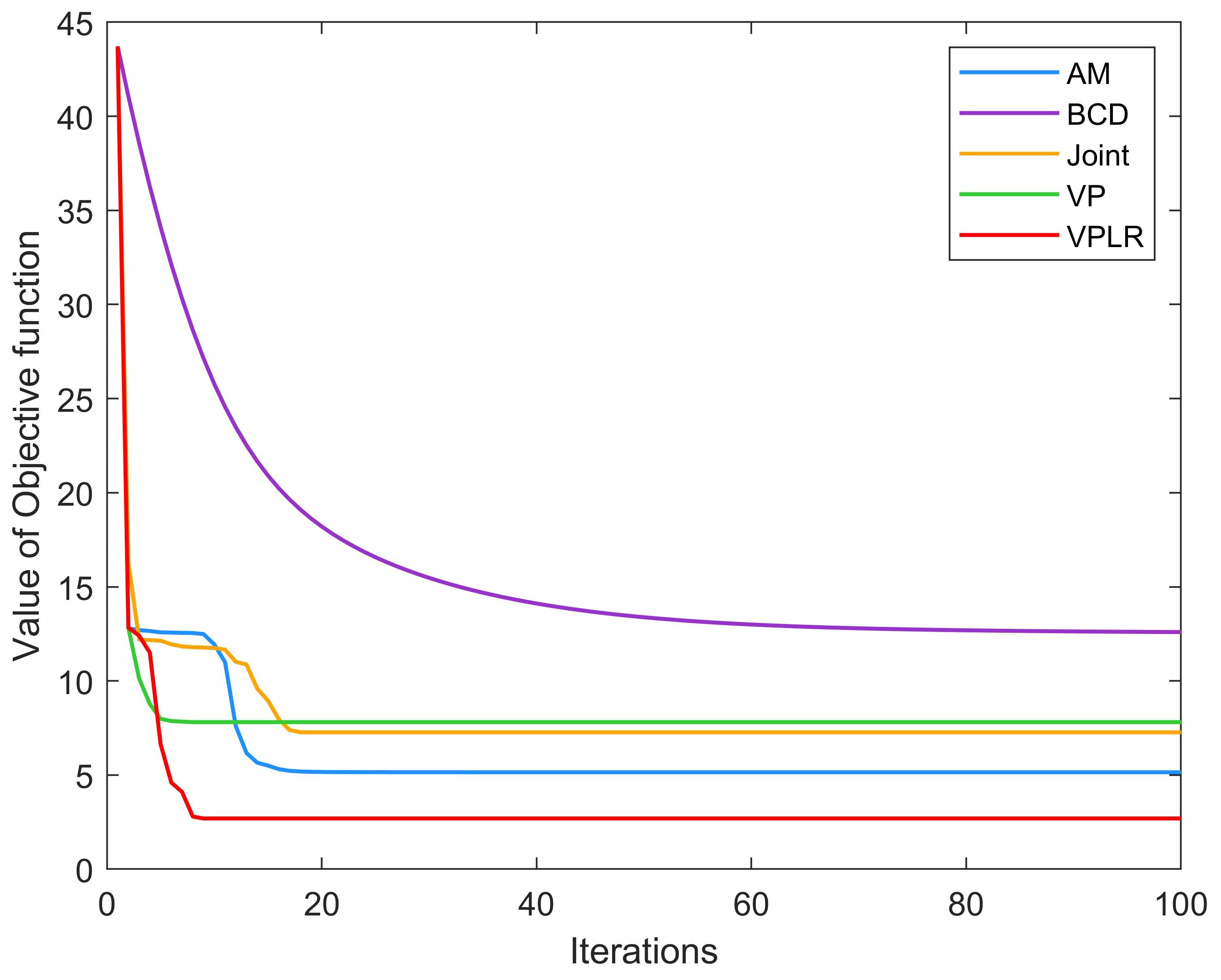
Figure 2: Comparative convergence of different algorithms during iterative process

We use different algorithms to estimate the model parameters, and the results are shown in Fig. 2 and 3. Notably, to verify the impact of large residual, we selected an initial value with a large deviation, resulting in a large residual of the objective function, which is reflected in Fig.2. From Fig. 2, we can clearly see that, since the standard VP algorithm and the proposed VPLR algorithm properly handle the coupling relationship between the linear and nonlinear parameters in the model, the algorithms can converge faster, roughly within 10 iterations, while the joint algorithm and alternating algorithms (AM and BCD) converge relatively slower. Meanwhile, since the VPLR algorithm compensates for the effect of large residual on the Hessian matrix of the reduced objective function during the iteration process, it can find a better solution faster. This can also be observed from Figure 3, which depicts the fitting results of the model estimated by different algorithms: the models estimated by the Joint algorithm, BCD algorithm, and AM algorithm exhibit noticeable deviations in fitting the data; the standard VP algorithm, due to the large initial deviation, is also not conducive to finding a good model to fit the observed data; in contrast, the model found by the VPLR algorithm fits the observed data exceptionally well.

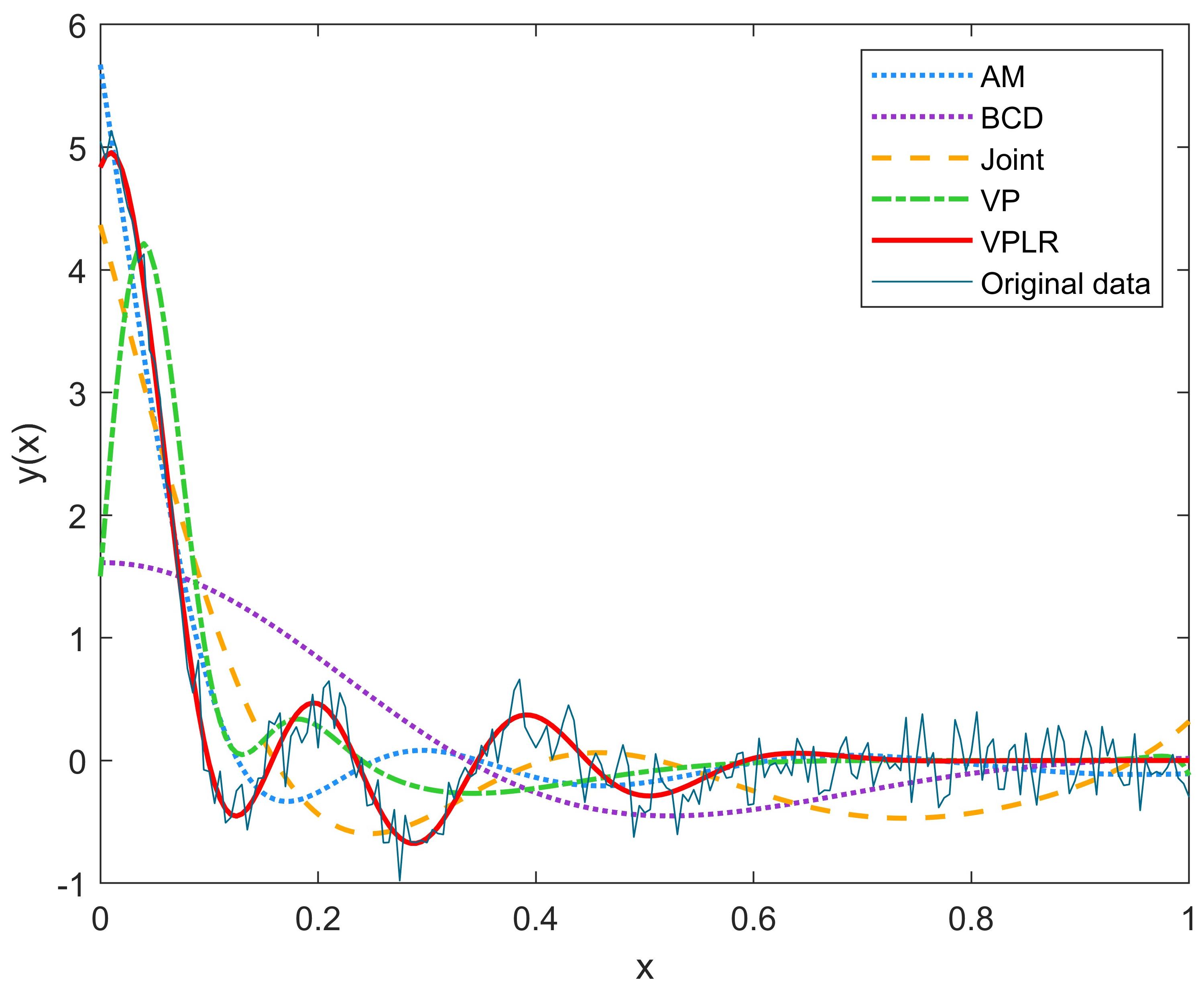
Figure 3: Comparison of the results of fitting observed data to models estimated by different algorithms.

The comparison of the above experimental results demonstrates that the VPLR algorithm proposed in this paper, due to its ability to adeptly handle the coupling relationship between the parameters in the model and compensate for the effect of large residual on the reduced objective Hessian matrix during the iteration process, is capable of finding a superior solution more rapidly.

4.2 Forecasting of Nonlinear Time Series Using the RBF-AR Model

In this subsection, we will use the radial basis function network based autoregressive (RBF-AR) model to model a nonlinear time series - the ozone column thickness data. The RBF-AR($p,m,d$) model is a powerful statistical tool for system modeling [57, 58, 59], which can be expressed as:

$$\left.\left\{\begin{aligned} &y_{t}=\phi_{0}(\boldsymbol{x}_{t-1})+\sum_{i=1}^{p}\phi_{i}(\boldsymbol{x}_{t-1})y_{t-i}+e_{t}\\ &\phi_{i}(\boldsymbol{x}_{t-1})=c_{i,0}+\sum_{j=1}^{m}c_{i,j}\exp\{-\lambda_{j}\|\boldsymbol{x}_{t-1}-\boldsymbol{z}_{j}\|^{2}\}\\ &\boldsymbol{z}_{k}=(z_{k,1},z_{k,2},\cdots,z_{k,d})\\ &\boldsymbol{x}_{t-1}=(y_{t-1},y_{t-2},\cdots,y_{t-d})\end{aligned}\right.\right.$$

where $p,m,d\in\mathrm{Z}^{+}$ denote the orders of the model; $\lambda_{k}$ and $\mathbf{z}_{k}$ $(k=1,\cdots,m)$ represent the radius and centers of the RBF network, respectively. $\boldsymbol{x}_{t}$ encompasses certain explanatory variables within the system; $\phi(\cdot)$ is a nonlinear function.

Next, we employ the RBF-AR($8,1,3$) to fit the ozone column thickness data measured in the Arosa region of Switzerland. This dataset comprises 518 observations of the average thickness of the ozone columns. Following the procedure described in reference [60], we have processed the raw data with a functional transformation to enhance the symmetry of the series and stabilize its variance.

$$\tilde{y}_{i}=\ln(y_{i}-260).$$

The transformed data is shown in Fig. 4.

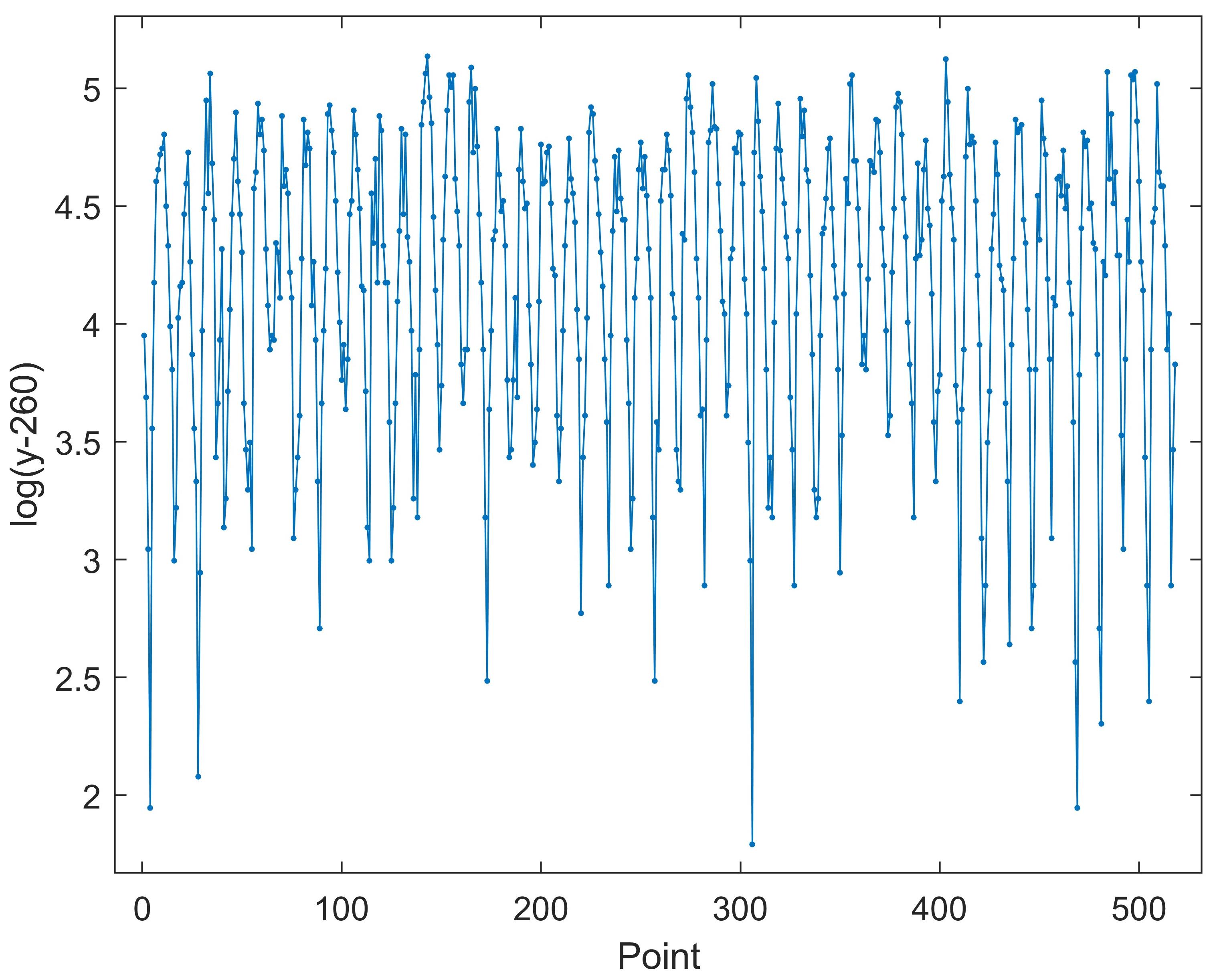
Figure 4: Transformed ozone column data.

In this experiment, the initial 450 data points are employed for model training, while the remaining data points are used to evaluate the predictive capability of the estimated model. We adopt the mean squared error (MSE) as the evaluation metric, which can be expressed as:

$$\text{MSE}=\frac{1}{n}\sum_{i=1}^{n}(y_{i}-\hat{y}_{i})^{2},$$

where $\hat{y}_{i}$ is the output prediction.

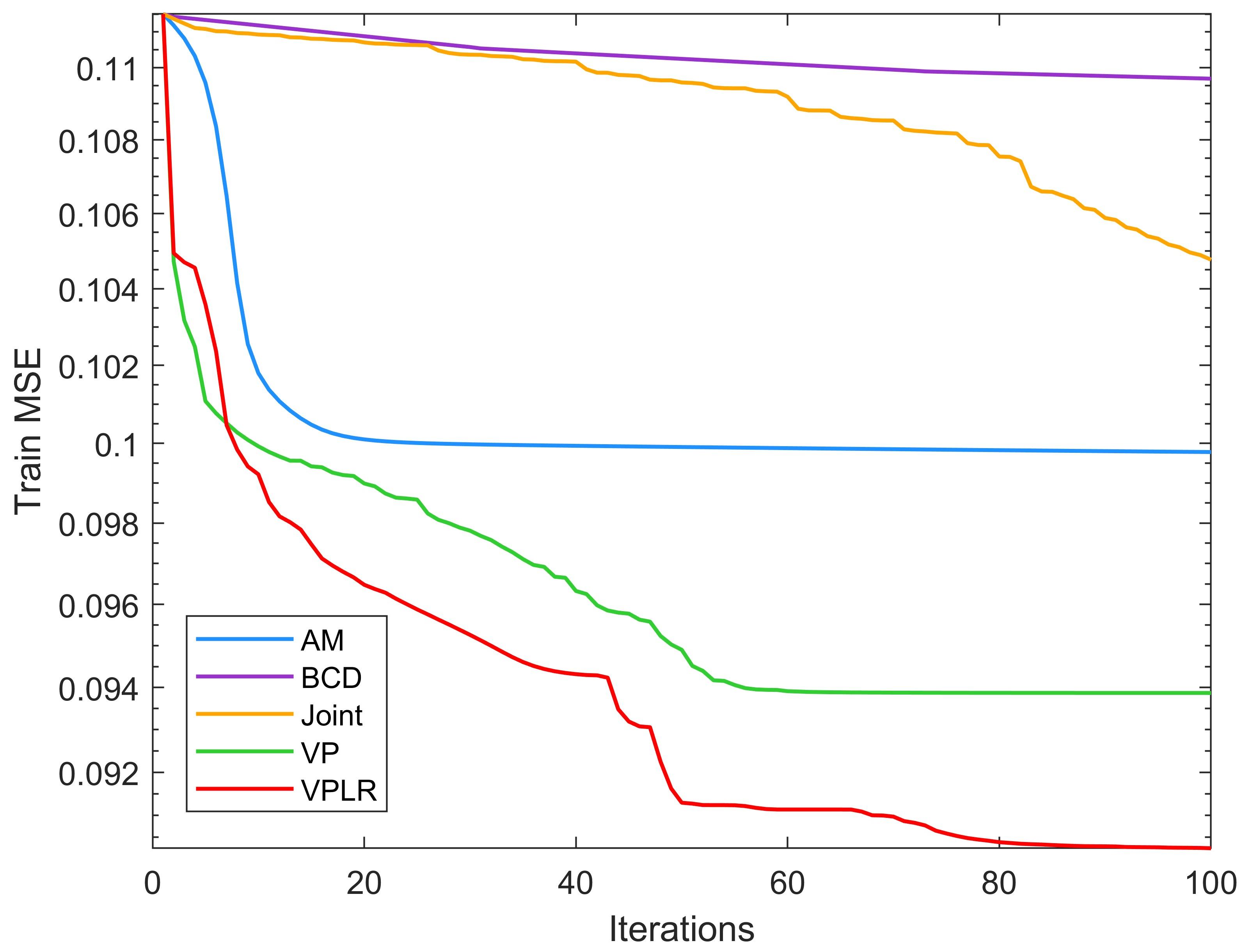
Figure 5: Convergence process of different algorithms using the RBF-AR model to fit ozone column thickness data.

Table 1: Comparison of training and testing errors of different algorithms for fitting ozone data sets using RBF-AR models.

	ALS	BCD	Joint	VP	VPLR
Train MSE	0.0998	0.1097	0.1048	0.0939	$\mathbf{0.0902}$
Test MSE	0.1742	0.2132	0.2003	0.1702	$\mathbf{0.1637}$

As can be seen from Fig. 5, the Joint algorithm, the AM algorithm, and the BCD algorithm converge slowly (especially the Joint algorithm and the BCD algorithm), as they ignore the separable structure of the RBF-AR model and the coupling relationship between the linear and nonlinear parameters in the optimization process. In contrast, the VPLR algorithm and the standard VP algorithm proposed by us can properly handle the coupling relationship between the parameters, which enables them to converge faster. Moreover, since the VPLR algorithm compensates for the effect of the residual on the calculation of the Jacobian matrix of the reduced objective function during the iteration process, it can also find a better solution faster, and the estimated model has a better prediction ability. These are also clearly shown in Table 1, where using the separable structure of the model and handling the coupling relationship between the parameters can help the algorithms find solutions with better prediction ability; and compensating for the effect of large residual can further help the algorithms find better solutions.

The above experimental comparison results also further confirm the effectiveness of the VPLR algorithm proposed in this paper, which can effectively handle the coupling relationship between the parameters and make the algorithm find a model with better explanatory ability faster by compensating for the effect of the residual.

4.3 Fitting Concrete Data Using the RBF Network

In the following part, we utilize the radial basis function (RBF) network

$$y=\sum_{k=1}^{m}c_{k}\exp(-r_{k}\left\|\boldsymbol{Y}-\boldsymbol{Z}\right\|^{2})$$

to model the concrete compressive strength data [61], which consists of 1,030 observations, each containing eight features of concrete mix proportions and the corresponding response of concrete strength.

Figure 6 shows the comparison of the convergence process of different algorithms for identifying RBF networks. From the figure, we can see that, compared with other algorithms, the VPLR algorithm proposed in this paper can achieve a faster convergence rate and find a better RBF network that minimizes the fitting error. The comparison of the fitting errors obtained by different algorithms and the prediction errors of the networks estimated by them are listed in Table 2. From Table 2, we can see more clearly the comparison of different algorithms on the training set and testing set. Compared with other algorithms, the VPLR algorithm obtains the smallest training error, and the network estimated by it has the best prediction performance on the prediction set, that is, it has better generalization ability.

These comparisons show that the algorithm proposed in this paper has obvious advantages for solving large-residual separable nonlinear optimization problems, under the condition of properly handling parameter coupling and compensating for the impact of residual. In addition, from the three experiments in this chapter, we can observe that the local convergence speed of the joint optimization algorithm is slower than that of the VP algorithm, which is consistent with the theoretical analysis in this paper.

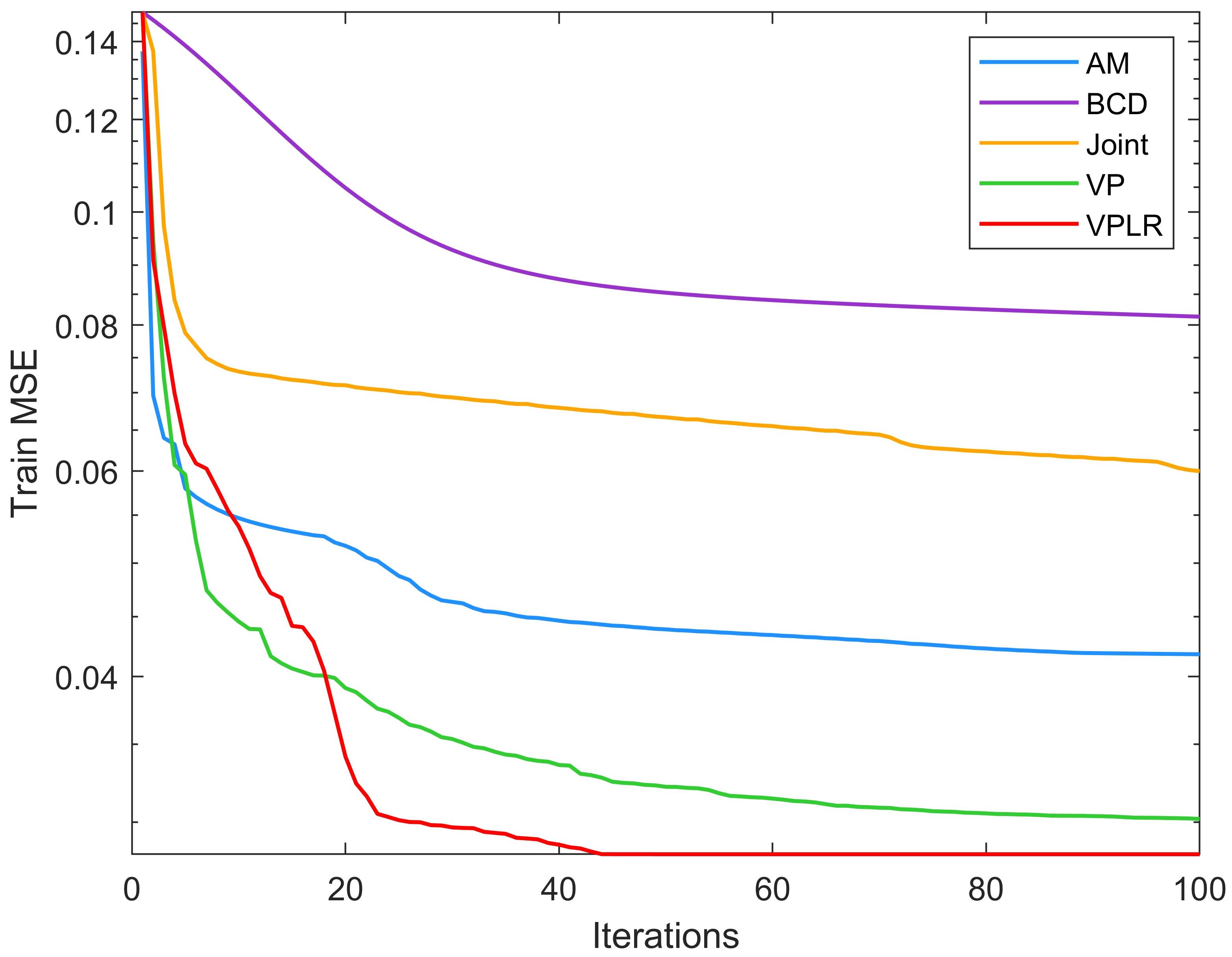
Figure 6: Comparison of the convergence processes of different algorithms for concrete dataset.

Table 2: Comparison of training and testing errors of different algorithms for Concrete data using RBF Networks.

	ALS	BCD	Joint	VP	VPLR
Train MSE	0.0418	0.0813	0.0600	0.0301	$\mathbf{0.0282}$
Test MSE	0.2775	0.1034	0.0655	0.0849	$\mathbf{0.0458}$

5 CONCLUSIONS

Separable nonlinear models are fundamental models in practical applications such as system modeling, data analysis, image processing, and so on. This paper investigates a highly efficient algorithm for identifying these models, namely the VP algorithm, and provides a theoretical analysis framework for the impact of the reduced objective’s approximate Jacobian matrix (i.e., the approximate treatment of the coupling relationship between the linear and nonlinear parameters in the model) on the convergence performance of the VP algorithm. We answer an important theoretical question: under certain conditions, the Kaufman form of the VP algorithm can achieve similar convergence rate as the Golub & Pereyra form. Inspired by the theoretical analysis, we also design a VP algorithm for separable nonlinear optimization problem with large residual, denoted as VPLR, which improves the algorithm’s convergence by compensating the approximate Hessian matrix recursively while handling the coupling relationship between the model parameters. The theoretical research results of this paper fill the gap in this field and provide a strong support for understanding the mechanism of the VP algorithm and expanding its application scenarios.

References

- [1] Nilay Saraf and Alberto Bemporad. An efficient bounded-variable nonlinear least-squares algorithm for embedded mpc. Automatica, 141:110293, 2022.
- [2] Feng Zhou, Min Gan, and CL Philip Chen. Robust model predictive control algorithm with variable feedback gains for output tracking. IEEE Transactions on Industrial Electronics, 68(5):4228–4237, 2020.
- [3] Jing Chen, Manfeng Hu, Yawen Mao, and Quanmin Zhu. Modified multi-direction iterative algorithm for separable nonlinear models with missing data. IEEE Signal Processing Letters, 29:1968–1972, 2022.
- [4] Jing Chen, Yanjun Liu, Min Gan, and Quanmin Zhu. Sequential stabilizing spline algorithm for linear systems: Eigenvalue approximation and polishing. Automatica, 159:111313, 2024.
- [5] Malena I Español and Mirjeta Pasha. Variable projection methods for separable nonlinear inverse problems with general-form tikhonov regularization. Inverse Problems, 2023.
- [6] Zhouchen Lin, Chen Xu, and Hongbin Zha. Robust matrix factorization by majorization minimization. IEEE transactions on Pattern Analysis and Machine Intelligence, 40(1):208–220, 2017.
- [7] Qiwei Sheng, Kun Wang, Thomas P Matthews, Jun Xia, Liren Zhu, Lihong V Wang, and Mark A Anastasio. A constrained variable projection reconstruction method for photoacoustic computed tomography without accurate knowledge of transducer responses. IEEE transactions on Medical Imaging, 34(12):2443–2458, 2015.
- [8] Julianne Chung, Jiahua Jiang, Scot M Miller, and Arvind K Saibaba. Hybrid projection methods for solution decomposition in large-scale bayesian inverse problems. SIAM Journal on Scientific Computing, pages S97–S119, 2023.
- [9] Péter Kovács, Sándor Fridli, and Ferenc Schipp. Generalized rational variable projection with application in ecg compression. IEEE Transactions on Signal Processing, 68:478–492, 2019.
- [10] Maria M Barbieri and Piero Barone. A two-dimensional prony’s method for spectral estimation. IEEE Transactions on Signal Processing, 40(11):2747–2756, 1992.
- [11] Péter Kovács, Gergő Bognár, Christian Huber, and Mario Huemer. Vpnet: variable projection networks. International Journal of Neural Systems, 32(01):2150054, 2022.
- [12] Armin Lederer, Zewen Yang, Junjie Jiao, and Sandra Hirche. Cooperative control of uncertain multi-agent systems via distributed gaussian processes. IEEE Transactions on Automatic Control, 68(5):3091–3098, 2023.
- [13] Elizabeth Newman, Lars Ruthotto, Joseph Hart, and Bart van Bloemen Waanders. Train like a (var) pro: Efficient training of neural networks with variable projection. SIAM Journal on Mathematics of Data Science, 3(4):1041–1066, 2021.
- [14] Gene Golub and Victor Pereyra. Separable nonlinear least squares: the variable projection method and its applications. Inverse Problems, 19(2):R1, 2003.
- [15] Carlo Tomasi and Takeo Kanade. Shape and motion from image streams under orthography: a factorization method. International Journal of Computer Vision, 9:137–154, 1992.
- [16] Je Hyeong Hong and Andrew Fitzgibbon. Secrets of matrix factorization: Approximations, numerics, manifold optimization and random restarts. In Proceedings of the IEEE International Conference on Computer Vision, pages 4130–4138, 2015.
- [17] Fengyuan Hu, Xue Jiang, Junfeng Wang, and Xingzhao Liu. Sar structure-from-motion via matrix factorization. In IGARSS 2023-2023 IEEE International Geoscience and Remote Sensing Symposium, pages 6967–6970. IEEE, 2023.
- [18] N Benjamin Erichson, Peng Zheng, Krithika Manohar, Steven L Brunton, J Nathan Kutz, and Aleksandr Y Aravkin. Sparse principal component analysis via variable projection. SIAM Journal on Applied Mathematics, 80(2):977–1002, 2020.
- [19] Olga Dorabiala, Aleksandr Aravkin, and J Nathan Kutz. Ensemble principal component analysis. arXiv preprint arXiv:2311.01826, 2023.
- [20] Guang-Yong Chen, Hui-Lang Xu, Min Gan, and CL Philip Chen. A variable projection-based algorithm for fault detection and diagnosis. IEEE Transactions on Instrumentation and Measurement, 2023.
- [21] Jing Chen, Junxia Ma, Min Gan, and Quanmin Zhu. Multidirection gradient iterative algorithm: A unified framework for gradient iterative and least squares algorithms. IEEE Transactions on Automatic Control, 67(12):6770–6777, 2022.
- [22] Stéphane Victor, Abir Mayoufi, Rachid Malti, Manel Chetoui, and Mohamed Aoun. System identification of miso fractional systems: parameter and differentiation order estimation. Automatica, 141:110268, 2022.
- [23] Jing Chen, Biao Huang, Min Gan, and CL Philip Chen. A novel reduced-order algorithm for rational models based on arnoldi process and krylov subspace. Automatica, 129:109663, 2021.
- [24] Vivek Khatana and Murti V Salapaka. Dc-distadmm: Admm algorithm for constrained optimization over directed graphs. IEEE Transactions on Automatic Control, 68(9):5365–5380, 2023.
- [25] Moritz Hardt. Understanding alternating minimization for matrix completion. In 2014 IEEE 55th Annual Symposium on Foundations of Computer Science, pages 651–660. IEEE, 2014.
- [26] Yu Yang, Qing-Shan Jia, Zhanbo Xu, Xiaohong Guan, and Costas J Spanos. Proximal admm for nonconvex and nonsmooth optimization. Automatica, 146:110551, 2022.
- [27] He Kong, Mao Shan, Salah Sukkarieh, Tianshi Chen, and Wei Xing Zheng. Kalman filtering under unknown inputs and norm constraints. Automatica, 133:109871, 2021.
- [28] A.M. Buchanan and A.W. Fitzgibbon. Damped newton algorithms for matrix factorization with missing data. In 2005 IEEE Computer Society Conference on Computer Vision and Pattern Recognition (CVPR’05), volume 2, pages 316–322 vol. 2, 2005.
- [29] T Wiberg. Computation of principal components when data are missing. In Proc. of Second Symp. Computational Statistics, pages 229–236, 1976.
- [30] Takayuki Okatani and Koichiro Deguchi. On the wiberg algorithm for matrix factorization in the presence of missing components. International Journal of Computer Vision, 72(3):329–337, 2007.
- [31] Alfonso Landeros, Jason Xu, and Kenneth Lange. Mm optimization: Proximal distance algorithms, path following, and trust regions. Proceedings of the National Academy of Sciences, 120(27):e2303168120, 2023.
- [32] Tristan Van Leeuwen and Aleksandr Y Aravkin. Variable projection for nonsmooth problems. SIAM journal on scientific computing, 43(5):S249–S268, 2021.
- [33] Gene H Golub and Victor Pereyra. The differentiation of pseudo-inverses and nonlinear least squares problems whose variables separate. SIAM Journal on Numerical Analysis, 10(2):413–432, 1973.
- [34] Guang-Yong Chen, Min Gan, Jing Chen, and Long Chen. Embedded point iteration based recursive algorithm for online identification of nonlinear regression models. IEEE Transactions on Automatic Control, 68:4257–4264, 2022.
- [35] Xiaoyong Zeng, Hui Peng, and Feng Zhou. A regularized snpom for stable parameter estimation of rbf-ar (x) model. IEEE Transactions on Neural Networks and Learning Systems, 29(4):779–791, 2017.
- [36] Khaled Laadjal, Mohamed Sahraoui, Antonio J Marques Cardoso, and Acácio Manuel Raposo Amaral. Online estimation of aluminum electrolytic-capacitor parameters using a modified prony’s method. IEEE Transactions on Industry Applications, 54(5):4764–4774, 2018.
- [37] Carl Böck, Péter Kovács, Pablo Laguna, Jens Meier, and Mario Huemer. Ecg beat representation and delineation by means of variable projection. IEEE Transactions on Biomedical engineering, 68(10):2997–3008, 2021.
- [38] Cheol-Taek Kim and Ju-Jang Lee. Training two-layered feedforward networks with variable projection method. IEEE Transactions on Neural Networks, 19(2):371–375, 2008.
- [39] Xiang-Xiang Su, Min Gan, Guang-Yong Chen, Lin Yang, and Jun-Wei Jin. Nonmonotone variable projection algorithms for matrix decomposition with missing data. Pattern Recognition, page 110150, 2023.
- [40] Linda Kaufman. A variable projection method for solving separable nonlinear least squares problems. BIT Numerical Mathematics, 15:49–57, 1975.
- [41] AEB Ruano, DI Jones, and PJ Fleming. A new formulation of the learning problem of a neural network controller. In [1991] Proceedings of the 30th IEEE Conference on Decision and Control, pages 865–866. IEEE, 1991.
- [42] Xiongfeng Song, Wei Xu, Ken Hayami, and Ning Zheng. Secant variable projection method for solving nonnegative separable least squares problems. Numerical Algorithms, 85:737–761, 2020.
- [43] Paul Shearer and Anna C Gilbert. A generalization of variable elimination for separable inverse problems beyond least squares. Inverse Problems, 29(4):045003, 2013.
- [44] Guang-Yong Chen, Shu-Qiang Wang, Min Gan, and C.L.Philip Chen. Insights into algorithms for separable nonlinear least squares problems. IEEE transactions on Image Processing, 30(2):1207–1218, 2021.
- [45] Axel Ruhe and Per Åke Wedin. Algorithms for separable nonlinear least squares problems. SIAM review, 22(3):318–337, 1980.
- [46] Jize Zhang, Andrew M Pace, Samuel A Burden, and Aleksandr Aravkin. Offline state estimation for hybrid systems via nonsmooth variable projection. Automatica, 115:108871, 2020.
- [47] Jonas Sjoberg and Mats Viberg. Separable non-linear least-squares minimization-possible improvements for neural net fitting. In Neural Networks for Signal Processing VII. Proceedings of the 1997 IEEE Signal Processing Society Workshop, pages 345–354. IEEE, 1997.
- [48] Guang-Yong Chen, Shu-Qiang Wang, Min Gan, and CL Philip Chen. Insights into algorithms for separable nonlinear least squares problems. IEEE Transactions on Image Processing, 2020.
- [49] Carl T Kelley. Iterative methods for linear and nonlinear equations. SIAM, 1995.
- [50] Min Gan, C. L. Philip Chen, Guang Yong Chen, and Long Chen. On some separated algorithms for separable nonlinear least squares problems. IEEE Transactions on Cybernetics, 48(10):2866–2874, 2018.
- [51] Jing Chen, Yawen Mao, Min Gan, Dongqing Wang, and Quanmin Zhu. Greedy search method for separable nonlinear models using stage aitken gradient descent and least squares algorithms. IEEE Transactions on Automatic Control, 68(8):5044–5051, 2023.
- [52] Aleksandr Y Aravkin, Dmitriy Drusvyatskiy, and Tristan van Leeuwen. Efficient quadratic penalization through the partial minimization technique. IEEE Transactions on Automatic Control, 63(7):2131–2138, 2017.
- [53] John E Dennis Jr and Robert B Schnabel. Numerical methods for unconstrained optimization and nonlinear equations. SIAM, 1996.
- [54] Sergey Guminov, Pavel Dvurechensky, Nazarii Tupitsa, and Alexander Gasnikov. On a combination of alternating minimization and nesterov’s momentum. In International Conference on Machine Learning, pages 3886–3898. PMLR, 2021.
- [55] Julie Nutini, Issam Laradji, and Mark Schmidt. Let’s make block coordinate descent converge faster: faster greedy rules, message-passing, active-set complexity, and superlinear convergence. Journal of Machine Learning Research, 23(131):1–74, 2022.
- [56] Stephen J Wright. Coordinate descent algorithms. Mathematical Programming, 151(1):3–34, 2015.
- [57] Min Gan, CL Philip Chen, Long Chen, and Chun-Yang Zhang. Exploiting the interpretability and forecasting ability of the rbf-ar model for nonlinear time series. International Journal of Systems Science, 47(8):1868–1876, 2016.
- [58] Hui Peng, Jun Wu, Garba Inoussa, Qiulian Deng, and Kazushi Nakano. Nonlinear system modeling and predictive control using the rbf nets-based quasi-linear arx model. Control Engineering Practice, 17(1):59–66, 2009.
- [59] Hui Peng, Tohru Ozaki, Yukihiro Toyoda, Hideo Shioya, Kazushi Nakano, Valerie Haggan-Ozaki, and Masafumi Mori. Rbf-arx model-based nonlinear system modeling and predictive control with application to a nox decomposition process. Control Engineering Practice, 12(2):191–203, 2004.
- [60] Guang-Yong Chen, Min Gan, and Guo-long Chen. Generalized exponential autoregressive models for nonlinear time series: Stationarity, estimation and applications. Information Sciences, 438:46–57, 2018.
- [61] I-C Yeh. Modeling of strength of high-performance concrete using artificial neural networks. Cement and Concrete Research, 28(12):1797–1808, 1998.