Friedmann’s Universe Controlled by Gauss-Bonnet Modified Gravity

Abstract

The accepted idea that the expansion of the universe is accelerating needs, for compatibility to general relativity, the introduction of some unusual forms of matter. However, several authors have proposed that instead of making weird hypothesis on some yet unobservable species of matter, one should follow the original idea of the first Einstein’s paper on cosmology and consider that in the cosmic scene one has to modify the equations that controls the gravitational metric. This possibility led us to re-examine the evolution of the topological invariant containing two duals in a dynamical universe, the so called Gauss-Bonnet topological invariant. The particular interest on this invariant is due to the fact that in a homogeneous and isotropic universe this invariant drives the cosmic acceleration. In a decelerating scenario and as a necessary previous condition of an ulterior acceleration this invariant must have an extremum identified to its maximum value. We will examine the conditions for this to occur, and a description of the universe with epochs of accelerated and decelerated expansion.

I Introduction

Modified theories of gravity have been proposed in order to account for astronomical data, like the cosmic late acceleration. Two of such propositions that have been gaining notoriety are the f(R) theory and the Gauss-Bonnet (GB) topological invariant modified gravity [1, 2, 3, 4]. In GB modified gravity it makes use of the topological invariant of the same name, which is only an invariant in 4D space-time, commonly expressed as $\mathcal{G}$.

This topological invariant $\mathcal{G}$ by itself does not affect the dynamics of General Relativity in 4D when added to the Einstein-Hilbert action, instead, there are three basic ways to implementing it. First, by coupling $\mathcal{G}$ to a scalar field $\phi$ [5]. Second, by considering a nontrivial function of the topological invariant, $f(\mathcal{G})$ modified gravity. And third, by implementing the topological invariant to a Einstein-Hilbert action of higher dimension $D$, in which $\mathcal{G}$ is no longer a topological invariant, and taking the limit $D\rightarrow 4$, yielding nontrivial modified dynamics [6]. Some groups had used observational data in order to find constraints to different approaches to GB modified gravity [7, 8, 9, 10]. Great reviews of modified theories of gravity can be found at [11, 12, 13, 14].

In this present work we use the $f(\mathcal{G})$ Gauss-Bonnet Modified Gravity approach, by applying the simplest non-trivial function of $\mathcal{G}$, we peer into its consequences on a homogeneous and isotropic Friedmann’s geometry. Section III. gives a very brief definition of topological invariants in 4D. Section IV. presents the standard $f(\mathcal{G})$ gravity; subsection IV.a. presents a relationship between $f(\mathcal{G})$ and the Fierz representation of a spin-2 particle. Section V. applies the theory to the Friedmann’s universe; subsection V.A. deals with the case for $\mathcal{G}=constant$, which yields an important constraint to filter out non-physical solutions; subsection V.B. considers the simplest non-trivial function of $\mathcal{G}$, that is $f(\mathcal{G})=\sigma\mathcal{G}^{2}$; first we assume an empty space-time, which produces a 2D dynamical system, and a complete qualitative description of numerical solutions near and around the critical points is presented; and second, we assume cosmic dust as source, producing a 3D dynamical system, and present a set of qualitative behavior of numerical solutions. Section VI. the conclusion.

II Topological Invariants in 4D

There are two topological invariants in a 4-d Riemannian geometry, that is

$$I=\int\sqrt{-g}\,A\,d^{4}x$$

$$II=\int\sqrt{-g}\,\mathcal{G}\,d^{4}x$$

where

$$A=R_{\alpha\beta\mu\nu}^{*}\,R^{\alpha\beta\mu\nu}$$

and $\mathcal{G}$ is the Gauss-bonnet topological invariant

$$\mathcal{G}=R_{\alpha\beta}^{*}{}_{\mu\nu}^{*}\,R^{\alpha\beta\mu\nu}.$$

The dual is defined for any anti-symmetric tensor $F_{\mu\nu}$ as

$$F_{\mu\nu}^{*}=\frac{1}{2}\,\eta_{\mu\nu\alpha\beta}\,F^{\alpha\beta}$$

$$\eta_{\mu\nu\alpha\beta}=\sqrt{-g}\,\epsilon_{\mu\nu\alpha\beta}$$

where $\epsilon_{\mu\nu\alpha\beta}$ is the completely anti-symmetric Levi-Cività symbol.

We note that the invariant $\mathcal{G}$ can be written in terms of the curvature tensor (without the dual operation) by the identity

$$\mathcal{G}=-R_{\alpha\beta\mu\nu}\,R^{\alpha\beta\mu\nu}+4\,R_{\mu\nu}\,R^{\mu\nu}-R^{2}.$$

This $\mathcal{G}$ satisfies the identity

$$\tensor{R}{{}^{\overset{\ast}{\mu\nu}}{}^{\overset{\ast}{\alpha\beta}}}\tensor{R}{{}^{\epsilon}_{\nu}{}_{\alpha}{}_{\beta}}=\frac{1}{4}\mathcal{G}\tensor{g}{{}^{\mu}{}^{\epsilon}}.$$

III Modified Gravity via Gauss-Bonnet Topological Invariant

For an arbitrary function $f(\mathcal{G})$, the variation of the action

$$S=\int\sqrt{-g}\left(R+f(\mathcal{G})+L_{m}\right),$$ (1)

where $L_{m}$ is the matter Lagrangian, leads to the following set of dynamic equations,

$$R_{\mu\nu}-\frac{1}{2}Rg_{\mu\nu}+Z_{\mu\nu}=-T_{\mu\nu},$$ (2)

where $Z_{\mu\nu}$ is defined as

$$Z_{\mu\nu}\equiv\frac{1}{2}\left(f^{\prime}\mathcal{G}-f\right)g_{\mu\nu}+2\tensor{H}{{}^{\alpha}_{\;(\mu\nu);\alpha}},$$ (3)

$$\tensor{H}{{}^{\mu}{}^{\nu}{}^{\beta}}\equiv f^{\prime\prime}\mathcal{G}_{,\sigma}\tensor{R}{{}^{\overset{\ast}{\mu\nu}}{}^{\overset{\ast}{\beta\sigma}}},$$ (4)

where $f^{\prime}=\frac{df}{d\mathcal{G}}$.

Note that contraction of the last two indices of $\tensor{H}{{}^{\mu}{}^{\nu}{}^{\alpha}}$ implies the identity

$$\tensor{H}{{}^{\mu}{}^{\nu}_{\nu}}=-f^{\prime\prime}\mathcal{G}_{,\nu}\left(\tensor{R}{{}^{\mu}{}^{\nu}}-\frac{1}{2}R\tensor{g}{{}^{\mu}{}^{\nu}}\right).$$

III.1 The Curious Presence of a Fierz Tensor $H_{\alpha\beta\mu}$ Representing a Spin-2

Let us show that such quantity $\tensor{H}{{}^{\mu}{}^{\nu}{}^{\beta}}$ defined by equation (4) may be associated to a spin-2 field. We start by remembering that there are two basic representations to deal with a spin-2 field that we call the Einstein and the Fierz representations (both were introduced by Fierz):

• Einstein representation: $\varphi_{\mu\nu},$

• Fierz representation: $F_{\alpha\beta\mu}.$

The tensor $\varphi_{\mu\nu}$ is symmetric and deals with 10 components. The tensor $F_{\alpha\beta\mu}$ has the symmetries

$$\tensor{F}{{}^{\mu}{}^{\nu}{}^{\beta}}=-\tensor{F}{{}^{\nu}{}^{\mu}{}^{\beta}},$$

which states that this tensor has 24 independent components. The second property states that the dual has no trace, that is

$$\tensor{F}{{}_{\mu}{}_{\nu}{}_{\beta}}+\tensor{F}{{}_{\beta}{}_{\mu}{}_{\nu}}+\tensor{F}{{}_{\nu}{}_{\beta}{}_{\mu}}=0$$

or, equivalently

$$\tensor{F}{{}^{\overset{\ast}{\mu\alpha}}_{\alpha}}=0,$$

which reduces this number to 20. The identity

$$\tensor{F}{{}^{\mu}{}^{\nu}{}^{\beta}_{;\beta}}=0$$

makes this number to 14, and finally, the property of vanishing trace

$$\tensor{F}{{}^{\alpha}{}^{\mu}_{\mu}}=0$$

reduces the number of independent components to 10.

It is a simple direct exercise to show that the tensor $\tensor{H}{{}^{\mu}{}^{\nu}{}^{\alpha}}$ defined as for equation (4),

$$f^{\prime\prime}\mathcal{G}_{,\sigma}\tensor{R}{{}^{\overset{\ast}{\mu\nu}}{}^{\overset{\ast}{\beta\sigma}}},$$

satisfies all these conditions showing that there is a spin-2 tensor hidden in the above dynamics constructed with the invariant $\mathcal{G}$.

The tensor $\tensor{H}{{}^{\mu}{}^{\nu}{}^{\beta}}$ has four properties:

• Anti-symmetric in the first two indices: $\tensor{H}{{}^{\mu}{}^{\nu}{}^{\beta}}=-\tensor{H}{{}^{\nu}{}^{\mu}{}^{\beta}}$

• Cyclic identity: $\tensor{H}{{}_{\mu}{}_{\nu}{}_{\beta}}+\tensor{H}{{}_{\beta}{}_{\mu}{}_{\nu}}+\tensor{H}{{}_{\nu}{}_{\beta}{}_{\mu}}=0\Leftrightarrow\tensor{H}{{}^{\overset{\ast}{\mu\alpha}}_{\alpha}}=0$

• Null divergent in the last indice: $\tensor{H}{{}^{\mu}{}^{\nu}{}^{\beta}_{;\beta}}=0$

• Contraction of the last two indices implies $:\tensor{H}{{}^{\mu}{}^{\nu}_{\nu}}=-X_{\nu}\left(\tensor{R}{{}^{\mu}{}^{\nu}}-\frac{1}{2}R\tensor{g}{{}^{\mu}{}^{\nu}}\right)$

So the quantity $\tensor{H}{{}^{\mu}{}^{\nu}{}^{\beta}}$ satisfies all properties of the Fierz tensor, which is a representation of a spin-2 field via a 3-rank tensor, see [15].

IV Gauss-Bonnet Modified Gravity in Friedmann’s Universe

Let’s consider the homogeneous and isotropic Friedmann’s metric,

$$ds^{2}=dt^{2}-a(t)^{2}(dx^{2}+dy^{2}+dz^{2}),$$ (5)

where $a(t)$ is the scale factor. Using the definition of the Hubble parameter $H\equiv\dot{a}/a$, the Gauss-Bonnet topological invariant yields

$$\mathcal{G}=-24\frac{\ddot{a}\dot{a}^{2}}{a^{3}}=-24(\dot{H}+H^{2})H^{2},$$ (6)

note that the sign of $\mathcal{G}$ indicates the sign of the acceleration of the scale factor.

From (2), the new term $Z_{\mu\nu}$ can be treated as geometric source and in the case of metric (5) when $\mathcal{G}$ is only a function of time it can be associated to a perfect fluid [16], that is,

$$R_{\mu\nu}-\frac{1}{2}Rg_{\mu\nu}=-Z_{\mu\nu}-T_{\mu\nu},$$ (7)

where $Z_{\mu\nu}$ can be written under the form

$$Z_{\mu\nu}=(\rho_{Z}+p_{Z})v_{\mu}v_{\nu}-p_{Z}g_{\mu\nu},$$ (8)

Thus the corresponding geometric density $\rho_{Z}$ and geometric pressure $p_{Z}$ are given by,

$$\rho_{z}=\frac{1}{2}\left(f^{\prime}\mathcal{G}-f\right)+12f"\dot{\mathcal{G}}$$ (9)

and

$$p_{z}=-\frac{1}{2}\left(f^{\prime}\mathcal{G}-f\right)-4\left[\left(f^{\prime\prime\prime}\dot{\mathcal{G}}^{2}+f"\ddot{\mathcal{G}}\right)\left(\frac{\dot{a}}{a}\right)^{2}+2f"\dot{\mathcal{G}}\frac{\ddot{a}\dot{a}}{a^{2}}\right].$$ (10)

The modified dynamical equations from (7) are straightforward,

$$3H^{2} =\rho_{Z}+\rho_{m},$$ (11)

$$2\dot{H}+3H^{2} =-p_{Z}-p_{m},$$ (12)

where the energy-matter source satisfies the conservation law,

$$0=\dot{\rho_{m}}+3(\rho_{m}+p_{m})H.$$ (13)

We’ll see later that this system can have solutions where the Gauss-Bonnet topological invariant $\mathcal{G}$ is cyclically dampened, changing it’s sign periodically, which could be used to describe a universe with stages of acceleration and deceleration, but first let us consider the case where $\mathcal{G}$ is constant for an interval or indefinitely.

IV.1 The Case with $\mathcal{G}=cte$

The most simple behavior we could get from $\mathcal{G}$ is a constant , let

$$\mathcal{G}\equiv\alpha,$$ (14)

so $\dot{\mathcal{G}}=0$, then the geometric density and pressure are constants and such that it is equivalent to a cosmological constant, that is, $\rho_{Z}+p_{Z}=0.$

It then follows

$$0=\dot{\mathcal{G}}=-24(\ddot{H}H^{2}+4H^{3}\dot{H}+2H\dot{H}^{2}),$$ (15)

Let us define $x\equiv\dot{H}$ and $y\equiv H.$ We can then write eq. (15), as a non-linear autonomous planar dynamical system,

$$\dot{x}= -4xy-2\frac{x^{2}}{y},$$ (16)

$$\dot{y}= x.$$ (17)

It then follows

$$y\frac{dx}{dy}+2x=-4y^{2},$$ (18)

which is a Briout-Bouquet’s differential equation. A type of solution is given by

$$x(y)=-y^{2},$$ (19)

substituting $x=\dot{H}$ and $y=H$, and solving the corresponding differential equation gives the solution for $H$,

$$H=\frac{1}{t+K_{1}},$$ (20)

and for the scale factor $a(t)$

$$a(t)=K_{2}(t+K_{1}),$$ (21)

where $K_{1}$ and $K_{2}$ are constants that depend on the initial conditions.

So if $\mathcal{G}$ is constant then the scale factor increases or decreases linearly over time, and the Hubble parameter presents a singularity at $t=-K_{1}$. Consider the two equations of evolution (11) and (12), which relate the energy $\rho_{m}$ and the pressure $p_{m}$ to the Hubble parameter and the geometric density and pressure, that is,

$$\rho_{m}= \frac{3}{(t+K_{1})^{2}}-\rho_{\alpha}$$ (22)

$$p_{m}= -\frac{1}{(t+K_{1})^{2}}+\rho_{\alpha}.$$ (23)

From (22) we see that if the geometric density $\rho_{\alpha}$ is less or equal to zero, then $\rho_{m}$ is always positive; but if $\rho_{\alpha}$ is positive, then $\rho_{m}$ will be positive only in the interval

$$-\sqrt{\frac{3}{\rho_{\alpha}}}-K_{1}\leq t\leq\sqrt{\frac{3}{\rho_{\alpha}}}-K_{1},$$ (24)

which depends on the value of $\alpha$ and initial conditions. In other words, if the geometric density $\rho_{Z}$ is positive, then, in order for $\rho_{m}$ to be strictly positive, the topological invariant $\mathcal{G}$ cannot be constant indefinitely but must vary over time. This may be useful later in order to filter only solutions with $\rho_{m}\geq 0$.

IV.2 Case with $f(\mathcal{G})=\sigma\mathcal{G}^{2}$

The next simple non-trivial case we can consider is with the function $f(\mathcal{G})=\sigma\mathcal{G}^{2}$. In this case the geometric density and pressure assume the form,

$$\frac{\rho_{z}}{\sigma}= \frac{\mathcal{G}^{2}}{2}+24\dot{\mathcal{G}}H^{3},$$ (25)

$$\frac{p_{z}}{\sigma}= -\frac{\mathcal{G}^{2}}{2}-8\left[\ddot{\mathcal{G}}H^{2}+2\dot{\mathcal{G}}H\left(\dot{H}+H^{2}\right)\right],$$ (26)

and we have to solve the set of differential equations,

$$3H^{2}= \rho_{Z}+\rho_{m},$$ (27)

$$2\dot{H}+3H^{2}= -p_{Z}-p_{m},$$ (28)

$$0= \dot{\rho_{m}}+3(\rho_{m}+p_{m})H,$$ (29)

$$\mathcal{G}= -24(\dot{H}+H^{2})H^{2}.$$ (30)

IV.2.1 Consider an Empty Space-Time

Let us consider the case with an empty space-time. Under these conditions equation (29) is identically zero. Combining equations (25), (26), (27) and (28), yields equation (30). Then, in empty space-time, we only have to deal with equations (27) and (30), which greatly simplifies our problem to an autonomous planar dynamical system. Putting $\dot{\mathcal{G}}$ and $\dot{H}$ in evidence in (27) and (30), we obtain,

$$\dot{\mathcal{G}}= \frac{1}{24H^{3}}\left[\frac{3H^{2}}{\sigma}-\frac{\mathcal{G}^{2}}{2}\right],$$ (31)

$$\dot{H}= -\frac{\mathcal{G}}{24H^{2}}-H^{2}.$$ (32)

This 2D dynamical system represents the whole problem in an empty space-time. Its numerical solutions will prove useful in giving a map to look for certain types of structures and behaviors in the complete problem with energy-matter sources, which is a dynamical system of higher dimension.

For $\dot{\mathcal{G}}=0$ and $\dot{H}=0$, the equilibrium points in the phase space $(\mathcal{G}(t)\times H(t))$ are $\mathcal{G}_{0}=-\frac{-1}{\sigma^{2/3}}\left(\frac{3}{2}\right)^{\frac{1}{3}}$ and $H_{0}=\pm\frac{1}{\left({\sigma 96}\right)^{1/6}}$, so the constant $\sigma$ must be positive in order for the equilibrium points to be real. Observe that the region $H=0$ is a singularity region, and for the origin $H=\mathcal{G}=0$, the system is undefined.

The next step is to determine the behavior of solutions near the equilibrium points. For this we analyze the Jacobian matrix of the system in the equilibrium points, $a=\left(\frac{\partial\dot{\mathcal{G}}}{\partial\mathcal{G}}\right)_{(\mathcal{G}_{0},H_{0})}$, $b=\left(\frac{\partial\dot{\mathcal{G}}}{\partial H}\right)_{(\mathcal{G}_{0},H_{0})}$, $c=\left(\frac{\partial\dot{H}}{\partial\mathcal{G}}\right)_{(\mathcal{G}_{0},H_{0})}$ and $d=\left(\frac{\partial\dot{H}}{\partial H}\right)_{(\mathcal{G}_{0},H_{0})}$, and compute the eigenvalues of this matrix,

$$\begin{vmatrix}a-\lambda&b\\ c&d-\lambda\end{vmatrix}=0.$$ (33)

It turns out that the two eigenvalues are real and of opposite signs for both equilibrium points, so these equilibrium points are saddle points, that is, trajectories near the equilibrium points are attracted or repelled depending on the direction they approach these points (see [17]).

Now to gain more information on the solutions for this problem we can numerically integrate the solutions for given initial conditions. To numerically integrate the solutions I assumed $\sigma\equiv 1$, and using the Runge–Kutta method ([18]), integrating for different initial conditions inside the interval $[\mathcal{G}=-2...1,H=-1...1]$ which contains the two equilibrium saddle points, gives the behavior map in figure 1.

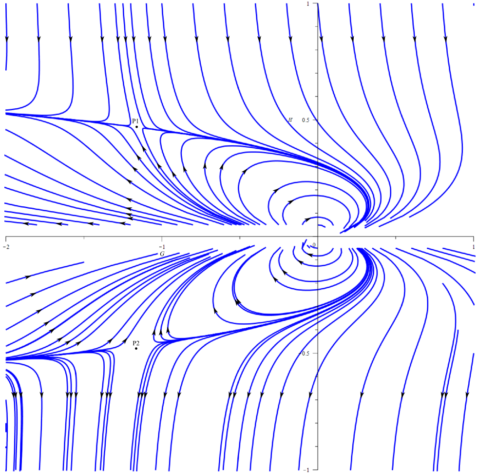
Figure 1: Integral solutions for the 2D dynamical system in the phase space $[\mathcal{G}(t)\times H(t)]$. The points $P1$ and $P2$ are the corresponding equilibrium points of the system. Observe that the $\mathcal{G}$ axis is a singularity for the system and we cannot infer their behavior numerically.

Numerical solutions are only possible if not near the region of singularity of the system, but through approximation it is possible to determine the behavior of solutions near the singularity region (for $H\approx 0$). From (31) and (32) it follows,

$$\frac{\dot{H}}{\dot{\mathcal{G}}}=\frac{dH}{d\mathcal{G}}=-H\frac{\left(\mathcal{G}+24H^{4}\right)}{3H^{2}-\frac{\mathcal{G}^{2}}{2}}.$$ (34)

For $|H|<<1$ and $|\mathcal{G}|>>1$, equation (34) simplifies to $\frac{dH}{d\mathcal{G}}\approx 0$, with solution $H(t)\approx cte$, that is, in the phase space $H(t)$ is constant near the $\mathcal{G}$ axis but away from it’s origin. Let us focus now on what happens to solutions near the origin of the phase space, since $\mathcal{G}\approx 0$ and $H\approx 0$, the $H^{4}$ term can be dropped out compared to $\mathcal{G}$ in the equation (34), yielding

$$\frac{dH}{d\mathcal{G}}\approx-\frac{H\mathcal{G}}{3H^{2}-\frac{\mathcal{G}^{2}}{2}},$$ (35)

which the solutions are given by,

$$H(\mathcal{G})=\frac{1}{12a}\left[1-\sqrt{1-24a^{2}\mathcal{G}^{2}}\right],$$ (36)

and

$$H(\mathcal{G})=\frac{1}{12b}\left[1+\sqrt{1-24b^{2}\mathcal{G}^{2}}\right],$$ (37)

where $a$ and $b$ are constants that depend on the initial conditions. We note the value of $H(t)$ is bounded. The plots of (36) and (37), for different values for $a$ and $b$, are given in figures 2 and 3.

Figure 2: Plots of the solution (36) for different initial conditions.

Figure 3: Plots of the solution (37) for different initial conditions.

The last step, to understand the whole qualitative picture for the behavior of this simplified problem, is to determine how the numerical solutions given in figure 1 interact with the solutions near the origin of the phase space (36) and (37). We can take a direct approach, first consider the solution (36) with an arbitrary value for $a$, because of its square root, both $\mathcal{G}$ and $H$ have two extreme values in this solution; so choosing one of the extreme values and considering them as initial conditions for the 2D dynamical system (31) and (32), we can numerically integrate to obtain an integral solution. Two things can happen to this integral solution, first it can grow away from the origin of the phase space (see figure 1), or it can go back to the origin in two ways: it can go back to the original solution (36), in which case the integral solution is cyclic closed; or it can return but for a different value for the constant $a$ in (36), in which case the integral solution is cyclic open, or have a vortex like behavior. The result is, depending on the initial conditions chosen, the integral solution grows away from the origin or it cycles back in a vortex like behavior nearing the origin of the phase space, figure 4 shows some examples of the first result, and figure 5 shows an example of the second result.

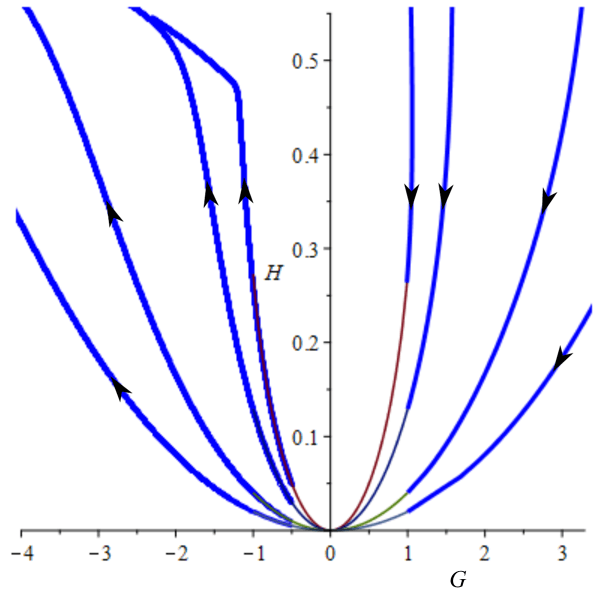
Figure 4: Examples of integral solutions that pass one time through the origin of the phase space $\mathcal{G}\times H$.

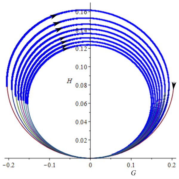
Figure 5: One example of an integral solution presenting an open cyclic behavior (vortex like) near the origin, each time passing through the origin with an smaller arch of travel, that is, the origin acts as an attraction pole.

The figures 1, 4 and 5 give us a summary of the global behavior for the 2D dynamical system (31) and (32). Focusing for $H$ positive, the phase space can be divided into four quadrants, see figure 6. The first quadrant (I) gives us initial conditions where the Hubble parameter $H$ decreases to a minimum positive value and increases afterwards; the second quadrant (II) have initial conditions with integral solutions that converge to the origin of the phase space and are connected to the fourth quadrant (IV), so for initial conditions in (II) the Hubble parameter decreases to zero and increases afterwards in region (IV); and in region (III) the initial conditions result in integral solutions that are open cyclic around the origin of the phase space.

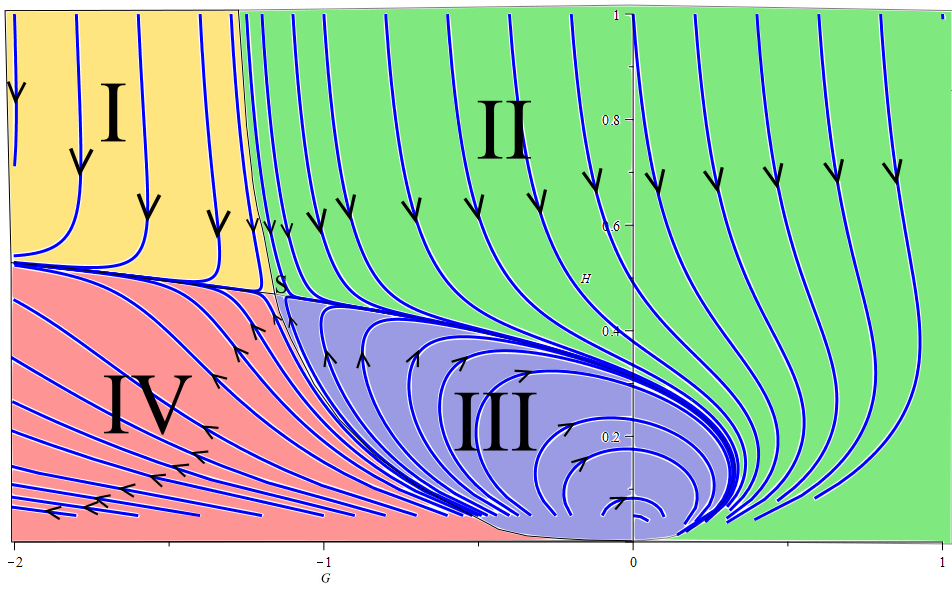
Figure 6: Global behavior of the 2D dynamical system(31) and (32) for $H$ positive. Quadrants (II) and (IV) are connected through the origin, and quadrant (III) have open cyclic solutions attracted to the origin.

So now, having a global qualitative behavior for the empty space-time problem, this gives us a map of behavior to look for in the real case with energy-matter sources. The complete problem is given by the set of equations (27) through (30), for an empty space-time this set yields a 2D dynamical system, and adding matter-energy source yields a higher dimension dynamical system. Figures 1 and 6 provide a rough idea of how the integral solutions behave in these higher dimensional cases.

Depending on the initial conditions, it’s possible to describe an empty Friedmann’s universe in which the topological invariant $\mathcal{G}$ changes sign periodically, from (6) it implies that the acceleration of the scale factor $a(t)$ changes sign periodically, but the Hubble parameter $H$ is always positive or negative, in other words, it can describe an empty universe that is always expanding but periodically accelerating and decelerating, and moreover, the intensity of this acceleration and deceleration decreases over time.

IV.2.2 Friedmann’s Universe with Cosmic Dust

Let us consider now a Friedmann’s universe with cosmic dust. The set of differential equations becomes

$$3H^{2}= \rho_{Z}+\rho_{m},$$ (38)

$$2\dot{H}+3H^{2}= -p_{Z},$$ (39)

$$0= \dot{\rho_{m}}+3\rho_{m}H,$$ (40)

$$\mathcal{G}= -24(\dot{H}+H^{2})H^{2}.$$ (41)

Knowing the expressions for $\rho_{Z}$ and $p_{Z}$, equations (38) and (40) are applied into (39), yielding equation (41), that is, the second dynamic equation is redundant. This simplifies our problem to a 3D autonomous dynamical system in terms of the independent variables $\mathcal{G}(t)$, $H(t)$ and $\rho_{m}(t)$, that is,

$$\dot{\mathcal{G}}= \frac{1}{24\sigma H^{3}}\left[3H^{2}-\sigma\frac{Q^{2}}{2}-\rho_{m}\right],$$ (42)

$$\dot{H}= -\frac{\mathcal{G}}{24H^{2}}-H^{2},$$ (43)

$$\dot{\rho_{m}}= -3\rho_{m}H.$$ (44)

The equilibrium points of the system obtained by setting $\dot{\mathcal{G}}=0$, $\dot{H}=0$ and $\dot{\rho_{m}}=0$ are,

$$\mathcal{G}_{o}= -\left(\frac{3}{2\sigma^{2}}\right)^{\frac{1}{3}},$$ (46)

$$H_{o}= \pm\left(\frac{1}{96\sigma}\right)^{\frac{1}{6}},$$ (47)

$$\rho_{m_{o}}= 0,$$ (48)

which are the same equilibrium points as the case of an empty universe. The eigenvalues of the Jacobian matrix of the system, applied at the equilibrium points, have mixed signs, this implies they behave as saddle points for the integral solutions, just like in the empty space case.

Numerical solutions to this system present behaviors like those observed in the empty space case, that is, for $H(t)$ and $\sigma$ positive, solutions in which the Hubble parameter decreases to a minimum positive or zero value and increases afterwards, or open cyclic behavior in the phase space. Since now we’re dealing with a 3D dynamical system, a compilation of integral solutions in one 3D graph on the phase space becomes convoluted. A sample of two integral solutions, representing the two described behaviors, with given initial conditions, are given below:

In figures 7, 8, 9 and 10 we have a case of integral solution with cyclic behavior. This shows that the cosmic dust has a dampening effect on the evolution of the system, the integral solution does not necessarily need to pass through the origin in the $\mathcal{G}\times H$ phase plane (as seen in figure 7); the Hubble parameter $H$ starts with an initial value and then decreases periodically over time, like a ball bouncing from a surface a few times, approaching a stable value (as observed in figure 8); the topological invariant $\mathcal{G}$ changes its sign a few times until a point in time when it approaches a stable value (as viewed in figure 9), that is, it describes a Friedmann’s universe that goes through epochs of accelerated and decelerated expansion, approaching a stable value with zero acceleration; and finally, the matter density decreases as expected.

Figures 11, 12, 13 and 14 show a case where the Hubble parameter has only one minimum positive value, and the topological invariant changes sign only one time.

One important qualitative result here is that, given a positive value for $\sigma$, and fixed initial conditions for $\mathcal{G}(0)$ and $H(0)=0$, the initial value of the cosmic dust density $\rho_{m}(0)$ will dictate which type of behavior the system will develop, that is, if the Hubble parameter will have only one minimum value, or have a cyclic behavior with epochs of acceleration and deceleration.

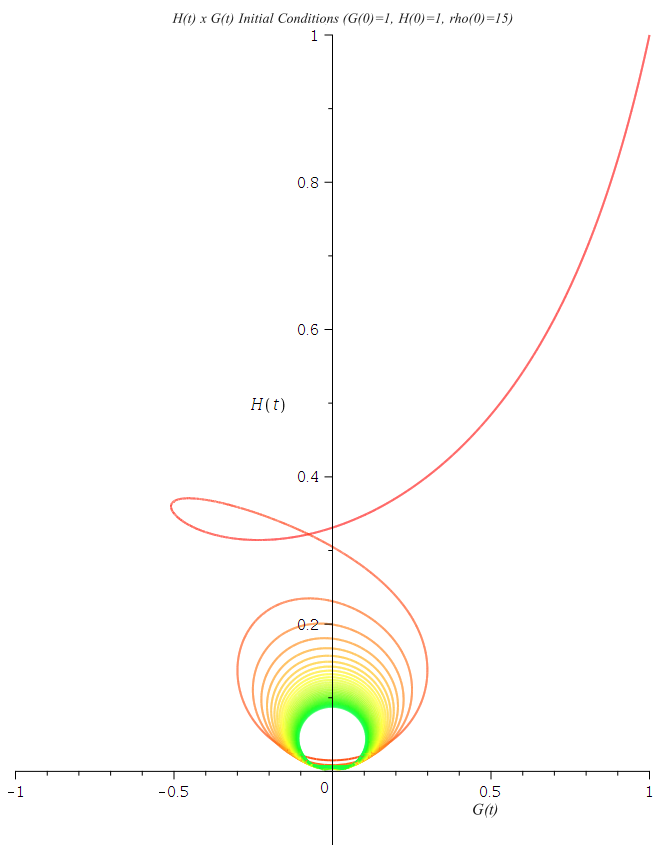
Figure 7: Plot of $\mathcal{G}(t)\times H(t)$ for the Integral solution in the phase space $[\mathcal{G}\times H\times\rho_{m}]$ with initial condition $\mathcal{G}(0)=1$, $H(0)=1$, $\rho(0)=15$. Observe that this is a 3D phase space, so the path of the integral solution doesn’t cross with itself but rather the path is flattened out in the plane $\mathcal{G}\times H$.

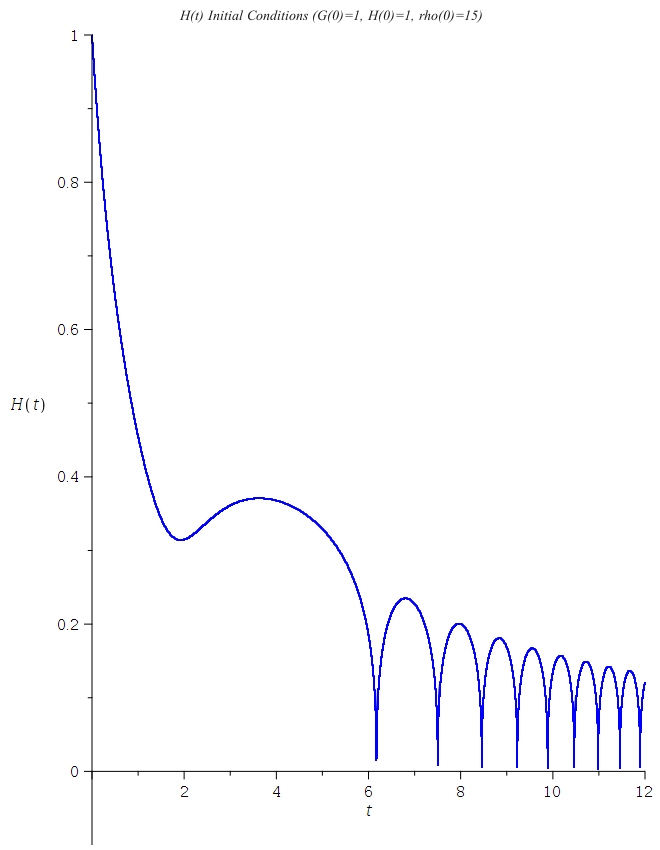
Figure 8: Plot of $H(t)\times t$ for the Integral solution in the phase space $[\mathcal{G}\times H\times\rho_{m}]$ with initial condition $\mathcal{G}(0)=1$, $H(0)=1$, $\rho(0)=15$. If you compare to the case with empty space-time (see figure 5 for example), the cosmic dust has a dampening effect on the open cyclic behavior of the system.

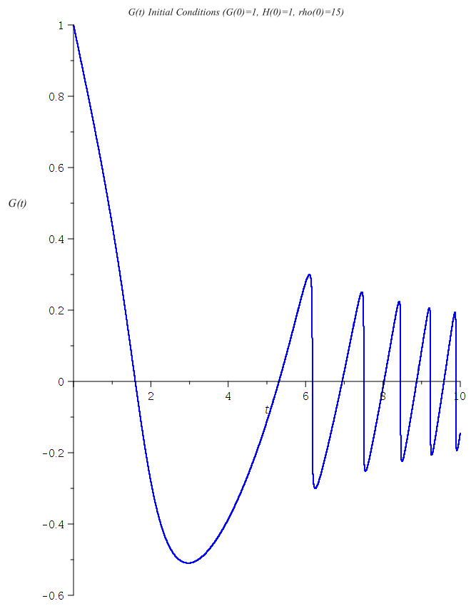
Figure 9: Plot of $\mathcal{G}(t)\times t$ for the Integral solution in the phase space $[\mathcal{G}\times H\times\rho_{m}]$ with initial condition $\mathcal{G}(0)=1$, $H(0)=1$, $\rho(0)=15$.

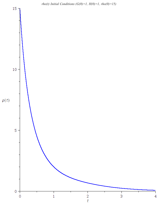
Figure 10: Plot of $\rho_{m}(t)\times t$ for the Integral solution in the phase space $[\mathcal{G}\times H\times\rho_{m}]$ with initial condition $\mathcal{G}(0)=1$, $H(0)=1$, $\rho(0)=15$.

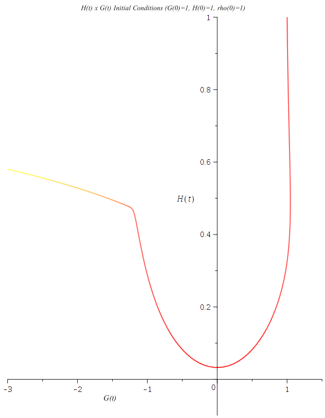
Figure 11: Plot of $\mathcal{G}(t)\times H(t)$ for the Integral solution in the phase space $[\mathcal{G}\times H\times\rho_{m}]$ with initial condition $\mathcal{G}(0)=1$, $H(0)=1$, $\rho(0)=1$.

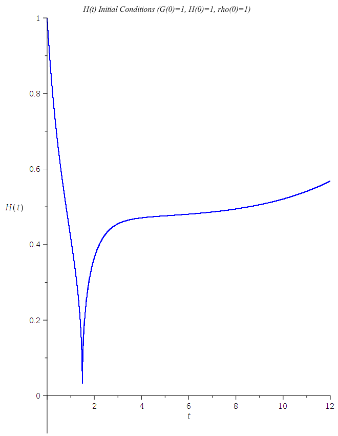
Figure 12: Plot of $H(t)\times t$ for the Integral solution in the phase space $[\mathcal{G}\times H\times\rho_{m}]$ with initial condition $\mathcal{G}(0)=1$, $H(0)=1$, $\rho(0)=1$. The $H(t)$ parameter has one minimum value.

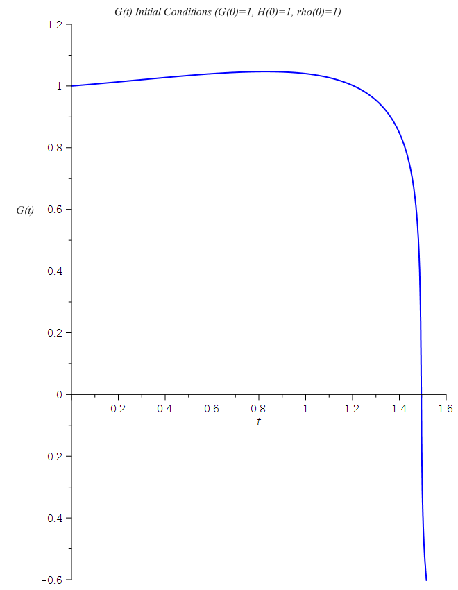
Figure 13: Plot of $\mathcal{G}(t)\times t$ for the Integral solution in the phase space $[\mathcal{G}\times H\times\rho_{m}]$ with initial condition $\mathcal{G}(0)=1$, $H(0)=1$, $\rho(0)=1$. $\mathcal{G}$ changes sign only one time.

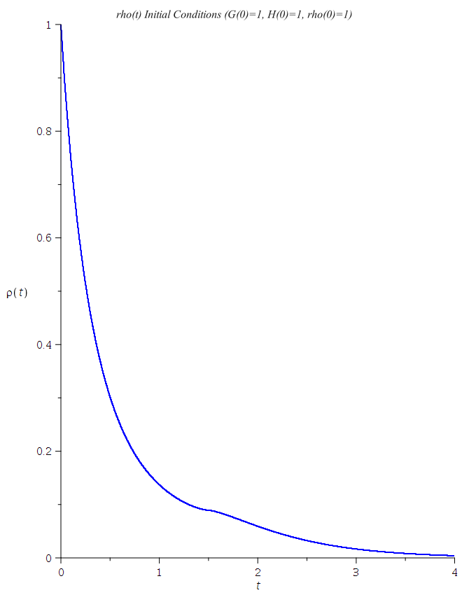
Figure 14: Plot of $\rho_{m}(t)\times t$ for the Integral solution in the phase space $[\mathcal{G}\times H\times\rho_{m}]$ with initial condition $\mathcal{G}(0)=1$, $H(0)=1$, $\rho(0)=1$.

V Conclusions

The rank-3 tensor representation of a spin-2 field appears directly in the modified equations of $f(\mathcal{G})$ gravity as a covariant divergent. In a homogeneous and isotropic Friedmann’s universe, if the geometric density $\rho_{Z}$ is strictly positive, then the topological invariant $\mathcal{G}$ can only be constant over a finite interval of time in order for the density mass $\rho_{m}$ to be strictly positive, this gives one necessary, but not a sufficient tool to filter out non-physical solutions.

The simplest non-trivial case we can consider, $f(\mathcal{G})=\sigma G^{2}$, gives rise to different behaviors for a Friedmann’s universe. In the empty space-time case, it can describe a universe that is always in accelerated expansion, or that is decelerated and accelerates at a later phase; or describe a universe that is expanding in phases of decreasing acceleration and deceleration. When cosmic dust is added to the system, its initial value will dictate how this universe will evolve, if it will expand with increasing dampened phases of acceleration and deceleration, or if it will expand with ever increasing acceleration.

The next natural step would be to compare the numerical solutions with real observational data to constrain the value of $\sigma$ and verify if it is reasonable. In our dynamical systems $\mathcal{G}$ was unbounded, it would be worthwhile to bound $\mathcal{G}$ to a finite interval using a Born-Infeld type function, summing or multiplying the original function, and verify how this boundary for $\mathcal{G}$, and its variation, would affect the evolution of the system.

References

- [1] David Lovelock. The einstein tensor and its generalizations. J. Math. Phys., 12(498), 1971.
- [2] S.D. Odintsov and S. Nojiri. Modified Gauss-Bonnet theory as gravitational alternative for dark energy. Physics Letters B, 631(1-2), 2005.
- [3] S.D. Odintsov and S. Nojiri. Introduction to modified gravity and gravitational alternative for dark energy. International Journal of Geometric Methods in Modern Physics, 4(01), 2007.
- [4] Ivan de Martino, Mariafelicia De Laurentis, and Salvatore Capozziello. Tracing the cosmic history by Gauss-Bonnet gravity. Physical Review D, 102(6):063508, September 2020.
- [5] S. D. Odintsov, S. Nojiri, and V. K. Oikonomou. Ghost-free Gauss-Bonnet theories of gravity. Physical Review D, 99(4), February 2019.
- [6] Dražen Glavan and Chunshan Lin. Einstein-Gauss-Bonnet gravity in 4-dimensional space-time. Physical Review Letters, 124(8):081301, February 2020.
- [7] Micol Benetti, Simony Santos da Costa, Salvatore Capozziello, Jailson S. Alcaniz, and Mariafelicia De Laurentis. Observational constraints on gauss–bonnet cosmology. International Journal of Modern Physics D, 27(08):1850084, may 2018.
- [8] Z. Molavi and A. Khodam-Mohammadi. Observational tests of Gauss-Bonnet like dark energy model. The European Physical Journal Plus, 134(6):254, June 2019.
- [9] S.D. Odintsov and V.K. Oikonomou. Inflationary phenomenology of einstein gauss-bonnet gravity compatible with gw170817. Physics Letters B, 797:134874, 2019.
- [10] Ugur Camci. On dark matter as a geometric effect in the galactic halo. Astrophysics and Space Science, 366(9), sep 2021.
- [11] S. Nojiri, S.D. Odintsov, and V.K. Oikonomou. Modified gravity theories on a nutshell: Inflation, bounce and late-time evolution. Physics Reports, 692:1–104, jun 2017.
- [12] R. Myrzakulov, L. Sebastiani, and S. Zebini. Some Aspects of Generalized Modified Gravity Models. International Journal of Modern Physics D, 22(08):1330017, jun 2013.
- [13] Konstantinos F. Dialektopoulos and Salvatore Capozziello. Noether symmetries as a geometric criterion to select theories of gravity. International Journal of Geometric Methods in Modern Physics, 15(supp01):1840007, nov 2018.
- [14] Pedro G S Fernandes, Pedro Carrilho, Timothy Clifton, and David J Mulryne. The 4d einstein–gauss–bonnet theory of gravity: a review. Classical and Quantum Gravity, 39(6):063001, feb 2022.
- [15] M Novello and Ronaldo Neves. Spin-2 field theory in curved spacetime in the Fierz representation. Classical and Quantum Gravity, 19:5335, October 2002.
- [16] Salvatore Capozziello, Carlo Alberto Mantica, and Luca Guido Molinari. Cosmological perfect fluids in gauss–bonnet gravity. International Journal of Geometric Methods in Modern Physics, 16(09):1950133, sep 2019.
- [17] Sebastian Bahamonde, Christian G. Böhmer, Sante Carloni, Edmund J. Copeland, Wei Fang, and Nicola Tamanini. Dynamical systems applied to cosmology: Dark energy and modified gravity. Physics Reports, 775-777:1–122, nov 2018.
- [18] Harvey Gould and Jan Tobochnik. An Introduction to Computer Simulation Methods: Applications to Physical Systems. Addison Wesley.