Conformal and nonminimal couplings in fractional cosmology

Abstract

Fractional differential calculus is a mathematical tool that has found applications in studying social and physical behaviours considered "anomalous". It is often used when traditional integer derivatives models fail to represent cases where the power law is observed accurately. Fractional calculus must reflect non-local, frequency- and history-dependent properties of power-law phenomena. This tool has various important applications, such as fractional mass conservation, electrochemical analysis, groundwater flow problems, and fractional spatiotemporal diffusion equations. It can also be used in cosmology to explain late-time cosmic acceleration without the need for dark energy. We review some models using fractional differential equations. We assume the Einstein-Hilbert action based on a fractional derivative action and add a scalar field $\phi$ to create a non-minimal interaction theory with the coupling $\xi R\phi^{2}$ between gravity and the scalar field, where $\xi$ is the interaction constant. By employing various mathematical approaches, we can offer precise schemes to find analytical and numerical approximations of the solutions. Moreover, we comprehensively study the modified cosmological equations and analyze the solution space using the theory of dynamical systems and asymptotic expansion methods. This enables us to provide a qualitative description of cosmologies with a scalar field based on fractional calculus formalism.

I Introduction

Fractional differential calculus is a mathematical tool that has found applications in studying social and physical behaviours considered "anomalous". These phenomena are often described empirically using the power law, which is universal. However, some of the mathematical models that use integer derivatives, including nonlinear models, need to work better in many cases where the power law is observed. Alternative tools like fractional calculus must be introduced to accurately reflect power-law phenomena’ non-local, frequency- and history-dependent properties.

Fractional calculus has found critical applications in areas such as fractional mass conservation. In such cases, a fractional mass conservation equation is needed to model fluid flow when the control volume is not large enough compared to the scale of heterogeneity and when the flow within the volume control is not linear. Other areas where fractional calculus is useful include electrochemical analysis and the problem of groundwater flow. In the latter, Darcy’s classical law is generalized by considering the water flow as a function of a non-integer order derivative of the piezometric height. This generalized law and the law of conservation of mass are then used to derive a new equation for groundwater flow.

Other examples of fractional calculus applications are the fractional advection-dispersion equation and fractional spatiotemporal diffusion equations. These models help characterize anomalous diffusion processes in complex media. An extension of the fractional derivative is the fractional derivative of variable order. This tool is helpful in structural damping models, where fractional derivatives are used to model viscoelastic damping in certain materials such as polymers. In quantum theory, some important examples of fractional calculus are the fractional Schrödinger equation and versions such as the variable order fractional Schrödinger equation. Recent studies have also demonstrated the usefulness of fractional calculus in cosmology. Modifying the theory using fractional calculus explains late-time cosmic acceleration without including dark energy.

I.1 Research questions

• Is it possible to use a combination of local and global variables to qualitatively describe scalar field cosmologies based on the fractional calculus formalism?

• Is it possible to provide precise schemes for finding analytical and numerical approximations to solutions by choosing various approaches?

I.2 Problem Statement

A formulation of gravity with a scalar field that shows non-minimal or conformal coupling to gravity is presented. The new action includes the Ricci scalar $R$, the scalar field $\phi$ with its potential $V(\phi)$, the coupling constant $\xi$, the matter Lagrangian $L_{m}$, the scale factor $a$, and the lapse function $N$. The Gamma function $\Gamma(\mu)$, the fractional parameter $\mu$, and the equation of state parameter of matter $w$ are also included. A comprehensive review of the state of the art has been conducted, and it has been confirmed that dynamical systems theory, methods of perturbation theory, and the main tools of fractional calculus can be combined to implement qualitative analysis of gravity models with fractional derivatives. That is especially useful in cosmologies with scalar fields and conformal coupling and non-minimal coupling to gravity, thereby generalizing previous results.

I.3 Goals

I.3.1 General Objective

• The general objective of this paper is to analyze new and known results from cosmologies with scalar fields and gravity models with fractional derivatives, especially for a scalar field with conformal coupling and non-minimal coupling to gravity.

I.3.2 Specific Objectives

1. Explore the role of dynamical systems theory and the tools of fractional calculus in the analysis of cosmological models.

2. Propose cosmologies with scalar fields with conformal and non-minimal coupling to gravity in fractional calculus.

3. Qualitative analysis of models using dynamical systems and asymptotic methods to expand our understanding and allow comprehensive conclusions.

I.4 Research hypotheses

After conducting a thorough literature review and developing a theoretical framework, a research hypothesis has been formulated that proposes the possibility of obtaining relevant information on the flow properties associated with an autonomous system of ordinary differential equations in the cosmological context through qualitative techniques. The dynamical systems theory enables us to provide qualitative descriptions of cosmologies with a scalar field in fractional calculus. Moreover, it is possible to offer schemes for finding analytical approximations of solutions and exact solutions by selecting various approaches.

I.5 Methodology

Our methodology first involves reviewing the literature on fractional calculus methods, solution of fractional differential equations, and their applications. The current literature on applying fractional differential calculus to theories of gravity will also be studied, obtaining modifications. The differential equations that describe the dynamics of the different models are to be derived and well-posed for mathematical analysis and physical interpretation. At this point, it is expected to select the work tools and become familiar with Caputo’s fractional derivative and its application in formulating a fractional cosmological action and its respective variational calculation. Secondly, systems of ordinary differential equations will be derived and analyzed from a mathematical point of view. This analysis consists of several steps: finding equilibrium points and invariant sets; defining a linearization matrix for each system and evaluating it at each critical point to calculate the eigenvalues; classifying the stability of the points; generating phase space diagrams and numerical solutions for each system for appropriate values of the coupling and fractional parameters. It is expected to find each system’s future and past attractors and classify each critical point according to its stability and asymptotic behaviour. The dynamical behaviour of the systems will also be described graphically by plotting orbits that illustrate the qualitative analysis, which allows the description of the cosmological evolution. Finally, we generalize previous results by considering a conformal and non-minimal coupling to gravity.

I.6 Scientific Novelty

We consider corrections of the Friedmann and Klein-Gordon equations using Caputo’s derivative and the formalism of fractional calculus. This approach offers a high level of applicability to describe natural phenomena, making it a novel and attractive scenario.

In the fractional context, we analyze cosmologies with a scalar field coupled to gravity with conformal and non-minimal coupling. We aim to generalize previous results within the framework of the fractional formulation of gravity and describe the phase space of the models. We obtain qualitative results and explicit and approximate exact solutions with high numerical precision from a mathematical point of view.

I.7 Organization

The paper is organized as follows. Section II covers the main outcomes of fractional calculus, including different approaches to possible fractional derivatives such as Grünwald-Letnikov, Riemann-Liouville, and Caputo derivatives. The emphasis is on defining fractional integration and the fractional derivative. We also discuss fractional differential equations and use Wolfram Language 13.3 (Wolfram Research,, 2023) to solve physical problems formulated.

In section III, we explore fractional cosmologies with non-minimal coupling ($\xi\neq 0$), building upon previous results with minimal coupling. By studying different dynamical systems, including the invariant set $\Omega_{\Lambda}=0$, we utilized numerical integration methods to analyze the behaviour of solutions to differential equations from the cosmological model. We also investigated the stability of critical points. Conclusions are given in section IV. In appendix A, we define several special functions that appear recurrently in these topics.

II Theoretical Framework

Fractional calculus is a field of study that deals with the extension of derivatives and integrals to fractional orders. It also focuses on the methods for solving differential equations that involve these fractional derivatives and fractional integrals. It was developed by Newton and Leibniz in the 17th century and involves two fundamental operations - differentiation and integration. These fractional operators have memory and are more flexible when describing the dynamic behaviour of phenomena and systems using fractional differential equations. On the other hand, the description with integer differential equations uses local operators and is limited in the differentiation order to a constant. Consequently, the resulting models must be sufficiently accurate in many cases West, (2021).

Although many contributions have been made to this topic over the years, it has not been applied directly for centuries. However, in recent years, its applications have grown tremendously, and it is now used universally as an empirical description of complex social and physical phenomena. Research on fractional differentiation spans multiple disciplines and has various applications, such as fractional spacetime in quantum mechanics and gravity and fractional quantum field theory (Calcagni, 2010b, ; Calcagni, 2010a, ; Lim,, 2006; Lim and Eab,, 2019; V. Moniz and Jalalzadeh,, 2020; Moniz and Jalalzadeh,, 2020; Rasouli et al.,, 2021; Jalalzadeh et al.,, 2021). By utilizing these frameworks, researchers have been able to gain a better understanding of complex systems in classical and quantum regimes  (Rami,, 2009; El-Nabulsi,, 2009, 2010, 2011, 2012; El-Nabulsi and Wu,, 2012; El-Nabulsi, 2013a, ; El-Nabulsi,, 2015; El-Nabulsi, 2016a, ; El-Nabulsi,, 2018, 2020). This branch of mathematics is gaining more popularity in fluid dynamics, control theory, and signal processing. Due to the importance and potential of this topic, support for fractional derivatives and fractional integrals has been added to the Wolfram Language since the release of Version 13.1 https://blog.wolfram.com/2022/08/12/fractional-calculus-in-wolfram-language-13-1/ (revised on February 20th, 2024). This paper will be using Wolfram Language 13.3 (Wolfram Research,, 2023).

Niels Henrik Abel is known for contributing to fractional calculus in the early 19th century. He introduced the integration and differentiation of fractional order and their inverse relationship. Abel also unified the notation for differentiation and integration of arbitrary real order in the "differintegral" operation. Abel considered the generalized version of the tautochrone problem; formulated as the integral equation

$$f(x)=\int_{0}^{x}\frac{\phi(s)}{\sqrt{x-s}}\,ds,$$ (1)

for the unknown function $\phi(x)$. After several algebraic manipulations, this integral equation could be rewritten in the form

$$\phi(x)=\frac{1}{\pi}\left(\frac{f(0)}{\sqrt{x}}+\int_{0}^{x}\frac{f^{\prime}(\tau)}{\sqrt{x-\tau}}\,d\tau\right),$$ (2)

which is what we now call Caputo’s fractional derivative of $f(x)$ with respect to $x$.

Scientists from various areas and backgrounds have been working on fractional calculus theory, approaching it from different perspectives. Some approaches define a fractional differentiation operation. In contrast, others consider a unified differentiation/integration operation, known as the fractional differintegral of order $\mu$, with respect to $x$ and a lower limit $a$. Differintegrals depend on the function’s value at point $a$, $f(a)$, using the function’s "history". In practice, the lower limit is generally taken as 0.

Summarizing, in fractional calculus, the traditional derivatives and integrals of integer order have been generalized to derivatives and integrals of arbitrary order. This concept is presented in various sources, including  (Podlubny,, 1998; Kilbas et al.,, 2006; Monje et al.,, 2010; Klafter et al.,, 2012; Tarasov,, 2013; Uchaikin,, 2013; Bandyopadhyay and Kamal,, 2014; Padula and Visioli,, 2014; Herrmann,, 2014; Malinowska et al.,, 2015; Lorenzo and Hartley,, 2016; Tarasov,, 2019). The idea is that a derivative operator of order $n$, which is a natural number, has been generalized to a derivative of order $\mu$, which can be a complex number or even a complex function. The three most popular and influential definitions widely used in practice are the Grünwald-Letnikov differintegral, the Riemann–Liouville fractional derivative and Caputo’s fractional derivative.

II.1 Grünwald–Letnikov Approach

The Grünwald-Letnikov differintegral provides the basic extension of classical derivatives/integrals and is based on limits:

$${}_{0}D_{x}^{\mu}f(x)=\lim_{h\rightarrow 0}h^{-\mu}\sum_{r=0}^{\infty}(-1)^{r}\begin{pmatrix}\mu\\ r\end{pmatrix}f(x-rh).$$ (3)

In practice, this approach is useless since it contains infinite approximations of the function at different points.

II.2 Riemann–Liouville approach

The definition of the Riemann–Liouville fractional derivative is:

$${}^{\text{RL}}_{0}{D}_{x}^{\mu}f(x)=\frac{1}{\Gamma(n-\mu)}\frac{d^{n}}{dx^{n}}\left(\int_{0}^{x}(x-\tau)^{n-\mu-1}f(\tau)d\tau\right),$$ (4)

where $n=\max\{0,\lfloor\mu\rfloor\}$, where $\lfloor x\rfloor$ denotes the floor function, $\lfloor x\rfloor=\max\{m\in\mathbb{Z}:m\leq x\}$.

It is based on a solid and strict mathematical theory of fractional calculus. This theory is well developed, but the Riemann-Liouville approach has some limitations that make it less suitable for applications in real-world problems.

For example, the derivative of a constant is not zero:

$${}^{\text{RL}}_{0}D_{x}^{\mu}\text{constant}=\frac{\text{constant}}{\Gamma(1-\mu)}x^{-\mu}.$$ (5)

Table 1: The $\mu$-th fractional derivatives of Riemann-Liouville and $n$-th ordinary derivatives for some common functions.

$f(x)$	$D^{\mu}_{x}(f(x))$	$f^{(n)}(x)$
$e^{x}$	$-e^{x}\left(Q(-\mu,x)-1\right)$	$e^{x}$
$x^{2}$	$\frac{2x^{2-\mu}}{\Gamma(3-\mu)}$	$\frac{2x^{2-n}}{(2-n)!}$
$\log(x)$	$\left\{\begin{array}[]{cc}-(-1)^{\mu}(\mu-1)!x^{-\mu}&\mu\in\mathbb{Z}\land\mu>0\\ -\frac{x^{-\mu}\left(\psi^{(0)}(1-\mu)-\log(x)+\gamma\right)}{\Gamma(1-\mu)}&\text{True}\end{array}\right.$	$\left\{\begin{array}[]{cc}-(-1)^{n}(n-1)!x^{-n}&n\geq 1\\ \log(x)&\text{True}\end{array}\right.$
$\sin(x)$	$\sqrt{\pi}\,2^{\mu-1}x^{1-\mu}\,{}_{1}\tilde{F}_{2}\left(1;1-\frac{\mu}{2},\frac{3-\mu}{2};-\frac{x^{2}}{4}\right)$	$\sin\left(\frac{\pi n}{2}+x\right)$
$\tan^{-1}(x)$	$\sqrt{\pi}\,2^{\mu-1}x^{1-\mu}\,{}_{3}\tilde{F}_{2}\left(\frac{1}{2},1,1;1-\frac{\mu}{2},\frac{3-\mu}{2};-x^{2}\right)$	$\sqrt{\pi}\,2^{n-1}x^{1-n}\,{}_{3}\tilde{F}_{2}\left(\frac{1}{2},1,1;1-\frac{n}{2},\frac{3-n}{2};-x^{2}\right)$
$J_{0}(x)$	$\sqrt{\pi}\,2^{\mu}x^{-\mu}\,{}_{1}\tilde{F}_{2}\left(\frac{1}{2};\frac{1-\mu}{2},1-\frac{\mu}{2};-\frac{x^{2}}{4}\right)$	$2^{-n}\sum_{K_{1}=0}^{n}(-1)^{K_{1}}J_{2K_{1}-n}(x)\begin{pmatrix}n\\ K_{1}\end{pmatrix}$
${}_{1}F_{1}(a;b;x)$	$\Gamma(b)x^{-\mu}{}_{2}\tilde{F}_{2}\left(1,a;1-\mu,b;x\right)$	$\left\{\begin{array}[]{cc}\Gamma(b)x^{-n}{}_{2}\tilde{F}_{2}\left(1,a;1-n,b;x\right)&n\geq 1\\ {}_{1}F_{1}(a;b;x)&\text{True}\end{array}\right.$

Table 1 shows the $\mu$-th fractional derivatives and $n$-th ordinary derivatives for some standard functions (see appendix A for definitions of special functions).

II.2.1 Caputo’s Approach

Caputo’s definition of fractional derivative is:

$${}^{\text{C}}_{0}{D}_{x}^{\mu}f(x)=\frac{1}{\Gamma(n-\mu)}\int_{0}^{x}(x-\tau)^{n-\mu-1}\frac{d^{n}}{d\tau^{n}}f(\tau)d\tau,\quad n=\left\{\begin{array}[]{cc}\lfloor\mu\rfloor+1&\mu\notin\mathbb{N}\\ \mu&\mu\in\mathbb{N}\end{array}\right..$$ (6)

There is some similarity between this and the Riemann-Liouville differintegral, and in fact, the Caputo differintegral can be defined via the Riemann-Liouville differintegral by:

$${}^{\text{C}}_{0}{D}_{x}^{\mu}f(x)={}^{RL}_{0}D_{x}^{\mu}-\sum_{k=0}^{\lfloor\mu\rfloor-1}\frac{x^{k-\mu}}{\Gamma(k-\mu+1)}\frac{d^{k}}{dx^{k}}f(0).$$ (7)

Caputo’s definition of fractional and integral derivatives has many advantages compared to those of Riemann-Liouville or Grünwald-Letnikov: first, it takes into account the values of the function and its derivatives at the origin (or, in general, at any lower or upper bound $a$), which automatically makes it suitable for solving fractional order initial value problems using Laplace transforms. Furthermore, the Caputo fractional derivative of a constant is $0$. Therefore, it is more consistent with the classical calculation.

The Riemann-Liouville fractional differintintegral has been implemented in the Wolfram Language, using the Wolfram Language Version 13.3 (Wolfram Research,, 2023) function FractionalD. This function calculates the Riemann-Liouville fractional derivative of order $\mu$ of the function $f(x)$; the lower limit of the integral is considered $0$.

The Caputo fractional differential integral is CaputoD in Wolfram Language 13.1, which gives the Caputo fractional derivative of order $\mu$ of a function $f(x)$. For negative orders of $\mu$, the output of CaputoD matches FractionalD.

Table 2: Half-order Caputo fractional derivatives of some common mathematical functions.

$f(x)$	$D^{\frac{1}{2}}_{x}(f(x))$
$e^{x}$	$e^{x}\text{erf}(\sqrt{x})$
$x^{2}$	$\frac{8x^{\frac{3}{2}}}{3\sqrt{\pi}}$
$\log(x)$	$\frac{\log(4)}{\sqrt{\pi}\sqrt{x}}$
$\sin(x)$	$\frac{2\sqrt{x}\;{}_{1}F_{2}\left(1;\frac{3}{4},\frac{5}{4};-\frac{x^{2}}{4}\right)}{\sqrt{\pi}}$
$\tan^{-1}(x)$	$\frac{2\sqrt{x}\;{}_{2}F_{3}\left(\frac{1}{2},1,1;\frac{3}{4},\frac{5}{4};-x^{2}\right)}{\sqrt{\pi}}$
$J_{0}(x)$	$\frac{{}_{1}F_{2}\left(\frac{1}{2};\frac{1}{4},\frac{3}{4};-\frac{x^{2}}{4}\right)-1}{\sqrt{\pi}\sqrt{x}}$
${}_{1}F_{1}(a;b;x)$	$\frac{{}_{2}F_{2}\left(1,a;\frac{1}{2},b;x\right)-1}{\sqrt{\pi}\sqrt{x}}$

Table 2 presents the half-order Caputo fractional derivatives of some common mathematical functions.

II.2.2 Chain rule for fractional derivatives

The Caputo fractional derivative for an arbitrary $c$ is (Malinowska et al.,, 2015)

$${}^{\text{C}}_{c}D_{x}^{\mu}f(t)=\frac{1}{\Gamma(n-\mu)}\int_{c}^{x}\frac{d^{n}f(\tau)}{d\tau^{n}}\left(x-\tau\right)^{n-\mu-1}d\tau,\quad n=\left\{\begin{array}[]{cc}\lfloor\mu\rfloor+1&\mu\notin\mathbb{N}\\ \mu&\mu\in\mathbb{N}\end{array}\right..$$ (8)

Given the square function: $f(x)=x^{2}/2$, choosing $c=0$, and removing the subindex $0$, and applying the derivative of order $1/2$ twice, it results: $\mu=1/2\Rightarrow n:=\lfloor\mu\rfloor+1=1$,

$${}^{\text{C}}D_{x}^{1/2}\left(x^{2}/2\right)=\frac{1}{\Gamma(\frac{1}{2})}\int_{0}^{x}\frac{d}{dt}\left[\frac{t^{2}}{2}\right](x-t)^{-\frac{1}{2}}dt=\frac{1}{\sqrt{\pi}}\frac{4}{3}x^{\frac{3}{2}},$$

$${}^{\text{C}}D_{x}^{1/2}\left(\frac{1}{\sqrt{\pi}}\frac{4}{3}x^{\frac{3}{2}}\right)=\frac{1}{\sqrt{\pi}}\frac{4}{3}\frac{1}{\Gamma(\frac{1}{2})}\int_{0}^{x}\frac{d}{dt}\left[t^{\frac{3}{2}}\right](x-t)^{-\frac{1}{2}}dt=\frac{1}{\sqrt{\pi}}\frac{4}{3}\frac{1}{\sqrt{\pi}}\frac{3\pi x}{4}=x.$$

The first derivative of the square function is obtained through two "half-order fractional differentiation" procedures. One could easily verify that the antiderivative of the square function can be obtained by two similar half-order integration procedures. So, with this example, we show what fractional calculus is and how it relates to and generalizes the classical version. However, this result holds because of the choice $c=0$. In general, the chain rule for fractional calculus is:

$$D_{x}^{\mu}\left[D_{x}^{\beta}f(x)\right]=D_{x}^{\mu+\beta}f(x)-\sum_{j=1}^{n}D_{x}^{\beta-j}f(c_{+})\frac{(x-c)^{-\mu-j}}{\Gamma(1-\mu-j)}.$$ (9)

II.2.3 Fractional derivatives as generalizations of integer order derivatives

From now on, we follow the book (Herrmann,, 2014). We have the formulas for the $n$-th derivatives,

$$\frac{d^{n}}{dx^{n}}e^{kx}=k^{n}e^{kx},\quad\frac{d^{n}}{dx^{n}}\sin{(kx)}=k^{n}\sin{\left(kx+\frac{\pi}{2}n\right)},\quad\frac{d^{n}}{dx^{n}}x^{k}=\frac{k!}{(k-n)!}x^{k-n},$$ (10)

for $n\in\mathbb{N}$ can be extended for real and complex $\mu$ numbers,

$$D_{x}^{\mu}e^{kx}=k^{\mu}e^{kx},\hskip 20.075ptk\geq 0,$$ (11)

$$D_{x}^{\mu}\sin{(kx)}=k^{\mu}\sin{\left(kx+\frac{\pi}{2}\mu\right)},\hskip 20.075ptk\geq 0,$$ (12)

$$D_{x}^{\mu}x^{k}=\frac{\Gamma(k+1)}{\Gamma(k+1-\mu)}x^{k-\mu},\hskip 20.075ptx\geq 0,k\neq-1,-2,-3,\ldots\hskip 5.01874pt.$$ (13)

The definition of the fractional derivative of the exponential function was given by Liouville in 1832; those of trigonometric functions were proposed by Fourier in 1822, and those of powers were systematically studied by Riemann in 1847. Still, the first attempts at the latter are due to Leibniz and Euler, the latter in 1738. The Riemann-Liouville fractional derivative of a constant is given by (13) setting $k=0$, we obtain unexpected behaviour

$$D_{x}^{\mu}1=D_{x}^{\mu}x^{0}=\frac{1}{\Gamma(1-\mu)}x^{-\mu}.$$

Therefore, as an additional postulate, Caputo in 1967 introduced the condition $D_{x}^{\mu}1=0$.

These four definitions of fractional derivative (11), (12), (13) and Caputo’s share several aspects. On the one hand, they satisfy the correspondence principle:

$$\lim_{\mu\to n}D_{x}^{\mu}f(x)=\frac{d^{n}}{dx^{n}}f(x),\hskip 10.03749ptn=0,1,2,\ldots\hskip 5.01874pt.$$ (14)

And also the following rules:

$$D_{x}^{\mu}cf(x)=cD_{x}^{\mu}f(x),\quad D_{x}^{\mu}[f(x)+g(x)]=D_{x}^{\mu}f(x)+D_{x}^{\mu}g(x).$$ (15)

Therefore, the fractional derivative of an analytic function can be calculated to its series.

According to Liouville:

$$f(x)=\sum_{k=0}^{\infty}a_{k}e^{kx}\implies D_{x}^{\mu}f(x)=\sum_{k=0}^{\infty}a_{k}k^{\mu}e^{kx}.$$ (16)

According to Fourier:

$$f(x)=a_{0}+\sum_{k=1}^{\infty}a_{k}\sin{(kx)}+\sum_{k=1}^{\infty}b_{k}\cos{(kx)},$$ (17)

$$D_{x}^{\mu}f(x)=\sum_{k=1}^{\infty}a_{k}k^{\mu}\sin{\left(kx+\frac{\pi}{2}\mu\right)}+\sum_{k=1}^{\infty}b_{k}k^{\mu}\cos{\left(kx+\frac{\pi}{2}\mu\right)}.$$ (18)

According to Riemann:

$$f(x)=x^{\mu-1}\sum_{k=0}^{\infty}a_{k}x^{k\mu},$$ (19)

$$D_{x}^{\mu}f(x)=x^{\mu-1}\sum_{k=0}^{\infty}a_{k+1}\frac{\Gamma((k+2)\mu)}{\Gamma((k+1)\mu)}x^{k\mu}.$$ (20)

According to Caputo

$$f(x)=\sum_{k=0}^{\infty}a_{k}x^{k\mu},$$ (21)

$$D_{x}^{\mu}f(x)=\sum_{k=0}^{\infty}a_{k+1}\frac{\Gamma(1+(k+1)\mu)}{\Gamma(1+k\mu)}x^{k\mu}.$$ (22)

Calculating the Caputo fractional derivative of order $\mu$ to the exponential function, we have

$$D_{x}^{\mu}e^{x}=D_{x}^{\mu}\sum_{n=0}^{\infty}\frac{x^{n}}{n!}=\sum_{n=1}^{\infty}\frac{x^{n-\mu}}{\Gamma(1+n-\mu)}=x^{1-\mu}E(1,2-\mu,x).$$ (23)

So, in contrast to Liouville’s definition (16), Caputo’s definition is not obviously in terms of an exponential, but in terms of a generalized Mittag-Leffler function (272).

II.2.4 Leibniz’s rule for the fractional derivative of the product

Let us now analyze whether all the techniques of ordinary differential calculus can be transferred to the field of fractional calculus (Herrmann,, 2014). For example, if we take the ordinary Leibniz rule:

$$\frac{d}{dx}(\psi\chi)=\left(\frac{d}{dx}\psi\right)\chi+\psi\left(\frac{d}{dx}\chi\right),$$ (24)

it could be carelessly inferred that the relation

$$D_{x}^{\mu}(\psi\chi)=\left(D_{x}^{\mu}\psi\right)\chi+\psi\left(D_{x}^{\mu}\chi\right),$$ (25)

remains in the fractional calculus. However, using Liouville’s definition of a fractional derivative, we have

$$D_{x}^{\mu}(e^{k_{1}x}e^{k_{2}x})=D_{x}^{\mu}e^{(k_{1}+k_{2})x}=(k_{1}+k_{2})^{\mu}e^{(k_{1}+k_{2})x}.$$ (26)

While using (25), we obtain

$$D_{x}^{\mu}(e^{k_{1}x}e^{k_{2}x})=(k_{1}^{\mu}+k_{2}^{\mu})(e^{k_{1}x}e^{k_{2}x}).$$ (27)

Therefore, Leibniz’s rule (25) is not valid for fractional derivatives.

We start from the rule for successive non-negative integer orders to extend Leibniz’s rule to be valid for fractional calculus.

$$\begin{split}&\frac{d}{dx}(\psi\chi)=\left(\frac{d}{dx}\psi\right)\chi+\psi\left(\frac{d}{dx}\chi\right),\\ &\frac{d^{2}}{dx^{2}}(\psi\chi)=\left(\frac{d^{2}}{dx^{2}}\psi\right)\chi+2\left(\frac{d}{dx}\psi\right)\left(\frac{d}{dx}\chi\right)+\psi\left(\frac{d^{2}}{dx^{2}}\chi\right),\\ &\frac{d^{3}}{dx^{3}}(\psi\chi)=\left(\frac{d^{3}}{dx^{3}}\psi\right)\chi+3\left(\frac{d^{2}}{dx^{2}}\psi\right)\left(\frac{d}{dx}\chi\right)+3\left(\frac{d}{dx}\psi\right)\left(\frac{d^{2}}{dx^{2}}\chi\right)+\psi\left(\frac{d^{3}}{dx^{3}}\chi\right),\end{split}$$ (28)

etcetera. We have the following formula for an arbitrary integer,

$$\frac{d^{n}}{dx^{n}}(\psi\chi)=\sum_{j=0}^{n}\begin{pmatrix}n\\ j\end{pmatrix}\left(\frac{d^{n-j}}{dx^{n-j}}\psi\right)\left(\frac{d^{j}}{dx^{j}}\chi\right),\hskip 20.075ptn\in\mathbb{N}.$$ (29)

According to (263), this expression can be extended to an arbitrary $\mu$:

$$D_{x}^{\mu}(\psi\chi)=\sum_{j=0}^{\infty}\frac{\Gamma(\mu+1)}{\Gamma(j+1)\Gamma(\mu-j+1)}(D_{x}^{\mu-j}\psi)(D_{x}^{j}\chi),$$ (30)

So, this form of Leibniz’s product derivative rule is also valid for fractional derivatives.

II.3 Fractional integral

The Cauchy formula for successive integrations, which can be extended to fractional integrals, is used as a first step. A satisfactory definition of a fractional derivative can be obtained after appropriately deriving a fractional integral $I^{\mu}$. If it is assumed

$$D_{x}^{\mu}=I^{-\mu},$$ (31)

which is equivalent to requiring that a fractional derivative is the inverse of a fractional integral and vice versa; a fractional integral is the inverse of a fractional derivative.

If ${}_{a}{I}$ is used for the integration operator

$${}_{a}{I}f(x)=\int_{a}^{x}f(\xi)\,d\xi,$$ (32)

It is observed that the multiple integral is

$${}_{a}{I^{n}}f(x)=\int_{a}^{x}\int_{a}^{x_{n-1}}\cdots\int_{a}^{x_{1}}f(x_{0})\,dx_{0}\dotsb dx_{n-1},$$ (33)

which, using Cauchy’s repeated integration formula, can be reduced to a single integral:

$${}_{a}{I^{n}}f(x)=\frac{1}{(n-1)!}\int_{a}^{x}(x-\xi)^{n-1}f(\xi)\,d\xi.$$ (34)

This formula can be easily extended to the fractional case:

$${}_{a}{I_{+}^{\mu}}f(x)=\frac{1}{\Gamma(\mu)}\int_{a}^{x}(x-\xi)^{\mu-1}f(\xi)\,d\xi,\hskip 20.075ptx>a,$$ (35)

$${}_{b}{I_{-}^{\mu}}f(x)=\frac{1}{\Gamma(\mu)}\int_{x}^{b}(\xi-x)^{\mu-1}f(\xi)\,d\xi,\hskip 20.075ptx<b.$$ (36)

The constants $a$ and $b$ determine the lower and upper limits of the integral, respectively, and can initially be chosen arbitrarily. The two cases are called the left and right, respectively. That can be understood because the left case deals with values $\xi<x$, values to the left of $x$. The right case deals with values $\xi>x$, values to the right of $x$. If $x$ is a time-type coordinate, then the integral of the left case is causal, and that of the right case is anti-causal.

The value of the integral depends on the specific choice of the constants $(a,b)$. That will be the notable difference between the two most widely used definitions of a fractional integral, the so-called Liouville fractional integral and the Riemann fractional integral, which are discussed below.

II.3.1 Liouville fractional integral

The Liouville fractional integral is defined by making $a=-\infty$ and $b=+\infty$ in (35) and (36):

$${}_{\text{L}}{I_{+}^{\mu}}f(x)=\frac{1}{\Gamma(\mu)}\int_{-\infty}^{x}(x-\xi)^{\mu-1}f(\xi)\,d\xi,$$ (37)

$${}_{\text{L}}{I_{-}^{\mu}}f(x)=\frac{1}{\Gamma(\mu)}\int_{x}^{+\infty}(\xi-x)^{\mu-1}f(\xi)\,d\xi.$$ (38)

II.3.2 Riemann Fractional Integral

The fractional Riemann integral is defined by making $a=0$ and $b=0$ in (35) and (36):

$${}_{\text{R}}{I_{+}^{\mu}}f(x)=\frac{1}{\Gamma(\mu)}\int_{0}^{x}(x-\xi)^{\mu-1}f(\xi)\,d\xi,$$ (39)

$${}_{\text{R}}{I_{-}^{\mu}}f(x)=\frac{1}{\Gamma(\mu)}\int_{x}^{0}(\xi-x)^{\mu-1}f(\xi)\,d\xi.$$ (40)

To see the difference between Liouville’s definition (37), (38) and Riemann’s definition (39), (40) apply both definitions to $f(x)=e^{kx}$:

$${}_{\text{L}}{I_{+}^{\mu}}e^{kx}=k^{-\mu}e^{kx},x>0,\quad_{\text{L}}{I_{-}^{\mu}}e^{kx}=(-k)^{-\mu}e^{kx},k<0,$$

$${}_{\text{R}}{I_{+}^{\mu}}e^{kx}=k^{-\mu}e^{kx}\left(1-\frac{\Gamma(\mu,kx)}{\Gamma(\mu)}\right),x>0,\quad_{\text{R}}{I_{-}^{\mu}}e^{kx}=(-k)^{-\mu}e^{kx}\left(1-\frac{\Gamma(\mu,kx)}{\Gamma(\mu)}\right),x<0,$$

where $\Gamma(\mu,x)$ is the incomplete Gamma function. Using Liouville’s definition, the function $e^{kx}$ vanishes for $k>0$ in the lower limit of the domain of the integral, so there is no additional contribution. On the other hand, when using the Riemann definition, an additional contribution is obtained because, at $a=0$, the exponential function does not vanish (Herrmann,, 2014).

II.4 Link between integration and fractional differentiation

Using the abbreviation

$$D_{x}^{\mu}=D^{\mu},$$ (41)

It is shown that the concepts of fractional integration and fractional differentiation are closely related. Separating the fractional derivative operator into factors,

$$D^{\mu}=D^{m}D^{\mu-m}=\frac{d^{m}}{dx^{m}}_{a}{I^{m-\mu}},\hskip 20.075ptm\in\mathbb{N}.$$ (42)

A fractional derivative can be interpreted as a fractional integral followed by an ordinary derivative. Once the fractional integral is specified, the fractional derivative is automatically determined. We can also reverse the sequence of the operators, resulting in an alternative decomposition:

$$D^{\mu}=D^{\mu-m}D^{m}=_{a}{I^{m-\mu}}\frac{d^{m}}{dx^{m}},\hskip 20.075ptm\in\mathbb{N}.$$ (43)

The decompositions (42) and (43) lead to different results. Thus, we can understand the mechanism by which non-locality enters fractional calculus. The standard derivative, of course, is a local operator, but the fractional integral certainly is not. The fractional derivative should be understood as the inverse of fractional integration, a non-local operation. Consequently, fractional differentiation and integration produce the same difficulty (Herrmann,, 2014).

In the previous section, two different definitions of the fractional integral have been given, the Liouville and the Riemann. For each of these definitions, according to the two different decompositions given above, four different realizations follow for the definition of fractional derivative, which are presented below.

II.4.1 Liouville fractional derivative

For the simple case $0<\mu<1$, using the Liouville definition (37) and (38), and the sequence of operators (42), we have

$${}_{\text{L}}{D_{+}^{\mu}}f(x)=\frac{d}{dx}_{\text{L}}{I_{+}^{1-\mu}}f(x)=\frac{1}{\Gamma(1-\mu)}\frac{d}{dx}\int_{-\infty}^{x}(x-\xi)^{-\mu}f(\xi)\,d\xi,$$ (44)

$${}_{\text{L}}{D_{-}^{\mu}}f(x)=\frac{d}{dx}_{\text{L}}{I_{-}^{1-\mu}}f(x)=\frac{1}{\Gamma(1-\mu)}\frac{d}{dx}\int_{x}^{+\infty}(\xi-x)^{-\mu}f(\xi)\,d\xi.$$ (45)

II.4.2 Fractional Riemann derivative

Using (39), (40) and the sequence of operators (42), we have the Riemann fractional derivative:

$${}_{\text{R}}{D_{+}^{\mu}}f(x)=\frac{d}{dx}_{\text{R}}{I_{+}^{1-\mu}}f(x)=\frac{1}{\Gamma(1-\mu)}\frac{d}{dx}\int_{0}^{x}(x-\xi)^{-\mu}f(\xi)\,d\xi,$$ (46)

$${}_{\text{R}}{D_{-}^{\mu}}f(x)=\frac{d}{dx}_{\text{R}}{I_{-}^{1-\mu}}f(x)=\frac{1}{\Gamma(1-\mu)}\frac{d}{dx}\int_{x}^{0}(\xi-x)^{-\mu}f(\xi)\,d\xi.$$ (47)

II.4.3 Liouville-Caputo fractional derivative

In the case that the sequence of operators is inverted according to (43), it is based on the definition of Liouville fractional integral (37) and (38):

$${}_{\text{LC}}{D_{+}^{\mu}}f(x)=_{\text{L}}{I_{+}^{1-\mu}}\frac{d}{dx}f(x)=\frac{1}{\Gamma(1-\mu)}\int_{-\infty}^{x}(x-\xi)^{-\mu}\frac{df(\xi)}{d\xi}\,d\xi,$$ (48)

$${}_{\text{LC}}{D_{-}^{\mu}}f(x)=_{\text{L}}{I_{-}^{1-\mu}}\frac{d}{dx}f(x)=\frac{1}{\Gamma(1-\mu)}\int_{x}^{+\infty}(\xi-x)^{-\mu}\frac{df(\xi)}{d\xi}\,d\xi.$$ (49)

It is observed that for a function $f(x)=$ constant, the definition of the Liouville fractional derivative (44) leads to a divergent result, while with the Liouville-Caputo definition (48), the result is zero. The conditions for the Liouville fractional derivative to converge are more restrictive than for the Liouville-Caputo counterpart (Herrmann,, 2014).

II.4.4 Caputo fractional derivative

The inverted sequence of operators (43), the definition of the Riemann fractional integral (39) and (40), leads to:

$${}^{\text{C}}{D_{+}^{\mu}}f(x)=_{\text{R}}{I_{+}^{1-\mu}}\frac{d}{dx}f(x)=\frac{1}{\Gamma(1-\mu)}\int_{0}^{x}(x-\xi)^{-\mu}\frac{df(\xi)}{d\xi}\,d\xi,$$ (50)

$${}^{\text{C}}{D_{-}^{\mu}}f(x)=_{\text{R}}{I_{-}^{1-\mu}}\frac{d}{dx}f(x)=\frac{1}{\Gamma(1-\mu)}\int_{x}^{0}(\xi-x)^{-\mu}\frac{df(\xi)}{d\xi}\,d\xi.$$ (51)

Then, for $f(x)=$ constant, we have that the Riemann fractional derivative is ${}_{\text{R}}{D_{+}^{\mu}}\text{constant }=\frac{\text{constant}}{\Gamma(1-\mu)}x^{-\mu}$, while when applying the Caputo derivative, we have ${}^{\text{C}}{D_{+}^{\mu}}\text{constant}=0$. Therefore, in this section, we have presented the standard definitions of a fractional derivative, which satisfy the condition

$$\lim_{\mu\to 1}D^{\mu}f(x)=\frac{df(x)}{dx}.$$ (52)

Multiple applications of the first-order derivative can generate higher-order derivatives:

$$\frac{d^{n}}{dx^{n}}=\frac{d}{dx}\frac{d}{dx}\dotsb\frac{d}{dx}\hskip 20.075pt\text{$n$ times}.$$ (53)

After applying different definitions of the fractional derivative to the same function, it has been found that they do not give the same result. This can be not comforting, but all these definitions are equally well-founded. Therefore, physicists can test different definitions of the fractional derivative by comparing theoretical results with experimental data. Depending on the specific problem, one of the definitions will show the most significant agreement with the experiment.

II.5 Fractional Differential Equations

Fractional differential equations (FDE), which are differential equations that involve fractional derivatives and generalize ordinary differential equations (ODE), have attracted much attention. FDEs have been widely used in engineering, physics, chemistry, biology and other fields involving relaxation and oscillation models.

Let us consider, for example, the FDE

$${}^{\text{C}}_{0}D_{t}^{\frac{21}{10}}y(t)+10y(t)=0,\quad y(0)=1,\quad y^{\prime}(0)=0,\quad y^{\prime\prime}(0)=0.$$ (54)

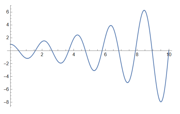
Figure 1: Solution (55) of the fractional harmonic oscillator of order $2.1$ given by (54). For $\mu>2$, the fractional harmonic oscillator mimics an excited oscillator.

Solving (54) using the Wolfram Language 13.3 (Wolfram Research,, 2023) function DSolve we obtain

$$y(t)=E\left(\frac{21}{10},-10t^{21/10}\right).$$ (55)

The solution presented in figure 1 is given in terms of the function MittagLefflerE, the primary function for fractional calculus applications. Its role in FDE solutions is similar in importance to the Exp function for ODE solutions: any FDE with constant coefficients can be solved in terms of Mittag-Leffler functions.

An interesting example is the solution of a fractional harmonic oscillator of order 1.9:

$${}^{\text{C}}_{0}D_{t}^{\frac{19}{10}}x(t)+x(t)=0,\quad x(0)=1,\quad x^{\prime}(0)=0.$$ (56)

Solving (56) using the Wolfram Language 13.3 (Wolfram Research,, 2023) function DSolve we obtain the solution

$$\textbf{fracOsc}:\;x(t)=E\left(\frac{19}{10},-t^{19/10}\right).$$ (57)

This type of oscillator behaves similarly to the ordinary damped harmonic oscillator

$$x^{\prime\prime}(t)+\frac{3}{20}x^{\prime}(t)+x(t)=0,\quad x(0)=1,\quad x^{\prime}(0)=0,$$ (58)

with solution

$$\textbf{dampedOsc}:\;x(t)=\frac{e^{-3t/40}\left(3\sqrt{1591}\sin\left(\frac{\sqrt{1591}t}{40}\right)+1591\cos\left(\frac{\sqrt{1591}t}{40}\right)\right)}{1591}.$$ (59)

This example highlights how the order of an FDE can act as a control parameter to model complex systems.

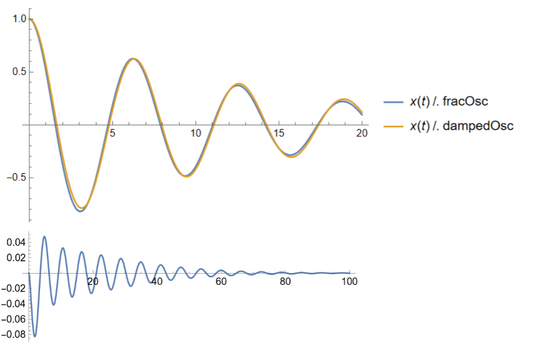
Figure 2: Comparison of the fractional oscillator (57) which satisfies the equation of a fractional harmonic oscillator of order $1.9$ (56) with the damping oscillator (59). The error function is drawn in the bottom plot. That shows that the error between both solutions goes to zero as $t$ becomes large.

Figure 2 shows a comparison of the solution of the fractional oscillator (57) with the damping oscillator (59). The error function is drawn in the bottom plot.

As a final example of FDE, we consider the fractional friction model

$$\ddot{x}(t)+\frac{1}{4}\;{}^{\text{C}}_{0}D_{t}^{\frac{1}{2}}x(t)=0,\quad x(0)=x_{0},\quad x^{\prime}(0)=v_{0}$$ (60)

involving the Caputo fractional differintegral of order $1/2$. Solving (60) using the Wolfram Language 13.3 (Wolfram Research,, 2023) function DSolve we obtain the solution

$$x(t)=x_{0}+tv_{0}E\left(\frac{3}{2},2,-\frac{1}{4}t^{3/2}\right).$$ (61)

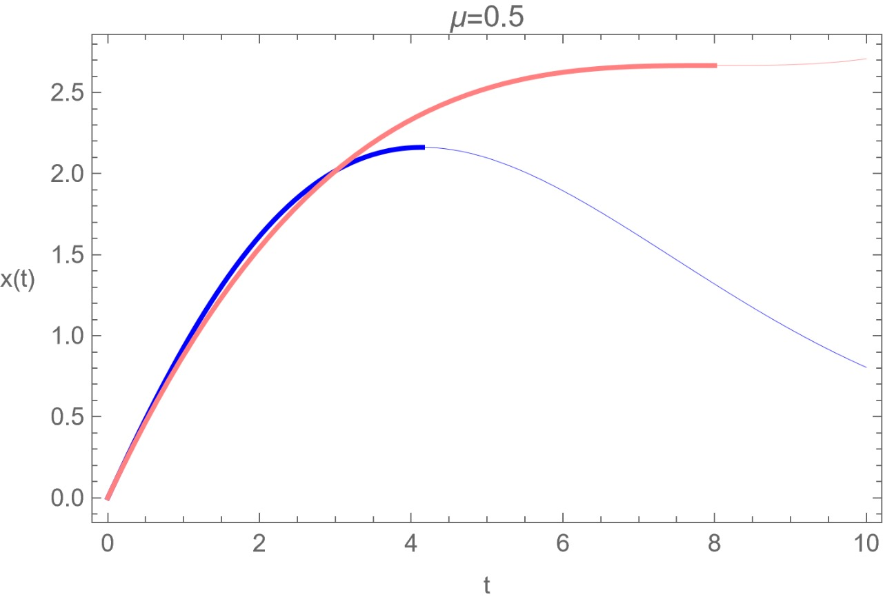
Figure 3: Solution of the FDE (60) for Caputo derivative for $\mu=1/2$, $x_{0}=0$ and $v_{0}=1$ (blue line) and comparison with the solution (100) which gives the position of a point particle under the influence of a velocity-dependent force (pink line).

This solution is given using the functions MittagLefflerE and is represented in figure 3 by a blue line. The pink line corresponds to the solution

$$x(t)=\frac{1}{192}(t-24)t^{2}+t$$ (62)

of the classical Newtonian equation with a friction term

$$\ddot{x}=-\frac{1}{4}\dot{x}^{\frac{1}{2}},\dot{x}>0,$$ (63)

which determines the motion of a point particle influenced by a velocity-dependent force. The thick lines describe the valid motion until the body stops ($v=\dot{x}=0$). The interval is extended to values beyond the physical region (thin lines) for both solutions.

The fractional equivalent of the Newtonian equation of motion, combined with a classical friction term, allows for a broader range of applications than the classical approach. Damped oscillations can be accurately described with a suitable set of fractional initial conditions. From the perspective of fractional calculus, the harmonic oscillator is an example of a fractional friction phenomenon. This implies that friction and damping, described using separate approaches in a classical context, can be combined in the fractional approach. This feature is widespread in the fractional approach and can be applied to various phenomena (Herrmann,, 2014).

II.6 Fractional harmonic oscillator

This section shows the behaviour of fractional derivatives with the property.

$$\lim_{\mu\to 2}D^{\mu}=\frac{d^{2}}{dx^{2}}.$$ (64)

In classical mechanics, the equation that describes free oscillations is

$$\left(\frac{d^{2}}{dt^{2}}+\frac{k}{m}\right)x(t)=0,$$ (65)

whose solution is well known:

$$x(t)=c_{1}\cos{(wt)}+c_{2}\sin{(wt)},\quad w=\sqrt{k/m}.$$ (66)

The fractional formulation of the harmonic oscillator is given by

$$\left(\frac{d^{2\mu}}{dt^{2\mu}}+\frac{k}{m}\right)x(t)=0.$$ (67)

the second-order derivative was directly replaced by one order $2\mu$, where $\mu$ is a fractional number, and the standard harmonic oscillator for $\mu=1$ is recovered.

The solutions of this fractional differential equation for different types of fractional derivatives are presented below, and the specific differences of the solutions obtained are shown.

II.6.1 Fourier harmonic oscillator

When the typical ansatz is proposed for this type of equation (Herrmann,, 2014):

$$x(t)=e^{wt},$$ (68)

the solution to the fractional harmonic oscillator reduces to examining the zeros of the polynomial

$$w^{2\mu}+\frac{k}{m}=0.$$ (69)

In the region $1/2<\mu\leq 3/2$, there are exactly two complex conjugate solutions:

$$w_{1,2}=\left|\frac{k}{m}\right|^{\frac{1}{2\mu}}\left[\cos{\left(\frac{\pi}{2\mu}\right)}\pm i\sin{\left(\frac{\pi}{2\mu}\right)}\right]=\left|\frac{k}{m}\right|^{\frac{1}{2\mu}}e^{\pm i(\frac{\pi}{2\mu})}.$$ (70)

For $\mu=1$, two pure imaginary solutions are obtained, which correspond to a free and undamped oscillation. If $\mu$ begins to decrease, an increasing negative real part occurs, which, from a classical point of view, can be interpreted as increasing damping. For $\mu>1$, we have an increasing positive real part corresponding to increasing excitation (Herrmann,, 2014).

On the other hand, the ordinary differential equation for a damped harmonic oscillator is

$$m\ddot{x}(t)=-kx(t)-\gamma\dot{x}(t),$$ (71)

where $m$ is the mass, $k$ is the spring constant and $\gamma$ is the damping coefficient.

With (68), we have a quadratic equation for the frequency $w$:

$$w^{2}=-\frac{\gamma}{m}w-\frac{k}{m},$$ (72)

Hence, we have two solutions:

$$w_{1,2}=-\frac{\gamma}{2m}\pm\sqrt{\frac{\gamma^{2}}{4m^{2}}-\frac{k}{m}}.$$ (73)

Comparing with (70), we have to

$$-\frac{\gamma}{2m}=\left|\frac{k}{m}\right|^{\frac{1}{2\mu}}\cos{\left(\frac{\pi}{2\mu}\right)},$$ (74)

and with a Taylor series expansion for $\cos{(\pi/2\mu)}$ around $\mu=1$, we have

$$-\frac{\gamma}{2m}\approx\left|\frac{k}{m}\right|^{\frac{1}{2\mu}}\frac{1}{2}\pi(\mu-1).$$ (75)

Near $\mu=1/2$, there is no longer any oscillating contribution. The time evolution of this system is dominated by exponential decay. On the other hand, $\mu>1$ corresponds to a negative classical friction coefficient. Consequently, we have the surprising result that the behaviour of the solutions of the fractional harmonic oscillator under the variation of the fractional derivative parameter, $\mu$, can be interpreted from a classical point of view as damping and excitation phenomena, respectively (Herrmann,, 2014).

The following initial conditions are introduced:

$$x(t=0)=x_{0},$$ (76)

$$D^{\mu}x(t)|_{t=0}=\tilde{v}(t=0)=\tilde{v}_{0}$$ (77)

to compare solutions for different types of fractional derivatives.

Only for $\mu=1$, these initial conditions correspond to the classical initial conditions. For all other cases, the physical interpretation of a fractional velocity remains open.

The solutions of the fractional harmonic oscillator can be reformulated: A first set with the fractional initial conditions $x_{0}=1$, $\tilde{v}_{0}=0$ can be considered as a fractional extension of the standard cosine function, while the fractional initial conditions $x_{0}=0$, $\tilde{v}_{0}=1$ characterize the fractional extension of the sine function:

$${}_{\text{F}}{\sin{(\mu,t)}}=\frac{1}{2i}\left[e^{\frac{1}{2}(e^{\frac{i\pi}{2\mu}})\pi t}-e^{\frac{1}{2}(e^{-\frac{i\pi}{2\mu}})\pi t}\right],$$ (78)

$${}_{\text{F}}{\cos{(\mu,t)}}=\frac{1}{2}\left[e^{\frac{1}{2}(e^{\frac{i\pi}{2\mu}})\pi t}+e^{\frac{1}{2}(e^{-\frac{i\pi}{2\mu}})\pi t}\right].$$ (79)

An appropriately chosen linear combination of these two extended trigonometric functions will again satisfy the classical initial conditions $x(t=0)=x_{0}$ and $v(t=0)=v_{0}$. A graphical representation of these solutions (78) and (79) for different $\mu$ is shown in figure 4.

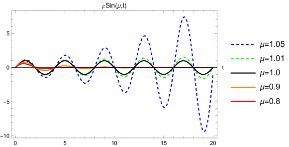
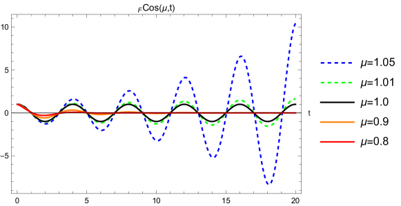
Figure 4: Solutions ${}_{\text{F}}{\sin{(\mu,t)}}$ and ${}_{\text{F}}{\cos{(\mu,t)}}$ of the fractional harmonic oscillator using the Fourier derivative with different values of $\mu$.

II.6.2 Harmonic oscillator according to Riemann

To solve the differential equation of the harmonic oscillator, based on the Riemann fractional derivative, a series expansion is used according to (19). As

$${}_{\text{R}}{D^{\mu}}t^{n\mu}=\frac{\Gamma(1+n\mu)}{\Gamma(1+(n-1)\mu)}t^{(n-1)\mu},$$ (80)

there are two linearly independent solutions, which are called ${}_{\text{R}}{\sin{(\mu,t)}}$ and ${}_{\text{ R}}{\cos{(\mu,t)}}$, in analogy to trigonometric functions:

$${}_{\text{R}}{\sin{(\mu,t)}}=t^{\mu-1}\sum_{n=0}^{\infty}(-1)^{n}\frac{t^{(2n+1)\mu}}{\Gamma((2n+2)\mu)},$$ (81)

$${}_{\text{R}}{\cos{(\mu,t)}}=t^{\mu-1}\sum_{n=0}^{\infty}(-1)^{n}\frac{t^{2n\mu}}{\Gamma((2n+1)\mu)},$$ (82)

with the property

$${}_{\text{R}}D^{\mu}_{\text{R}}{\sin(\mu,wt)}=w^{\mu}_{\text{R}}{\cos{(\mu,wt)}},$$ (83)

$${}_{\text{R}}D^{\mu}_{\text{R}}{\cos(\mu,wt)}=-w^{\mu}_{\text{R}}{\sin{(\mu,wt)}}.$$ (84)

These functions are related to the Mittag-Leffler function (272):

$${}_{\text{R}}{\sin{(\mu,t)}}=t^{2\mu-1}E(2\mu,2\mu,-t^{2\mu}),$$ (85)

$${}_{\text{R}}{\cos{(\mu,t)}}=t^{\mu-1}E(2\mu,\mu,-t^{2\mu}).$$ (86)

For $\mu<1$, it holds that

$$\lim_{t\to 0}{}_{\text{R}}{\cos{(\mu,wt)}}=\infty,$$ (87)

which means that a non-singular solution that satisfies the general initial conditions (76) cannot be given. At first glance, this seems to be a serious drawback for practically applying the fractional Riemann derivative. Nevertheless, it must be considered that the solutions presented can be useful for problems not determined by the initial conditions but are formulated in terms of boundary conditions, as is the case, for example, of the solutions of a wave equation (Herrmann,, 2014).

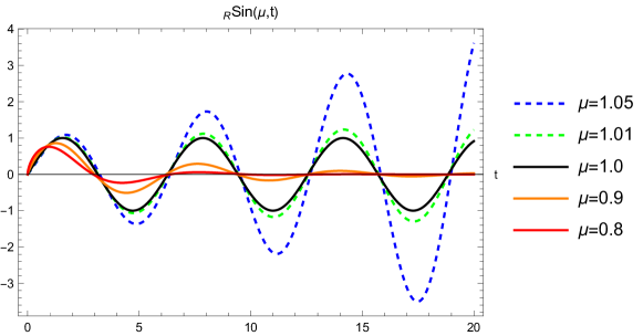
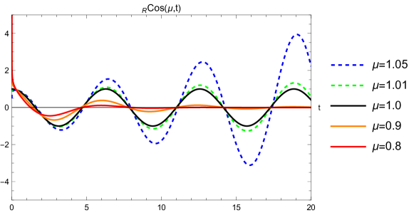
Figure 5: Solutions ${}_{\text{R}}{\sin{(\mu,t)}}$ and ${}_{\text{R}}{\cos{(\mu,t)}}$ of the fractional harmonic oscillator using the Riemann derivative for different values of $\mu$.

Solutions ${}_{\text{R}}{\sin{(\mu,t)}}$ and ${}_{\text{R}}{\cos{(\mu,t)}}$ of the fractional harmonic oscillator using the Riemann derivative are presented in figure 5 for different values of $\mu$.

II.6.3 Harmonic oscillator according to Caputo

This solution can be written as a series according to (21). The Caputo derivative for a power is given by

$${}^{\text{C}}{D^{\mu}}t^{n\mu}=\left\{\begin{array}[]{lcc}\frac{\Gamma(1+n\mu)}{\Gamma(1+(n-1)\mu)}t^{(n-1)\mu},&n>0,\\ \\ 0,&n=0.\end{array}\right.$$ (88)

Therefore, we have two linearly independent solutions, which are called ${}_{\text{C}}{\sin{(\mu,t)}}$ and ${}_{\text{C}}{\cos{(\mu,t)}}$, in analogy to trigonometric functions:

$${}_{\text{C}}{\sin{(\mu,t)}}=\sum_{n=0}^{\infty}(-1)^{n}\frac{t^{(2n+1)\mu}}{\Gamma(1+(2n+1)\mu)},$$ (89)

$${}_{\text{C}}{\cos{(\mu,t)}}=\sum_{n=0}^{\infty}(-1)^{n}\frac{t^{2n\mu}}{\Gamma(1+2n\mu)}.$$ (90)

The most important property of this series is:

$${}^{\text{C}}{D^{\mu}}{}_{\text{C}}{\sin{(\mu,wt)}}=w^{\mu}{}_{\text{C}}{\cos{(\mu,wt)}},$$ (91)

$${}^{\text{C}}{D^{\mu}}{}_{\text{C}}{\cos{(\mu,wt)}}=-w^{\mu}{}_{\text{C}}{\sin{(\mu,wt)}}.$$ (92)

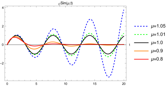
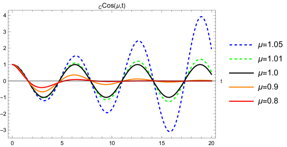
Figure 6: Solutions ${}_{\text{C}}{\sin{(\mu,t)}}$ and ${}_{\text{C}}{\cos{(\mu,t)}}$ of the fractional harmonic oscillator using the Caputo derivative for different values of $\mu$.

Solutions ${}_{\text{C}}{\sin{(\mu,t)}}$ and ${}_{\text{C}}{\cos{(\mu,t)}}$ of the fractional harmonic oscillator using the Caputo derivative are presented in figure 6 for different values of $\mu$.

After comparing the solutions obtained from different definitions of the fractional derivative for the differential equation of the harmonic oscillator, we notice a remarkable similarity among the presented solutions. They all display oscillatory behaviour with exponential decay when $\mu<1$, which can be interpreted as a classical damping phenomenon. On the other hand, for $\mu>1$, the fractional harmonic oscillator acts as an excited oscillator. The damping and excitation properties are inherent to the fractional oscillator and do not stem from external factors. In a study by Stanislavsky (Stanislavsky,, 2004), a multiparticle statistical interpretation was proposed as a physical explanation of the fractional harmonic oscillator.

Moreover, the frequency of these damped oscillations is quite similar for the various definitions of fractional derivatives presented, especially for a value of $\mu$ approximating 1. Therefore, it can be regarded as an independent property of the definition (Herrmann,, 2014).

II.7 Fractional Friction

The evolution of the position $x(t)$ and the velocity $v(t)=\dot{x}(t)=\frac{d}{dt}x(t)$ of a point particle as functions of time caused by an external force $F$ is determined by Newton’s second law

$$F=ma=m\ddot{x}(t)=m\frac{d^{2}}{dt^{2}}x(t).$$ (93)

In the absence of external forces, the solution continues to integrate twice $\ddot{x}=0$:

$$x(t)=x_{0}+v_{0}t,$$ (94)

where the constants of integration are the position $x(0)=x_{0}$ and initial velocity $v(0)=v_{0}$ and $\dot{x}(t)=v_{0}$ for all $t$. That means the point mass maintains its initial velocity forever without external forces. That is what is known as Newton’s first law. However, daily experience of movement contradicts this result. Sooner or later, without external intervention, all types of movement end at rest. Within the framework of Newtonian theory, all these observed phenomena are due to friction forces $F_{R}$.

All friction forces point in the opposite direction to the particle’s speed. Empirically, a power law function can be proposed:

$$F_{R}=-\alpha\text{sgn}(v)|v|^{\mu},$$ (95)

where $\mu$ is an arbitrary real exponent. Some special cases are $\mu\approx 0$, which is observed for static and kinetic pressure in solids, while $\mu=1$ corresponds to the Stokes friction of a liquid with high viscosity and $\mu=2$, which is a general trend towards high speed (Herrmann,, 2014).

Let us consider the differential equation

$$m\ddot{x}=-\alpha\text{sgn}(v)|v|^{\mu},$$ (96)

where the mass $m$ is measured in kilogram $[kg]$ and the friction coefficient $\alpha$ is measured in $kg/s^{2-\mu}$, which describes the dynamics of a point particle under the effect of a friction force of the type (95).

Assuming that the velocity is positive, we have

$$m\ddot{x}=-\alpha\dot{x}^{\mu},\dot{x}>0.$$ (97)

Imposing the initial conditions

$$x(t=0)=x_{0},$$ (98)

$$v(t=0)=v_{0},$$ (99)

we obtain the general solution of (97) given by

$$x(t)=x_{0}+\frac{mv_{0}^{2-\mu}}{\alpha(2-\mu)}-\frac{m\left[(\mu-1)(-\frac{v_{0}^{1-\mu}}{1-\mu}+\frac{\alpha}{m}t)\right]^{\frac{2-\mu}{1-\mu}}}{\alpha(2-\mu)}.$$ (100)

The equation (100) determines the motion of a point particle under the influence of a velocity-dependent force for an arbitrary $\mu$.

The special cases $\mu=0$, $\mu=1$ and $\mu=2$ are included as special limits (Herrmann,, 2014)

$$\lim_{\mu\rightarrow 0}x(t)=x_{0}+v_{0}t-\frac{1}{2}\frac{\alpha}{m}t^{2},$$ (101)

$$\lim_{\mu\rightarrow 1}x(t)=x_{0}+\frac{m}{\alpha}v_{0}\left(1-e^{-\frac{\alpha}{m}t}\right),$$ (102)

$$\lim_{\mu\rightarrow 2}x(t)=x_{0}+\frac{m}{\alpha}\ln\left(1+\frac{\alpha}{m}v_{0}t\right).$$ (103)

Finally, the modification of Newton’s equation (97) is studied according to (Herrmann,, 2014) where the friction force $F_{R}(\dot{x})=-\alpha\dot{x}(t)^{\mu}$ has been replaced by the fractional friction force:

$$F_{R}=-\alpha D_{t}^{\mu}x(t),\hskip 20.075pt\dot{x}(t)>0,$$ (104)

where $\mu$ is the order of the fractional derivative. For $\mu\neq 1$ and $t>0$, we have to

$$\dot{x}^{\mu}=\left(\frac{d}{dt}x(t)\right)^{\mu}\neq D_{t}^{\mu}x(t),$$ (105)

so it is expected that the solutions of the fractional equation

$$m\ddot{x}(t)+\alpha D_{t}^{\mu}x(t)=0$$ (106)

have behaviour different from the standard. Note that to compare with the classical damped harmonic oscillator given by (71), we have renamed the friction constant $\alpha$.

Replacing the ansatz $x(t)=e^{wt}$ into (106), and applying Liouville’s definition, we have:

$$D_{t}^{\mu}e^{wt}=w^{\mu}e^{wt}.$$ (107)

Therefore, the characteristic polynomial of (106) is

$$w^{2}=-\frac{\alpha}{m}w^{\mu}.$$ (108)

In addition to the trivial solution, we have the solution

$$w=(-1)^{\frac{1}{2-\mu}}\left|\frac{\alpha}{m}\right|^{\frac{1}{2-\mu}}.$$ (109)

For $0<\mu<1$, and using the abbreviation

$$\kappa=\left|\frac{\alpha}{m}\right|^{\frac{1}{2-\mu}},$$ (110)

There are two complex conjugate solutions:

$$w_{1,2}=\kappa\left[\cos{\left(\frac{\pi}{2-\mu}\right)\pm i\sin{\left(\frac{\pi}{2-\mu}\right)}}\right].$$ (111)

So the general solution of (106) is

$$x(t)=c_{1}+c_{2}e^{w_{1}t}+c_{3}e^{w_{2}t},\hskip 20.075pt0<\mu<1.$$ (112)

It is observed that there are three different constants $c_{i}$, two of which can be determined using the initial conditions $x(t=0)=x_{0}$ and $v(t=0):=\dot{x}(0)=v_{0}$. Consequently, the freedom to specify an additional reasonable initial condition indicates that the fractional differential equation (106) describes a broader range of phenomena than the classical equation (Herrmann,, 2014).

Starting from (106), the condition can be considered

$$\ddot{x}(t=0)=-\frac{\alpha}{m}v_{0}^{\mu}.$$ (113)

Therefore, the set of equations is obtained

$$\begin{pmatrix}1&1&1\\ 0&w_{1}&w_{2}\\ 0&w_{1}^{2}&w_{2}^{2}\end{pmatrix}\begin{pmatrix}c_{1}\\ c_{2}\\ c_{3}\end{pmatrix}=\begin{pmatrix}x_{0}\\ v_{0}\\ -\frac{\alpha}{\mu}v_{0}^{\mu}\end{pmatrix}.$$ (114)

Then, the solution of the fractional differential equation (106) is

$$x(t)\approx x_{0}+v_{0}t-\frac{1}{2}\frac{\alpha}{\mu}v_{0}^{\mu}t^{2}-\frac{t^{3}\left(2\alpha\cos\left(\frac{\pi}{\mu-2}\right)v_{0}^{\mu}\left|\frac{\alpha}{m}\right|^{\frac{1}{2-\mu}}+mv_{0}\left|\frac{m}{\alpha}\right|^{\frac{2}{\mu-2}}\right)}{6m}+o(t^{4}).$$ (115)

If the condition is chosen

$$\ddot{x}(t=0)=0,$$ (116)

the set of equations is obtained

$$\begin{pmatrix}1&1&1\\ 0&w_{1}&w_{2}\\ 0&w_{1}^{2}&w_{2}^{2}\end{pmatrix}\begin{pmatrix}c_{1}\\ c_{2}\\ c_{3}\end{pmatrix}=\begin{pmatrix}x_{0}\\ v_{0}\\ 0\end{pmatrix},$$ (117)

and in this case, the complete solution is

$$x(t)=x_{0}+\frac{v_{0}}{\kappa\sin{\left(\frac{\pi}{2-\mu}\right)}}\left[e^{\kappa\cos{\left(\frac{\pi}{2-\mu}\right)}t}\sin{\left(\frac{2\pi}{2-\mu}-\kappa\sin{\left(\frac{\pi}{2-\mu}\right)}t\right)}-\sin{\left(\frac{2\pi}{2-\mu}\right)}\right],$$ (118)

which is valid from $t=0$ until a final time $t_{f}$ in which the mass comes to rest, which is determined by the equation

$$t_{f}=\frac{\pi}{(2-\mu)\kappa\sin{\left(\frac{\pi}{2-\mu}\right)}}.$$ (119)

Let us compare the classical damped harmonic oscillator given by (71). The two solutions of the classical damped harmonic oscillator are:

$$w_{1,2}=-\frac{\gamma}{2m}\pm\sqrt{\frac{\gamma^{2}}{4m^{2}}-\frac{k}{m}},$$ (120)

where $\gamma$ is the damping coefficient in (71). By comparing the $w_{i}$ of (111) and (120), the relations are obtained

$$\frac{k}{m}=\left(\frac{\alpha}{\mu}\right)^{\frac{2}{2-\mu}}$$ (121)

and

$$\frac{\gamma}{m}=-2\left(\frac{\alpha}{\mu}\right)^{\frac{1}{2-\mu}}\cos{\left(\frac{\pi}{2-\mu}\right)}.$$ (122)

These relations describe the behaviour of the solutions of the fractional friction differential equation as investigated in (Herrmann,, 2014).

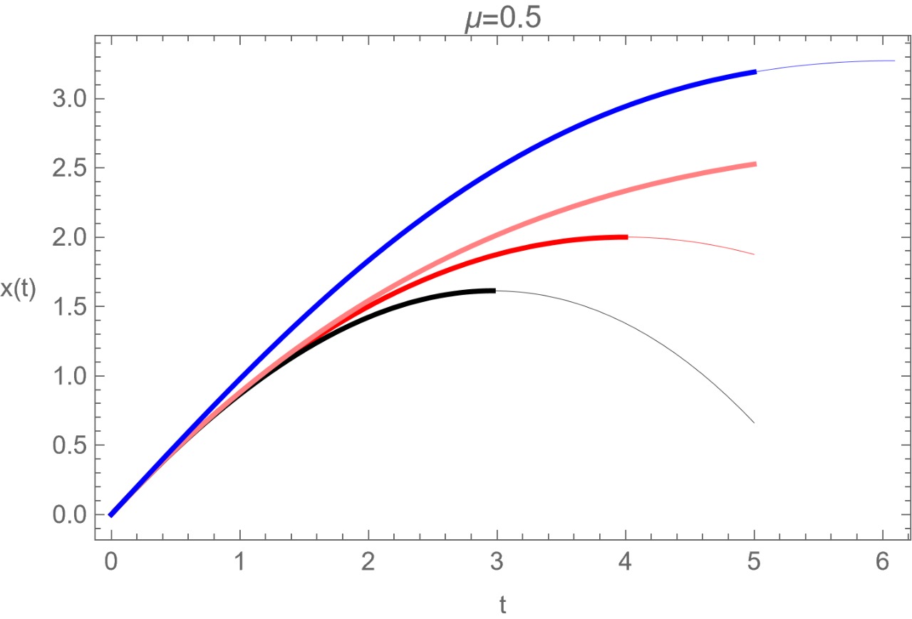
Figure 7: Different solutions of the equation of motion (106) with $\mu=0.5$, $x_{0}=0$, $v_{0}=1$, $m=1$, $\alpha=0.25$ (Herrmann,, 2014).

In the figure 7, different solutions of the fractional friction equation (106) and the solution of the classical equation (pink) $m\ddot{x}=-\alpha\dot{x}^{\mu}$ given by (100) are presented. In red (up to order 2) and black (up to order 3), the solutions to the fractional friction equation (106) given by the equation (115) are presented. The blue line represents the solution (118) with initial condition $\ddot{x}(0)=0$ (Herrmann,, 2014).

It is observed that the classical solution and the corresponding fractional solution with the initial condition (113) coincide up to the second order in $t$, and there is a difference only at the end of the movement. The thick lines describe the valid motion until the body stops ($v=\dot{x}=0$). Furthermore, for both fractional solutions, the plot interval is extended to values $t>t_{f}$ (thin lines) beyond the physical region.

When the fractional parameter $\mu$ approaches zero, the behaviour approaches that of damping. Near $\mu=2$, fractional friction acts as an acceleration term, and for the ideal case, $\mu=2$, the differential equation for a free particle is recovered.

Using fractional calculus, we can expand beyond the classical approach by combining the fractional equivalent of the Newtonian equation of motion with a classical friction term. This allows us to describe a wider range of phenomena, including damped oscillations with fractional initial conditions. The harmonic oscillator is an example of a fractional friction phenomenon, where friction and damping can be unified.

It is important to note that the fractional differential equation represented by (106) combines two different types of classical differential equations. Nonlinear differential equations generally have complex solutions, whereas a simple second-order differential equation with constant coefficients can be solved using the same fractional equation. This observation suggests that a wide range of complex problems can be solved analytically using fractional calculus with minimal effort. On the other hand, a solution obtained from a classical theory may be more complicated.

In this section, we build upon previous research in the field (Herrmann,, 2014) and emphasize the importance of fractional calculus in explaining physical phenomena. We then explore the applications of this concept in theories of gravity to provide a better understanding of the complex mathematical structure of the universe. The next section aims to use advanced mathematical techniques to create new formulations and tools which will help us better comprehend the cosmos. This is a crucial aspect of our research.

III Gravity models with fractional derivatives

In the last section, we discussed the importance of fractional calculus in understanding physical phenomena. Now, we will focus on its applications to theories of gravity for a better understanding of the universe’s mathematical structure.

The Lagrangian density is a mathematical tool used to model the dynamic properties of fields (Baleanu and Muslih,, 2005; Agrawal,, 2007; El-Nabulsi and Torres,, 2008; Baleanu and Trujillo,, 2010; Odzijewicz et al., 2013a, ; Odzijewicz et al., 2013b, ; Odzijewicz et al., 2013c, ). Fractional Lagrangian densities have gained popularity in addressing cosmological problems. Fractional calculus defines Riemann curvature and the Einstein tensor, dependent on the fractional parameter $\mu$. The fractional Einstein tensor equation, $G_{\alpha\beta}(\mu)=8\pi GT_{\alpha\beta}(\mu)$, where $G_{\alpha\beta}(\mu)$ is the fractional Einstein tensor, has been modified to study various cosmological events. For example, a fractional theory of gravitation has been developed for fractional spacetime, leading to new classes of cosmological models. These models have been studied in great detail  (Vacaru,, 2010; Vacaru, 2012a, ; Vacaru, 2012b, ; Jamil et al.,, 2012; El-Nabulsi,, 2012; El-Nabulsi, 2013a, ; El-Nabulsi, 2013b, ; El-Nabulsi, 2013c, ; El-Nabulsi, 2016a, ; El-Nabulsi, 2016b, ; El-Nabulsi, 2017a, ; El-Nabulsi, 2017c, ; Debnath et al.,, 2012, 2013; Roberts,, 2014; Shchigolev,, 2011; Shchigolev, 2013a, ; Shchigolev, 2013b, ; Shchigolev,, 2016, 2021; Rami,, 2015; Calcagni,, 2013; Calcagni, 2017a, ; Calcagni, 2017b, ; Calcagni, 2021a, ; Calcagni, 2021b, ; Calcagni, 2021c, ; Calcagni et al.,, 2016, 2019; Calcagni and Kuroyanagi,, 2021; Calcagni and De Felice,, 2020; Giusti,, 2020; Jalalzadeh et al.,, 2022; Landim, 2021a, ; Landim, 2021b, ; García-Aspeitia et al.,, 2022; Micolta-Riascos et al.,, 2023). In reference (García-Aspeitia et al.,, 2022), a joint analysis was performed using cosmic chronometers and type Ia supernovae data. This comparison with observational tests was used to find the best-fit values for the fractional order of the derivative. These methods are a robust scheme to investigate the physical behaviour of cosmological models (Hernández-Almada et al.,, 2020; Leon et al.,, 2021; Hernández-Almada et al.,, 2021, 2022; García-Aspeitia et al.,, 2022). They can be used in new contexts, such as  (Micolta-Riascos et al.,, 2023), where dynamical systems were used to analyze a fractional cosmology for different matter contents, obtaining a cosmology with late acceleration without including dark energy. References (García-Aspeitia et al.,, 2022; González et al.,, 2023; Leon Torres et al.,, 2023) have explored the potential of fractional cosmology to address the $H_{0}$ tension (Di Valentino et al.,, 2021; Efstathiou,, 2021) from the Supernova data and the Planck value for $z<1.5$ and have reported a trend of $H_{0}$ that aligns with these values. However, a discrepancy exists between the $1.5<z<2.5$ range values, indicating that the tension $H_{0}$ has not been entirely resolved.

Based on the work presented in (García-Aspeitia et al.,, 2022), two research paths were identified for the cosmological model without a scalar field. The first path involves comparing it with the standard model, imposing that the components of the Universe are cold dark matter and radiation. The second path consists of deducing the equation of state for one of the sources of matter from compatibility conditions (Micolta-Riascos et al.,, 2023), which had not been previously analyzed in (García-Aspeitia et al.,, 2022).

III.1 Cosmological model in the fractional formulation of gravity

There are two established methods for incorporating fractional derivatives into cosmology under the classical regime. The simplest method is the modification method, which replaces the cosmological field equations of a given model with corresponding fractional field equations. An example of this can be found in Barrientos et al., (2021). The more fundamental methodology is the first-step modification method. This method involves defining the fractional derivative and establishing the variational principle of fractional action (El-Nabulsi,, 2005; El-Nabulsi, 2007a, ; El-Nabulsi, 2007b, ; El-Nabulsi,, 2008; Frederico and Torres,, 2008; Roberts,, 2014) to obtain a modified cosmological model. Given the fractional integral action,

$$S(\tau) =\frac{1}{\Gamma(\mu)}\int_{0}^{\tau}\mathcal{L}\left(\theta,q_{i}(\theta),\dot{q}_{i}(\theta),\ddot{q}_{i}(\theta)\right)(\tau-\theta)^{\mu-1}d\theta,$$ (123)

where $\Gamma(\mu)$ is the Gamma function, $\mathcal{L}$ the Lagrangian, $\mu$ the constant fractional parameter, $\tau$ and $\theta$ are the physical and intrinsic time respectively.

Varying the action (123) with respect to $q_{i}$ we obtain the Euler-Poisson equations (Frederico and Torres,, 2008),

$$\frac{\partial\mathcal{L}\left(\theta,q_{i}(\theta),\dot{q}_{i}(\theta),\ddot{q}_{i}(\theta)\right)}{\partial q_{i}}-\frac{d}{d\theta}\frac{\partial\mathcal{L}\left(\theta,q_{i}(\theta),\dot{q}_{i}(\theta),\ddot{q}_{i}(\theta)\right)}{\partial\dot{q}_{i}}+\frac{d^{2}}{d\theta^{2}}\frac{\partial\mathcal{L}\left(\theta,q_{i}(\theta),\dot{q}_{i}(\theta),\ddot{q}_{i}(\theta)\right)}{\partial\ddot{q}_{i}}$$

$$=\frac{1-\mu}{\tau-\theta}\left(\frac{\partial\mathcal{L}\left(\theta,q_{i}(\theta),\dot{q}_{i}(\theta),\ddot{q}_{i}(\theta)\right)}{\partial\dot{q}_{i}}-2\frac{d}{d\theta}\frac{\partial\mathcal{L}\left(\theta,q_{i}(\theta),\dot{q}_{i}(\theta),\ddot{q}_{i}(\theta)\right)}{\partial\ddot{q}_{i}}\right)$$

$$-\frac{\left(1-\mu\right)\left(2-\mu\right)}{\left(\tau-\theta\right)^{2}}\frac{\partial\mathcal{L}\left(\theta,q_{i}(\theta),\dot{q}_{i}(\theta),\ddot{q}_{i}(\theta)\right)}{\partial\ddot{q}_{i}}.$$ (124)

In cosmology it is assumed that the flat Friedmann–Lemaître–Robertson–Walker (FLRW) metric

$$ds^{2}=-N^{2}(t)dt^{2}+a^{2}(t)(dx^{2}+dy^{2}+dz^{2}),$$ (125)

is the spacetime metric, where $a(t)$ denotes the scale factor and $N(t)$ is the lapse function. This result is supported observationally with data from the Planck’s (Aghanim et al.,, 2020) probe. For the metric (125), the  Ricci scalar depends on up to second derivatives of $a$ and first derivatives of $N$, which is written as

$$R(t)=6\Bigg{(}\frac{\ddot{a}(t)}{a(t)N^{2}(t)}+\frac{{\dot{a}}^{2}(t)}{a^{2}(t)N^{2}(t)}-\frac{\dot{a}(t)\dot{N}(t)}{a(t)N^{3}(t)}\Bigg{)}.$$ (126)

Thus, we can consider the integral action in units where $8\pi G=c=1$:

$$S(\tau) =\int_{0}^{\tau}\left[\frac{R(\theta)}{2}+\frac{\dot{\phi}^{2}(\theta)}{2N^{2}(\theta)}-V(\phi(\theta))+\xi R(\theta)\phi^{2}(\theta)+{L}_{\text{matter}}(\theta)\right]a^{3}(\theta)N(\theta)d\theta,$$ (127)

where $R(\theta)$ is the Ricci scalar (126). In cosmology, the Einstein-Hilbert Lagrangian density is related to the Ricci scalar. Generically, integration by parts is taken so that a total derivative in the action is eliminated, as well as the derivatives $\ddot{a}(t)$ and $\dot{N}(t)$. However, since we will use a fractional version of the Lagrangian (127), we will not follow the standard procedure and will keep the higher-order derivatives. Using the formulation (123), the Euler-Poisson equation (124) is obtained, which involves fractional variational calculus with classical and Caputo derivatives. If ${L}_{\text{matter}}(\theta)=-\rho_{0}a(\theta)^{-3(1+w)}$ for $w\neq-1$, we recover the usual Lagrangian density of matter of a perfect fluid as in  (Wald,, 2010; Carroll,, 2019; Carroll et al.,, 2004) containing derivatives of integer order in the Lagrangian. To extend the theory given by the effective fractional action used in (García-Aspeitia et al.,, 2022), we can assume the Einstein-Hilbert action and add a scalar field $\phi$ to create a scalar field theory with coupling $\xi R\phi^{2}$ between gravity and the scalar field, with $\xi$ being the coupling constant. The simplest and most natural case is the minimal coupling where $\xi=0$. Another viable option is $\xi=1/6$, known as conformal coupling because the action does not change under conformal transformations of the metric. Any value of the coupling parameter $\xi\neq 0$ is a non-minimal coupling.

The resulting action is

$$S_{{\text{eff}}}(\tau) =\frac{1}{\Gamma(\mu)}\int_{0}^{\tau}\mathcal{L}\left(\theta,N(\theta),\dot{N}(\theta),a(\theta),\dot{a}(\theta),\ddot{a}(\theta),\phi(\theta),\dot{\phi}(\theta)\right)(\tau-\theta)^{\mu-1}d\theta,$$ (128)

where $\Gamma(\mu)$ is the Gamma function, and the Lagrangian density is

$$\mathcal{L}\left(\theta,N(\theta),\dot{N}(\theta),a(\theta),\dot{a}(\theta),\ddot{a}(\theta)\right) :=\frac{3a(\theta)\left(N(\theta)\left(a(\theta)\ddot{a}(\theta)+\dot{a}^{2}(\theta)\right)-a(\theta)\dot{a}(\theta)\dot{N}(\theta)\right)}{N^{2}(\theta)}$$

$$+a^{3}(\theta)N(\theta)\left(\frac{\dot{\phi}^{2}(\theta)}{2N^{2}(\theta)}-V(\phi(\theta))\right)$$

$$-\rho_{0}N(\theta)a(\theta)^{-3w}(\tau-\theta)^{-(\mu-1)(w+1)}$$

$$-\frac{3\xi\phi^{2}(\theta)a(\theta)\left(N(\theta)\left(a(\theta)\ddot{a}(\theta)+\dot{a}^{2}(\theta)\right)-a(\theta)\dot{a}(\theta)\dot{N}(\theta)\right)}{N^{2}(\theta)},$$ (129)

$w=p/\rho$ is a constant state equation parameter for matter, $\phi$ is the scalar field, and $V$ is its interaction potential, depending on the scalar field.

The Euler–Poisson equations (124) are derived after varying the action (128) with respect to $q_{i}\in\{N,a,\phi\}$, obtaining the equations

$$\left(1-\xi\phi^{2}(\theta)\right)\left[\left(\frac{\dot{a}(\theta)}{a(\theta)}\right)^{2}+\left(\frac{\dot{a}(\theta)}{a(\theta)}\right)\left(\frac{1-\mu}{\tau-\theta}\right)\right]$$

$$=\frac{1}{3}\rho_{m0}a(\theta)^{-3w-3}(\tau-\theta)^{-(\mu-1)(w+1)}+\frac{1}{6}\left(\dot{\phi}^{2}(\theta)+2V(\phi(\theta))\right)+2\xi\frac{\dot{a}(\theta)\phi(\theta)\dot{\phi}(\theta)}{a(\theta)},$$ (130)

$$\left(1-\xi\phi^{2}(\theta)\right)\left[\frac{\ddot{a}(\theta)}{a(\theta)}+\frac{1}{2}\left(\frac{\dot{a}(\theta)}{a(\theta)}\right)^{2}+\frac{(1-\mu)}{(t-\theta)}\frac{\dot{a}(\theta)}{a(\theta)}+\frac{(\mu-2)(\mu-1)}{2(\tau-\theta)^{2}}\right]$$

$$=-\frac{1}{2}\rho_{0}wa(\theta)^{-3(1+w)}(\tau-\theta)^{-(\mu-1)(w+1)}-\frac{1}{4}\dot{\phi}^{2}(\theta)+\frac{1}{2}V(\phi(\theta))$$

$$+\xi\left[\frac{2\phi(\theta)\dot{a}(\theta)\dot{\phi}(\theta)}{a(\theta)}+\frac{2(1-\mu)\phi(\theta)\dot{\phi}(\theta)}{\tau-\theta}+\phi(\theta)\ddot{\phi}(\theta)+\dot{\phi}^{2}(\theta)\right],$$ (131)

$$\ddot{\phi}(\theta)+\frac{3\dot{a}(\theta)\dot{\phi}(\theta)}{a(\theta)}+\frac{(1-\mu)\dot{\phi}(\theta)}{\tau-\theta}+V^{\prime}(\phi(\theta))=-6\xi\phi(\theta)\left[\frac{\ddot{a}(\theta)}{a(\theta)}+\left(\frac{\dot{a}(\theta)}{a(\theta)}\right)^{2}\right],$$ (132)

and the conservation of matter equation

$$\dot{\rho}(\theta)=-3\left(\frac{\dot{a}(\theta)}{a(\theta)}+\frac{1-\mu}{3(\tau-\theta)}\right)(\rho(\theta)+p(\theta)),$$ (133)

where we have replaced $N=1$ after the variation of the action (128).

For fixed $\tau$, the expressions

$$\rho(\theta)=\rho_{0}a(\theta)^{-3(1+w)}(\tau-\theta)^{-(\mu-1)(w+1)},$$ (134)

and

$$p(\theta)=w\rho_{0}a(\theta)^{-3(1+w)}(\tau-\theta)^{-(\mu-1)(w+1)},$$ (135)

which define the energy density and isotropic pressure of matter fields.

To designate the temporal independent variables, the rule $(\tau,\theta)\mapsto(2t,t)$ is applied, where the new cosmological time $t$ (Shchigolev,, 2011) is used. Hereafter, dots mean derivative with respect to $t$.

Furthermore, the parameter  Hubble is $H\equiv\dot{a}/a$. Therefore, the equations (130) and (131), the modified Klein-Gordon equation (132), and the conservation equation (133) can be written as

$$\left(1-\xi\phi^{2}(t)\right)\left(\dot{H}(t)+\frac{(1-\mu)H(t)}{t}+\frac{3H^{2}(t)}{2}+\frac{(\mu-2)(\mu-1)}{2t^{2}}\right)$$

$$=-\frac{1}{2}p(t)-\frac{1}{4}\dot{\phi}(t)^{2}+\frac{1}{2}V(\phi(t))+\xi\phi(t)\left(2H(t)\dot{\phi}(t)-\frac{2(\mu-1)\dot{\phi}(t)}{t}+\ddot{\phi}(t)+\dot{\phi}(t)\right),$$ (136)

$$\left(1-\xi\phi^{2}(t)\right)\left(H^{2}(t)+\frac{(1-\mu)H(t)}{t}\right)=\frac{1}{3}\rho(t)+\frac{1}{6}\dot{\phi}^{2}(t)+\frac{1}{3}V(\phi(t))+2\xi H(t)\phi(t)\dot{\phi}(t),$$ (137)

$$\ddot{\phi}(t)+3H(t)\dot{\phi}(t)-\frac{(\mu-1)\dot{\phi}(t)}{t}+V^{\prime}(\phi(t))=-\xi\phi(t)\left(6\dot{H}(t)+12H(t)^{2}\right),$$ (138)

$$\dot{\rho}(t)=-3\left(H(t)+\frac{(1-\mu)}{3t}\right)(p(t)+\rho(t)).$$ (139)

We observe that the equation (139) is satisfied for any value of the equation of state of matter parameter. Furthermore, by eliminating the higher order derivatives, we obtain the equation (139) and

$$\dot{H} =H\left(\frac{(1-\mu)\left(\xi\phi^{2}-1\right)}{\xi(6\xi-1)t\phi^{2}+t}-\frac{\xi\phi\dot{\phi}}{\xi(6\xi-1)\phi^{2}+1}\right)+\frac{H^{2}\left(3(1-8\xi)\xi\phi^{2}-3\right)}{2\xi(6\xi-1)\phi^{2}+2}-\frac{p}{2\xi(6\xi-1)\phi^{2}+2}$$

$$+\frac{(\mu-2)(\mu-1)\left(\xi\phi^{2}-1\right)}{2t^{2}\left(\xi(6\xi-1)\phi^{2}+1\right)}+\frac{\dot{\phi}\left((4\xi-1)t\dot{\phi}-4(\mu-1)\xi\phi\right)}{4\left(\xi(6\xi-1)t\phi^{2}+t\right)}$$

$$-\frac{\xi\phi V^{\prime}(\phi)}{\xi(6\xi-1)\phi^{2}+1}+\frac{V(\phi)}{2\xi(6\xi-1)\phi^{2}(t)+2},$$ (140)

$$\ddot{\phi} =H\left(\frac{6(\mu-1)\xi\phi\left(\xi\phi^{2}-1\right)}{\xi(6\xi-1)t\phi^{2}+t}-\frac{3\left(\xi(4\xi-1)\phi^{2}+1\right)\dot{\phi}}{\xi(6\xi-1)\phi^{2}+1}\right)$$

$$+\frac{3\xi H^{2}\phi\left(\xi\phi^{2}-1\right)}{\xi(6\xi-1)\phi^{2}+1}+\frac{3\xi p\phi}{\xi(6\xi-1)\phi^{2}+1}-\frac{3(\mu-2)(\mu-1)\xi\phi\left(\xi\phi^{2}-1\right)}{t^{2}\left(\xi(6\xi-1)\phi^{2}+1\right)}$$

$$+\frac{\dot{\phi}\left(2(\mu-1)+\xi\phi\left(2(\mu-1)(12\xi-1)\phi+3(1-4\xi)t\dot{\phi}\right)\right)}{2\left(\xi(6\xi-1)t\phi^{2}+t\right)}$$

$$+\frac{\left(\xi\phi^{2}-1\right)V^{\prime}(\phi)}{\xi(6\xi-1)\phi^{2}+1}-\frac{3\xi\phi V(\phi)}{\xi(6\xi-1)\phi^{2}+1}.$$ (141)

Solving (137) for $\rho$ we obtain

$$\rho=\frac{3H(-tH+\mu-1)\left(\xi\phi^{2}-1\right)}{t}-6\xi H\phi\dot{\phi}-V(\phi)-\frac{1}{2}\dot{\phi}^{2}.$$ (142)

In (Micolta-Riascos et al.,, 2023) the equations (136)–(139) for $\xi=0$ were studied. Using a procedure similar to that of RG, (137) is required to be conserved over time, i.e.

$$\frac{d}{dt}\left[\left(1-\xi\phi^{2}\right)\left(H^{2}+\frac{(1-\mu)H}{t}\right)-\frac{1}{3}\rho-\frac{1}{6}\dot{\phi}^{2}-\frac{1}{3}V(\phi)-2\xi H\phi\dot{\phi}\right]=0.$$ (143)

Calculating the corresponding derivatives and substituting (139), (140), (141) and (142), we obtain

$$\frac{(\mu-1)}{12t^{3}\left(\xi(6\xi-1)\phi^{2}+1\right)}\Bigg{[}-6t^{2}H^{2}\left(\xi\phi^{2}-1\right)^{2}$$

$$+\left(\xi\phi^{2}-1\right)\Big{(}-12tH\left(-\mu+\xi\phi\left((\mu+12\xi-3)\phi+t\dot{\phi}\right)+3\right)$$

$$-12\xi t^{2}\phi V^{\prime}(\phi)+t\dot{\phi}\left(-12(\mu-1)\xi\phi-t\dot{\phi}\right)\Big{)}-2t^{2}p\left(\xi(12\xi+1)\phi^{2}-1\right)-12\xi t^{2}\dot{\phi}^{2}$$

$$+2t^{2}\left(\xi(12\xi+1)\phi^{2}-1\right)V(\phi)+6(\mu-2)(\mu-1)\left(\xi\phi^{2}-1\right)^{2}\Bigg{]}=0.$$ (144)

This equation is an identity for $\mu=1$ as expected in standard cosmology. However, for  $\mu\neq 1$, we acquire the new relation for the fluid pressure

$$p=-\frac{1}{2t^{2}\left(\xi(12\xi+1)\phi^{2}-1\right)}\Bigg{[}6t^{2}H^{2}\left(\xi\phi^{2}-1\right)^{2}$$

$$-t\left(\xi\phi^{2}-1\right)\Big{(}-12H\left(-\mu+\xi\phi\left((\mu+12\xi-3)\phi+t\dot{\phi}\right)+3\right)$$

$$-12\xi\phi\left((\mu-1)\dot{\phi}+tV^{\prime}(\phi)\right)-t\dot{\phi}^{2}\Big{)}+12\xi t^{2}\dot{\phi}^{2}-2t^{2}\left(\xi(12\xi+1)\phi^{2}-1\right)V(\phi)$$

$$-6(\mu-2)(\mu-1)\left(\xi\phi^{2}-1\right)^{2}\Bigg{]}.$$ (145)

Then, using a procedure similar to GR, a new Equation (145) is obtained instead of showing that two of three equations are independent. This feature of fractional cosmology leads to some constraints on the matter fields in the Universe that were explored in (Micolta-Riascos et al.,, 2023). Therefore, the equation of state is modified

$$w(t)=\frac{p(t)}{\rho(t)}.$$ (146)

Replacing the expression for $p$ given by (145) into (140), (141) and (139), we obtain

$$\dot{H} =\left(\xi\phi^{2}-1\right)\left(\frac{(\mu-2)(\mu-1)}{t^{2}\left(\xi(12\xi+1)\phi^{2}-1\right)}-\frac{2(\mu-4)H}{t\left(\xi(12\xi+1)\phi^{2}-1\right)}\right)$$

$$-\frac{2\xi H\phi\dot{\phi}}{\xi(12\xi+1)\phi^{2}-1}+\frac{H^{2}\left(3-3\xi(8\xi+1)\phi^{2}\right)}{\xi(12\xi+1)\phi^{2}-1}+\frac{2\xi t\dot{\phi}^{2}-2\xi\phi\left((\mu-1)\dot{\phi}+tV^{\prime}(\phi)\right)}{t\left(\xi(12\xi+1)\phi^{2}-1\right)},$$ (147)

$$\ddot{\phi} =\left(\xi\phi^{2}-1\right)\Bigg{[}\frac{12(\mu-4)\xi H\phi}{t\left(\xi(12\xi+1)\phi^{2}-1\right)}+\frac{6\xi H^{2}\phi}{\xi(12\xi+1)\phi^{2}-1}-\frac{t^{2}V^{\prime}(\phi)+6(\mu-2)(\mu-1)\xi\phi}{t^{2}\left(\xi(12\xi+1)\phi^{2}-1\right)}\Bigg{]}$$

$$-\frac{3H\left(\xi(8\xi+1)\phi^{2}-1\right)\dot{\phi}}{\xi(12\xi+1)\phi^{2}-1}+\frac{\dot{\phi}\left(-\mu+\xi\phi\left((\mu-1)(24\xi+1)\phi-12\xi t\dot{\phi}\right)+1\right)}{t\left(\xi(12\xi+1)\phi^{2}-1\right)},$$ (148)

and the auxiliary equation

$$\dot{\rho}=\left(\xi\phi^{2}-1\right)\Bigg{[}\frac{3H}{t^{2}\left(\xi(12\xi+1)\phi^{2}-1\right)}$$

$$\times\Big{(}(\mu-5)(\mu-1)+\xi\phi\Big{(}(\mu-1)(12(\mu-3)\xi-\mu+5)+6t\left((\mu-1)\dot{\phi}+tV^{\prime}(\phi)\right)\Big{)}\Big{)}$$

$$+\frac{H^{2}\left(-3\mu+3\xi(-48\mu\xi+\mu+120\xi-13)\phi^{2}+39\right)}{t\left(\xi(12\xi+1)\phi^{2}-1\right)}+\frac{18H^{3}\left(\xi(6\xi+1)\phi^{2}-1\right)}{\xi(12\xi+1)\phi^{2}-1}$$

$$-\frac{6(\mu-1)\xi\phi\left((\mu-1)\dot{\phi}+tV^{\prime}(\phi)\right)}{t^{2}\left(\xi(12\xi+1)\phi^{2}-1\right)}\Bigg{]}$$

$$+\left(\xi\phi^{2}-1\right)^{2}\left(\frac{3(\mu-2)(\mu-1)^{2}}{t^{3}\left(\xi(12\xi+1)\phi^{2}-1\right)}-\frac{9(\mu-2)(\mu-1)H}{t^{2}\left(\xi(12\xi+1)\phi^{2}-1\right)}\right)$$

$$+\frac{3H\dot{\phi}\left(t\left(6\xi+\xi(6\xi+1)\phi^{2}-1\right)\dot{\phi}-4(\mu-1)\xi\phi\left(\xi(6\xi+1)\phi^{2}-1\right)\right)}{t\left(\xi(12\xi+1)\phi^{2}-1\right)}$$

$$+\frac{36\xi H^{2}\phi\left(\xi(6\xi+1)\phi^{2}-1\right)\dot{\phi}}{\xi(12\xi+1)\phi^{2}-1}-\frac{(\mu-1)\left(6\xi+\xi(6\xi+1)\phi^{2}-1\right)\dot{\phi}^{2}}{t\left(\xi(12\xi+1)\phi^{2}-1\right)}.$$ (149)

These equations allow one to deduce an effective equation of state for matter without imposing equations of state on each matter field. In the case of a minimal coupling, $\xi=0$, this allows the system to be investigated

$$\dot{H}=\frac{2(4-\mu)H}{t}-3H^{2}+\frac{(\mu-2)(\mu-1)}{t^{2}},$$ (150)

$$\ddot{\phi}=-3H\dot{\phi}+\frac{(\mu-1)\dot{\phi}}{t}-V^{\prime}(\phi).$$ (151)

The first equation is the Riccati ordinary differential equation for $\mu\neq 1$ and $\xi=0$. The analytical solution of (150) is (see an analogous case in (Shchigolev, 2013a, ), equation (36))

$$H(t)=\frac{1}{3t}\left[\frac{9-2\mu+r}{2}-\frac{cr\alpha_{0}^{r}}{c\alpha_{0}^{r}+(H_{0}t)^{r}}\right],$$ (152)

where

$$c =\frac{-2\mu+r-6\alpha_{0}+9}{2\mu+r+6\alpha_{0}-9},\;r=\sqrt{8\mu(2\mu-9)+105},$$ (153)

and $\alpha_{0}=H_{0}t_{0}$, where $t_{0}$ is the value of $t$ today. $H_{0}$ is the current value of the Hubble factor, and $\alpha_{0}$ is the current age parameter, for which we obtain the best-fit values. For large $t$, the asymptotic scaling factor can be expressed as

$$a(t)\simeq t^{\frac{1}{6}\left(+9-2\mu+r\right)},$$ (154)

Thus, the acceleration of the late Universe can be obtained with a scale factor with a power law and without a cosmological constant. These results are independent of the matter source and anisotropy.

III.2 Minimal Coupling

In this section, we discuss the results of (González et al.,, 2023) for minimal coupling ($\xi=0$) and a constant potential $V(\phi)=\Lambda$.

Introducing the logarithmic independent variable $\tau=-\ln(1+z)=\ln a$, with $\tau\rightarrow-\infty$ when $z\rightarrow\infty$, $\tau\rightarrow 0$ when $z\rightarrow 0$ and  $\tau\rightarrow\infty$ when $z\rightarrow-1$, and defining the age parameter of the Universe as $\alpha=tH$, we obtain the initial value problem

$$\alpha^{\prime}(\tau)=9-2\mu-3\alpha(\tau)+\frac{(\mu-2)(\mu-1)}{\alpha(\tau)},$$ (155)

$$t^{\prime}(\tau)={t(\tau)}/{\alpha(\tau)},$$ (156)

$$\alpha(0)=t_{0}H_{0},t(0)=t_{0},$$ (157)

plus the auxiliary equation

$$\phi^{\prime\prime}(\tau)=-\frac{(\mu-1)\phi^{\prime}(\tau)(\mu-t(\tau)\phi(\tau)-2)}{\alpha(\tau)^{2}}-\frac{\phi^{\prime}(\tau)(-2\mu+3t(\tau)\phi(\tau)+8)}{\alpha(\tau)}+3\phi^{\prime}(\tau).$$ (158)

The equation (155) gives a one-dimensional dynamical system analyzed in (Micolta-Riascos et al.,, 2023). There is an asymptotic behavior for large $\tau$ consistent with (Micolta-Riascos et al.,, 2023), in  which the attractor solution has an asymptotic age parameter $\lim_{t\rightarrow\infty}tH=\frac{1}{6}(9-2\mu+r)$.

The exact solution of this system is

$$t(\tau)=t_{0}\exp\left(\frac{2\left(\tan^{-1}\left(\frac{6H_{0}t_{0}+2\mu-9}{\sqrt{8(9-2\mu)\mu-105}}\right)-\tan^{-1}\left(\frac{6\alpha(\tau)+2\mu-9}{\sqrt{8(9-2\mu)\mu-105}}\right)\right)}{\sqrt{8(9-2\mu)\mu-105}}\right),$$ (159)

where $\alpha$ is obtained implicitly from

$$\frac{1}{6}\ln\left(-2\mu\alpha(\tau)-3\alpha(\tau)^{2}+9\alpha(\tau)+\mu^{2}-3\mu+2\right)-\frac{(2\mu-9)\tan^{-1}\left(\frac{6\alpha(\tau)+2\mu-9}{\sqrt{-16\mu^{2}+72\mu-105}}\right)}{3\sqrt{-16\mu^{2}+72\mu-105}}$$

$$=\frac{1}{6}\left(\ln\left(-2H_{0}\mu t_{0}-3H_{0}t_{0}(H_{0}t_{0}-3)+\mu^{2}-3\mu+2\right)+\frac{2(9-2\mu)\tan^{-1}\left(\frac{6H_{0}t_{0}+2\mu-9}{\sqrt{8(9-2\mu)\mu-105}}\right)}{\sqrt{8(9-2\mu)\mu-105}}-6\tau\right),$$ (160)

where the parameter $\epsilon_{0}$ has been introduced such that

$$\epsilon_{0}=\frac{1}{2}\lim_{t\rightarrow\infty}\left(\frac{t_{0}H_{0}-tH}{tH}\right),\quad\alpha_{0}=\frac{1}{6}\left(9-2\mu+\sqrt{8\mu(2\mu-9)+105}\right)(1+2\epsilon_{0}).$$ (161)

$\epsilon_{0}$ is a measure of the limiting value of the relative error in the age parameter $tH$ when approximated by $t_{0}H_{0}$.

The (theoretical) Hubble parameter as a function of redshift is tested against cosmological observations. Therefore, for the adjustment, the system (155) and (156) are numerically integrated, which represents a system for the variables $(\alpha,t)$ as a function of $\tau=-\ln{\left(1+z\right)}$, and for which we consider the initial conditions $\alpha(\tau=0)\equiv\alpha_{0}=t_{0}H_{0}$ and $t(\tau=0)\equiv t_{0}=\alpha_{0}/H_{0}$. Then, the parameter  Hubble is obtained numerically by $H_{th}(z)=\alpha(z)/t(z)$.

Furthermore, for a better comparison, the free parameters of the $\Lambda$CDM model are also fitted, whose Hubble parameter as a function of redshift is given by (González et al.,, 2023)

$$H(z)=H_{0}\sqrt{\Omega_{m,0}(1+z)^{3}+1-\Omega_{m,0}}.$$ (162)

The free parameters of the fractional cosmological model are $\theta=\{h,\mu,\epsilon_{0}\}$ and the free parameters of the $\Lambda$CDM model are $\theta=\{h,\Omega_{m,0}\}$. For the free parameters $\mu$, $\epsilon_{0}$ and $\Omega_{m,0}$, we consider the following flat priors: $\mu\in F(1,4)$, $\epsilon_{0}\in F(-0.1,0.1)$ and $\Omega_{m,0}\in F(0,1)$. It is important to mention that due to a degeneracy between $H_{0}$ and $\mathcal{M}$, the  SNe Ia data cannot constrain the free parameter $h$ (as a reminder, $H_{0}=100\frac{\text{km/s}}{\text{Mpc}}h$), contrary to the case of OHD and, consequently, in  the joint analysis. Therefore, the posterior distribution of $h$ for the SNe Ia data is expected to cover all prior distributions. On the other hand, the prior is chosen as $\epsilon_{0}=0$, which is a measure of the limiting value of the relative error in the age parameter $tH$ when approximated by $t_{0}H_{0}$ according to the equation (161). For the mean value $\epsilon_{0}=0$, $\alpha_{0}=\frac{1}{6}(-2\mu+r+9)$ was acquired, which implies $c=0$.

	Best fit values
Data	$h$	$\Omega_{m,0}$	$\mu$	$\epsilon_{0}\times 10^{2}$	$\chi_{min}^{2}$
$\Lambda$CDM Model
SNe Ia	$0.692_{-0.120\;-0.278\;-0.292}^{+0.209\;+0.296\;+0.307}$	$0.299_{-0.021\;-0.042\;-0.059}^{+0.022\;+0.046\;+0.068}$	$\cdots$	$\cdots$	$1026.9$
OHD	$0.706_{-0.012\;-0.024\;-0.036}^{+0.012\;+0.024\;+0.035}$	$0.259_{-0.017\;-0.033\;-0.047}^{+0.018\;+0.038\;+0.059}$	$\cdots$	$\cdots$	$27.5$
SNe Ia+OHD	$0.696_{-0.010\;-0.020\;-0.029}^{+0.010\;+0.020\;+0.029}$	$0.276_{-0.014\;-0.027\;-0.040}^{+0.014\;+0.030\;+0.043}$	$\cdots$	$\cdots$	$1056.3$
Fractional cosmological model (dust + radiation) (García-Aspeitia et al.,, 2022) (The uncertainties presented correspond to $1\sigma(68.3\%)$ CL)
SNe Ia	$0.599^{+0.275}_{-0.269}$	$0.160^{+0.050}_{-0.072}$	$2.771^{+0.161}_{-0.214}$	$\cdots$	$54.83$
CC	$0.629^{+0.027}_{-0.027}$	$0.399^{+0.093}_{-0.122}$	$2.281^{+0.492}_{-0.433}$	$\cdots$	$16.14$
SNe Ia+CC	$0.692^{+0.019}_{-0.018}$	$0.228^{+0.035}_{-0.040}$	$2.839^{+0.117}_{-0.193}$	$\cdots$	$78.69$
Fractional cosmological model (González et al.,, 2023) (The uncertainties presented correspond to $1\sigma(68.3\%)$, $2\sigma(95.5\%)$, and $3\sigma(99.7\%)$ CL)
SNe Ia	$0.696_{-0.204\;-0.284\;-0.295}^{+0.215\;+0.293\;+0.302}$	$\cdots$	$1.340_{-0.245\;-0.328\;-0.339}^{+0.492\;+2.447\;+2.651}$	$1.976_{-0.905\;-1.848\;-2.067}^{+0.599\;+1.133\;+1.709}$	$1028.1$
OHD	$0.675_{-0.008\;-0.015\;-0.021}^{+0.013\;+0.029\;+0.041}$	$\cdots$	$2.239_{-0.457\;-0.960\;-1.190}^{+0.449\;+0.908\;+1.386}$	$0.865_{-0.407\;-0.657\;-0.773}^{+0.395\;+0.650\;+0.793}$	$29.7$
SNe Ia+OHD	$0.684_{-0.010\;-0.020\;-0.027}^{+0.011\;+0.021\;+0.031}$	$\cdots$	$1.840_{-0.298\;-0.586\;-0.773}^{+0.343\;+1.030\;+1.446}$	$1.213_{-0.310\;-0.880\;-1.057}^{+0.216\;+0.383\;+0.482}$	$1061.1$

Table 3: Best fit values and criteria $\chi^{2}_{min}$ for the $\Lambda$CDM model with free parameters $h$ and $\Omega_{m,0}$ for the fractional cosmological model (dust + radiation) (García-Aspeitia et al.,, 2022) and the fractional cosmological model with free parameters $h$, $\mu$ and $\epsilon_{0}$ (González et al.,, 2023). Using the MCMC analysis Foreman-Mackey et al., (2013), the best-fit values and their joint analysis were obtained from the SNe Ia, OHD (or CC) data. The $\Lambda$CDM model was used as a reference model. (Taken from (Leon Torres et al.,, 2023)).

The analysis of the SNe Ia, OHD data and the joint analysis with SNe Ia + OHD data leads respectively to $h=0.696_{-0.295}^{+0.302}$, $\mu=1.340_{-0.339}^{+2.651}$ and $\epsilon_{0}=\left(1.976_{-2.067}^{+1.709}\right)\times 10^{-2}$, $h=0.675_{-0.021}^{+0.041}$, $\mu=2.239_{-1.190}^{+1.386}$ and $\epsilon_{0}=\left(0.865_{-0.773}^{+0.793}\right)\times 10^{-2}$, and $h=0.84_{-0.027}^{+0.031}$, $\mu=1.840_{-0.773}^{+1.446}$ and $\epsilon_{0}=\left(1.213_{-1.057}^{+0.482}\right)\times 10^{-2}$, where best-fit values are calculated at $3\sigma$ CL.

In this model, the deceleration parameter is calculated using specific values for $\alpha(\tau)$ and $\mu$, in closed form as

$$q(\alpha(\tau))=2+\frac{2(\mu-4)}{\alpha(\tau)}-\frac{(\mu-2)(\mu-1)}{\alpha^{2}(\tau)}.$$ (163)

Using best-fit estimates from Table 3, we show a transition at $z_{t}\gtrapprox 1$, with a larger transition redshift than the $\Lambda$CDM model. The current deceleration parameter for the fractional cosmological model is $q_{0}=-0.37_{-0.11}^{+0.08}$ at $3\sigma$ CL.

We use the jerk to determine the type of dark energy in the fractional cosmological model. Its formula is based on the value of $q$ in (163) using the equation $j(\tau)=q(\tau)(2q(\tau)+1)-\frac{dq(\tau)}{d\tau}$. Entering $\alpha(\tau)$, we obtain

$$j(\alpha(\tau))=\frac{12(\mu-4)}{\alpha(\tau)}+\frac{(\mu-21)\mu+50}{\alpha(\tau)^{2}}-\frac{2(\mu-3)(\mu-2)(\mu-1)}{\alpha(\tau)^{3}}+10.$$ (164)

If $j$ deviates from unity, this may suggest a different cosmology with a dynamical equation of state during late times.

The matter density parameter in the fractional cosmological model has significant uncertainties due to the absence of the matter equation of state parameter in the Hubble parameter used for the reconstruction. The current value of this parameter is $\Omega_{m,0}=0.531_{-0.260}^{+0.195}$ at $1\sigma$ CL, which aligns with the asymptotic value $\Omega_{m,t\to\infty}=0.519_{-0.262}^{+0.199}$ determined at the same confidence level through joint analysis.

The fractional cosmological model suggests that a larger $\Omega_{m,0}$ could explain the smaller deceleration parameter $q_{0}$ and the excess matter at $\rho_{\text{frac}}=3(\mu-1)t^{-1}H$ with $\Omega_{\text{frac}}(\alpha(\tau))=(\mu-1)/\alpha(\tau)$. The current value of $\Omega_{\text{frac},0}$ is $0.469$, which satisfies $\Omega_{m,0}+\Omega_{\text{frac},0}=1$ and potentially alleviates the Problem of Coincidence. On the other hand, these best-fit values lead to an age of the Universe with a value of $t_{0}=\alpha_{0}/H_{0}=25.62_{-4.46}^{+6.89}\;\text{Gyrs}$ (González et al.,, 2023).

In this case, the expressions (142) and (145) are used to calculate $\rho(t)$ and $p(t)$. Substituting all expressions in the system (140)–(142) leads to identities. There is an arbitrary constant of integration, and the equations are satisfied identically (no compatibility equations are required). Therefore, this is the general solution of the system. This result is generic since it does not require specifying the equation of state parameter of matter. Therefore, the equation (152) provides a family of one-parameter solutions that provide a complete solution and are independent of matter content.

III.2.1 Dynamical Systems Analysis

This section presents new findings and an alternative approach to the dynamical system previously developed in (García-Aspeitia et al.,, 2022; Micolta-Riascos et al.,, 2023; González et al.,, 2023). Through analyzing dynamical systems, we can identify the model’s asymptotic states and explore the phase space for different fractional derivative orders and matter models Tavakol, (1997); Wainwright and Ellis, (1997); Perko, (2001); Coley, (2003); Hirsch et al., (2004); Wiggins, (2006). This allows us to classify the equilibrium points and determine the fractional derivative order to produce a power-law accelerated late solution for the scale factor.

With this objective in mind, we introduce the new variables

$$x_{1}=\frac{t(\tau)\phi^{\prime}(\tau)}{\sqrt{6}\alpha(\tau)},\quad x_{2}=t(\tau)\phi(\tau),\quad x_{3}=\alpha(\tau),$$ (165)

that satisfy

$$\rho+\Lambda=-\frac{3x_{2}^{2}x_{3}\left(-\mu\xi+\xi+x_{3}\left(\xi+x_{1}^{2}+2\sqrt{6}\xi x_{1}\right)\right)}{t(\tau)^{4}}+\frac{3x_{3}(-\mu+x_{3}+1)}{t(\tau)^{2}},$$ (166)

and the new time

$$f^{\prime}\equiv\alpha^{2}\frac{df}{d\tau},$$ (167)

obtaining the dynamical system

$$x_{1}^{\prime}=-2\mu^{2}x_{1}+\mu x_{1}(x_{2}+4x_{3}+6)-x_{1}(3x_{2}x_{3}+x_{2}+2(8-3x_{3})x_{3}+4),$$ (168)

$$x_{2}^{\prime}=x_{3}\left(\sqrt{6}x_{1}x_{3}^{2}+x_{2}\right),$$ (169)

$$x_{3}^{\prime}=x_{3}\left(\mu^{2}-3\mu-2\mu x_{3}-3(x_{3}-3)x_{3}+2\right).$$ (170)

The equilibrium points of (168), (169) and (170) are:

1. $P_{1}:(x_{1},x_{2},x_{3}):=\left(0,x_{2c},0\right)$. The eigenvalues are
   $\{0,(\mu-1)(-2\mu+x_{2c}+4),(\mu-2)(\mu-1)\}$. It is normally hyperbolic with a stable 2D manifold for $1<\mu<2,x_{2c}<2\mu-4$, an unstable 2D manifold for $\mu<1,x_{2c}<2\mu-4$ , or $\mu>2,x_{2c}>2\mu-4$. It is a saddle for $\mu<1,x_{2c}>2\mu-4$, or $1<\mu<2,x_{2c}>2\mu-4$, or $\mu>2,x_{2c}<2\mu-4$.

2. $P_{2}:(x_{1},x_{2},x_{3}):=\left(x_{1c},2(\mu-2),0\right)$. The eigenvalues are $\{0,0,(-2+\mu)(-1+\mu)\}$. It is non-hyperbolic.

3. $P_{3}:(x_{1},x_{2},x_{3}):=\left(0,0,\frac{1}{6}\left(-2\mu-r+9\right)\right)$, with $r=\sqrt{8\mu(2\mu-9)+105}$. The eigenvalues are $\Big{\{}\frac{1}{3}(-2\mu-r+9),\frac{1}{6}(-2\mu-r+9),\frac{1}{6}(-2\mu(8\mu+r-36)+9r-105)\Big{\}}.$ It is

   1. Source for $1<\mu<2$.

   2. Sink for $\mu<1$ or $\mu>2$.

4. $P_{4}:(x_{1},x_{2},x_{3}):=\left(\frac{\mu\left(-12\mu+3r+65\right)-2\left(5r+51\right)}{4\sqrt{6}(\mu-2)(\mu-1)^{2}},\frac{1}{12}\left(4\mu-r-3\right),\frac{1}{6}\left(-2\mu-r+9\right)\right).$
   The eigenvalues are $\Big{\{}\frac{1}{6}(-2\mu(8\mu+r-36)+9r-105),\newline \frac{1}{12}\left(-2\mu-3\sqrt{2}\sqrt{2\mu(5\mu-27)+(2\mu-9)r+93}-r+9\right),\newline \frac{1}{12}\left(-2\mu+3\sqrt{2}\sqrt{2\mu(5\mu-27)+(2\mu-9)r+93}-r+9\right)\Big{\}}.$ It is a saddle for all $\mu\neq 1$ and $\mu\neq 2$.

5. $P_{5}:(x_{1},x_{2},x_{3}):=\left(0,0,\frac{1}{6}\left(-2\mu+r+9\right)\right).$ The eigenvalues are
   $\Big{\{}\frac{1}{6}(-2\mu+r+9),\frac{1}{3}(-2\mu+r+9),\frac{1}{6}(2\mu(-8\mu+r+36)-3(3r+35))\Big{\}}$. It is a saddle for all $\mu\in\mathbb{R}$.

6. $P_{6}:(x_{1},x_{2},x_{3}):=\left(\frac{\mu\left(-12\mu-3r+65\right)+2\left(5r-51\right)}{4\sqrt{6}(\mu-2)(\mu-1)^{2}},\frac{1}{12}\left(4\mu+r-3\right),\frac{1}{6}\left(-2\mu+r+9\right)\right)$.
   The eigenvalues are $\Big{\{}\frac{1}{6}(2\mu(-8\mu+r+36)-3(3r+35)),\newline \frac{1}{12}\left(-2\mu-3\sqrt{20\mu^{2}-4\mu(r+27)+6(3r+31)}+r+9\right),\newline \frac{1}{12}\left(-2\mu+3\sqrt{20\mu^{2}-4\mu(r+27)+6(3r+31)}+r+9\right)\Big{\}}$.

   It is a saddle for all $\mu\neq 1$ and $\mu\neq 2$.

III.3 Non-Minimal Coupling

In this section, we present the new results of the thesis for the most general case $\xi\neq 0$ corresponding to non-minimal coupling. For this analysis, we will use the age parameter given by $\alpha=tH$, and we will use the rules

$$\frac{d}{dt}=H\frac{d}{d\tau},\quad\frac{d^{2}}{dt^{2}}=H^{2}\left(\frac{d^{2}}{d\tau^{2}}-(1+q)\frac{d}{d\tau}\right),\quad q:=-1-\frac{\dot{H}}{H^{2}},$$ (171)

to introduce a new derivative.

Thus, the system (147)–(148) becomes

$$\alpha^{\prime}(\tau) =\frac{(\mu-2)(\mu-1)\left(\xi\phi^{2}-1\right)}{\alpha\left(\xi(12\xi+1)\phi^{2}-1\right)}+\frac{\alpha\left(3-3\xi(8\xi+1)\phi^{2}\right)}{\xi(12\xi+1)\phi^{2}-1}$$

$$+\frac{\xi(-2\mu+12\xi+9)\phi^{2}+2\mu-9}{\xi(12\xi+1)\phi^{2}-1}+\frac{2\xi t^{2}\phi^{2}{\phi^{\prime}}^{2}}{\alpha\left(\xi(12\xi+1)\phi^{2}-1\right)}$$

$$+{\phi^{\prime}}\left(-\frac{2(\mu-1)\xi t\phi^{2}}{\alpha\left(\xi(12\xi+1)\phi^{2}-1\right)}-\frac{2\xi t\phi^{2}}{\xi(12\xi+1)\phi^{2}-1}\right),$$ (172)

$${\phi^{\prime\prime}}(\tau) =\frac{12(\mu-4)\xi\phi\left(\xi\phi^{2}-1\right)}{\alpha\left(\xi(12\xi+1)\phi^{2}-1\right)}-\frac{6(\mu-2)(\mu-1)\xi\phi\left(\xi\phi^{2}-1\right)}{\alpha^{2}\left(\xi(12\xi+1)\phi^{2}-1\right)}+\frac{6\xi\phi\left(\xi\phi^{2}-1\right)}{\xi(12\xi+1)\phi^{2}-1}$$

$$+{\phi^{\prime}}^{2}\left(\frac{\frac{2(\mu-1)\xi t\phi^{2}}{\xi(12\xi+1)\phi^{2}-1}-\frac{12\xi^{2}t^{2}\phi^{3}}{\xi(12\xi+1)\phi^{2}-1}}{\alpha^{2}}+\frac{2\xi t\phi^{2}}{\alpha\left(\xi(12\xi+1)\phi^{2}-1\right)}\right)-\frac{2\xi t^{2}\phi^{2}{\phi^{\prime}}^{3}}{\alpha^{2}\left(\xi(12\xi+1)\phi^{2}-1\right)}$$

$$+{\phi^{\prime}}\Bigg{(}\frac{3\left(\xi(8\xi+1)\phi^{2}-1\right)}{\xi(12\xi+1)\phi^{2}-1}+\frac{\frac{(\mu-1)t\phi\left(\xi(24\xi+1)\phi^{2}-1\right)}{\xi(12\xi+1)\phi^{2}-1}-\frac{(\mu-2)(\mu-1)\left(\xi\phi^{2}-1\right)}{\xi(12\xi+1)\phi^{2}-1}}{\alpha^{2}}$$

$$+\frac{\frac{2(\mu-4)\left(\xi\phi^{2}-1\right)}{\xi(12\xi+1)\phi^{2}-1}+\frac{t\left(3\phi-3\xi(8\xi+1)\phi^{3}\right)}{\xi(12\xi+1)\phi^{2}-1}}{\alpha}\Bigg{)},$$ (173)

$$t^{\prime}(\tau) ={t(\tau)}/{\alpha(\tau)},$$ (174)

$$\alpha(0) =t_{0}H_{0},\quad\phi(0)=\phi_{0},\quad{\phi}^{\prime}(0)={{\phi}^{\prime}}_{0},\quad t(0)=t_{0},$$ (175)

and for the initial conditions for the scalar field, the speed of the scalar field, we consider a model with dust-like matter ($p=0$), and we evaluate at $\tau=0$ (today) the expressions (142) and (145) to obtain

$$-\frac{\phi_{0}^{2}{{\phi}^{\prime}_{0}}^{2}}{6H_{0}^{2}}-\frac{\mu+\xi\phi_{0}^{2}\left(-\mu+2t_{0}{\phi}^{\prime}_{0}+1\right)-1}{H_{0}t_{0}}-\xi\phi_{0}^{2}-\Omega_{\Lambda 0}-\Omega_{m0}+1=0,$$ (176)

$$-6H_{0}^{2}t_{0}^{2}\Omega_{\Lambda 0}\left(\xi(12\xi+1)\phi_{0}^{2}-1\right)+6H_{0}^{2}t_{0}^{2}\left(\xi\phi_{0}^{2}-1\right)^{2}$$

$$+12H_{0}t_{0}\left(\xi\phi_{0}^{2}-1\right)\left(\mu\left(\xi\phi_{0}^{2}-1\right)+\xi\phi_{0}^{2}\left(12\xi+t_{0}{\phi}^{\prime}_{0}-3\right)+3\right)$$

$$-6(\mu-2)(\mu-1)\left(\xi\phi_{0}^{2}-1\right)^{2}+t_{0}^{2}\phi_{0}^{2}\left(\xi\left(\phi_{0}^{2}+12\right)-1\right){{\phi}^{\prime}_{0}}^{2}$$

$$+12(\mu-1)\xi t_{0}\phi_{0}^{2}\left(\xi\phi_{0}^{2}-1\right){\phi}^{\prime}_{0}=0.$$ (177)

In (Rami,, 2015) the assumption $H=H(\phi,\dot{\phi})=\varepsilon\dot{\phi}/\phi$ was explored, corresponding to $\phi^{\prime}(\tau)/\phi(\tau)=\varepsilon$, and $\alpha=t\varepsilon\dot{\phi}/\phi$.

In this paper, we consider a more general case where the new variables are introduced

$$x_{1}=\frac{t(\tau)\phi^{\prime}(\tau)}{\sqrt{6}\alpha(\tau)},\quad x_{2}=t(\tau)\phi(\tau),\quad x_{3}=\alpha(\tau),\quad x_{4}=\frac{1}{t(\tau)^{2}\left(\xi(12\xi+1)\phi(\tau)^{2}-1\right)},$$ (178)

that satisfy

$$\rho+\Lambda=-\frac{3x_{3}x_{4}\left(-\mu+x_{2}^{2}x_{4}\left(x_{1}^{2}x_{3}+2\sqrt{6}\xi x_{1}x_{3}-12\xi^{2}(-\mu+x_{3}+1)\right)+x_{3}+1\right)}{\left(\xi(12\xi+1)x_{2}^{2}x_{4}-1\right)^{2}},$$ (179)

and the new time

$$f^{\prime}\equiv\alpha^{3}\frac{df}{d\tau},$$ (180)

which preserves the arrow of time ($\alpha\geq 0$), obtaining the dynamical system

$$x_{1}^{\prime}=-24\xi x_{1}^{3}x_{2}^{2}x_{3}^{3}x_{4}+4\sqrt{6}\xi x_{1}^{2}x_{2}^{2}x_{3}^{2}x_{4}(\mu-3\xi x_{2}+x_{3}-1)$$

$$+x_{1}x_{3}\Big{[}-2\mu^{2}+6\mu+12\xi^{2}x_{2}^{2}x_{4}\left(2\mu^{2}-6\mu+x_{2}(\mu+x_{3}-1)-4\mu x_{3}-2(x_{3}-8)x_{3}+4\right)$$

$$+\mu x_{2}-3x_{2}x_{3}-x_{2}+6x_{3}^{2}+4\mu x_{3}-16x_{3}-4\Big{]}$$

$$-\sqrt{6}\xi x_{2}\left(-(\mu-2)(\mu-1)+x_{3}^{2}+2(\mu-4)x_{3}\right)\left(12\xi^{2}x_{2}^{2}x_{4}-1\right),$$ (181)

$$x_{2}^{\prime}=x_{3}^{2}\left(\sqrt{6}x_{1}x_{3}^{2}+x_{2}\right),$$ (182)

$$x_{3}^{\prime}=x_{3}^{2}\Big{[}\mu^{2}-3\mu+2\xi x_{1}x_{2}^{2}x_{3}x_{4}\left(6x_{1}x_{3}-\sqrt{6}(\mu+x_{3}-1)\right)$$

$$+12\xi^{2}x_{2}^{2}x_{4}\left(-(\mu-2)(\mu-1)+x_{3}^{2}+2(\mu-4)x_{3}\right)-3x_{3}^{2}-2\mu x_{3}+9x_{3}+2\Big{]},$$ (183)

$$x_{4}^{\prime}=-2x_{3}^{2}x_{4}\left(\sqrt{6}\xi(12\xi+1)x_{1}x_{2}x_{3}^{2}x_{4}+1\right).$$ (184)

1. The set $x_{3}=0$ is an invariant set of (181), (182), (183) and (184) when

   $$\sqrt{6}(\mu-2)(\mu-1)\xi x_{2}\left(12\xi^{2}x_{2}^{2}x_{4}-1\right)=0.$$ (185)

   That is, when

   1. $\mu\in\{1,2\}$ o

   2. $\xi=0$ o

   3. $x_{2}=0$ o

   4. $x_{4}x_{2}^{2}=\frac{1}{12\xi^{2}}$.

2. Taking $x_{4}=0$, we obtain the dynamical system

   $$x_{1}^{\prime}=x_{1}x_{3}(6\mu+x_{2}(\mu-3x_{3}-1)+2(3x_{3}-\mu)(\mu+x_{3})-16x_{3}-4)$$

   $$+\sqrt{6}\xi x_{2}\left(-(\mu-2)(\mu-1)+x_{3}^{2}+2(\mu-4)x_{3}\right),$$ (186)

   $$x_{2}^{\prime}=x_{3}^{2}\left(\sqrt{6}x_{1}x_{3}^{2}+x_{2}\right),$$ (187)

   $$x_{3}^{\prime}=x_{3}^{2}\left(\mu^{2}-3\mu-2\mu x_{3}-3(x_{3}-3)x_{3}+2\right),$$ (188)

   The sytem (186), (187) and (188) supports the following equilibrium points:

   1. $Q_{1}:(x_{1},x_{2},x_{3}):=(x_{1c},0,0)$, which is a non-hyperbolic critical point curve.

   2. $Q_{2}:(x_{1},x_{2},x_{3}):=\Big{(}0,0,\frac{1}{6}\left(-r-2\mu+9\right)\Big{)}$, where $r=\sqrt{8\mu(2\mu-9)+105}$ with eigenvalues $\{\frac{f_{1}(\mu,\xi)}{36},\frac{f_{2}(\mu,\xi)}{108},\frac{f_{3}(\mu,\xi)}{108}\}$, where $f_{i}$ are complicated expressions that depend on $\mu$ and $\xi$. Since $x_{3}\geq 0$, this point only exists for $1\leq\mu\leq 2.$ In figure 8, the point can show source or saddle behaviour.

   3. $Q_{3}:(x_{1},x_{2},x_{3}):=\Big{(}0,0,\frac{1}{6}\left(r-2\mu+9\right)\Big{)}$ with eigenvalues $\{\frac{g_{1}(\mu,\xi)}{36},\frac{g_{2}(\mu,\xi)}{108},\frac{g_{3}(\mu,\xi)}{108}\}$, where $g_{i}$ are complicated expressions that depend on $\mu$ and $\xi$. In figure 8, the point is a saddle.

   4. $Q_{4}:(x_{1},x_{2},x_{3}):=\Big{(}\frac{\xi\left((\mu-2)(\mu-1)(2\mu-5)r+(2-\mu)(\mu-1)\left(8\mu^{2}-26\mu+39\right)\right)}{4\sqrt{6}(\mu-2)(\mu-1)^{2}}\newline +\frac{3\mu r-10r-12\mu^{2}+65\mu-102}{4\sqrt{6}(\mu-2)(\mu-1)^{2}},\newline \frac{1}{36}\xi\left((-\mu(2\mu-15)-57)r+\mu\left(8\mu^{2}+30\mu-279\right)+549\right)+\frac{1}{36}\left(-3r+12\mu-9\right),\newline \frac{1}{6}\left(-r-2\mu+9\right)\Big{)}$, with eigenvalues $\{\frac{h_{1}(\mu,\xi)}{36},\frac{h_{2}(\mu,\xi)}{108(\mu-2)(\mu-1)^{2}},\frac{h_{3}(\mu,\xi)}{108(\mu-2)(\mu-1)^{2}}\}$,
      where, again, $h_{i}$ are complicated expressions that depend on $\mu$ and $\xi$. Since $x_{3}\geq 0$, this point only exists for $1\leq\mu\leq 2.$ In figure 9, the point can show source or saddle behaviour.

   5. $Q_{5}:(x_{1},x_{2},x_{3}):=\Big{(}\frac{\xi\left(-\mu(\mu(2\mu-11)+19)r+10r+(2-\mu)(\mu-1)\left(8\mu^{2}-26\mu+39\right)\right)}{4\sqrt{6}(\mu-2)(\mu-1)^{2}}\newline +\frac{-3\mu r+10r-12\mu^{2}+65\mu-102}{4\sqrt{6}(\mu-2)(\mu-1)^{2}},\newline \frac{1}{36}\xi\left((\mu(2\mu-15)+57)r+\mu\left(8\mu^{2}+30\mu-279\right)+549\right)+\frac{1}{36}\left(3r+12\mu-9\right),\newline \frac{1}{6}\left(r-2\mu+9\right)\Big{)}$, with eigenvalues $\{\frac{l_{1}(\mu,\xi)}{36},\frac{l_{2}(\mu,\xi)}{108(\mu-2)(\mu-1)^{2}},\frac{l_{3}(\mu,\xi)}{108(\mu-2)(\mu-1)^{2}}\}$, where $l_{i}$ are complicated expressions that depend on $\mu$ and $\xi$. In figure 9, the point is a saddle.

Figure 8: Real parts of the eigenvalues of $Q_{2}$ (left) and $Q_{3}$ (right). $Q_{2}$ can exhibit source or saddle behaviour, and $Q_{3}$ is a saddle.

Figure 9: Real parts of the eigenvalues of $Q_{4}$ (left) and $Q_{5}$ (right). $Q_{4}$ can exhibit either source or saddle behaviour, and $Q_{5}$ is a saddle.

Figure 10: Phase space for system (186), (187) and (188) for $\xi=4$ and $\mu=\frac{1}{2}(7\pm\sqrt{17}).$ The red line denotes the non-hyperbolic set of points $Q_{1}.$ Since $x_{3}\geq 0$, only two equilibrium points appear in the right-hand graph.

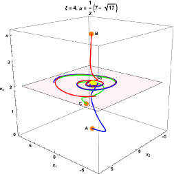
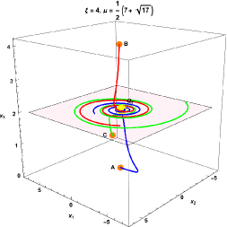
Figure 11: Projection of the dynamics of (186), (187) and (188) in the plane $x_{3}=2$ for $\mu=\frac{1}{2}(7\pm\sqrt{17})$ and $\xi=4.$ The origin dynamics of the plane $(x_{1},x_{2})=(0,0)$ (in yellow) shows that $Q_{3}=(0,0,\frac{1}{6}(r-2\mu+9))$ is an unstable focus. The spiral is generated from the initial conditions $A=(0.1,0.1)$, $B=(0.1,0.1,4)$ and $C=(1.9,-0.5,1).$

III.3.1 Alternative formulation of the dynamical system.

We define the variables

$$x=\frac{\dot{\phi}(t)}{\sqrt{6}H(t)},\quad y=\phi(t),\quad\Omega_{\Lambda}=\frac{\Lambda}{3H^{2}(t)},$$ (189)

that satisfy

$$(x+\sqrt{6}\xi y)^{2}+\xi y^{2}(1-6\xi)+\frac{(\mu-1)\left(1-\xi y^{2}\right)}{\alpha}+\Omega_{\Lambda}+\Omega_{m}=1,$$ (190)

where

$$\Omega_{m}=\frac{\rho_{m}}{3H^{2}},$$ (191)

which is the dimensionless energy density of matter, and $\Omega_{\Lambda}$ is interpreted as the energy density of the cosmological constant. The equation of state parameter of matter can be expressed in terms of these variables as

$$w =\left\{\alpha\left(\xi(12\xi+1)y^{2}-1\right)\left(-\alpha+\mu+\alpha x^{2}+\xi y\left(2\sqrt{6}\alpha x+y(\alpha-\mu+1)\right)+\alpha\Omega_{\Lambda}-1\right)\right\}^{-1}$$

$$\times\Bigg{\{}\alpha^{2}\left[x^{2}\left(\xi\left(y^{2}+12\right)-1\right)+2\sqrt{6}\xi xy\left(\xi y^{2}-1\right)+\xi y^{2}\left(-(12\xi+1)\Omega_{\Lambda}+\xi y^{2}-2\right)+\Omega_{\Lambda}+1\right]$$

$$+2\alpha\left(\xi y^{2}-1\right)\left[\mu\left(\xi y\left(\sqrt{6}x+y\right)-1\right)+\xi y\left(-\sqrt{6}x+12\xi y-3y\right)+3\right]$$

$$-(\mu-2)(\mu-1)\left(\xi y^{2}-1\right)^{2}\Bigg{\}}.$$ (192)

Introducing the new time derivative

$$\frac{df}{d\tau}\equiv\frac{1}{H}\frac{df}{dt},$$ (193)

we obtain the four-dimensional dynamical system

$$\alpha^{2}G\frac{dx}{d\tau} =-12\alpha^{2}\xi x^{3}+2\sqrt{6}\alpha\xi x^{2}y(-6\alpha\xi+\alpha+\mu-1)$$

$$+x\left(3\alpha\left(-\mu+8(\mu-1)\xi^{2}y^{2}+(\mu-3)\xi y^{2}+3\right)-(\mu-2)(\mu-1)\left(\xi y^{2}-1\right)\right)$$

$$+\sqrt{6}\xi y\left(\alpha^{2}+2\alpha(\mu-4)-(\mu-2)(\mu-1)\right)\left(\xi y^{2}-1\right),$$ (194)

$$\frac{dy}{d\tau} =\sqrt{6}x,$$ (195)

$$\alpha^{2}G\frac{d\Omega_{\Lambda}}{d\tau} =2\Omega_{\Lambda}\Bigg{\{}\alpha^{2}\left(-12\xi x^{2}+2\sqrt{6}\xi xy+3\xi(8\xi+1)y^{2}-3\right)$$

$$\quad\quad\quad\quad+2\alpha\left(\sqrt{6}(\mu-1)\xi xy+(\mu-4)\left(\xi y^{2}-1\right)\right)-(\mu-2)(\mu-1)\left(\xi y^{2}-1\right)\Bigg{\}},$$ (196)

$$\alpha G\frac{d\alpha}{d\tau} =3\alpha^{2}+2\alpha\mu-9\alpha-\mu^{2}+3\mu+\xi\Big{(}12\alpha^{2}x^{2}-2\sqrt{6}\alpha xy(\alpha+\mu-1)$$

$$\quad\quad+y^{2}\left(-2\alpha\mu-3(\alpha-3)\alpha+\mu^{2}-3\mu+2\right)\Big{)}+12(1-2\alpha)\alpha\xi^{2}y^{2}-2,$$ (197)

where

$$G:=(\xi(12\xi+1)y^{2}-1),$$ (198)

defined in phase space

$$(x+\sqrt{6}\xi y)^{2}+\xi y^{2}(1-6\xi)+\frac{(\mu-1)\left(1-\xi y^{2}\right)}{\alpha}+\Omega_{\Lambda}\leq 1$$ (199)

which corresponds to $\Omega_{m}\geq 0$.

We introduce temporal rescaling

$$f^{\prime}:=\alpha^{2}\frac{df}{d\tau},$$ (200)

that preserves the arrow of time. Sometimes, we use the time variable $\tau=\ln(a/a_{0})$ which is more convenient.

We obtain the equilibrium points with coordinates $(x,y,\Omega_{\Lambda},\alpha)$:

1. The line of equilibrium points $P_{1}(y_{c})$ with coordinates $\left(-\sqrt{6}\xi y_{c},y_{c},0,0\right)$ parameterized by $y_{c}\in\mathbb{R}$. The equation of state parameter is complex infinity. The eigenvalues are $\left\{0,-\frac{2(\mu-2)(\mu-1)\left(\xi y_{c}^{2}-1\right)}{\xi(12\xi+1)y_{c}^{2}-1},-\frac{(\mu-2)(\mu-1)\left(\xi y_{c}^{2}-1\right)}{\xi(12\xi+1)y_{c}^{2}-1},\frac{(\mu-2)(\mu-1)\left(\xi y_{c}^{2}-1\right)}{\xi(12\xi+1)y_{c}^{2}-1}\right\}$. The curve is a saddle because it has at least two eigenvalues with different signs.

2. The equilibrium point $P_{2}:\left(0,0,0,\frac{1}{6}(9-2\mu-r)\right)$. The equation of state parameter is $w=\frac{r+7}{4-4\mu}$. The eigenvalues are
   $\Big{\{}\frac{1}{3}(9-2\mu-r),\frac{1}{6}(-2\mu(8\mu+r-36)+9r-105),\frac{1}{36}\left(9(21-4\mu)\mu-9(\mu-3)r-279-s_{-}\right)$,
   $\frac{1}{36}\left(9(21-4\mu)\mu-9(\mu-3)r-279+s_{-}\right)\Big{\}}$ where $r=\sqrt{8\mu(2\mu-9)+105}$ and $s_{-}$ is the positive square root of $s_{-}^{2}=81(\mu(4\mu-21)+(\mu-3)r+31)^{2}-48\xi(\mu(\mu(2\mu(82\mu-933)+8355)-17361)+(\mu(5\mu(8\mu-75)+1209)-1413)r+14481)$.

   

   Figure 12: Real parts of the eigenvalues associated with $P_{2}$. This shows that the point is a sink if $(\mu,\xi)\in\Psi$, or a saddle (assuming $\xi\geq 0$).

   It is a saddle for $\Psi:=\left\{\mu\leq 0.463848,0<\xi\leq\frac{\mu\left(32\mu^{3}-8\mu^{2}(r+24)+6\mu(5r+83)-51r-567\right)+18(r+17)}{48(\mu-2)(\mu-1)(4(\mu-4)\mu+23)}\right\}\cup$
   $\left\{0.463848<\mu<1,0<\xi\leq\frac{\mu(2\mu(4\mu(4\mu+r-24)-15r+249)+51r-567)-18(r-17)}{48(\mu-2)(\mu-1)(4(\mu-4)\mu+23)}\right\}\cup$
   $\left\{\mu>2,0<\xi\leq\frac{\mu(2\mu(4\mu(4\mu+r-24)-15r+249)+51r-567)-18(r-17)}{48(\mu-2)(\mu-1)(4(\mu-4)\mu+23)}\right\}$. It is a source for
   $\frac{1}{48}\left(-\frac{\sqrt{8\mu(2\mu-9)+105}\left(\mu\left(8\mu^{2}-30\mu+51\right)-18\right)}{(\mu-2)(\mu-1)(4(\mu-4)\mu+23)}+\frac{38-20\mu}{4(\mu-4)\mu+23}+\frac{20}{\mu-2}-\frac{7}{\mu-1}+8\right)\leq\xi<0$. This case is discarded under the assumption $\xi\geq 0$. Figure 12 presents the real parts of the eigenvalues associated with $P_{2}$. This shows that the point is well for $(\mu,\xi)\in\Psi$, or a saddle (assuming $\xi\geq 0$).

3. The equilibrium point $P_{3}:\left(0,0,0,\frac{1}{6}(9-2\mu+r)\right)$. The equation of state parameter is $w=\frac{r-7}{4(\mu-1)}$. The eigenvalues are
   $\Big{\{}\frac{1}{3}(9-2\mu+r),\frac{1}{6}(2\mu(-8\mu+r+36)-3(3r+35)),\frac{1}{36}\left(9(21-4\mu)\mu+9(\mu-3)r-279-s_{+}\right)$,
   $\frac{1}{36}\left(9(21-4\mu)\mu+9(\mu-3)r-279+s_{+}\right)\Big{\}}$ where $r=\sqrt{8\mu(2\mu-9)+105}$ and $s_{+}$ is the positive square root of $s_{+}^{2}=81((21-4\mu)\mu+(\mu-3)r-31)^{2}+48\xi(\mu(\mu(2(933-82\mu)\mu-8355)+17361)+(\mu(5\mu(8\mu-75)+1209)-1413)r-14481)$. The point is always saddle, as shown in figure 13.

   

   Figure 13: Real parts of the eigenvalues associated with $P_{3}$. Hence, the point is a saddle.

4. The equilibrium point $P_{4}:\left(0,-\frac{1}{\sqrt{\xi}},0,\frac{1}{2}\right)$. The equation of state parameter is indeterminate. The eigenvalues are
   $\left\{-\frac{1}{2},1,\frac{1}{4}\left(2\mu-\sqrt{8\mu-19}-2\right),\frac{1}{4}\left(2\mu+\sqrt{8\mu-19}-2\right)\right\}$. The eigenvalue $1$ corresponds to the coordinate $\Omega_{\Lambda}$. It is always saddle for $\Omega_{\Lambda}\neq 0$. In the invariant set $\Omega_{\Lambda}=0$, they can be attractors if $\mu<1$. For $\mu=1$ the eigenvalues reduce to $-\frac{1}{2},\pm i\frac{\sqrt{11}}{4}$ and as shown in the lower panel of Figure 15 are spiral attractors. The analysis of this invariant set is presented in section III.4.

5. The equilibrium point $P_{5}:\left(0,\frac{1}{\sqrt{\xi}},0,\frac{1}{2}\right)$. The equation of state parameter is indeterminate. The eigenvalues are
   $\left\{-\frac{1}{2},1,\frac{1}{4}\left(2\mu-\sqrt{8\mu-19}-2\right),\frac{1}{4}\left(2\mu+\sqrt{8\mu-19}-2\right)\right\}$. The eigenvalue $1$ corresponds to the coordinate $\Omega_{\Lambda}$. It is always saddle for $\Omega_{\Lambda}\neq 0$. In the invariant set $\Omega_{\Lambda}=0$, they can be attractors if $\mu<1$. For $\mu=1$ the eigenvalues reduce to $-\frac{1}{2},\pm i\frac{\sqrt{11}}{4}$ and as shown in the lower panel of Figure 15 are spiral attractors. The analysis of this invariant set is presented in section III.4.

   There are additional points that cancel out the numerator and denominator, such as the following points:

6. The set $P_{6}(x_{c}):\left(x_{c},-\frac{1}{\sqrt{\xi}},\Omega_{\Lambda 0},0\right)$.

7. The line $P_{7}(x_{c}):\left(x_{c},-\frac{1}{\sqrt{\xi}},0,0\right)$. In both cases, the stability analysis of these point curves will be left for future research since it cannot be implemented with the techniques developed in this paper.

8. The line $P_{8}:\left(0,-\frac{1}{\sqrt{\xi}},\Omega_{\Lambda 0},0\right)$. The eigenvalues are
   $\left\{-2,4,\frac{\mu-\sqrt{\mu-1}-1}{\alpha}+o(1),\frac{\mu+\sqrt{\mu-1}-1}{\alpha}+o(1)\right\}$ when $\alpha\rightarrow 0$. Therefore, it is a saddle.

9. The point $P_{9}:\left(0,-\frac{1}{\sqrt{\xi}},0,0\right)$. The eigenvalues are
   
   $\left\{-2,4,\frac{\mu-\sqrt{\mu-1}-1}{\alpha}+o(1),\frac{\mu+\sqrt{\mu-1}-1}{\alpha}+o(1)\right\}$ when $\alpha\rightarrow 0$. Therefore, it is a saddle.

10. The set $P_{10}(x_{c}):\left(x_{c},\frac{1}{\sqrt{\xi}},\Omega_{\Lambda 0},0\right)$.

11. The line $P_{11}(x_{c}):\left(x_{c},\frac{1}{\sqrt{\xi}},0,0\right)$. In both cases, the stability analysis of these point curves will be left for future research since it cannot be implemented with the techniques developed in this paper.

12. The line $P_{12}:\left(0,\frac{1}{\sqrt{\xi}},\Omega_{\Lambda 0},0\right)$. The eigenvalues are
    
    $\left\{-2,4,\frac{\mu-\sqrt{\mu-1}-1}{\alpha}+o(1),\frac{\mu+\sqrt{\mu-1}-1}{\alpha}+o(1)\right\}$ when $\alpha\rightarrow 0$. Therefore, it is a saddle.

13. The point $P_{13}:\left(0,\frac{1}{\sqrt{\xi}},0,0\right)$. The eigenvalues are
    
    $\left\{-2,4,\frac{\mu-\sqrt{\mu-1}-1}{\alpha}+o(1),\frac{\mu+\sqrt{\mu-1}-1}{\alpha}+o(1)\right\}$ when $\alpha\rightarrow 0$. Therefore, it is a saddle. All have indeterminate parameters of the equation of state of matter.

14. The line $\left(0,-\frac{1}{\sqrt{\xi(12\xi+1)}},\Omega_{\Lambda 0},-\mu-\sqrt{\mu(2\mu-11)+18}+4\right)$.

15. The line $\left(0,-\frac{1}{\sqrt{\xi(12\xi+1)}},\Omega_{\Lambda 0},-\mu+\sqrt{\mu(2\mu-11)+18}+4\right)$.

16. The line $\left(0,\frac{1}{\sqrt{\xi(12\xi+1)}},\Omega_{\Lambda 0},-\mu-\sqrt{\mu(2\mu-11)+18}+4\right)$.

17. The line $\left(0,\frac{1}{\sqrt{\xi(12\xi+1)}},\Omega_{\Lambda 0},-\mu+\sqrt{\mu(2\mu-11)+18}+4\right)$. Stability can be determined numerically since the Jacobian matrix has infinite entries.

In these four cases, the stability analysis of these curves/sets of points will be left for future research since it cannot be implemented with the techniques developed in this paper. They all have infinitely complex parameters of the equation of state of matter.

Table 4: List of initial conditions used in the numerical integration of the system (III.3.1)-(III.3.1). As shown in figures 15 and 16, the values of $\xi$ considered are $1/6$ and $0.01$ while the values chosen for the parameter $\mu$ are $1$ and $1.1$.

Sol.	$x(0)$	$y(0)$	$\Omega_{\Lambda}(0)$	$\alpha(0)$
I	$0.01$	$\frac{1}{\sqrt{\xi+0.01}}$	$0.1$	$0.01$
II	$0.01$	$\frac{-1}{\sqrt{\xi+0.01}}$	$0.1$	$0.01$

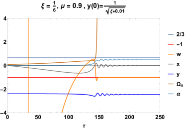
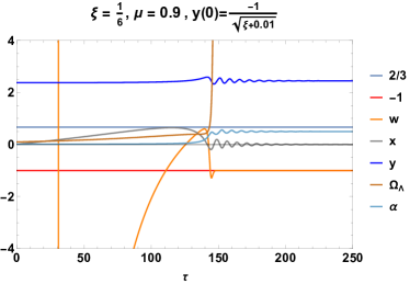
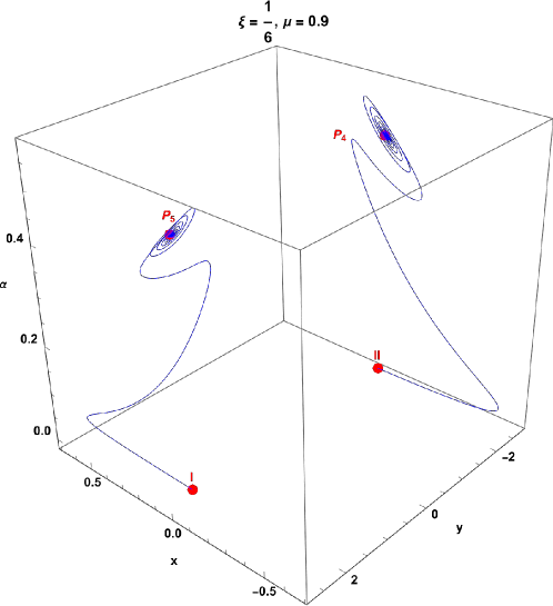
Figure 14: The upper panels show the numerical solution $x(\tau)$, $y(\tau)$, $\Omega_{\Lambda}(\tau)$ and $\alpha(\tau)$ of the system (III.3.1)-(III.3.1), as well as the effective equation of state of matter $w(\tau)$ defined in (III.3.1) for $\mu<1$. Two spiral orbits of the system, starting at the initial conditions labelled $I$ and $II$ in Table 4, asymptotically tend the equilibrium points $P_{4}$ and $P_{5}$.

The upper panels of figure 14 show the numerical solution $x(\tau)$, $y(\tau)$, $\Omega_{\Lambda}(\tau)$ and $\alpha(\tau)$ of the system (III.3.1)-(III.3.1), as well as the effective equation of state of matter $w(\tau)$ defined in (III.3.1) for $\mu<1$. Two spiral orbits of the system, starting at the initial conditions labelled $I$ and $II$ in Table 4, asymptotically tend the equilibrium points $P_{4}$ and $P_{5}$.

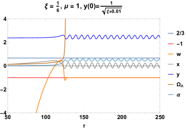
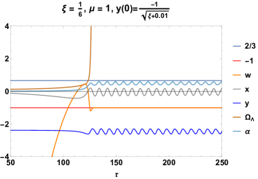
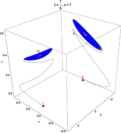
Figure 15: The upper panels show the numerical solution $x(\tau)$, $y(\tau)$, $\Omega_{\Lambda}(\tau)$ and $\alpha(\tau)$ of the system (III.3.1)-(III.3.1), as well as the effective equation of state of matter $w(\tau)$ defined in (III.3.1) for $\mu=1$. Two spiral orbits of the system, starting at the initial conditions labelled $I$ and $II$ in Table 4, asymptotically tend the equilibrium points $P_{4}$ and $P_{5}$.

In figure 15, the top panels show the numerical solution $x(\tau)$, $y(\tau)$, $\Omega_{\Lambda}(\tau)$ and $\alpha(\tau)$ of the system (III.3.1)-(III.3.1), as well as the effective equation of state of matter $w(\tau)$ defined in (III.3.1). The values of the parameters $\xi$ and $\mu$ are shown in the figure. In both cases, the equation of state $w(\tau)$ begins in a phantom regime ($w<-1$), crosses the matter-dominated region ($w=0$) and tends asymptotically to a regime of Sitter ($w=-1$). Two spiral orbits of the system starting at the initial conditions labelled $I$ and $II$ in Table 4 asymptotically tend the equilibrium points $P_{4}$ and $P_{5}$.

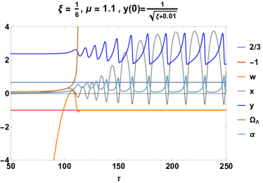
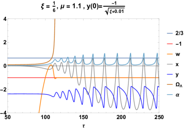
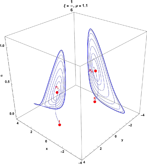
Figure 16: The upper panels show the numerical solution $x(\tau)$, $y(\tau)$, $\Omega_{\Lambda}(\tau)$ and $\alpha(\tau)$ of the system (III.3.1)-(III.3.1), as well as the effective state equation $w(\tau)$ defined in (III.3.1) for $\mu>1$. Two orbits starting at the initial conditions labelled $I$ and $II$ in Table 4 asymptotically tend to a limit cycle.

In figure 16 the top panels show the numerical solution $x(\tau)$, $y(\tau)$, $\Omega_{\Lambda}(\tau)$ and $\alpha(\tau)$ of the system (III.3.1)-(III.3.1), as well as the effective equation of state $w(\tau)$ defined in (III.3.1). The values of the parameters $\xi$ and $\mu$ are shown in the figure. In both cases, the equation of state $w(\tau)$ begins in a phantom regime ($w<-1$), crosses the matter-dominated region ($w=0$) and tends asymptotically to a regime of Sitter ($w=-1$). The oscillating behaviour of the functions $x(\tau)$, $y(\tau)$, $\Omega_{\Lambda}(\tau)$ and $\alpha(\tau)$ is still present but exhibits a greater amplitude compared to that shown in figure 15. Two orbits starting at the initial conditions labelled $I$ and $II$ in Table 4 tend asymptotically to a limit cycle.

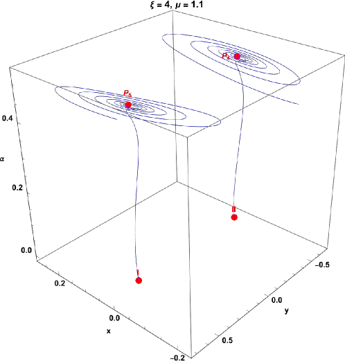
Figure 17: Dynamics in the invariant set $\Omega_{\Lambda}=0$ of the system (III.3.1)-(III.3.1) for the values of the parameters $\xi=4$ and $\mu=1.1$. Two orbits that begin at the initial conditions labelled $I$ and $II$ in Table 4 tend to the saddle points $P_{4}$ and $P_{5}$ and then form an unstable spiral centred on said points.

Figure 17 presents the dynamics in the invariant set $\Omega_{\Lambda}=0$ of the system (III.3.1)-(III.3.1) for the values of the parameters $\xi=4$ and $\mu=1.1$. Two orbits that begin at the initial conditions labelled $I$ and $II$ in Table 4 tend to the saddle points $P_{4}$ and $P_{5}$ and then form an unstable spiral centred on said points.

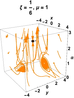
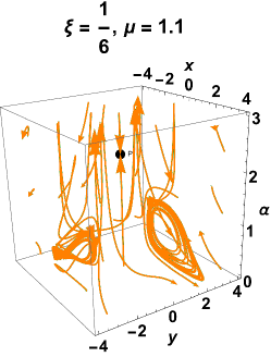
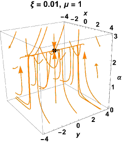
Figure 18: Phase diagrams for the system (III.3.1)-(III.3.1) for different values of the parameters $\xi$ and $\mu.$

Finally, in Figure 18 phase diagrams are presented for the (III.3.1)-(III.3.1) system for different values of the parameters $\xi$ and $\mu.$

In this section, we have numerically examined the invariant set $\Omega_{\Lambda}=0$ of the (III.3.1)-(III.3.1) system. However, to be able to characterize such an invariant set analytically, we will present a comprehensive analysis of dynamical systems in the section III.4.

III.4 Invariant set $\Omega_{\Lambda}=0$

Replacing $\Omega_{\Lambda}=0$ in (189), and defining the new variables

$$x=\frac{\dot{\phi}(t)}{\sqrt{6}H(t)},\quad y=\phi(t),$$ (201)

which satisfies

$$(x+\sqrt{6}\xi y)^{2}+\xi y^{2}(1-6\xi)+\frac{(\mu-1)\left(1-\xi y^{2}\right)}{\alpha}+\Omega_{m}=1,$$ (202)

where

$$\Omega_{m}=\frac{\rho_{m}}{3H^{2}}$$ (203)

is the dimensionless energy density of matter, we obtain an alternative formulation which describes the dynamics on the invariant set $\Omega_{\Lambda}=0$. The equation of state parameter of matter can be expressed in terms of the new variables as

$$w =\left\{\alpha\left(\xi(12\xi+1)y^{2}-1\right)\left(-\alpha+\mu+\alpha x^{2}+\xi y\left(2\sqrt{6}\alpha x+y(\alpha-\mu+1)\right)-1\right)\right\}^{-1}$$

$$\times\Bigg{\{}\alpha^{2}\left[x^{2}\left(\xi\left(y^{2}+12\right)-1\right)+2\sqrt{6}\xi xy\left(\xi y^{2}-1\right)+\xi y^{2}\left(\xi y^{2}-2\right)+1\right]$$

$$+2\alpha\left(\xi y^{2}-1\right)\left[\mu\left(\xi y\left(\sqrt{6}x+y\right)-1\right)+\xi y\left(-\sqrt{6}x+12\xi y-3y\right)+3\right]$$

$$-(\mu-2)(\mu-1)\left(\xi y^{2}-1\right)^{2}\Bigg{\}}.$$ (204)

Introducing the derivative (193), we obtain the three-dimensional dynamical system

$$\alpha^{2}G\frac{dx}{d\tau} =-12\alpha^{2}\xi x^{3}+2\sqrt{6}\alpha\xi x^{2}y(-6\alpha\xi+\alpha+\mu-1)$$

$$+x\left(3\alpha\left(-\mu+8(\mu-1)\xi^{2}y^{2}+(\mu-3)\xi y^{2}+3\right)-(\mu-2)(\mu-1)\left(\xi y^{2}-1\right)\right)$$

$$+\sqrt{6}\xi y\left(\alpha^{2}+2\alpha(\mu-4)-(\mu-2)(\mu-1)\right)\left(\xi y^{2}-1\right),$$ (205)

$$\frac{dy}{d\tau} =\sqrt{6}x,$$ (206)

$$\alpha G\frac{d\alpha}{d\tau} =3\alpha^{2}+2\alpha\mu-9\alpha-\mu^{2}+3\mu+\xi\Big{(}12\alpha^{2}x^{2}-2\sqrt{6}\alpha xy(\alpha+\mu-1)$$

$$\quad\quad+y^{2}\left(-2\alpha\mu-3(\alpha-3)\alpha+\mu^{2}-3\mu+2\right)\Big{)}+12(1-2\alpha)\alpha\xi^{2}y^{2}-2,$$ (207)

where

$$G:=(\xi(12\xi+1)y^{2}-1),$$ (208)

defined on the phase space

$$(x+\sqrt{6}\xi y)^{2}+\xi y^{2}(1-6\xi)+\frac{(\mu-1)\left(1-\xi y^{2}\right)}{\alpha}\leq 1$$ (209)

which corresponds to $\Omega_{m}\geq 0$.

Introducing the time-rescaling (200) which preserves the arrow of time; we obtain the system

$$x^{\prime} =\frac{1}{\xi(12\xi+1)y^{2}-1}\Bigg{[}-12\alpha^{2}\xi x^{3}+2\sqrt{6}\alpha\xi x^{2}y(-6\alpha\xi+\alpha+\mu-1)$$

$$+x\left(3\alpha\left(-\mu+8(\mu-1)\xi^{2}y^{2}+(\mu-3)\xi y^{2}+3\right)-(\mu-2)(\mu-1)\left(\xi y^{2}-1\right)\right)$$

$$+\sqrt{6}\xi y\left(\alpha^{2}+2\alpha(\mu-4)-(\mu-2)(\mu-1)\right)\left(\xi y^{2}-1\right)\Bigg{]},$$ (210)

$$y^{\prime} =\sqrt{6}\alpha^{2}x,$$ (211)

$$\alpha^{\prime} =\frac{\alpha}{\xi(12\xi+1)y^{2}-1}\Bigg{[}3\alpha^{2}+2\alpha\mu-9\alpha-\mu^{2}+3\mu+12(1-2\alpha)\alpha\xi^{2}y^{2}-2$$

$$+\xi\left(12\alpha^{2}x^{2}-2\sqrt{6}\alpha xy(\alpha+\mu-1)+y^{2}\left(-2\alpha\mu-3(\alpha-3)\alpha+\mu^{2}-3\mu+2\right)\right)\Bigg{]}.$$ (212)

sometimes is more useful to use the time variable $\tau=\ln(a/a_{0})$.

The equilibrium points of system (210), (211) y (212) in the coordinates $(x,y,\alpha)$ are:

1. The equilibrium point curve $P_{1}:\left(-\sqrt{6}\xi y_{c},y_{c},0\right)$ parameterized by $y_{c}\in\mathbb{R}$. The equation of state parameter is complex infinity. The eigenvalues are
   $\left\{0,-\frac{(\mu-2)(\mu-1)\left(\xi y^{2}-1\right)}{\xi(12\xi+1)y^{2}-1},\frac{(\mu-2)(\mu-1)\left(\xi y^{2}-1\right)}{\xi(12\xi+1)y^{2}-1}\right\}$. The curve is a saddle because it has at least two eigenvalues with different signs.

2. The equilibrium point $P_{2}:\left(0,0,\frac{1}{6}(9-2\mu-r)\right)$. There exists ($\alpha>0$) for $1\leq\mu\leq 2$. The eigenvalues are $\Big{\{}\frac{1}{6}\left(-2\mu\left(8\mu+r-36\right)+9r-105\right)$,
   $\frac{1}{72}\left(-72\mu^{2}-u_{-}-18r\mu+378\mu+54r-558\right)$,
   $\frac{1}{72}\left(-72\mu^{2}+u_{-}-18r\mu+378\mu+54r-558\right)\Big{\}}$. Where $r=\sqrt{8\mu(2\mu-9)+105}$ and $u_{-}$ is the positive square root of
   $u_{-}^{2}=324\left(\mu\left(4\mu+r-21\right)-3r+31\right)^{2}\newline -192\left(\mu\left(3\left(403r-5787\right)+\mu\left(2\mu\left(82\mu+20r-933\right)-375r+8355\right)\right)-1413r+14481\right)\xi$. The critical point is a saddle in its existence interval, as shown in the figure 19.

   

   Figure 19: Eigenvalues of $P_{2}$ showing that the point is a saddle.

   The equation of state parameter is $w=\frac{-2\mu\left(r+9\right)+3r+35}{4\mu(2\mu-3)-4}$.

3. The equilibrium point $P_{3}:\left(0,0,\frac{1}{6}(9-2\mu+r)\right)$. The eigenvalues are
   $\Big{\{}\frac{1}{6}\left(2\mu\left(-8\mu+r+36\right)-3\left(3r+35\right)\right)$,
   $\frac{1}{72}\left(-u_{+}-72\mu^{2}+18r\mu+378\mu-54r-558\right)$,
   $\frac{1}{72}\left(u_{+}-72\mu^{2}+18r\mu+378\mu-54r-558\right)\Big{\}}$, where $r=\sqrt{8\mu(2\mu-9)+105}$ and $u_{+}$ is the positive square root of $u_{+}^{2}=324\left(4\mu^{2}-\left(r+21\right)\mu+3r+31\right)^{2}\newline +192\left(\mu\left(3\left(403r+5787\right)+\mu\left(2\mu\left(-82\mu+20r+933\right)-15\left(25r+557\right)\right)\right)-9\left(157r+1609\right)\right)\xi$. $P_{3}$ is a sink for $\left\{\mu>2,0<\xi\leq\frac{1}{48}\right\}\cup\left\{\mu=1,0<\xi\leq\frac{27}{154}\right\}\cup\left\{\mu=2,0<\xi\leq\frac{27}{280}\right\}\newline \cup\left\{\mu+\frac{1}{4}\left(-5-\frac{9}{\sqrt[3]{58+\sqrt{4093}}}+\sqrt[3]{58+\sqrt{4093}}\right)=0,0<\xi\leq-\frac{27(\mu-3)}{4\left(2\mu^{3}-3\mu^{2}-12\mu+90\right)}\right\}\newline \cup\left\{0<\mu<\frac{1}{4}\left(5-\frac{9}{\sqrt[3]{\sqrt{4093}-58}}+\sqrt[3]{\sqrt{4093}-58}\right),0<\xi\leq\frac{1}{48}\right\}\newline \cup\left\{\frac{1}{4}\left(5-\frac{9}{\sqrt[3]{\sqrt{4093}-58}}+\sqrt[3]{\sqrt{4093}-58}\right)<\mu<1,0<\xi\leq\frac{1}{48}\right\}$.

   It is a saddle otherwise.

   The equation of state parameter is $w=\frac{2\mu\left(r-9\right)-3r+35}{4\mu(2\mu-3)-4}$.

4. The equilibrium point $P_{4}:\left(0,-\frac{1}{\sqrt{\xi}},\frac{1}{2}\right)$. The eigenvalues are
   $\Big{\{}-\frac{1}{2},\frac{1}{4}\left(2\mu-\sqrt{8\mu-19}-2\right),\frac{1}{4}\left(2\mu+\sqrt{8\mu-19}-2\right)\Big{\}}$. The equation of state parameter is $w=\frac{1}{24\left(\xi^{3/2}+\xi\right)}$. The point is sink for $0<\mu<1$ and $\xi>0$, and is saddle for $\mu>1$. As shown in the figure 17.

5. The equilibrium point $P_{5}:\left(0,\frac{1}{\sqrt{\xi}},\frac{1}{2}\right)$. The eigenvalues are
   $\Big{\{}-\frac{1}{2},\frac{1}{4}\left(2\mu-\sqrt{8\mu-19}-2\right),\frac{1}{4}\left(2\mu+\sqrt{8\mu-19}-2\right)\Big{\}}$. The equation of state parameter is $w=\frac{1}{24\left(\xi^{3/2}+\xi\right)}$. The point is sink for $0<\mu<1$ and $\xi>0$, and is saddle for $\mu>1$. As shown in figure 17.

6. The equilibrium point $P_{7}:\left(x_{c},-\frac{1}{\sqrt{\xi}},0\right)$.

7. The equilibrium point $P_{9}:\left(0,-\frac{1}{\sqrt{\xi}},0\right)$. The equation of state parameter is $w=0$.

8. The equilibrium point $P_{11}:\left(x_{c},\frac{1}{\sqrt{\xi}},0\right)$.

9. The equilibrium point $P_{13}:\left(0,\frac{1}{\sqrt{\xi}},0\right)$. The equation of state parameter is $w=0$.

   Due to the complexity of the stability analysis of these four points, it will be left for future research since it cannot be implemented with the techniques developed in this paper.

10. The equilibrium points $\left(0,-\frac{1}{\sqrt{\xi(12\xi+1)}},-\mu-\sqrt{\mu(2\mu-11)+18}+4\right)$.

11. The equilibrium points $\left(0,-\frac{1}{\sqrt{\xi(12\xi+1)}},-\mu+\sqrt{\mu(2\mu-11)+18}+4\right)$.

12. The equilibrium points $\left(0,\frac{1}{\sqrt{\xi(12\xi+1)}},-\mu-\sqrt{\mu(2\mu-11)+18}+4\right)$.

13. The equilibrium points $\left(0,\frac{1}{\sqrt{\xi(12\xi+1)}},-\mu+\sqrt{\mu(2\mu-11)+18}+4\right)$.

In all four cases, the equation of state parameter is complex and infinite. Due to the complexity of the stability analysis of this set of equilibrium points, numerical solution methods can be used. The stability analysis of these four points is very complex, so it will be left for future research since it cannot be implemented with the techniques developed in this paper.

III.4.1 Asymptotic expansions for $\varepsilon:=\mu-1\rightarrow 0$

Next, we will study the perturbation problem related to the study of the phase portrait of a system of differential equations

$$\dot{x}=X(x;\varepsilon),\quad x\in\mathbb{R}^{3},\quad\varepsilon\sim 0$$ (213)

in a neighbourhood of the origin, where the unperturbed vector field is $X(x;0)$ (Fenichel,, 1979; Kevorkian,, 1981; Fusco and Hale,, 1988; Dumortier and Roussarie,, 1995; Holmes,, 2013; Verhulst,, 2000; Berglund and Gentz,, 2006).

To obtain asymptotic expansions for $\mu\rightarrow 1$, the reparametrization $\varepsilon:=\mu-1$ is introduced and the limit $\varepsilon\rightarrow 0$ is analyzed using the asymptotic expansion

$$\rho=\rho_{0}+\varepsilon\rho_{1}+\mathcal{O}(\varepsilon^{2}),\;p=p_{0}+\varepsilon p_{1}+\mathcal{O}(\varepsilon^{2}),\;H=H_{0}+\varepsilon H_{1}+\mathcal{O}(\varepsilon^{2}),\;\phi=\phi_{0}+\varepsilon\phi_{1}+\mathcal{O}(\varepsilon^{2}).$$

After making the substitution in the field equations and comparing the coefficients with equal powers of $\varepsilon$, the following is obtained.

At order $0$ we have the equations

$$\dot{H_{0}}=\frac{2t\xi\dot{\phi_{0}}^{2}-2t\xi H_{0}\phi_{0}\dot{\phi_{0}}+3H_{0}\left(-\xi((8\xi t+t)H_{0}-2)\phi_{0}^{2}+tH_{0}-2\right)}{t\left(\xi(12\xi+1)\phi_{0}^{2}-1\right)},$$ (214)

$$\ddot{\phi_{0}}=\frac{-12t\xi^{2}\phi_{0}\dot{\phi_{0}}^{2}-3tH_{0}\left(\xi(8\xi+1)\phi_{0}^{2}-1\right)\dot{\phi_{0}}+6\xi H_{0}(tH_{0}-6)\phi_{0}\left(\xi\phi_{0}^{2}-1\right)}{t\left(\xi(12\xi+1)\phi_{0}^{2}-1\right)},$$ (215)

and the auxiliary equation

$$\dot{\rho_{0}}=\frac{3H_{0}}{t\left(\xi(12\xi+1)\phi_{0}^{2}-1\right)}\Bigg{[}t\left(\xi(6\xi+1)\phi_{0}^{2}+6\xi-1\right)\dot{\phi_{0}}^{2}+12t\xi H_{0}\phi_{0}\left(\xi(6\xi+1)\phi_{0}^{2}-1\right)\dot{\phi_{0}}$$

$$+6H_{0}\left(\xi\phi_{0}^{2}-1\right)\left(\xi(12\xi+(6\xi t+t)H_{0}-2)\phi_{0}^{2}-tH_{0}+2\right)\Bigg{]},$$ (216)

and the constraints

$$\rho_{0}=3\left(1-\xi\phi_{0}^{2}\right)H_{0}^{2}-6\xi\phi_{0}\dot{\phi_{0}}H_{0}-\frac{1}{2}\dot{\phi_{0}}^{2}-\Lambda,$$ (217)

$$p_{0}=-\frac{1}{2t\left(\xi(12\xi+1)\phi_{0}^{2}-1\right)}\Bigg{[}6tH_{0}^{2}\left(\xi\phi_{0}^{2}-1\right)^{2}+12H_{0}\left(\xi\phi_{0}\left(2(6\xi-1)\phi_{0}+t\dot{\phi_{0}}\right)+2\right)\left(\xi\phi_{0}^{2}-1\right)$$

$$+t\left(\xi\phi_{0}^{2}+12\xi-1\right)\dot{\phi_{0}}^{2}+2t\Lambda\left(1-\xi(12\xi+1)\phi_{0}^{2}\right)\Bigg{]}.$$ (218)

At order $1$ we have the equations

$$\dot{H_{1}}=\frac{1}{t^{2}\left(\xi(12\xi+1)\phi_{0}^{2}-1\right)^{2}}\Bigg{[}-24\xi^{2}H_{0}^{2}\phi_{0}\phi_{1}t^{2}+4\xi\left(\xi(12\xi+1)\phi_{0}^{2}-1\right)\dot{\phi_{0}}\dot{\phi_{1}}t^{2}$$

$$-2H_{1}\left(\xi(12\xi+1)\phi_{0}^{2}-1\right)\left(\xi\phi_{0}\left(t\dot{\phi_{0}}-3\phi_{0}\right)+3\right)t$$

$$+2H_{0}\Bigg{(}3tH_{1}\left(\xi\phi_{0}^{2}\left(-\xi(8\xi+1)(12\xi+1)\phi_{0}^{2}+20\xi+2\right)-1\right)$$

$$+\xi\Big{\{}-\xi(12\xi+1)\phi_{0}^{4}-t\xi(12\xi+1)\dot{\phi_{1}}\phi_{0}^{3}+\left(t(12\xi+1)\phi_{1}\dot{\phi_{0}}\xi+12\xi+2\right)\phi_{0}^{2}$$

$$+\left(72\xi\phi_{1}+t\dot{\phi_{1}}\right)\phi_{0}+t\phi_{1}\dot{\phi_{0}}\Big{\}}-1\Bigg{)}t$$

$$+2\xi(6\xi+1)\phi_{0}^{2}+\xi\phi_{0}\left(2t\dot{\phi_{0}}-\xi(12\xi+1)\left(\phi_{0}^{3}+2t\dot{\phi_{0}}\phi_{0}^{2}+4t^{2}\phi_{1}\dot{\phi_{0}}^{2}\right)\right)-1\Bigg{]},$$ (219)

$$\ddot{\phi_{1}}=\frac{1}{t^{2}\left(\xi(12\xi+1)\phi_{0}^{2}-1\right)^{2}}\Bigg{[}6\xi^{3}(12\xi+1)(2t(H_{0}+(tH_{0}-3)H_{1})+1)\phi_{0}^{5}$$

$$+t\xi^{2}(12\xi+1)\left(6t\xi\phi_{1}H_{0}^{2}-36\xi\phi_{1}H_{0}-3t(8\xi+1)\dot{\phi_{1}}H_{0}+(24\xi-3t(8\xi+1)H_{1}+1)\dot{\phi_{0}}\right)\phi_{0}^{4}$$

$$+12\xi^{2}\left(-2\xi(12\xi+1)\dot{\phi_{0}}\dot{\phi_{1}}t^{2}-(6\xi+1)(2t(H_{0}+(tH_{0}-3)H_{1})+1)\right)\phi_{0}^{3}$$

$$+2t\xi\Big{\{}6t\xi(6\xi-1)\phi_{1}H_{0}^{2}+3\left(12(1-6\xi)\xi\phi_{1}+t(10\xi+1)\dot{\phi_{1}}\right)H_{0}$$

$$+\dot{\phi_{0}}\left(6t(12\xi+1)\phi_{1}\dot{\phi_{0}}\xi^{2}-18\xi+3t(10\xi+1)H_{1}-1\right)\Big{\}}\phi_{0}^{2}$$

$$+6\xi\left(2t\left(-3H_{1}+H_{0}\left(tH_{1}-2t\xi\phi_{1}\dot{\phi_{0}}+1\right)+2t\xi\dot{\phi_{0}}\dot{\phi_{1}}\right)+1\right)\phi_{0}$$

$$+t\left(6t\xi\phi_{1}H_{0}^{2}-3\left(12\xi\phi_{1}+t\dot{\phi_{1}}\right)H_{0}+\dot{\phi_{0}}\left(12t\phi_{1}\dot{\phi_{0}}\xi^{2}-3tH_{1}+1\right)\right)\Bigg{]},$$ (220)

the auxiliary equation

$$\dot{\rho_{1}}=\frac{1}{t^{2}\left(\xi(12\xi+1)\phi_{0}^{2}-1\right)^{2}}\Bigg{[}36t^{2}\xi\phi_{0}\left(\xi(6\xi+1)\left(\xi(12\xi+1)\phi_{0}^{2}-2\right)\phi_{0}^{2}-6\xi+1\right)\phi_{1}H_{0}^{3}$$

$$+3t\Bigg{(}18tH_{1}\left(\xi\phi_{0}^{2}-1\right)\left(\xi(6\xi+1)\phi_{0}^{2}-1\right)\left(\xi(12\xi+1)\phi_{0}^{2}-1\right)$$

$$+\xi\Bigg{\{}\xi^{2}(1-36\xi(16\xi+1))\phi_{0}^{6}+12\xi^{2}(12\xi+1)\left(2(6\xi-1)\phi_{1}+t(6\xi+1)\dot{\phi_{1}}\right)\phi_{0}^{5}$$

$$+3\xi\left(24\xi(8\xi+1)+4t\xi(6\xi+1)(12\xi+1)\phi_{1}\dot{\phi_{0}}-1\right)\phi_{0}^{4}$$

$$-24\xi\left(2(6\xi-1)\phi_{1}+t(9\xi+1)\dot{\phi_{1}}\right)\phi_{0}^{3}-3\left(8t(3\xi+1)\phi_{1}\dot{\phi_{0}}\xi+12\xi-1\right)\phi_{0}^{2}$$

$$+12\left((36\xi-2)\phi_{1}+t\dot{\phi_{1}}\right)\phi_{0}+12t\phi_{1}\dot{\phi_{0}}\Bigg{\}}-1\Bigg{)}H_{0}^{2}$$

$$+3\Bigg{(}2\left(\xi(6\xi+1)\phi_{0}^{2}+6\xi-1\right)\left(\xi(12\xi+1)\phi_{0}^{2}-1\right)\dot{\phi_{0}}\dot{\phi_{1}}t^{2}$$

$$+24H_{1}\left(\xi(12\xi+1)\phi_{0}^{2}-1\right)\left(\xi\phi_{0}\left(\phi_{0}\left(\xi(6\xi-1)\phi_{0}^{2}-6\xi+2\right)+t\left(\xi(6\xi+1)\phi_{0}^{2}-1\right)\dot{\phi_{0}}\right)-1\right)t$$

$$+\xi\phi_{0}\Bigg{\{}\xi^{2}(12(5-24\xi)\xi+7)\phi_{0}^{5}+3\xi(8\xi(12\xi-5)-7)\phi_{0}^{3}+3(20\xi+7)\phi_{0}$$

$$-144t^{2}\xi^{2}\phi_{1}\dot{\phi_{0}}^{2}+2t\left(\xi\left(\left(\xi-144\xi^{3}\right)\phi_{0}^{2}-2\right)\phi_{0}^{2}+1\right)\dot{\phi_{0}}\Bigg{\}}-7\Bigg{)}H_{0}$$

$$+t(3tH_{1}-1)\left(\xi(6\xi+1)\phi_{0}^{2}+6\xi-1\right)\left(\xi(12\xi+1)\phi_{0}^{2}-1\right)\dot{\phi_{0}}^{2}\Bigg{]},$$ (221)

and the constraints

$$\rho_{1}=-6\xi\phi_{0}\phi_{1}H_{0}^{2}-\frac{3(2tH_{1}-1)\left(\xi\phi_{0}^{2}-1\right)H_{0}}{t}-6\xi(H_{1}\phi_{0}+H_{0}\phi_{1})\dot{\phi_{0}}-\left(6\xi H_{0}\phi_{0}+\dot{\phi_{0}}\right)\dot{\phi_{1}},$$ (222)

$$p_{1}=-\frac{1}{t^{2}\left(\xi(12\xi+1)\phi_{0}^{2}-1\right)^{2}}\Bigg{[}-144t^{2}\phi_{0}\phi_{1}\dot{\phi_{0}}^{2}\xi^{3}+6t^{2}H_{0}^{2}\phi_{0}\left(\xi\phi_{0}^{2}-1\right)\left(\xi(12\xi+1)\phi_{0}^{2}+12\xi-1\right)\phi_{1}\xi$$

$$+6t\phi_{0}\left(\xi\phi_{0}^{2}-1\right)\left(\xi(12\xi+1)\phi_{0}^{2}-1\right)\dot{\phi_{0}}\xi+3\left(\xi\phi_{0}^{2}-1\right)^{2}\left(\xi(12\xi+1)\phi_{0}^{2}-1\right)$$

$$+6tH_{1}\left(\xi\phi_{0}^{2}-1\right)\left(\xi(12\xi+1)\phi_{0}^{2}-1\right)\left(\xi\phi_{0}\left(2(6\xi-1)\phi_{0}+t\dot{\phi_{0}}\right)+2\right)$$

$$+t^{2}\left(\xi\phi_{0}^{2}+12\xi-1\right)\left(\xi(12\xi+1)\phi_{0}^{2}-1\right)\dot{\phi_{0}}\dot{\phi_{1}}+6tH_{0}\Big{\{}tH_{1}\left(\xi(12\xi+1)\phi_{0}^{2}-1\right)\left(\xi\phi_{0}^{2}-1\right)^{2}$$

$$+\xi\Bigg{(}\xi^{2}(12\xi+1)\phi_{0}^{6}+\xi^{2}(12\xi+1)\left(4(6\xi-1)\phi_{1}+t\dot{\phi_{1}}\right)\phi_{0}^{5}+\xi\left(t\xi(12\xi+1)\phi_{1}\dot{\phi_{0}}-3(8\xi+1)\right)\phi_{0}^{4}$$

$$-2\xi\left(4(6\xi-1)\phi_{1}+t(6\xi+1)\dot{\phi_{1}}\right)\phi_{0}^{3}+\left(2t(6\xi-1)\phi_{1}\dot{\phi_{0}}\xi+12\xi+3\right)\phi_{0}^{2}$$

$$+\left((72\xi-4)\phi_{1}+t\dot{\phi_{1}}\right)\phi_{0}+t\phi_{1}\dot{\phi_{0}}\Bigg{)}-1\Big{\}}\Bigg{]}.$$ (223)

For simplicity, we will solve the case $\xi=0$.

At order $0$ we have the equations

$$\dot{H_{0}}=-\frac{3H_{0}(-2+tH_{0})}{t},$$ (224)

$$\dot{\rho_{0}}=-\frac{3H_{0}\left(-6H_{0}(2-tH_{0})-t\dot{\phi}^{2}\right)}{t},$$ (225)

$$\ddot{\phi_{0}}=-3H_{0}\dot{\phi_{0}}.$$ (226)

and the constraints

$$\rho_{0}=3H_{0}^{2}-\Lambda-\frac{1}{2}\dot{\phi_{0}}^{2},$$ (227)

$$p_{0}=\frac{6tH_{0}^{2}-24H_{0}+2\Lambda t-t\dot{\phi_{0}}^{2}}{2t}.$$ (228)

At order $1$ we have the equations

$$\dot{H_{1}}=\frac{-1+6tH_{1}+2tH_{0}(-1-3tH_{1})}{t^{2}},$$ (229)

$$\dot{\rho_{1}}=\frac{1}{t^{2}}\left(3tH_{0}^{2}(-1-18tH_{1})+t(-1+3tH_{1})\dot{\phi_{0}}^{2}+3H_{0}\left(-7+24tH_{1}+2t^{2}\dot{\phi_{0}}\dot{\phi_{1}}\right)\right),$$ (230)

$$\ddot{\phi_{1}}=\frac{(1-3tH_{1})\dot{\phi_{0}}-3tH_{0}\dot{\phi_{1}}}{t}.$$ (231)

and the constraints

$$\rho_{1}=\frac{3H_{0}(2tH_{1}-1)}{t}-\dot{\phi_{0}}\dot{\phi_{1}},$$ (232)

$$p_{1}=-\frac{6tH_{0}(-tH_{1}-1)+12tH_{1}+t^{2}\dot{\phi_{0}}\dot{\phi_{1}}-3}{t^{2}}.$$ (233)

Solving the resulting systems we obtain

$$H_{0}(t)=\frac{7t^{6}}{3t^{7}+7c_{1}},$$ (234)

$$H_{1}(t)=\frac{-51t^{14}+7c_{2}t^{7}-980c_{1}\ln(t)t^{7}+49c_{1}{}^{2}}{7t\left(3t^{7}+7c_{1}\right){}^{2}},$$ (235)

$$\rho_{0}(t)=\frac{147t^{12}}{\left(3t^{7}+7c_{1}\right){}^{2}}-\frac{c_{3}{}^{2}}{2\left(3t^{7}+7c_{1}\right){}^{2}}+c_{4},$$ (236)

where $c_{1}$, $c_{2}$, $c_{3}$ y $c_{4}$ are integration constants.

$$\phi_{0}(t)=c_{5}+\frac{c_{3}}{7\sqrt[7]{3}7^{\frac{6}{7}}c_{1}{}^{\frac{6}{7}}}\Bigg{[}-2\sin\left(\frac{\pi}{7}\right)\tan^{-1}\left(\cot\left(\frac{\pi}{7}\right)-\frac{\sqrt[7]{\frac{3}{7}}t\csc\left(\frac{\pi}{7}\right)}{\sqrt[7]{c_{1}}}\right)$$

$$+\ln\left(\sqrt[7]{3}7^{\frac{6}{7}}t+7\sqrt[7]{c_{1}}\right)-\cos\left(\frac{\pi}{7}\right)\ln\left(3^{\frac{2}{7}}7^{\frac{5}{7}}t^{2}-2\sqrt[7]{3}7^{\frac{6}{7}}\sqrt[7]{c_{1}}\cos\left(\frac{\pi}{7}\right)t+7c_{1}{}^{\frac{2}{7}}\right)$$

$$+\ln\left(3^{\frac{2}{7}}7^{\frac{5}{7}}t^{2}+2\sqrt[7]{3}7^{\frac{6}{7}}\sqrt[7]{c_{1}}\sin\left(\frac{3\pi}{14}\right)t+7c_{1}{}^{\frac{2}{7}}\right)\sin\left(\frac{3\pi}{14}\right)$$

$$-\ln\left(3^{\frac{2}{7}}7^{\frac{5}{7}}t^{2}-2\sqrt[7]{3}7^{\frac{6}{7}}\sqrt[7]{c_{1}}\sin\left(\frac{\pi}{14}\right)t+7c_{1}{}^{\frac{2}{7}}\right)\sin\left(\frac{\pi}{14}\right)$$

$$+2\tan^{-1}\left(\frac{\sqrt[7]{\frac{3}{7}}\sec\left(\frac{3\pi}{14}\right)t}{\sqrt[7]{c_{1}}}+\tan\left(\frac{3\pi}{14}\right)\right)\cos\left(\frac{3\pi}{14}\right)$$

$$+2\tan^{-1}\left(\frac{\sqrt[7]{\frac{3}{7}}t\sec\left(\frac{\pi}{14}\right)}{\sqrt[7]{c_{1}}}-\tan\left(\frac{\pi}{14}\right)\right)\cos\left(\frac{\pi}{14}\right)\Bigg{]},$$ (237)

$$\rho_{1}(t)=-\frac{1}{7\left(3t^{7}+7c_{1}\right){}^{3}}\Bigg{[}-189c_{7}t^{21}+3465t^{19}-1323c_{1}c_{7}t^{14}+294(21c_{1}-c_{2})t^{12}$$

$$+21\left(c_{3}c_{6}-147c_{1}{}^{2}c_{7}\right)t^{7}+5145c_{1}{}^{2}t^{5}+14c_{1}c_{3}{}^{2}+c_{2}c_{3}{}^{2}+49c_{1}c_{3}c_{6}-2401c_{1}{}^{3}c_{7}$$

$$+4\left(10290c_{1}t^{12}+18c_{3}{}^{2}t^{7}+7c_{1}c_{3}{}^{2}\right)\ln(t)\Bigg{]},$$ (238)

where $c_{5}$, $c_{6}$ y $c_{7}$ are integration constants.

Finally,

$$\phi_{1}(t)=-\frac{9c_{3}\,{}_{3}F_{2}\left(\frac{8}{7},\frac{8}{7},2;\frac{15}{7},\frac{15}{7};-\frac{3t^{7}}{7c_{1}}\right)t^{8}}{2744c_{1}{}^{2}}+\frac{9c_{3}\,{}_{2}F_{1}\left(\frac{8}{7},2;\frac{15}{7};-\frac{3t^{7}}{7c_{1}}\right)\ln(t)t^{8}}{343c_{1}{}^{2}}+\frac{c_{2}c_{3}t}{343c_{1}\left(3t^{7}+7c_{1}\right)}+\frac{2c_{3}t}{49\left(3t^{7}+7c_{1}\right)}$$

$$-\frac{4c_{3}\,{}_{3}F_{2}\left(\frac{1}{7},\frac{1}{7},2;\frac{8}{7},\frac{8}{7};-\frac{3t^{7}}{7c_{1}}\right)t}{49c_{1}}+\frac{4c_{3}\,{}_{2}F_{1}\left(\frac{1}{7},2;\frac{8}{7};-\frac{3t^{7}}{7c_{1}}\right)\ln(t)t}{49c_{1}}+c_{8}+\frac{2\left(\frac{3}{7}\right)^{\frac{6}{7}}c_{2}c_{3}\ln\left(\sqrt[7]{3}7^{\frac{6}{7}}t+7\sqrt[7]{c_{1}}\right)}{2401c_{1}{}^{\frac{13}{7}}}$$

$$+\frac{4\left(\frac{3}{7}\right)^{\frac{6}{7}}c_{3}\ln\left(\sqrt[7]{3}7^{\frac{6}{7}}t+7\sqrt[7]{c_{1}}\right)}{343c_{1}{}^{\frac{6}{7}}}+\frac{c_{6}\ln\left(\sqrt[7]{3}7^{\frac{6}{7}}t+7\sqrt[7]{c_{1}}\right)}{7\sqrt[7]{3}7^{\frac{6}{7}}c_{1}{}^{\frac{6}{7}}}-\frac{2\left(\frac{3}{7}\right)^{\frac{6}{7}}c_{2}c_{3}\cos^{2}\left(\frac{\pi}{14}\right)\ln\left(3^{\frac{2}{7}}7^{\frac{5}{7}}t^{2}-2\sqrt[7]{3}7^{\frac{6}{7}}\sqrt[7]{c_{1}}\cos\left(\frac{\pi}{7}\right)t+7c_{1}{}^{\frac{2}{7}}\right)}{2401c_{1}{}^{\frac{13}{7}}}$$

$$-\frac{4\left(\frac{3}{7}\right)^{\frac{6}{7}}c_{3}\cos^{2}\left(\frac{\pi}{14}\right)\ln\left(3^{\frac{2}{7}}7^{\frac{5}{7}}t^{2}-2\sqrt[7]{3}7^{\frac{6}{7}}\sqrt[7]{c_{1}}\cos\left(\frac{\pi}{7}\right)t+7c_{1}{}^{\frac{2}{7}}\right)}{343c_{1}{}^{\frac{6}{7}}}-\frac{c_{6}\cos^{2}\left(\frac{\pi}{14}\right)\ln\left(3^{\frac{2}{7}}7^{\frac{5}{7}}t^{2}-2\sqrt[7]{3}7^{\frac{6}{7}}\sqrt[7]{c_{1}}\cos\left(\frac{\pi}{7}\right)t+7c_{1}{}^{\frac{2}{7}}\right)}{7\sqrt[7]{3}7^{\frac{6}{7}}c_{1}{}^{\frac{6}{7}}}$$

$$+\frac{3\left(\frac{3}{7}\right)^{\frac{6}{7}}c_{2}c_{3}\csc\left(\frac{\pi}{14}\right)\ln\left(3^{\frac{2}{7}}7^{\frac{5}{7}}t^{2}+2\sqrt[7]{3}7^{\frac{6}{7}}\sqrt[7]{c_{1}}\sin\left(\frac{3\pi}{14}\right)t+7c_{1}{}^{\frac{2}{7}}\right)\sin^{2}\left(\frac{\pi}{7}\right)}{4802c_{1}{}^{\frac{13}{7}}}$$

$$+\frac{3\left(\frac{3}{7}\right)^{\frac{6}{7}}c_{3}\csc\left(\frac{\pi}{14}\right)\ln\left(3^{\frac{2}{7}}7^{\frac{5}{7}}t^{2}+2\sqrt[7]{3}7^{\frac{6}{7}}\sqrt[7]{c_{1}}\sin\left(\frac{3\pi}{14}\right)t+7c_{1}{}^{\frac{2}{7}}\right)\sin^{2}\left(\frac{\pi}{7}\right)}{343c_{1}{}^{\frac{6}{7}}}$$

$$-\frac{4\left(\frac{3}{7}\right)^{\frac{6}{7}}\tan^{-1}\left(\cot\left(\frac{\pi}{7}\right)-\frac{\sqrt[7]{\frac{3}{7}}t\csc\left(\frac{\pi}{7}\right)}{\sqrt[7]{c_{1}}}\right)c_{2}c_{3}\sin\left(\frac{\pi}{7}\right)}{2401c_{1}{}^{\frac{13}{7}}}-\frac{8\left(\frac{3}{7}\right)^{\frac{6}{7}}\tan^{-1}\left(\cot\left(\frac{\pi}{7}\right)-\frac{\sqrt[7]{\frac{3}{7}}t\csc\left(\frac{\pi}{7}\right)}{\sqrt[7]{c_{1}}}\right)c_{3}\sin\left(\frac{\pi}{7}\right)}{343c_{1}{}^{\frac{6}{7}}}$$

$$-\frac{2\tan^{-1}\left(\cot\left(\frac{\pi}{7}\right)-\frac{\sqrt[7]{\frac{3}{7}}t\csc\left(\frac{\pi}{7}\right)}{\sqrt[7]{c_{1}}}\right)c_{6}\sin\left(\frac{\pi}{7}\right)}{7\sqrt[7]{3}7^{\frac{6}{7}}c_{1}{}^{\frac{6}{7}}}-\frac{2\left(\frac{3}{7}\right)^{\frac{6}{7}}c_{2}c_{3}\ln\left(3^{\frac{2}{7}}7^{\frac{5}{7}}t^{2}+2\sqrt[7]{3}7^{\frac{6}{7}}\sqrt[7]{c_{1}}\sin\left(\frac{3\pi}{14}\right)t+7c_{1}{}^{\frac{2}{7}}\right)\sin^{3}\left(\frac{\pi}{14}\right)}{2401c_{1}{}^{\frac{13}{7}}}$$

$$-\frac{4\left(\frac{3}{7}\right)^{\frac{6}{7}}c_{3}\ln\left(3^{\frac{2}{7}}7^{\frac{5}{7}}t^{2}+2\sqrt[7]{3}7^{\frac{6}{7}}\sqrt[7]{c_{1}}\sin\left(\frac{3\pi}{14}\right)t+7c_{1}{}^{\frac{2}{7}}\right)\sin^{3}\left(\frac{\pi}{14}\right)}{343c_{1}{}^{\frac{6}{7}}}-\frac{c_{6}\ln\left(3^{\frac{2}{7}}7^{\frac{5}{7}}t^{2}+2\sqrt[7]{3}7^{\frac{6}{7}}\sqrt[7]{c_{1}}\sin\left(\frac{3\pi}{14}\right)t+7c_{1}{}^{\frac{2}{7}}\right)\sin^{3}\left(\frac{\pi}{14}\right)}{7\sqrt[7]{3}7^{\frac{6}{7}}c_{1}{}^{\frac{6}{7}}}$$

$$+\frac{2\left(\frac{3}{7}\right)^{\frac{6}{7}}c_{2}c_{3}\ln\left(3^{\frac{2}{7}}7^{\frac{5}{7}}t^{2}-2\sqrt[7]{3}7^{\frac{6}{7}}\sqrt[7]{c_{1}}\cos\left(\frac{\pi}{7}\right)t+7c_{1}{}^{\frac{2}{7}}\right)\sin^{2}\left(\frac{\pi}{14}\right)}{2401c_{1}{}^{\frac{13}{7}}}$$

$$+\frac{4\left(\frac{3}{7}\right)^{\frac{6}{7}}c_{3}\ln\left(3^{\frac{2}{7}}7^{\frac{5}{7}}t^{2}-2\sqrt[7]{3}7^{\frac{6}{7}}\sqrt[7]{c_{1}}\cos\left(\frac{\pi}{7}\right)t+7c_{1}{}^{\frac{2}{7}}\right)\sin^{2}\left(\frac{\pi}{14}\right)}{343c_{1}{}^{\frac{6}{7}}}+\frac{c_{6}\ln\left(3^{\frac{2}{7}}7^{\frac{5}{7}}t^{2}-2\sqrt[7]{3}7^{\frac{6}{7}}\sqrt[7]{c_{1}}\cos\left(\frac{\pi}{7}\right)t+7c_{1}{}^{\frac{2}{7}}\right)\sin^{2}\left(\frac{\pi}{14}\right)}{7\sqrt[7]{3}7^{\frac{6}{7}}c_{1}{}^{\frac{6}{7}}}$$

$$-\frac{12\left(\frac{3}{7}\right)^{\frac{6}{7}}\tan^{-1}\left(\frac{\sqrt[7]{\frac{3}{7}}\sec\left(\frac{3\pi}{14}\right)t}{\sqrt[7]{c_{1}}}+\tan\left(\frac{3\pi}{14}\right)\right)c_{2}c_{3}\cos\left(\frac{\pi}{14}\right)\sin^{2}\left(\frac{\pi}{14}\right)}{2401c_{1}{}^{\frac{13}{7}}}-\frac{24\left(\frac{3}{7}\right)^{\frac{6}{7}}\tan^{-1}\left(\frac{\sqrt[7]{\frac{3}{7}}\sec\left(\frac{3\pi}{14}\right)t}{\sqrt[7]{c_{1}}}+\tan\left(\frac{3\pi}{14}\right)\right)c_{3}\cos\left(\frac{\pi}{14}\right)\sin^{2}\left(\frac{\pi}{14}\right)}{343c_{1}{}^{\frac{6}{7}}}$$

$$-\frac{2\left(\frac{3}{7}\right)^{\frac{6}{7}}\tan^{-1}\left(\frac{\sqrt[7]{\frac{3}{7}}\sec\left(\frac{3\pi}{14}\right)t}{\sqrt[7]{c_{1}}}+\tan\left(\frac{3\pi}{14}\right)\right)c_{6}\cos\left(\frac{\pi}{14}\right)\sin^{2}\left(\frac{\pi}{14}\right)}{7c_{1}{}^{\frac{6}{7}}}-\frac{2\left(\frac{3}{7}\right)^{\frac{6}{7}}c_{2}c_{3}\ln\left(3^{\frac{2}{7}}7^{\frac{5}{7}}t^{2}-2\sqrt[7]{3}7^{\frac{6}{7}}\sqrt[7]{c_{1}}\sin\left(\frac{\pi}{14}\right)t+7c_{1}{}^{\frac{2}{7}}\right)\sin\left(\frac{\pi}{14}\right)}{2401c_{1}{}^{\frac{13}{7}}}$$

$$-\frac{4\left(\frac{3}{7}\right)^{\frac{6}{7}}c_{3}\ln\left(3^{\frac{2}{7}}7^{\frac{5}{7}}t^{2}-2\sqrt[7]{3}7^{\frac{6}{7}}\sqrt[7]{c_{1}}\sin\left(\frac{\pi}{14}\right)t+7c_{1}{}^{\frac{2}{7}}\right)\sin\left(\frac{\pi}{14}\right)}{343c_{1}{}^{\frac{6}{7}}}-\frac{c_{6}\ln\left(3^{\frac{2}{7}}7^{\frac{5}{7}}t^{2}-2\sqrt[7]{3}7^{\frac{6}{7}}\sqrt[7]{c_{1}}\sin\left(\frac{\pi}{14}\right)t+7c_{1}{}^{\frac{2}{7}}\right)\sin\left(\frac{\pi}{14}\right)}{7\sqrt[7]{3}7^{\frac{6}{7}}c_{1}{}^{\frac{6}{7}}}$$

$$+\frac{\left(\frac{3}{7}\right)^{\frac{6}{7}}c_{6}\cos^{2}\left(\frac{\pi}{14}\right)\ln\left(3^{\frac{2}{7}}7^{\frac{5}{7}}t^{2}+2\sqrt[7]{3}7^{\frac{6}{7}}\sqrt[7]{c_{1}}\sin\left(\frac{3\pi}{14}\right)t+7c_{1}{}^{\frac{2}{7}}\right)\sin\left(\frac{\pi}{14}\right)}{7c_{1}{}^{\frac{6}{7}}}$$

$$+\frac{4\left(\frac{3}{7}\right)^{\frac{6}{7}}\tan^{-1}\left(\frac{\sqrt[7]{\frac{3}{7}}\sec\left(\frac{3\pi}{14}\right)t}{\sqrt[7]{c_{1}}}+\tan\left(\frac{3\pi}{14}\right)\right)c_{2}c_{3}\cos^{3}\left(\frac{\pi}{14}\right)}{2401c_{1}{}^{\frac{13}{7}}}+\frac{8\left(\frac{3}{7}\right)^{\frac{6}{7}}\tan^{-1}\left(\frac{\sqrt[7]{\frac{3}{7}}\sec\left(\frac{3\pi}{14}\right)t}{\sqrt[7]{c_{1}}}+\tan\left(\frac{3\pi}{14}\right)\right)c_{3}\cos^{3}\left(\frac{\pi}{14}\right)}{343c_{1}{}^{\frac{6}{7}}}$$

$$+\frac{2\tan^{-1}\left(\frac{\sqrt[7]{\frac{3}{7}}\sec\left(\frac{3\pi}{14}\right)t}{\sqrt[7]{c_{1}}}+\tan\left(\frac{3\pi}{14}\right)\right)c_{6}\cos^{3}\left(\frac{\pi}{14}\right)}{7\sqrt[7]{3}7^{\frac{6}{7}}c_{1}{}^{\frac{6}{7}}}+\frac{4\left(\frac{3}{7}\right)^{\frac{6}{7}}\tan^{-1}\left(\frac{\sqrt[7]{\frac{3}{7}}t\sec\left(\frac{\pi}{14}\right)}{\sqrt[7]{c_{1}}}-\tan\left(\frac{\pi}{14}\right)\right)c_{2}c_{3}\cos\left(\frac{\pi}{14}\right)}{2401c_{1}{}^{\frac{13}{7}}}$$

$$+\frac{8\left(\frac{3}{7}\right)^{\frac{6}{7}}\tan^{-1}\left(\frac{\sqrt[7]{\frac{3}{7}}t\sec\left(\frac{\pi}{14}\right)}{\sqrt[7]{c_{1}}}-\tan\left(\frac{\pi}{14}\right)\right)c_{3}\cos\left(\frac{\pi}{14}\right)}{343c_{1}{}^{\frac{6}{7}}}+\frac{2\tan^{-1}\left(\frac{\sqrt[7]{\frac{3}{7}}t\sec\left(\frac{\pi}{14}\right)}{\sqrt[7]{c_{1}}}-\tan\left(\frac{\pi}{14}\right)\right)c_{6}\cos\left(\frac{\pi}{14}\right)}{7\sqrt[7]{3}7^{\frac{6}{7}}c_{1}{}^{\frac{6}{7}}},$$ (239)

where $c_{8}$ is an integration constant.

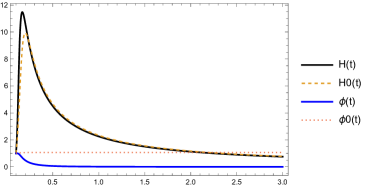
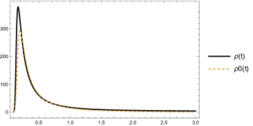
Figure 20: Numerical solutions $H(t)$, $\phi(t)$ and $\rho$ vs the asymptotic expansions $H_{0}(t)$, $\phi_{0}(t)$ and $\rho_{0}(t)$ defined respectively by (234), (237) and (236) (valid for $\xi=0$) for the initial conditions $\rho_{m}(0.1)=1,H(0.1)=1,\dot{\phi}(0.1)=1,\phi(0.1)=1$ and the parameter values $c_{1}=9.571429\times{10}^{-7}$, $c_{3}=7\times{10}^{-6}$, $c_{4}=-1.5$, $c_{5}=0.881801$, $\mu=1.1,\xi=\frac{1}{6},V(\phi)=\Lambda=1$ for $\varepsilon=0.1$. The accuracy of the asymptotic approximation is illustrated when $\varepsilon\rightarrow 0$ even though the analytical solutions are calculated for $\xi=0$.

In Figure 20, $H(t)$, $\phi(t)$ and $\rho$ are presented vs the asymptotic expansions $H_{0}(t)$, $\phi_{0}(t)$ and $\rho_{0}$ defined respectively by (234), (237) and (236) for the initial conditions $\rho_{m}(0.1)=1,H(0.1)=1,\dot{\phi}(0.1)=1,\phi(0.1)=1$ (arbitrarily chosen) and the parameter values $c_{1}=9.571429\times{10}^{-7}$, $c_{3}=7\times{10}^{-6}$, $c_{4}=-1.5$, $c_{5}=0.881801$, $\mu=1.1,\xi=\frac{1}{6},V(\phi)=\Lambda=1$ for $\varepsilon=0.1$. The accuracy of the asymptotic approximation when $\varepsilon\rightarrow 0$ is illustrated.

III.4.2 Asymptotic expansions for $\xi\to 0$

We consider the following expansions

$$\rho=\rho_{0}+\xi\rho_{1}+\mathcal{O}(\xi^{2}),\;H=H_{0}+\xi H_{1}+\mathcal{O}(\xi^{2}),\;\phi=\phi_{0}+\xi\phi_{1}+\mathcal{O}(\xi^{2}),$$

where we assume that the non-minimal coupling parameter is a perturbation parameter $0<\xi\ll 1$.

Replacing them in (147), (148) and (149) we have

$$-\frac{1}{t^{3}}\Big{[}-3t^{3}H_{0}\dot{\phi_{0}}^{2}+18t^{3}H_{0}^{3}+3\mu t^{2}H_{0}^{2}-39t^{2}H_{0}^{2}-3(\mu-1)(4\mu-11)tH_{0}$$

$$+3(\mu-2)(\mu-1)^{2}+t^{3}\dot{\rho_{0}}+\mu t^{2}\dot{\phi_{0}}^{2}-t^{2}\dot{\phi_{0}}^{2}\Big{]}$$

$$-\frac{\xi}{t^{3}}\Big{[}54t^{3}H_{0}^{2}H_{1}+6(\mu-13)^{2}H_{0}H_{1}-6t^{3}H_{0}\dot{\phi_{0}}\dot{\phi_{1}}+18t^{3}H_{0}\dot{\phi_{0}}^{2}$$

$$-18t^{3}H_{0}^{3}\phi_{0}^{2}-3t^{2}H_{0}^{2}\phi_{0}\left((\mu-13)\phi_{0}+12t\dot{\phi_{0}}\right)$$

$$-6t^{2}H_{0}\phi_{0}\left((\mu-1)\dot{\phi_{0}}+3tV^{\prime}(\phi_{0})\right)$$

$$+3(\mu-1)(4\mu-11)tH_{0}\phi_{0}^{2}-3tH_{1}\left((\mu-1)(4\mu-11)+t^{2}\dot{\phi_{0}}^{2}\right)$$

$$+t^{3}\dot{\rho_{1}}+2(\mu-1)t^{2}\dot{\phi_{0}}\dot{\phi_{1}}-6\mu t^{2}\dot{\phi_{0}}^{2}+6\mu\phi_{0}V^{\prime}(\phi_{0})$$

$$-6t^{2}\phi_{0}V(\phi_{0})+6t^{2}\dot{\phi_{0}}^{2}-3\mu^{3}\phi_{0}^{2}+6\mu^{2}t\phi_{0}\dot{\phi_{0}}+12\mu^{2}\phi_{0}^{2}$$

$$-12\mu t\phi_{0}\dot{\phi_{0}}-15\mu\phi_{0}^{2}+6t\phi_{0}\dot{\phi_{0}}+6\phi_{0}^{2}\Big{]}=0,$$ (240)

$$\frac{1}{t^{2}}\Big{[}-t^{2}\dot{H_{0}}-3t^{2}H_{0}^{2}-2\mu tH_{0}+8tH_{0}+(\mu-2)(\mu-1)\Big{]}$$

$$+\frac{\xi}{t^{2}}\Big{[}-6t^{2}H_{0}H_{1}+2t^{2}H_{0}\phi_{0}\dot{\phi_{0}}$$

$$-t^{2}\dot{H_{1}}-2(\mu-4)tH_{1}+2t^{2}\phi_{0}V^{\prime}(\phi_{0})-2t^{2}\dot{\phi_{0}}^{2}+2(\mu-1)t\phi_{0}\dot{\phi_{0}}\Big{]}=0,$$ (241)

$$-\frac{1}{t^{2}}\Big{[}3t^{2}H_{0}\dot{\phi_{0}}+t^{2}V^{\prime}(\phi_{0})+t^{2}\ddot{\phi_{0}}-\mu t\dot{\phi_{0}}+t\dot{\phi_{0}}\Big{]}$$

$$-\frac{\xi}{t^{2}}\Big{[}3t^{2}H_{0}\dot{\phi_{1}}+6\phi_{0}((\mu-2)(\mu-1)-tH_{0}(tH_{0}+2\mu-8))$$

$$+3t^{2}H_{1}\dot{\phi_{0}}+t^{2}\phi_{1}V^{\prime\prime}(\phi_{0})+t^{2}\ddot{\phi_{1}}-\mu t\dot{\phi_{1}}+t\dot{\phi_{1}}\Big{]}=0.$$ (242)

Assuming a constant potential $V(\phi)=\Lambda$, the zeroth and first-order equations are:

Zero order, $\mathcal{O}(\xi^{0})$:

$$\dot{\rho_{0}}=-\frac{(-3tH_{0}+\mu-1)\left(t\left(t\dot{\phi_{0}}^{2}-3H_{0}(2tH_{0}+\mu-5)\right)+3(\mu-2)(\mu-1)\right)}{t^{3}},$$ (243)

$$\dot{H_{0}}=\frac{tH_{0}(-3tH_{0}-2\mu+8)+(\mu-2)(\mu-1)}{t^{2}},$$ (244)

$$\ddot{\phi_{0}}=\frac{(-3tH_{0}+\mu-1)\dot{\phi_{0}}}{t},$$ (245)

with the constraint to order zero

$$-\frac{(\mu-1)H_{0}}{t}+H_{0}^{2}+\frac{1}{6}\left(-2(\Lambda+\rho_{0})-\dot{\phi_{0}}^{2}\right)=0.$$ (246)

The last two equations have the general solution

$$H_{0}(t)=\frac{-2\mu-\frac{2c_{1}rt_{0}^{r}}{t^{r}+c_{1}t_{0}^{r}}+r+9}{6t},$$ (247)

$$\phi_{0}(t)=\frac{2c_{2}\left(\frac{t}{t_{0}}\right)^{\frac{1}{2}(4\mu+r-9)}\,_{2}F_{1}\left(1,\frac{r+4\mu-9}{2r};\frac{3r+4\mu-9}{2r};-\frac{\left(\frac{t}{t_{0}}\right)^{r}}{c_{1}}\right)}{c_{1}(4\mu+r-9)}+\phi_{c},$$ (248)

where $c_{1}$, $c_{2}$ and $\phi_{c}$ are integration constants. Therefore, the first equation reduces to

$$\dot{\rho_{0}}= -\frac{\left(2\mu+r\left(-\frac{1}{2}+\frac{c_{1}t_{0}^{r}}{t^{r}+c_{1}t_{0}^{r}}\right)-\frac{11}{2}\right)}{6t^{3}}$$

$$\times\Bigg{(}20\mu^{2}-75\mu-\frac{r^{2}\left(t^{r}-c_{1}t_{0}^{r}\right){}^{2}}{\left(t^{r}+c_{1}t_{0}^{r}\right){}^{2}}+\frac{(\mu-3)r\left(t^{r}-c_{1}t_{0}^{r}\right)}{t^{r}+c_{1}t_{0}^{r}}+\frac{6c_{2}{}^{2}t^{4\mu+r-9}t_{0}^{-4\mu+r+9}}{\left(t^{r}+c_{1}t_{0}^{r}\right){}^{2}}+90\Bigg{)},$$ (249)

which is integrable, giving us the solution

$$\rho_{0}(t)= \frac{r^{3}}{24t^{2}}+\frac{r^{2}\left(-5\mu-\frac{8c_{1}t^{r}t_{0}^{r}}{\left(t^{r}+c_{1}t_{0}^{r}\right){}^{2}}+14\right)}{24t^{2}}-\frac{c_{2}{}^{2}t^{4\mu+r-11}t_{0}^{-4\mu+r+9}}{2\left(t^{r}+c_{1}t_{0}^{r}\right){}^{2}}$$

$$-\frac{r\left(16\mu^{2}-92\mu+\frac{8(5\mu-12)t^{r}}{t^{r}+c_{1}t_{0}^{r}}+153\right)}{24t^{2}}+\frac{5(4\mu-11)(\mu(4\mu-15)+18)}{24t^{2}}-\Lambda.$$ (250)

where $c_{3}=-\Lambda$ is an integration constant.

First order, $\mathcal{O}(\xi)$:

$$\dot{\rho_{1}}=\frac{1}{t^{3}}\Bigg{[}3tH_{1}\left(t\left(t\dot{\phi_{0}}^{2}-2H_{0}(9tH_{0}(t)+\mu-13)\right)+(\mu-1)(4\mu-11)\right)$$

$$+(-3tH_{0}+\mu-1)\Big{(}-6t\phi_{0}(2tH_{0}+\mu-1)\dot{\phi_{0}}$$

$$+3\phi_{0}^{2}((\mu-2)(\mu-1)-tH_{0}(2tH_{0}+\mu-5))+2t^{2}\dot{\phi_{0}}\left(3\dot{\phi_{0}}-\dot{\phi_{1}}\right)\Big{)}\Bigg{]},$$ (251)

$$\dot{H_{1}}=-\frac{2\left(H_{1}(3tH_{0}+\mu-4)-\phi_{0}(tH_{0}+\mu-1)\dot{\phi_{0}}+t\dot{\phi_{0}}^{2}\right)}{t},$$ (252)

$$\ddot{\phi_{1}}=-\frac{t\left((3tH_{0}-\mu+1)\dot{\phi_{1}}+3tH_{1}\dot{\phi_{0}}\right)+6\phi_{0}((\mu-2)(\mu-1)-tH_{0}(tH_{0}+2\mu-8))}{t^{2}},$$ (253)

with the restriction in the first order

$$\rho_{1}=\frac{H_{1}(6tH_{0}-3\mu+3)-3H_{0}\dot{\phi_{0}}\left(\phi_{0}(tH_{0}-\mu+1)+2t\dot{\phi_{0}}\right)-t\dot{\phi_{0}}\dot{\phi_{1}}}{t}.$$ (254)

This expression can be used to define $\rho_{1}$ such that the equation (251) is a compatibility condition that is satisfied for all $t$. Hence, we have a reduced system

$$\ddot{\phi_{1}}= -\frac{6c_{2}H_{1}t^{\frac{1}{2}(4\mu+r-9)}t_{0}^{\frac{1}{2}(-4\mu+r+9)}+\dot{\phi_{1}}\left((-4\mu+r+11)t^{r}-c_{1}(4\mu+r-11)t_{0}^{r}\right)}{2t\left(t^{r}+c_{1}t_{0}^{r}\right)}$$

$$+\frac{c_{2}t^{\frac{1}{2}(4\mu+r-9)-2}t_{0}^{-2\mu-\frac{r}{2}}\,{}_{2}F_{1}\left(1,\frac{r+4\mu-9}{2r};\frac{3r+4\mu-9}{2r};-\frac{t^{r}t_{0}^{-r}}{c_{1}}\right)}{3c_{1}(4\mu+r-9)\left(t^{r}+c_{1}t_{0}^{r}\right){}^{2}}$$

$$\times\Bigg{(}t_{0}^{9/2}\left(4(69-14\mu)\mu+r^{2}+(8\mu-30)r-423\right)t^{2r}$$

$$-2c_{1}\left(4\mu(14\mu-69)+r^{2}+423\right)t^{r}t_{0}^{r+\frac{9}{2}}+c_{1}{}^{2}\left(4(69-14\mu)\mu+r^{2}+(30-8\mu)r-423\right)t_{0}^{2r+\frac{9}{2}}\Bigg{)}$$

$$+\frac{\Lambda t_{0}^{2}\left(56\mu^{2}-276\mu-\frac{4r^{2}t^{2r}}{\left(t^{r}+c_{1}t_{0}^{r}\right){}^{2}}-r^{2}+8\mu r+\frac{4r(-4\mu+r+15)t^{r}}{t^{r}+c_{1}t_{0}^{r}}-30r+423\right)}{6t^{2}},$$ (255)

$$\dot{H_{1}} =\frac{H_{1}\left(-1+r\left(-1+\frac{2c_{1}t_{0}^{r}}{t^{r}+c_{1}t_{0}^{r}}\right)\right)}{t}$$

$$+\frac{2c_{2}{}^{2}t_{0}^{9-4\mu}t^{4\mu+r-11}\left((4\mu+r+3)t^{r}-c_{1}(-4\mu+r-3)t_{0}^{r}\right)\,_{2}F_{1}\left(1,\frac{r+4\mu-9}{2r};\frac{3r+4\mu-9}{2r};-\frac{t^{r}t_{0}^{-r}}{c_{1}}\right)}{3c_{1}(4\mu+r-9)\left(t^{r}+c_{1}t_{0}^{r}\right){}^{2}}$$

$$-\frac{c_{2}\Lambda t^{\frac{1}{2}(4\mu+r)-\frac{13}{2}}t_{0}^{\frac{1}{2}(-4\mu+r+13)}\left((4\mu+r+3)t^{r}-c_{1}(-4\mu+r-3)t_{0}^{r}\right)}{3\left(t^{r}+c_{1}t_{0}^{r}\right){}^{2}}-\frac{2c_{2}{}^{2}t^{4\mu+r-11}t_{0}^{-4\mu+r+9}}{\left(t^{r}+c_{1}t_{0}^{r}\right){}^{2}}.$$ (256)

The second equation is integrable, giving us

$$H_{1}(t)= -\frac{c_{2}{}^{2}(-4\mu+r-3)(4\mu+r-9)\Gamma\left(\frac{4\mu-9}{r}\right)t^{4\mu+r-10}t_{0}^{-4\mu-r+9}\,{}_{2}\tilde{F}_{1}\left(1,\frac{4\mu-9}{r};\frac{r+4\mu-9}{r};-\frac{\left(\frac{t}{t_{0}}\right)^{r}}{c_{1}}\right)}{36r\left(\left(\frac{t}{t_{0}}\right)^{r}+c_{1}\right){}^{2}}$$

$$-\frac{c_{2}{}^{2}(-4\mu+r+11)\Gamma\left(\frac{r+4\mu-9}{r}\right)t^{2(2\mu+r)-10}t_{0}^{-4\mu-2r+9}\,{}_{2}\tilde{F}_{1}\left(1,\frac{r+4\mu-9}{r};\frac{2r+4\mu-9}{r};-\frac{\left(\frac{t}{t_{0}}\right)^{r}}{c_{1}}\right)}{3c_{1}r\left(\left(\frac{t}{t_{0}}\right)^{r}+c_{1}\right){}^{2}}$$

$$+\frac{c_{2}t^{\frac{1}{2}(4\mu+r)-10}t_{0}^{-2(2\mu+r)}}{36\left(\left(\frac{t}{t_{0}}\right)^{r}+c_{1}\right){}^{2}}\Bigg{[}\frac{2c_{2}t_{0}^{9}t^{\frac{1}{2}(4\mu+r)}\left(12(-4\mu+r+11)t^{r}+c_{1}(-4\mu+r-3)(4\mu+r-9)t_{0}^{r}\right)}{c_{1}(4\mu+r-9)}$$

$$\times\,_{2}F_{1}\left(1,\frac{r+4\mu-9}{2r};\frac{3r+4\mu-9}{2r};-\frac{\left(\frac{t}{t_{0}}\right)^{r}}{c_{1}}\right)$$

$$-12\Lambda(-4\mu+r+11)t^{r+\frac{9}{2}}t_{0}^{\frac{1}{2}(4\mu+r+13)}+12c_{1}\Lambda t^{9/2}(4\mu+r-11)t_{0}^{\frac{1}{2}(4\mu+3r+13)}+\frac{72c_{2}t_{0}^{r+9}t^{\frac{1}{2}(4\mu+r)}}{9-4\mu}\Bigg{]}$$

$$+c_{4}\left(1+\frac{\left(\frac{t}{t_{0}}\right)^{r}}{c_{1}}\right){}^{-\frac{r+1}{r}}\left(1+c_{1}\left(\frac{t_{0}}{t}\right)^{r}\right){}^{\frac{1}{r}-1},$$ (257)

where $c_{4}$ is a constant of integration. The equation for $\phi_{1}$ can be solved in quadratures:

$$\phi_{1}(t)= \int_{1}^{t}\;e^{\left(\int_{1}^{\mu_{3}}\left(\frac{\mu-1}{\mu_{1}}-3H_{0}(\mu_{1})\right)d\mu_{1}\right)}\times\Bigg{[}c_{5}+\int_{1}^{\mu_{3}}\frac{e^{\left(-\int_{1}^{\mu_{2}}\left(\frac{\mu-1}{\mu_{1}}-3H_{0}(\mu_{1})\right)d\mu_{1}\right)}}{\mu_{2}^{2}}\Bigg{(}-3H_{1}(\mu_{2})\dot{\phi_{0}}(\mu_{2})\mu_{2}^{2}$$

$$-6((\mu-2)(\mu-1)-H_{0}(\mu_{2})\mu_{2}(2\mu+H_{0}(\mu_{2})\mu_{2}-8))\phi_{0}(\mu_{2})\Bigg{)}d\mu_{2}\Bigg{]}d\mu_{3}+c_{6},$$ (258)

where $c_{5}$ and $c_{6}$ are integration constants and $H_{0}(\mu_{1})$ is calculated using (247), $\dot{\phi_{0}}(\mu_{2})$ is calculated by taking the derivative with respect to $t$ of (248) and $\phi_{0}(\mu_{2})$ is evaluated using (248). Finally, the expression for $H_{1}(\mu_{2})$ is (257).

IV Conclusions

In this paper, corrections to the Friedman and Klein-Gordon equations based on the formalism of fractional calculus using Caputo’s derivative were studied. Thus, we have presented fractional calculus as a viable and attractive option for applications to the theory of gravity. Based on the knowledge of the different uses that have already been given to fractional calculus in other areas of physics and engineering and that are shown in the paper, a didactic exposition of the main aspects of fractional calculus has been presented, showing the different approaches that exist and definitions of fractional derivative.

This paper analyzed the fractional theory in cosmological models with a scalar field with a coupling constant $\xi$. We qualitatively analyze the case $\xi=0$ and mainly the general case of $\xi\neq 0$. Using different formulations of dynamical systems, examine their equilibrium points and determine how the fractional term affects their stability—exposing the complex behaviour presented by specific equilibrium points in the systems’ phase space and numerical solutions for different values for $\xi$ and $\mu$. We use methods from perturbation theory to analyze the cosmological behaviour obtaining solutions through two asymptotic expansions proposed for the system functions around the parameters $\mu=1$ and $\xi=0$ in which the model has recovered standard cosmology and the theory with minimal coupling to gravity with an excellent approximation to the numerical solutions of the system.

In the paper’s introductory section I, we discussed the challenges of traditional calculations in modelling power law phenomena. We then presented the various applications of fractional calculus, highlighting its effectiveness in recent studies in cosmology. This makes it a viable option to explore gravity theory further. We also introduced the research questions, posed the fractional formulation of the gravity problem, and outlined the paper’s general and specific objectives. We then described the methodology used to develop the paper. Finally, we emphasized the scientific novelty of this research. Specifically, we mentioned that our analysis of cosmologies with a scalar field with conformal and non-minimal coupling to gravity in the fractional context seeks to generalize previous results in the framework of the fractional formulation of gravity, making it a novel contribution.

Section II summarizes the main results of fractional calculus, mentioning some approaches to possible fractional derivatives such as Grünwald–Letnikov, Riemann–Liouville and Caputo. We review the known rules of differentiation in the fractional context under the different approaches and show the fractional derivative of known functions. Emphasis is placed on taking integration as an inverse operation of the differentiation to define fractional integration by generalizing Cauchy’s formula for iterated integrals, allowing us to define the fractional derivative. The Liouville, Riemann, Liouville-Caputo and Caputo derivatives were defined. Finally, we discussed what fractional differential equations are, using the tools of Wolfram Language 13.3 (Wolfram Research,, 2023), and we solved the classical problem of the harmonic oscillator and a physical problem of a point particle that moves under the effect of a friction force in the fractional context from different approaches.

It is important to emphasize that fractional differential equations, which involve fractional derivatives, generalize ordinary differential equations. Fractional differential equations have been widely used in engineering, physics, chemistry, biology and other fields involving relaxation and oscillation models, and very recently, they have been used in cosmology. For this reason, since the version of Wolfram Language 13.1, two basic operators for fractional calculation were implemented, the functions FractionalD and CaputoD. The algorithms of the MittagLefflerE functions have been updated, as they are of crucial importance in the theory of fractional calculus, and the powerful DSolve function was heavily updated in version 13.1 to support FDE. This paper solved several fractional differential equations using the DSolve function of Wolfram Language 13.3 (Wolfram Research,, 2023). The solutions to such equations are generally given in terms of the function MittagLefflerE, the primary function for fractional calculus applications. Its role in fractional differential equation solutions is similar in importance to the Exp function for ODE solutions: any ODE with constant coefficients can be solved in terms of Mittag-Leffler functions.

According to the analysis carried out in the paper, the behaviour of the fractional harmonic oscillator is very similar to the behaviour of the ordinary damped harmonic oscillator. These examples demonstrate that the order of a fractional differential equation can be used as a control parameter to model some complicated systems.

In section III, cosmological models were introduced within the fractional formulation of the gravity framework, and previous results were discussed where the coupling is minimal $\xi=0.$ The paper’s main result is the application of the tools defined in section II to fractional cosmologies with non-minimal coupling $\xi\neq 0.$ Different dynamical systems and relevant cases were studied, such as the invariant set $\Omega_{\Lambda}=0$. Some numerical integration methods from the specialized Mathematica software were used to study the behaviour of the solutions of the systems of differential equations coming from the cosmological model, and the stability of the critical points was studied using appropriate tools.

In the sections III.3.1 and III.4 we found a great technical difficulty when analyzing the stability of the curves and critical points $P_{6}(x_{c}):\left(x_{c},-\frac{1}{\sqrt{\xi}},\Omega_{\Lambda 0},0\right)$, $P_{7}(x_{c}):\left(x_{c},-\frac{1}{\sqrt{\xi}},0,0\right)$, $P_{8}:\left(0,-\frac{1}{\sqrt{\xi}},\Omega_{\Lambda 0},0\right)$, $P_{9}:\left(0,-\frac{1}{\sqrt{\xi}},0,0\right)$, $P_{10}(x_{c}):\left(x_{c},\frac{1}{\sqrt{\xi}},\Omega_{\Lambda 0},0\right)$, $P_{11}(x_{c}):\left(x_{c},\frac{1}{\sqrt{\xi}},0,0\right)$, $P_{12}:\left(0,\frac{1}{\sqrt{\xi}},\Omega_{\Lambda 0},0\right)$, $P_{13}:\left(0,\frac{1}{\sqrt{\xi}},0,0\right)$. Due to the complexity of the stability analysis of these sets of equilibrium points, numerical solution methods have to be used. However, partial stability information can be obtained by computing the eigenvalues using the time variable $\tau=\ln(a/a_{0})$ and taking the limit when $\alpha\rightarrow 0$.

In the study of curves $\left(0,-\frac{1}{\sqrt{\xi(12\xi+1)}},\Omega_{\Lambda 0},-\mu\mp\sqrt{\mu(2\mu-11)+18}+4\right)$ and
$\left(0,\frac{1}{\sqrt{\xi(12\xi+1)}},\Omega_{\Lambda 0},-\mu\mp\sqrt{\mu(2\mu-11)+18}+4\right)$ The technical difficulties lie in the parameter of the equation for the state of matter, which is complex and infinite. Furthermore, stability has to be determined numerically since the Jacobian matrix has infinite entries. These situations are due to the non-differentiability of the flow when $\alpha\rightarrow 0$ and $G:=(\xi(12\xi+1)y^{2}-1)\rightarrow 0.$ The last case is even more complex since in a neighbourhood of $G\equiv 0$, the direction of the flow changes, and they enter the context of non-smooth mechanics. In all these cases, the stability analysis of these curves/sets will be left for future research since they cannot be implemented with the techniques developed in this paper.

Non-smooth mechanics is a modelling approach that does not require the temporal evolutions of positions and velocities to be smooth functions. Due to possible impacts, the speeds of the mechanical system may jump at certain moments to comply with kinematic restrictions. Consider, for example, a rigid model of a ball falling to the ground. Just before the impact between the ball and the ground, the ball has a pre-impact velocity that does not disappear. At the instant of impact, the velocity must jump to a post-impact velocity of at least zero, or penetration will occur. Non-smooth mechanical models are often used in contact dynamics.

A review of research on non-smooth dynamical systems from the point of view of applications is provided in reference (Popp,, 2000). Two types of lack of smoothness are considered: impact and friction. A list of basic models is provided for each type, application areas are specified, and research results are reviewed. The literature on non-smooth dynamical systems will be reviewed in future work to resolve the difficulties above.

The research hypotheses were implemented during this research, and the paper’s general and specific objectives were satisfactorily addressed. It was possible to obtain relevant information on the flow properties associated with several autonomous systems of ordinary differential equations from the cosmological context through qualitative techniques from the dynamical systems theory. The review of the literature on dynamical systems and fractional calculus was exhaustive. The work tools used in the paper were appropriately selected, identifying the use of the Caputo fractional derivative and its application in formulating a fractional cosmological action and its respective variational calculation. The main results of fractional calculus for the qualitative analysis of cosmological models were presented in a didactic manner.

The analysis of cosmologies with a scalar field with conformal and non-minimal coupling to gravity in the fractional context is novel, generalizing previous results within the framework of the fractional formulation of gravity. From the mathematical point of view, it described the phase space of the models, obtaining qualitative results and explicit and approximated exact solutions with high numerical precision. That represents a different and attractive scenario due to its high level of applicability to describe natural phenomena.

Author contributions

Conceptualization, K.M., A.D.M. and G.L.; methodology, G.L.; software, K.M., A.D.M. and G.L.; validation, K.M., A.D.M. and G.L.; formal analysis, K.M., A.D.M., G.L., C.M. and A.P.; investigation, K.M., A.D.M., G.L., C.M. and A.P.; resources, G.L., C.M. and A.P.; writing—original draft preparation, G.L.; writing—review and editing, G.L., C.M. and A.P.; visualization, K.M., A.D.M. and G.L.; supervision, G.L. and A.M.; project administration, G.L. and K.M.; funding acquisition, K.M., A.D.M., G.L., C.M. and A.P. All authors have read and agreed to the published version of the manuscript.

Funding

K.M. and G.L. were funded by Vicerrectoría de Investigación y Desarrollo Tecnológico (VRIDT) at Universidad Católica del Norte (UCN) through Concurso Fondo de Tesis 2023 UCN, Resolución VRIDT N°063/2023. VRIDT-UCN funded G. L. through Resolución VRIDT No. 026/2023 and Resolución VRIDT No. 027/2023. G. L. also acknowledge the financial support of Proyecto de Investigación Pro Fondecyt Regular 2023, Resolución VRIDT No. 076/2023. A.D.M. was supported by Agencia Nacional de Investigación y Desarrollo - ANID Subdirección de Capital Humano/Doctorado Nacional/año 2020 folio 21200837, Gastos operacionales proyecto de tesis/2022 folio 242220121, and VRIDT-UCN. C. M. was supported by ANID Subdirección de Capital Humano/Doctorado Nacional/año 2021- folio 21211604. A.P. acknowledges the funding of VRIDT-UCN through Resolución VRIDT No. 096/2022 and Resolución VRIDT No. 098/2022.

Data availability

No new data were created or analyzed in this study. Data sharing is not applicable to this article.

Conflicts of interest

We declare no conflict of interest. The funders had no role in the design of the study; in the collection, analyses, or interpretation of data; in the writing of the manuscript; or in the decision to publish the results.

Appendix A Special functions

This appendix presents several special functions that appear recurrently in these topics.

A.1 Gamma Function

The Gamma function extends the factorial function; that is, it extends a function of integers to a function of real or complex numbers. Namely, for natural numbers, the factorial of $n$ is defined as

$$n!=1\times 2\times 3\times\cdots\times n=\prod_{j=1}^{n}j.$$ (259)

On the other hand, the Gamma function can be written as

$$\Gamma(z)=\int_{0}^{\infty}t^{z-1}e^{-t}\,dt,$$ (260)

which works for values of the complex number $z$ with $\Re(z)>0$. It can be observed that

$$\Gamma(z+1)=z\Gamma(z),$$ (261)

and also

$$\Gamma(n+1)=n!.$$ (262)

Additionally, one can write the binomial coefficient in terms of the Gamma function as

$$\begin{pmatrix}z\\ v\end{pmatrix}=\frac{z!}{v!(z-v)!}=\frac{\Gamma(z+1)}{\Gamma(v+1)\Gamma(z+1-v)}.$$ (263)

That added to the reflection formula,

$$\Gamma(z)\Gamma(1-z)=\frac{\pi}{\sin{(\pi z})},$$ (264)

and to the Incomplete Gamma function,

$$\Gamma(a,z)=\int_{z}^{\infty}t^{a-1}e^{-t}dt,$$ (265)

where

$$\Gamma(a,0)=\Gamma(a).$$ (266)

A.2 Mittag-Leffler functions

From the Maclaurin series expansion of the exponential,

$$e^{z}=\sum_{n=0}^{\infty}\frac{z^{n}}{n!},$$ (267)

We can replace the factorial with the Gamma function:

$$e^{z}=\sum_{n=0}^{\infty}\frac{z^{n}}{\Gamma(n+1)}.$$ (268)

That can then be extended as follows:

$$E(\alpha,z)=\sum_{n=0}^{\infty}\frac{z^{n}}{\Gamma(\alpha n+1)},$$ (269)

where $\alpha$ is an arbitrary real number greater than zero.

In fractional calculus, this function has a similar importance to that of the exponential function in standard calculus. For some values of $\alpha$ and functions of $z$, already known functions can be obtained:

$$E(2,-z^{2})=\cos{z},\hskip 20.075ptE(1/2,z^{1/2})=e^{z}\left[1+\text{erf}(z^{1/2})\right],$$ (270)

where the Error function, $\text{erf}(z)$, is given by

$$\text{erf}(z)=\frac{2}{\sqrt{\pi}}\int_{0}^{z}e^{-t^{2}}dt.$$ (271)

The Mittag-Leffler function can also be extended as follows:

$$E(\alpha,\beta,z)=\sum_{n=0}^{\infty}\frac{z^{n}}{\Gamma(\alpha n+\beta)},$$ (272)

which is known as the generalized Mittag-Leffler function and has several special cases, e.g.

$$E(1,2,z)=\frac{e^{z}-1}{z},\hskip 20.075ptE(2,2,z^{2})=\frac{\sinh{(z)}}{z}.$$ (273)

A.3 Hypergeometric functions

These functions contain many particular cases of special functions and are widely used in fractional calculus. From the definition

$${}_{p}{F_{q}}(\{a_{i}\};\{b_{j}\};z)=\frac{\prod_{j=1}^{q}\Gamma(b_{j})}{\prod_{i=1}^{p}\Gamma(a_{i})}\sum_{n=0}^{\infty}\frac{\prod_{i=1}^{p}\Gamma(a_{i}+n)z^{n}}{\prod_{j=1}^{q}\Gamma(b_{j}+n)n!},$$ (274)

It follows that the derivative with respect to $z$ is

$$\frac{d}{dz}\left[{}_{p}{F_{q}}(\{a_{i}\};\{b_{j}\};z)\right]=\frac{\prod_{i=1}^{p}\Gamma(a_{i})}{\prod_{j=1}^{q}\Gamma(b_{j})}\left[{}_{p}{F_{q}}(\{a_{i}+1\},\{b_{j}+1\};z)\right].$$ (275)

References

- West, (2021) West, B.J. (2021) Fractional Calculus and the Future of Science. Entropy 2021, 23, 1566.
- (2) Calcagni, G. (2010a). Fractal universe and quantum gravity. Phys. Rev. Lett., 104:251301.
- (3) Calcagni, G. (2010b). Quantum field theory, gravity and cosmology in a fractal universe. JHEP, 03:120.
- Jalalzadeh et al., (2021) Jalalzadeh, S., da Silva, F. R., and Moniz, P. V. (2021). Prospecting black hole thermodynamics with fractional quantum mechanics. Eur. Phys. J. C, 81 (7):632.
- Lim, (2006) Lim, S. C. (2006). fractional derivative quantum fields at positive temperature. Physica A, 363:269–281.
- Lim and Eab, (2019) Lim, S. C. and Eab, C. H. (2019). Fractional quantum fields, pages 237–256. De Gruyter.
- Moniz and Jalalzadeh, (2020) Moniz, P. V. and Jalalzadeh, S. (2020). From Fractional Quantum Mechanics to Quantum Cosmology: An Overture. Mathematics, 8 (3):313.
- Rasouli et al., (2021) Rasouli, S. M. M., Jalalzadeh, S., and Moniz, P. V. (2021). Broadening quantum cosmology with a fractional whirl. Mod. Phys. Lett. A, 36 (14):2140005.
- V. Moniz and Jalalzadeh, (2020) V. Moniz, P. and Jalalzadeh, S. (2020). Challenging Routes in Quantum Cosmology. World Scientific Publishing, Singapore.
- El-Nabulsi, (2009) El-Nabulsi, R. A. (2009) Fractional Lagrangian Formulation of General Relativity and Emergence of Complex, Spinorial and Noncommutative Gravity. Int. J. Geom. Methods Mod. Phys. 2009, 6, 25–76.
- El-Nabulsi, (2010) El-Nabulsi, R. A. (2010) Modifications at Large Distances From Fractional and Fractal Arguments. Fractals 2010, 18, 185–190. https://doi.org/10.1142/S0218348X10004828.
- El-Nabulsi, (2011) El-Nabulsi, A.R. (2011) The fractional white dwarf hydrodynamical nonlinear differential equation and emergence of quark stars. Appl. Math. Comput. 2011, 218, 2837–2849.
- El-Nabulsi, (2012) El-Nabulsi, R. A. (2012) Glaeske-Kilbas-Saigo fractional integration and fractional Dixmier trace. Acta Math. Vietnam. 2012, 37, 149–160.
- (14) El-Nabulsi, R. A. (2013a) fractional derivatives generalization of Einstein‘s field equations. Indian J. Phys. 2013, 87, 195–200. https://doi.org/10.1007/s12648-012-0201-4.
- El-Nabulsi, (2015) El-Nabulsi, R. A. (2015) Fractional elliptic operator of order 2/3 from Glaeske-Kilbas-Saigo fractional integral transform. Funct. Anal. Approx. Comput 2015, 7, 29–33.
- (16) El-Nabulsi, R. A. (2016a). A Cosmology Governed by a Fractional Differential Equation and the Generalized Kilbas-Saigo-Mittag-Leffler Function. Int. J. Theor. Phys., 55 (2):625–635.
- El-Nabulsi, (2018) El-Nabulsi, R. A. (2018) Finite two-point space without quantization on noncommutative space from a generalized fractional integral operator. Complex Anal. Oper. Theory 2018, 12, 1609–1616.
- El-Nabulsi, (2020) El-Nabulsi, R. A. (2020) On generalized fractional spin, fractional angular momentum, fractional momentum operators in quantum mechanics. Few-Body Syst. 2020, 61, 25.
- El-Nabulsi and Wu, (2012) El-Nabulsi, R. A. ; Wu, C.G. (2012) Fractional Complexified Field Theory from Saxena-Kumbhat Fractional Integral, fractional derivative of Order () and Dynamical Fractional Integral Exponent. Afr. Diaspora J. Math. New Ser. 2012, 13, 45–61.
- Rami, (2009) Rami, E.N.A. (2009) Fractional dynamics, fractional weak bosons masses and physics beyond the standard model. Chaos Solitons Fractals 2009, 41, 2262–2270.
- Wolfram Research, (2023) Wolfram Research, I. (2023) Mathematica, Version 13.3. Champaign, IL, 2023.
- Bandyopadhyay and Kamal, (2014) Bandyopadhyay, B. and Kamal, S. (2014). Stabilization and Control of Fractional Order Systems: A Sliding Mode Approach. Lecture Notes in Electrical Engineering. Springer International Publishing.
- Herrmann, (2014) Herrmann, R. (2014). Fractional Calculus: An Introduction For Physicists (2nd Edition). World Scientific Publishing Company.
- Kilbas et al., (2006) Kilbas, A., Srivastava, H., and Trujillo, J. (2006). Theory and applications of fractional differential equations. North Holland Mathematical Studies, 204.
- Klafter et al., (2012) Klafter, J., Lim, S. C., and Metzler, R. (2012). Fractional Dynamics: Recent Advances. World Scientific.
- Lorenzo and Hartley, (2016) Lorenzo, C. F. and Hartley, T. T. (2016). The Fractional Trigonometry: With Applications to Fractional Differential Equations and Science. Wiley.
- Malinowska et al., (2015) Malinowska, A. B., Odzijewicz, T., and Torres, D. F. M. (2015). Advanced Methods in the Fractional Calculus of Variations. Springer briefs in applied sciences and technology. Springer International Publishing.
- Monje et al., (2010) Monje, C. A., Chen, Y. Q., Vinagre, B. M., Xue, D., and Feliu-Batlle, V. (2010). Fractional-order Systems and Controls: Fundamentals and Applications. Advances in Industrial Control. Springer London.
- Padula and Visioli, (2014) Padula, F. and Visioli, A. (2014). Advances in Robust Fractional Control. Springer International Publishing.
- Podlubny, (1998) Podlubny, I. (1998). Fractional Differential Equations, Volume 198. Elsevier.
- Tarasov, (2013) Tarasov, V. E. (2013). Review of some promising fractional physical models. International Journal of Modern Physics B, 27 (9).
- Tarasov, (2019) Tarasov, V. E. (2019). Applications in Physics, Part A. De Gruyter Reference. De Gruyter.
- Uchaikin, (2013) Uchaikin, V. V. (2013). fractional derivatives for physicists and Engineers. Higher Education Press.
- Stanislavsky, (2004) Stanislavsky, A. (2004). Fractional oscillator. Phys. Rev. E 70, 051103.
- Agrawal, (2007) Agrawal, O, P. (2007). Fractional variational calculus in terms of Riesz fractional derivatives. Journal of Physics A: Mathematical and Theoretical, 2007, vol. 40, no 24, p. 6287.
- Baleanu and Muslih, (2005) Baleanu, D. and Muslih, S. (2005). Lagrangian formulation of classical fields within Riemann-Liouville fractional derivatives. In International Design Engineering Technical Conferences and Computers and Information in Engineering Conference (Vol. 47438, pp. 1457-1464).
- Baleanu and Trujillo, (2010) Baleanu, D. and Trujillo, J. (2010). A new method of finding the fractional Euler-Lagrange and Hamilton equations within caputo fractional derivatives. Communications in Nonlinear Science and Numerical Simulation, 2010, vol. 15, no 5, p. 1111-1115.
- El-Nabulsi and Torres, (2008) El-Nabulsi, R. A. and Torres, D, F. (2008). Fractional action-like variational problems Journal of Mathematical Physics, 2008, vol. 49, no 5.
- (39) Odzijewicz, T., Malinowska, A., and Torres, D. (2013a). Generalized fractional calculus with applications to the calculus of variations. Computers & Mathematics with Applications, 2012, vol. 64, no 10, p. 3351-3366.
- (40) Odzijewicz, T., Malinowska, A., and Torres, D. (2013b). Noether’s theorem for fractional variational problems of variable order. Open Physics, 2013, vol. 11, no 6, p. 691-701.
- (41) Odzijewicz, T., Malinowska, A., and Torres, D. (2013c). Variable order fractional variational calculus for double integrals. In 2012 IEEE 51st IEEE Conference on Decision and Control (CDC) (pp. 6873-6878). IEEE.
- Calcagni, (2013) Calcagni, G. (2013). Multi-scale gravity and cosmology. JCAP, 12:041.
- (43) Calcagni, G. (2017a). Complex dimensions and their observability. Phys. Rev. D, 96 (4):046001.
- (44) Calcagni, G. (2017b). Multifractional theories: an unconventional review. JHEP, 03:138. [Erratum: JHEP 06, 020 (2017)].
- (45) Calcagni, G. (2021a). Classical and quantum gravity with fractional operators. Class. Quant. Grav., 38 (16):165005. [Erratum: Class.Quant.Grav. 38, 169601 (2021)].
- (46) Calcagni, G. (2021b). Multifractional theories: an updated review. Mod. Phys. Lett. A, 36 (14):2140006.
- (47) Calcagni, G. (2021c). Quantum scalar field theories with fractional operators. Classical and Quantum Gravity, 38 (16):165006.
- Calcagni and De Felice, (2020) Calcagni, G. and De Felice, A. (2020). Dark energy in multifractional spacetimes. Phys. Rev. D, 102 (10):103529.
- Calcagni and Kuroyanagi, (2021) Calcagni, G. and Kuroyanagi, S. (2021). Stochastic gravitational-wave background in quantum gravity. JCAP, 03:019.
- Calcagni et al., (2019) Calcagni, G., Kuroyanagi, S., Marsat, S., Sakellariadou, M., Tamanini, N., and Tasinato, G. (2019). Quantum gravity and gravitational-wave astronomy. JCAP, 10:012.
- Calcagni et al., (2016) Calcagni, G., Kuroyanagi, S., and Tsujikawa, S. (2016). Cosmic microwave background and inflation in multi-fractional spacetimes. JCAP, 08:039.
- Debnath et al., (2012) Debnath, U., Jamil, M., and Chattopadhyay, S. (2012). Fractional Action Cosmology: Emergent, Logamediate, Intermediate, Power Law Scenarios of the Universe and Generalized Second Law of Thermodynamics. International Journal of Theoretical Physics, 51:812–837.
- Debnath et al., (2013) Debnath, U., Chattopadhyay, S., and Jamil, M. (2013). Fractional action cosmology: some dark energy models in emergent, logamediate, and intermediate scenarios of the universe. Journal of Theoretical and Applied Physics, 7:25.
- El-Nabulsi, (2012) El-Nabulsi, R. A. (2012). Gravitons in fractional action cosmology. Int. J. Theor. Phys., 51:3978–3992.
- (55) El-Nabulsi, R. A. (2013b). Non-minimal coupling in fractional action cosmology. Indian J. Phys., 87:835–840.
- (56) El-Nabulsi, R. A. (2013c). Nonstandard fractional exponential Lagrangians, fractional geodesic equation, complex general relativity, and discrete gravity. Can. J. Phys., 91 (8):618–622.
- (57) El-Nabulsi, R. A. (2016b). Implications of the Ornstein-Uhlenbeck-like fractional differential equation in cosmology. Rev. Mex. Fis., 62 (3):240.
- (58) El-Nabulsi, R. A. (2017a). Fractional Action Cosmology with Variable Order Parameter. Int. J. Theor. Phys., 56 (4):1159–1182.
- (59) El-Nabulsi, R. A. (2017c). Wormholes in fractional action cosmology. Can. J. Phys., 95 (6):605–609.
- García-Aspeitia et al., (2022) García-Aspeitia, M. A., Fernandez-Anaya, G., Hernández-Almada, A., Leon, G., and Magaña, J. (2022). Cosmology under the fractional calculus approach. Mon. Not. Roy. Astron. Soc., 517 (4):4813–4826.
- Giusti, (2020) Giusti, A. (2020). MOND-like Fractional Laplacian Theory. Phys. Rev. D, 101 (12):124029.
- Jalalzadeh et al., (2022) Jalalzadeh, S., Costa, E. W. O., and Moniz, P. V. (2022). de Sitter fractional quantum cosmology. Phys. Rev. D, 105 (12):L121901.
- Jamil et al., (2012) Jamil, M., Momeni, D., and Rashid, M. A. (2012). Fractional Action Cosmology with Power Law Weight Function. J. Phys. Conf. Ser., 354:012008.
- (64) Landim, R.G. Fractional dark energy: Phantom behavior and negative absolute temperature. Phys. Rev. D 2021, 104, 103508. https://doi.org/10.1103/PhysRevD.104.103508.
- (65) Landim, R.G. Fractional dark energy. Phys. Rev. D 2021, 103, 083511. https://doi.org/10.1103/PhysRevD.103.083511.
- Micolta-Riascos et al., (2023) Micolta-Riascos, B., Millano, A. D., Leon, G., Erices, C., and Paliathanasis, A. (2023). Revisiting fractional cosmology. Fractal and Fractional, 7 (2).
- Rami, (2015) Rami, E.-N. A. (2015). Fractional action oscillating phantom cosmology with conformal coupling. Eur. Phys. J. Plus, 130 (6):102.
- Roberts, (2014) Roberts, M. D. (2014). fractional derivative Cosmology. SOP Trans. Theor. Phys., 1:310.
- Shchigolev, (2011) Shchigolev, V. K. (2011). Cosmological Models with fractional derivatives and Fractional Action Functional. Commun. Theor. Phys., 56:389–396.
- (70) Shchigolev, V. K. (2013a). Cosmic Evolution in Fractional Action Cosmology. Discontinuity Nonlinearity and Complexity, 2 (2):115–123.
- (71) Shchigolev, V. K. (2013b). Fractional Einstein-Hilbert Action Cosmology. Mod. Phys. Lett. A, 28:1350056.
- Shchigolev, (2016) Shchigolev, V. K. (2016). Testing Fractional Action Cosmology. Eur. Phys. J. Plus, 131 (8):256.
- Shchigolev, (2021) Shchigolev, V. K. (2021). Fractional-order derivatives in cosmological models of accelerated expansion. Mod. Phys. Lett. A, 36 (14):2130014.
- Vacaru, (2010) Vacaru, S. I. (2010). New Classes of Off-Diagonal Cosmological Solutions in Einstein Gravity. Int. J. Theor. Phys., 49:2753–2776.
- (75) Vacaru, S. I. (2012a). Fractional Dynamics from Einstein Gravity, General Solutions, and Black Holes. Int. J. Theor. Phys., 51:1338–1359.
- (76) Vacaru, S. I. (2012b). Fractional Nonholonomic Ricci Flows. Chaos Solitons Fractals, 45:1266–1276.
- Hernández-Almada et al., (2020) Hernández-Almada, A., Leon, G., Magaña, J., García-Aspeitia, M. A., and Motta, V. (2020). Generalized Emergent Dark Energy: observational Hubble data constraints and stability analysis. Mon. Not. Roy. Astron. Soc., 497 (2):1590–1602.
- Hernández-Almada et al., (2022) Hernández-Almada, A., Leon, G., Magaña, J., García-Aspeitia, M. A., Motta, V., Saridakis, E. N., and Yesmakhanova, K. (2022). Kaniadakis-holographic dark energy: observational constraints and global dynamics. Mon. Not. Roy. Astron. Soc., 511 (3):4147–4158.
- Hernández-Almada et al., (2021) Hernández-Almada, A., Leon, G., Magaña, J., García-Aspeitia, M. A., Motta, V., Saridakis, E. N., Yesmakhanova, K., and Millano, A. D. (2021). Observational constraints and dynamical analysis of Kaniadakis horizon-entropy cosmology. Mon. Not. Roy. Astron. Soc., 512(4), 5122-5134.
- Leon et al., (2021) Leon, G., Magaña, J., Hernández-Almada, A., García-Aspeitia, M. A., Verdugo, T., and Motta, V. (2021). Barrow Entropy Cosmology: an observational approach with a hint of stability analysis. JCAP, 12 (12):032.
- González et al., (2023) González, E., Leon, G., and Fernandez-Anaya, G. (2023). Exact solutions and cosmological constraints in fractional cosmology. Fractal Fract., 7:368.
- Leon Torres et al., (2023) Leon, G., García-Aspeitia, M. A. , Fernandez-Anaya,G. , Hernández-Almada, A. , Magaña, J. , and González, E. , Cosmology under the fractional calculus approach: a possible tension resolution?, PoS CORFU2022 (2023), 248 doi:10.22323/1.436.0248 [arXiv:2304.14465 [gr-qc]].
- Di Valentino et al., (2021) Di Valentino, E., Mena, O., Pan, S., Visinelli, L., Yang, W., Melchiorri, A., Mota, D. F., Riess, A. G., and Silk, J. (2021). In the realm of the Hubble tension—a review of solutions. Class. Quant. Grav., 38 (15):153001.
- Efstathiou, (2021) Efstathiou, G. (2021). To H0 or not to H0? Mon. Not. Roy. Astron. Soc., 505 (3):3866–3872.
- Barrientos et al., (2021) Barrientos, E., Mendoza, S., and Padilla, P. (2021). Extending Friedmann equations using fractional derivatives using a Last Step Modification technique: the case of a matter dominated accelerated expanding Universe. Symmetry, 13 (2):174.
- El-Nabulsi, (2005) El-Nabulsi, R. A. (2005). Fractional unstable Euclidean universe. Electron. J. Theor. Phys., 2 (8):1–11.
- (87) El-Nabulsi, R. A. (2007a). Accelerated universe dominated by holographic dark energy, supergravity inflationary potential. Rom. J. Phys., 52:163–170.
- (88) El-Nabulsi, R. A. (2007b). Cosmology with a fractional action principle. Rom. Rep. Phys., 59:763–771.
- El-Nabulsi, (2008) El-Nabulsi, R. A. (2008). Increasing effective gravitational constant in fractional ADD brane cosmology. Electron. J. Theor. Phys., 5 (17):0103–106.
- Frederico and Torres, (2008) Frederico, G. S. F. and Torres, D. F. M. (2008). Necessary optimality conditions for fractional action-like problems with intrinsic and observer times. WSEAS Trans. Math., 7:6–11.
- Aghanim et al., (2020) Aghanim, N. et al. (2020). Planck 2018 results. VI. Cosmological parameters. Astron. Astrophys., 641:A6. [Erratum: Astron.Astrophys. 652, C4 (2021)].
- Carroll et al., (2004) Carroll, S., Addison-Wesley (2004). Spacetime and Geometry: An Introduction to General Relativity. Addison Wesley.
- Carroll, (2019) Carroll, S. M. (2019). Spacetime and geometry. Cambridge University Press.
- Wald, (2010) Wald, R. M. (2010). General relativity. University of Chicago press, Chicago.
- Foreman-Mackey et al., (2013) Foreman-Mackey, D., Hogg, D. W., Lang, D., and Goodman, J. (2013). emcee: The MCMC hammer. Publications of the Astronomical Society of the Pacific, 125 (925):306–312.
- Tavakol, (1997) Tavakol, R. (1997). Introduction to dynamical systems, ch 4. Part one, pp. 84–98. Cambridge University Press.
- Wainwright and Ellis, (1997) Wainwright, J. and Ellis, G. F. R., editors (1997). Dynamical Systems in Cosmology. Cambridge Univ. Press.
- Perko, (2001) Perko, L. (2001). Differential equations and dynamical systems, third edition. Springer-Verlag.
- Coley, (2003) Coley, A. (2003). Dynamical systems and cosmology, volume 291. Kluwer, Dordrecht, Netherlands.
- Hirsch et al., (2004) Hirsch, M. W., Smale, S., and Devaney, R. (2004). Differential equations, dynamical systems, and an introduction to chaos. London: Academic Press, San Diego, CA.
- Wiggins, (2006) Wiggins, S. (2006). Introduction to Applied Nonlinear Dynamical Systems and Chaos. Texts in Applied Mathematics. Springer.
- Berglund and Gentz, (2006) Berglund, N., and B. Gentz, B., Noise-Induced Phenomena in Slow-Fast Dynamical Systems, Series: Probability and Applications, Springer-Verlag: London, (2006).
- Fenichel, (1979) Fenichel, N., (1979) Geometric singular perturbation theory for ordinary differential equations. Journal of Differential Equations 31, 53-98.
- Fusco and Hale, (1988) Fusco, G., and Hale, J.K., Journal of Dynamics and Differential Equations 1, 75 (1988).
- Dumortier and Roussarie, (1995) Dumortier, F., and Roussarie, R., (1995) Canard cycles and center manifolds, (Memoirs of the American Mathematical Society, 577).
- Holmes, (2013) Holmes, M. H., (2013) “Introduction to Perturbation Methods”, (Springer Science+Business Media New York, ISBN 978-1-4614-5477-9) https://doi.org/10.1007/978-1-4614-5477-9.
- Kevorkian, (1981) Kevorkian, J., Cole, J.D., (1981) “Perturbation Methods in Applied Mathematics” (Applied Mathematical Sciences Series, Volume 34, Springer-Verlag New York eBook ISBN 978-1-4757-4213-8 https://doi.org/10.1007/978-1-4612-3968-0.
- Verhulst, (2000) Verhulst, F., (2000) “Methods and Applications of Singular Perturbations: Boundary Layers and Multiple Timescale Dynamics” (Springer-Verlag New York, ISBN 978-0-387-22966-9) https://doi.org/10.1007/0-387-28313-7.
- Popp, (2000) Popp, K. (2000). Non-smooth mechanical systems. Journal of Applied Mathematics and Mechanics, 64 (5):765–772.