Coupled coherent states method for tunneling dynamics: an interpretative study

Abstract

Numerical solutions of the time-dependent Schrödinger equation based on the variational principle may offer physical insight that cannot be gained by a solution using fixed grids in position and momentum space. Here we focus on the tunneling dynamics in a quartic double-well and the use of classical, trajectory-guided coherent states to gain insight into the workings of the coupled coherent states method developed by Shalashilin and Child [J. Chem. Phys. 113, 10028 (2000)]. It is shown that over-the-barrier classical trajectories, alone, can accurately describe the tunneling effect.

1 Introduction

Since several decades, variational methods to solve the time-dependent Schrödinger equation (TDSE) have been used in the chemical physics community [1, 2, 3, 4], where they are employed to study the quantum dynamics of molecular systems with a considerable number of degrees of freedom. Although seminal work on the variational principle is also known in the theoretical physics community [5], related numerical approaches in the time-domain have seen widespread use only more recently, with the advent of matrix product state techniques [6, 7] for the study of entanglement in finite lattice dynamics.

In molecular physics, the use of Glauber coherent states [8] with time-dependent parameters is especially appealing, because (i) often the initial states are ground vibrational states of the ground electronic potential energy surface and thus of Gaussian nature and (ii) methods based on Gaussian basis functions allow to gain an understanding of the quantum dynamics by, e.g., restricting the center parameters to follow classical trajectories in phase space. An intriguing example is given by a study on the one-dimensional Morse oscillator model that has been done by Wang and Heller. By using the semiclassical Herman-Kluk (HK) propagator [9], these authors have shown that the quantal revival dynamics present in this system can be understood as a subtle interference phenomenon of classical trajectories that are spread “all over phase space” [10]. Whereas the HK propagator has also proven useful in the study of Bose-Hubbard dynamics for small well numbers [11, 12, 13], its use for the tunneling dynamics in a double well is not appropriate, if a single wavepacket calculation is desired [14]. We will therefore base our numerical investigations on the so-called coupled coherent states (CCS) method by Shalashilin and Child [15]. In this method, the coherent state parameters are still classical, like in the HK case, but the coefficients in the expansion of the wavefunction are determined variationally, in contrast to the HK case, where they again follow from the (linearized) classical dynamics, see [4] for a recent review.

The presentation is structured as follows: First in Section 2, we briefly review the Hamiltonian of the quartic double well. In Section 3 we then recapitulate the coupled coherent states method [15] and the modification of the classical Hamiltonian due to normal ordering. In Section 4 we present numerical results for the tunneling dynamics, using suitably tailored rectangular grids of initial conditions in phase space, that allow us to discriminate the power of low as well as of high energy classical trajectories to describe tunneling. A brief summary and outlook are given in the last section.

2 The quartic double-well model

We start the main body of the presentation with a brief review of the double-well potential in one dimension, which is a model well suited to study coherent tunneling dynamics. It has many applications, one of the most important ones being the ammonia molecule, first discussed with respect to the tunneling effect by Hund as early as 1927 [16]. A solid state realization is given by a suitably parametrized rf-SQUID, where the role of the coordinate is played by the flux through the ring [17]. More recently bistable potentials have been discussed in cold-atom physics in connection with Bose-Einstein condensation [18]. The effect of an external sinusoidal field on the tunneling is quite counterintuitive, as an appropriately chosen field can lead to a complete stand-still of the tunneling dynamics [19].

For a particle of unit mass, the quartic double-well oscillator is governed by a Hamilton operator of the form

$$H(\hat{p},\hat{q})=\frac{\hat{p}^{2}}{2}+V(\hat{q}),$$ (1)

with the potential function

$$V(q)=-\frac{a}{2}q^{2}+\frac{b}{4}q^{4}+E_{B},\qquad a,b\in\Re^{+}.$$ (2)

It has quadratic minima at $q_{\pm}=\pm\sqrt{\frac{a}{b}}$ and a quadratic maximum at $q_{0}=0$ of height $E_{B}=\frac{a^{2}}{4b}$. By demanding that the second derivative of the potential at the symmetric minima be unity and the barrier height be $D$, we fix the parameters to be $a=1/2$ and $b=1/(16D)$.

The phase space portrait of the dynamics contains the prototypical separatrix, defined by $H(p,q)=D$ and shaped like the number eight rotated by 90 degrees, as displayed in Fig. 1, as well as a hyperbolic fixed point at $p=0,q=0$ on that separatrix and two elliptic fixed points at $p=0,q=q_{\pm}$ [20]. In the figure, we also display the modification of the separatrix due to normal ordering, as explained in Sect. 3.

Figure 1: Separatrix in the phase space of the quartic double well with $D=1$ for the standard classical Hamiltonian (the larger “8”) and for its normal ordered version (the smaller “8”).

If the available energy is higher than the barrier, a classical particle starting on the right side of the barrier can reach the left one and get back in a periodic fashion.

Quantum mechanically, in the usual tunneling scenario, where a Gaussian is sitting at the minimum of one of the two wells initially, with average energy below the barrier, the particle is still moving to the other well and back with a (usually very small) frequency given by the difference $E_{2}-E_{1}$ of the two lowest eigenvalues of the Hamilton operator. This motion is also referred to as umbrella motion. The case of an initial state starting from the top of the barrier is referred to as toppling pencil motion and has been studied classically in detail by Dittrich and Pena Martínez [21] as well as quantum mechanically in [22], where the influence of a finite number of bath degrees of freedom on the central degree of freedom (the double well) has been investigated.

3 The method of coupled coherent states

The numerical method for the solution of the TDSE, to be used in the following, is the coupled coherent states method developed by Shalashilin and Child [15, 23]. It is most clearly formulated by using a complexified phase space variable, defined by

$$z(t)=\frac{\gamma^{1/2}q(t)+{\rm i}\hbar^{-1}\gamma^{-1/2}p(t)}{\sqrt{2}},$$ (3)

where $\gamma=m\omega/\hbar$. In the remainder of the presentation, we set $\hbar$ as well as $m$ equal to unity and use Gaussian basis functions, which correspond to the coherent states of a harmonic oscillator with oscillation frequency $\omega=1$ (in dimensionless units) and the definition above simplifies considerably.

In the coupled coherent states (CCS) method of Shalashilin and Child, an ansatz is made for the time-evolved wavefunction as a finite esum in the form

$$\Ket{\Psi(t)}=\sum_{l=1}^{M}a_{l}(t)\Ket{z_{l}(t)},$$ (4)

where each ket $\Ket{z_{l}(t)}$ is a coherent state (an eigenstate of the annihilation operator) with a time-dependent, complex center parameter $z_{l}(t)$ and the “multiplicity” of the ansatz is given by $M$. The set of the $M$ center parameters is following uncoupled classical trajectories, each of which is fulfilling [23]

$${\rm i}\partial_{t}z=\partial_{z^{\ast}}H_{\rm ord}(z^{\ast},z),$$ (5)

which are Hamilton’s equations in complex notation. The normal ordered Hamiltonian is gained by using

$$\hat{q}=\frac{1}{\sqrt{2}}(\hat{a}^{\dagger}+\hat{a}),\qquad\hat{p}={\rm i}{\frac{1}{\sqrt{2}}}(\hat{a}^{\dagger}-\hat{a}),$$ (6)

in Eq. (1), and moving all creation operators to the left, by using the fundamental commutation relation

$$[\hat{a},\hat{a}^{\dagger}]=\hat{1}.$$ (7)

Then we replace $\hat{a}^{\dagger}$ by $z^{\ast}$ and $\hat{a}$ by $z$ to arrive at the classical Hamiltonian [22]

$$H_{\rm ord} = -\frac{1}{4}\left[\left(z^{\ast}-z\right)^{2}-1\right]-\frac{1}{8}\left[\left(z^{\ast}+z\right)^{2}+1\right]$$ (8)

$$+\frac{1}{256D}\left[\left(z^{\ast}+z\right)^{4}+6\left(z^{\ast}+z\right)^{2}+3\right].$$

We stress that by expressing the $z$ variable again in terms of position and momentum and by gathering all constant terms in the potential, a modified, normal ordered version of the potential emerges (see also [14]), that is given by

$$V_{\rm ord}(q)=D-\frac{1}{4}\left(q^{2}-\frac{1}{2}\right)+\frac{1}{64D}\left(q^{4}+3q^{2}+\frac{3}{4}\right).$$ (9)

Its minima are slightly shifted to $q_{\pm}=\pm\sqrt{8D-3/2}$ and the relative maximum at $q=0$ is increased to $V_{\rm ord}(0)=D+1/8+3/(256D)$. Due to the fact that the value of the ordered potential at the mimima is now not zero any more but given by $V_{\rm ord}(q_{\pm})=1/2-6/(256D)$, the barrier height is changed (typically decreased) to $D-3/8+9/(256D)$. These changes also lead to a change of the separatrix, which is highlighted in Fig. 1. It is especially important to note that now already smaller values of phase space variables are leading to a crossing of the barrier.

The equations of motion for the $a$-coefficients are derived from the time-dependent variational principle [5, 23] and are linear, coupled differential equations of the form

$${\rm i}\sum_{l=1}^{M}\langle z_{k}(t)|z_{l}(t)\rangle\dot{a}_{l}(t)=\sum_{l=1}^{M}{\tilde{H}}_{kl}(t)a_{l}(t),$$ (10)

with the time-dependent matrix elements

$${\tilde{H}}_{kl}(t)=\langle z_{k}(t)|z_{l}(t)\rangle\bigg{[}H_{\rm ord}(z_{k}^{\ast},z_{l}) - \frac{1}{2}\left(z_{l}(t)\frac{\partial H_{\rm ord}}{\partial z_{l}}-\frac{\partial H_{\rm ord}}{\partial z_{l}^{\ast}}z_{l}^{\ast}(t)\right)$$ (11)

$$- \left.z_{k}^{\ast}(t)\frac{\partial H_{\rm ord}}{\partial z_{l}^{\ast}}\right],$$

and where an overlap matrix element, defined as

$$\Braket{z_{k}}{z_{l}}={\rm e}^{-\frac{1}{2}(|z_{k}|^{2}+|z_{l}|^{2})+z_{k}^{\ast}z_{l}}$$ (12)

appears on both sides of the equation. We stress that, obviously, it may not be cancelled because the multiplication in Eq. (11) is an element wise multiplication. For the inversion of the overlap matrix we thus employ a regularization in the form of the addition of a unit matrix multiplied by $10^{-8}$. Furthermore, the partial derivatives of the ordered Hamiltonian may be replaced by the left hand side of the classical equation of motion, Eq. (5). We found that there is only a marginal difference in the performance of the code due to this trick, however.

Without loss of generality, we will start the quantum dynamics with a single one of the $a_{l}$ being non-zero initially, such that $\Ket{\Psi(0)}=\Ket{\alpha}$ is given as the ground state of the above mentioned harmonic oscillator with $\omega=1$. Due to the coupling of the equations for the coefficients, generically, the population of the other basis functions will take on non-zero values during propagation.

4 Numerical results

Before we show numerical results for the solution of the TDSE, we first focus on their central ingredients, i.e., the classical trajectories. If the energy of all the classical trajectories lies below the barrier, i.e., if all the initial conditions are inside the separatrix (see Fig. 1) and on the right side only (all have positive values of $q$), then they will stay there and tunneling cannot be described properly because the classical trajectories, by being uncoupled, cannot overcome the barrier and at no instance of time a Gaussian will “appear” on the other side.

Two alternative scenarios can be imagined to overcome this limitation:

• All trajectories start on one side only but the energies of some of them are larger than the barrier

• Some (initially unpopulated) Gaussians are also started (with zero $a$-coefficient) on the other side but all trajectories have energies smaller than the barrier

In order to discriminate the two cases in a clean fashion, we refrain from a random sampling of initial conditions that has been used successfully (i.e., it was shown that CCS is capable of correctly describing the tunneling effect) in [14] and that is especially favorable, if more than a single degree of freedom is to be investigated. With random samples drawn, e.g., using an importance sampling procedure, the appearance of trajectories with larger energies (and on the other side of the barrier) cannot be avoided. We thus stick to rectangular grids, as displayed, e.g., in panel (a) of Fig. 2. The potential barrier’s height, we study is given by $D=1$ and the initial wavefunction $\Ket{\alpha}$ is a Gaussian corresponding to the ground state of the harmonic approximation to the right well of the plain (not normal ordered) potential.

Firstly, we study the case of initial conditions displayed in panel (a) of Fig. 2. We stress that only the trajectory in the middle of the grid has a non-zero $a$ coefficient at $t=0$. The time-dependent quantity, we monitor is the cross-correlation function

$$c(t)=\langle\beta|\Psi(t)\rangle=\sum_{l=1}^{M}a_{l}\langle\beta|z_{l}(t)\rangle,$$ (13)

where $\beta=-\alpha=-\sqrt{8}$. From the tunneling splitting

$$\Delta:=E_{2}-E_{1}\approx 2.392\times 10^{-2},$$ (14)

for $D=1$ given in [19], we expect a tunneling period of $T_{t}=2\pi/\Delta\approx 263$ (all in dimensionless units) to show up in the time evolution of $c(t)$. In panel (b) of Fig. 2, we see that the full quantum solution, gained by a split-operator FFT implementation of the TDSE [24] and displaying the predicted (long) period, apart from the high-frequency, small-amplitude oscillations (which are due to the presence of eigenstates, with energies $E_{n}$ above the barrier ($n\geq 3$) in the initial state), is not captured by our ansatz.

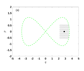
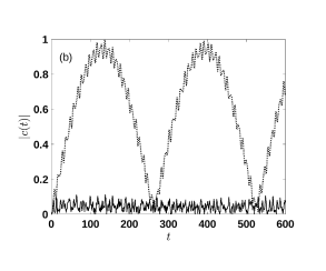
Figure 2: (a) Separatrix of $H_{\rm ord}$ in the phase space of the quartic double well with $D=1$ with unoccupied initial conditions indicated by small open circles; the initially occupied Gaussian is displayed by a filled circle. (b) Comparison of numerical results for the absolute value of the autocorrelation function, using a grid of $M=49$ initial conditions shown in panel (a) in the CCS case (solid line) and converged split operator FFT calculations (dotted line).

Secondly, to see if CCS can do better, we now launch a copy of the grid on the right side also on the left side, as displayed in panel (a) of Fig. 3. Both sets of trajectories are uncoupled, as classical mechanics is a local theory, but the coefficients corresponding to the trajectories are coupled. Thus, although all $a$-coefficients on the left are initially zero, they turn non-zero in the course of time and probability density is transferred to the other side, thus describing tunneling almost perfectly as can be seen in panel (b) of Fig. 3, where we have extended the time interval, such that two complete periods of tunneling can be observed.

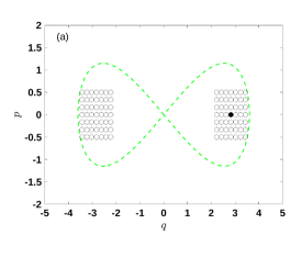
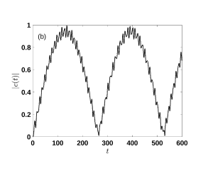
Figure 3: (a) Separatrix of $H_{\rm ord}$ in the phase space of the quartic double well with $D=1$. Dense initial conditions displayed in Fig. 2 and a symmetric copy of those, shifted to the other well; unoccupied initial conditions indicated by small open circles; the initially occupied Gaussian is displayed by a filled circle. (b) Comparison of numerical results for the absolute value of the cross-correlation function, using a grid of $M=98$ initial conditions shown in panel (a) in the CCS case (solid line) and converged split operator FFT calculations (dotted line). Both lines are almost indistinguishable.

As a third try, let us increase the extension of the grid, initially on the right side of the barrier, see panel (a) of Fig. 4. This grid has now 81 points and an extension which is four times as large as the one in panel (a) of Fig. 2, leading to a density still far larger than the von Neumann limit [25], but also leading to a substantial part of initial conditions with energy above the barrier, i.e., outside of the “eight”. The comparison of the autocorrelations in panel (b) of Fig. 4, at least for short times, is now almost as favorable as in Fig. 3. We have not tried to fully converge the results, to still see a little difference between the results plotted in the graph. By retaining the extension of the grid but allowing for 121 instead of 81 trajectories, the quality of agreement with the split operator FFT results is almost as good as in Fig. 3 (not shown). Thus also high energy trajectories “mimic” the tunneling, which happens at low energies quantum mechanically, where there are no classical trajectories (on the left side) by our construction.

This fact is demonstrated in Fig. 5, where the phase space eight, together with the trajectories at time $t=131$, close to half the tunneling period is shown. The trajectories outside of the eight are capable of creating a localized wavepacket at the bottom of the left well (because the overlap with the state $|\beta\rangle$ at the considered time is almost unity. We do not display the relative weight of the trajectories by the size of the dots because, due to the non-orthogonality of the coherent states, the $a$-coefficients are not “normalized” in the same way as the ones in an orthogonal basis expansion and some of them can become exceedingly large. The norm of the wavefunction is conserved to within around one percent for the times displayed in panel (b) of Fig. 4, however.

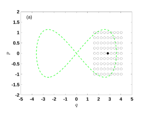
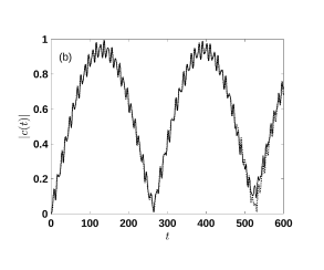
Figure 4: (a) Separatrix of $H_{\rm ord}$ in the phase space of the quartic double well with $D=1$. Less dense initial conditions as compared to Fig. 2, unoccupied initial conditions indicated by small open circles; the initially occupied Gaussian is displayed by a filled circle. (b) Comparison of numerical results for the absolute value of the cross-correlation function, using a grid of $M=81$ initial conditions shown in panel (a) in the CCS case (solid line) and converged split operator FFT calculations (dotted line).

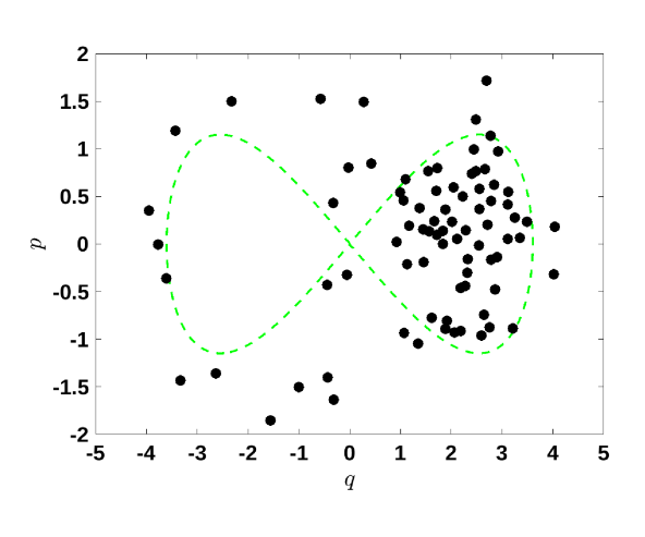
Figure 5: Separatrix of $H_{\rm ord}$ in the phase space of the quartic double well with $D=1$. Snapshot of the time-evolved less dense initial conditions panel (a) of Fig. 4 at time $t=131$ (corresponding to half the tunneling period).

5 Summary and Outlook

We have shown that there are two ways to accurately describe tunneling in a double well by the use of coupled Gaussian basis functions, moving along classical trajectories: (i) either low energy initial conditions for classical trajectories are also launched in the initially unpopulated well, or (ii) one allows for trajectories with enough energy to overcome the barrier. A combination of the two cases has already been studied long ago in [14]. Here we have disentangled the two cases. Due to the fact that the equations of motion for the coefficients are coupled, in the course of time, the $a$-coefficients of all trajectories will start to deviate from zero. Probability density can thus build up in the other well by two scenarios. Either the trajectories have been seeded in the initially unpopulated well from the very start, or they move there by having enough energy. The use of rectangular grids is not mandatory. We believe that also circular grids will do the job [26].

Furthermore, also the investigation of incoherent barrier tunneling is a worthwhile topic. In [27], it has, e.g., been shown that employing classical trajectories in a purely semiclassical (van Vleck-type) study does not lead to converged results for the barrier transmission as a function of the initial wavepacket center, while in [28], the use of multiple spawning of new classical trajectories after time-slicing was shown to lead to converged results. In future work, the use of trajectories that start on one side of the barrier with enough energy to overcome it classically in a CCS study shall be contrasted with the use of trajectories starting on both sides of the barrier. In addition, the investigation of dynamical tunneling [29] in the light of our present findings is left for future research.

Finally, a lot of work on higher-dimensional tunneling applications using Gaussian wavepackets has been performed [30, 31, 32, 33], trying to reduce the number of basis functions as well as to overcome potential problems like zero-point energy leakage of the underlying classical trajectories. Although even in a HK approach it has been shown that the final result is not plagued by zero-point energy leakage [34], for the numerics this might be an issue. The results presented here may give further guidance in the search for efficient numerical algorithms also for more than a single degree of freedom.

References

References

- [1] Beck M, Jaeckle A, Worth G and Meyer H D 2000 Phys. Rep. 324 1 – 105
- [2] Lubich C 2008 From Quantum to Classical Molecular Dynamics: Reduced Models and Numerical Analysis Zurich Lectures in Advanced Mathematics (Zürich: European Mathematical Society)
- [3] Richings G W, Polyak I, Spinlove K E, Worth G A, Burghardt I and Lasorne B 2015 Int. Rev. in Phys. Chem. 34 269–308
- [4] Werther M, Loho Choudhury S and Grossmann F 2021 Int. Rev. in Phys. Chem. 40 81
- [5] Kramer P and Saraceno M 1981 Geometry of the time-dependent variational principle in quantum mechanics (Berlin: Springer Verlag)
- [6] Haegeman J, Cirac J I, Osborne T J, Pizorn I, Verschelde H and Verstraete F 2011 Phys. Rev. Lett. 107(7) 070601
- [7] Schollwöck U 2011 Annals of Physics 326 96 – 192
- [8] Glauber R J 1963 Phys. Rev. 131(6) 2766–2788
- [9] Herman M F and Kluk E 1984 Chem. Phys. 91 27
- [10] Wang Z X and Heller E J 2009 J. Phys. A 42 285304
- [11] Ray S, Ostmann P, Simon L, Grossmann F and Strunz W T 2016 J. Phys. A 49 165303
- [12] Simon L and Strunz W T 2014 Phys. Rev. A 89(5) 052112
- [13] Lando G M, Vallejos R O, Ingold G L and de Almeida A M O 2019 Phys. Rev. A 99(4) 042125
- [14] Shalashilin D V and Child M S 2001 J. Chem. Phys. 114 9296
- [15] Shalashilin D V and Child M S 2000 J. Chem. Phys. 113 10028
- [16] Hund F 1927 Z. Phys. 43 805–826
- [17] Kurkijärvi J 1972 Phys. Rev. B 6 832
- [18] Kierig E, Schnorrberger U, Schietinger A, Tomkovic J and Oberthaler M K 2008 Phys. Rev. Lett. 100 190405
- [19] Grossmann F, Jung P, Dittrich T and Hänggi P 1991 Zeitschrift für Physik B 84 315
- [20] Reichl L E 2004 The Transition to Chaos: Conservative Classical Systems and Quantum Manifestations 2nd ed (New York: Springer)
- [21] Dittrich T and Pena Martínez S 2020 Entropy 22 1046
- [22] Loho Choudhury S and Grossmann F 2022 Phys. Rev. A 105 022201
- [23] Shalashilin D V and Burghardt I 2008 J. Chem. Phys. 129 084104
- [24] Grossmann F 2018 Theoretical Femtosecond Physics: Atoms and Molecules in Strong Laser Fields 3rd ed (Springer International Publishing AG)
- [25] von Neumann J 1955 Mathematical Foundations of Quantum Mechanics (Princeton: Princeton University Press)
- [26] Schleich W P 2001 Quantum Optics in Phase Space (Berlin: Wiley-VCH)
- [27] Grossmann F and Heller E J 1995 Chem. Phys. Lett. 241 45
- [28] Grossmann F 2000 Phys. Rev. Lett. 85 903
- [29] Davis M J and Heller E J 1981 The Journal of Chemical Physics 75 246–254
- [30] Wu Y and Batista V S 2004 J. Chem. Phys. 121 1676–80
- [31] Sherratt P A, Shalashillin D V and Child M S 2006 Chemical Physics 322 127–134
- [32] Saller M A C and Habershon S 2017 J. Chem. Theory Comput. 13 3085
- [33] Dutra M, Wickramasinghe S and Garashchuk S 2020 J. Phys. Chem. A 124 9314–9325
- [34] Buchholz M, Fallacara E, Gottwald F, Ceotto M, Grossmann F and Ivanov S D 2018 Chem. Phys. 515 231