Quantum Monte Carlo and perturbative study of repulsive two-dimensional Bose-Fermi mixtures
Abstract
We derive analytically the leading beyond-mean field contributions to the zero-temperature equation of state and to the fermionic quasi-particle residue and effective mass of a dilute Bose-Fermi mixture in two dimensions. In the repulsive case, we perform quantum Monte Carlo simulations for two representative bosonic concentrations and equal masses, extending a method for correcting finite-size effects in fermionic gases to Bose-Fermi mixtures. We find good agreement between analytic expressions and numerical results for weak interactions, while significant discrepancies appear in the regime close to mechanical instability, above which we provide evidence of phase separation of the bosonic component.
I Introduction
Quantum mixtures have attracted considerable interest in recent years. Thanks to their versatility and tunability they turned out to be an ideal platform to test and develop new physics [1]. In particular, Bose-Bose (BB) mixtures and Fermi-Fermi (FF) mixtures have been studied in depth both from a theoretical and experimental point of view, resulting in a better understanding of important quantum phenomena such as fermionic superfluidity and the BCS-BEC crossover in FF mixtures [2, 3] or self-bound quantum droplets in BB mixtures [4, 5].
Bose-Fermi (BF) mixtures have also been investigated, although somewhat less extensively in the literature. Initial theoretical studies of BF mixtures considered the problem of instability (by collapse or phase separation) using mean-field and perturbative approaches, emphasizing the need for a sufficiently high repulsive interaction between bosons [6, 7, 8]. The occurrence of instabilities was also confirmed experimentally by the first realization of a non-resonant BF mixture [9]. Later, with the development and refinement of more sophisticated techniques such as optical lattices and Feshbach resonances [10, 11], the focus shifted to strongly interacting Bose-Fermi systems. Indeed, the possibility to tune the interaction between bosons and fermions by varying an external magnetic field has ensured different possible implementation scenarios.
The case of a Bose-Fermi mixture with a BF interaction modulated by a Feshbach resonance has attracted particular interest in the literature. Initial works studying this system in the presence of a resonance focused on lattice models [12, 13, 14]. Subsequent works moved instead to the continuous case [15]. In addition to the instability problem [16, 17], the competition between BF pairing and boson condensation in a Bose-Fermi mixture across a broad Feshbach resonance was studied in [18, 19, 20]. In particular, it was found that for weak attraction, at sufficiently low temperature, the bosons condense while the fermions behave like a Fermi liquid. Instead, for sufficiently strong attractions, bosons and fermions pair into molecules. Parallel to theoretical studies, boson-fermion Feshbach molecules were achieved also experimentally. The first realizations were obtained in Hamburg [21] and in Boulder [22] with mixtures. Later, the creation of Feshbach molecules was achieved also with an isotopic mixture [23], as well as with [24], [25], [26], , and [27] heteronuclear BF mixtures. Recently, Feshbach molecules have been successfully transferred to the absolute molecular ground state and cooled down to quantum degeneracy [28], while Ref. [29] has investigated the same mixture across the whole broad Feshbach resonance between bosons and fermions, confirming theoretical predictions [20] about a universal behavior of the condensate fraction and the occurrence of a quantum phase transition.
Equally interesting is the case of repulsive Bose-Fermi mixtures, which are characterized by both intra- and inter-species repulsive interactions. The formation of Feshbach molecules is here prohibited by the repulsive nature of the interactions. However, the problem of instability persists: sufficiently large repulsive boson-fermion interactions lead the system towards phase separation [8, 30, 31, 32].
The possibility of confining mixtures in lower dimensions using optical potentials elicited interest in two-dimensional (2D) mixtures. Besides the intrinsic interest of many-body systems in reduced dimensionality, the presence of a confining potential offers a further knob to tune the effective 2D interactions between the components of the mixture through a confinement-induced resonance [33, 34, 35, 36]. Interestingly, it has been shown in Ref. [37] that such a mechanism in 2D could lead to the creation of collisionally stable fermionic dimers made by one boson and one fermion, with a strong p-wave mutual attraction that could support a p-wave superfluid of dimers. Besides this recent important result, relatively few theoretical studies have been conducted on 2D BF mixtures [38, 39, 40, 41, 42, 43].
This motivates the present paper, in which we present a combined effort of a (second-order) perturbative study and numerical non-perturbative quantum Monte Carlo (QMC) simulations of repulsive 2D Bose-Fermi mixtures, investigating the regime of validity of perturbation theory and the onset of phase separation.
Our main results are: i) The derivation of the fermionic effective mass at the perturbative level and with a QMC estimation employing a novel finite-size extrapolation method; ii) The detailed analysis of the equation of state, with varying BF repulsion and bosonic concentration, for which we observe good agreement between perturbative and QMC results up to the predicted onset of phase separation; iii) The study of this onset from a stability condition viewpoint, and by inspection of QMC pair correlation functions.
The article is organized as follows. In Sec. II we develop the perturbative theory up to second order, deriving an expansion for the chemical potentials and equation of state, the effective mass, and the stability condition. In Sec. III we describe the Monte Carlo methods that we used, including a new finite-size correction scheme for BF mixtures, and report our results for the effective mass, the equation of state, and the bosonic pair distribution function for different bosonic concentrations. Finally, Sec. IV reports our conclusions.
II Perturbative expansion
We consider a 2D BF mixture with fermionic particle density and bosonic particle density , where is the bosonic concentration. The atomic masses are and , respectively, where we introduced the mass ratio . We are interested in developing a perturbative treatment for Bose-Fermi mixtures. Previous perturbative works have indeed studied Bose-Fermi mixtures only in three dimensions [44, 45] while only Fermi-Fermi [46, 47, 48, 49, 50, 51] or Bose-Bose systems [52, 53, 54, 55, 56, 57] have been considered in two dimensions. Our perturbative treatment will be valid for generic mass-imbalanced mixtures, for both attractive and repulsive BF interactions, while we will focus on the repulsive case with equal masses () in the QMC simulations.
II.1 Diluteness condition and expansion parameters
We assume the system to be dilute, such that the average distance between any pair of particles of the mixture is much larger than the range of their interaction. Under this condition, the boson-fermion and boson-boson interactions can be parametrized in terms of the corresponding (2D) -wave scattering lengths and , while fermion-fermion interactions can be altogether neglected since -wave interactions between identical fermions are forbidden by Fermi statistics and direct -wave (or higher angular momenta) interactions are strongly suppressed.
Specifically, for a generic finite-range two-body interaction, the -wave phase shift, which yields the dominant contribution to the scattering amplitude at low relative momenta , has the following effective-range expansion in 2D for approaching zero (see, e.g., [58, 59]):
| (1) |
where the length appearing within the logarithm defines the -wave scattering length, and the constant finite terms in the limit have been included in its definition. With this convention, the 2D scattering length of a hard-disk potential of radius is , where is Euler-Mascheroni constant, while, in the attractive case, the dimer binding energy is , where is the reduced mass. An alternative convention (used for example in Refs. [60, 61, 62, 63]) would correspond to for a hard-disk potential.
In the repulsive case, the scattering length is of the same order of the range of interaction (for a strong barrier) or even much smaller than (for a weak barrier). The diluteness condition then automatically implies that the gas parameters and are much smaller than 1. Actually, in two dimensions, due to the logarithmic dependence of the scattering amplitude on the relative momentum and energy, it is convenient to describe boson-boson and boson-fermion interactions in terms of the dimensionless coupling parameters and , where the Fermi momentum is related to the fermion density by the equation .
For attractive BF interaction, the scattering length coincides with the bound-state radius, and is not necessarily related to the range of the interaction (the range can even be vanishing in this case). Perturbation theory requires in this case , corresponding to a weakly-bound two-body bound state with a large radius compared with the average interparticle distance and implying that is small and negative. The BF system is thus dilute with respect to the range () but dense with respect to the bound state radius (). These differences notwithstanding, perturbation theory is formally identical in the two cases.
In both cases, our perturbative expansion is constructed by considering and of the same order, say and , where and are some numerical constant, and taking the limit . We will be interested in particular in deriving a perturbative expansion to second order in the small parameter .
For brevity, in the rest of this section we set .
II.2 Many-body T-matrix
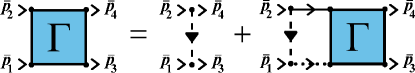
The basic building block of perturbation theory for a dilute Bose-Fermi mixture is the generalization to the many-body system of the two-body T-matrix. The many-body T-matrix can be interpreted as a generalized scattering amplitude in the medium, accounting for the influence of the other particles in the scattering processes. In terms of Feynman’s diagrams, it is the sum of ladder diagrams (see Fig.1) and, in 2D, it corresponds to the following integral equation:
| (2) |
Here, overbarred quantities indicate -vectors: , where is a momentum variable and is a frequency; is the Fourier transform of the interaction potential between bosons and fermions at distance , while the bare boson and fermion Green’s functions at zero temperature are given by
| (3) | |||||
| (4) |
where is an infinitesimal positive quantity and is the boson chemical potential. Translational invariance and the instantaneous nature of the interaction potential imply that the many-body T-matrix depends on three momenta and one frequency. In particular, by defining , and integrating over the frequency in Eq. (II.2), one obtains
| (5) |
For vanishing densities, such that , the above equation reduces to the integral equation for the two-body T-matrix of the quantum theory of scattering [cf. Eq.61 of appendix A] calculated at , where , and the reduced mass .
The on-shell two-body -matrix, , is instead obtained by calculating for , such that
| (6) |
In analogy with the 3D case, the similarity in the structure of Eqs. (5) and (6) allows one to replace with in the integral equation (5) (see, e.g. [64, 44]), yielding:
| (7) |
which is the starting point for our perturbative calculations. In particular, a perturbative expansion in the small parameter (see appendix B for details) shows that to second order in the many-body T-matrix depends only on the total 3-momentum , then yielding with
| (8) |
where the dimensionless function is defined by Eqs. (75) and (76) of appendix B. Note that the expansion (8) is valid both in the repulsive () and attractive () cases.
Equation (8) clearly shows that is the basic building block of the perturbative expansion with respect to the boson-fermion coupling parameter .
II.3 Fermionic self-energy and chemical potential
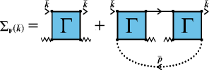
To second order in the small parameter , only the two diagrams shown in Fig. 2 contribute to the irreducible fermionic self-energy . It is indeed clear from Eq. (8) that diagrams containing three or more would contribute only to order or higher. In the same way, diagrams obtained by replacing in the first diagram of Fig. 2 the two condensate factors with a bosonic line dressed by self-energy insertions (including anomalous terms) contribute only higher order terms in the small parameter , apart for a term of order originating from the condensate depletion induced by the boson-boson interaction. This term is automatically taken into account by replacing with in the diagrams of Fig. 2. Note further that the diagram obtained by the second diagram of Fig. 2 by replacing the dotted line with two condensate insertions is reducible and thus does not contribute to the irreducible self-energy.
In order to calculate perturbatively the fermionic chemical potential , as well as the quasi-particle residue and fermionic effective mass , we need in a neighborhood of , where is the Fermi energy in the absence of interactions. In this region, the self-energy is given by (see appendix C for details):
| (9) |
where , , , and .
The chemical potential is most easily obtained from the self-energy by using Luttinger’s theorem [65], which connects the fermionic chemical potential to the real part of the self-energy calculated at the Fermi momentum and frequency :
| (10) |
By noticing that the self-energy (9) depends on the frequency only through the term proportional to and that , one sees that, neglecting terms of order higher than , Eq. (10) can be replaced with
| (11) |
By setting in (9) and (such that and ), one obtains
| (12) |
yielding
| (13) |
where and we used . For equal masses, by taking the limit , Eq. (13) reduces to
| (14) |
II.4 Ground-state energy and bosonic chemical potential
The ground-state energy per unit volume can be obtained by integrating the chemical potential over the fermion density from 0 to :
| (15) |
where is the ground-state energy per unit volume of the boson component in the absence of fermions. We make the dependence of on in Eq. (13) more explicit
| (16) |
where depends on via and
Integration by parts of the terms depending on in Eq. (16) yields
| (17) | |||||
| (18) |
Neglecting terms of order higher than , we thus obtain
| (19) |
We emphasize that, according to our expansion, Eq. (19) is valid to order , that is, neglecting terms of order higher than two in , , or their combinations. Under this assumption, terms involving simultaneously and do not contribute to .
In the mass-balanced case on which we will focus in our QMC simulations, Eq. (19) reduces to
| (20) |
We will verify, in particular, the validity of the term proportional to in Eq. (20), which is the novel contribution to the equation of state derived by our perturbative calculation.
Concerning instead the bosonic term , an accurate perturbative expansion has been obtained in [57], and verified with QMC calculations shortly after [60]. Its expression is
| (21) |
where , and with our convention for the scattering length. Neglecting terms of order higher than , consistently with the order of our perturbative calculation, the above equation reads
| (22) |
Coming back to expression (19) for the ground-state energy of the Bose-Fermi mixture, differentiation with respect to yields immediately the bosonic chemical potential
| (23) |
where is the boson chemical potential in the absence of fermions. Neglecting terms of order higher than , it is given by
| (24) |
For equal masses, Eq. (23) reduces to
| (25) |
II.5 Quasi-particle residue
The quasi-particle residue is obtained by the relation:
| (26) |
Since and the self-energy (9) depends on the frequency only through the term proportional to , one would be tempted to evaluate the derivative with respect to in the above equation for . Such a derivative is however divergent as , and so it is important to evaluate it at rather than .
Indeed, by setting (corresponding to ) in Eq. (9), and analyzing separately the behavior of for and one obtains the following asymptotic behavior for when (corresponding to ):
| (27) |
which clearly shows that diverges as for .
By inserting expression (13) for in Eq. (27) and neglecting terms , we obtain
| (28) |
where in the last line we have used and . Note that due to the divergence of for , the leading term in the expansion for is proportional to rather than , as one would get in the absence of such a divergence (and as it occurs e.g. in a Fermi-Fermi system [46, 48]).
Mathematically, this diverging derivative originates from the presence of a Fermi step function in the integral over momentum yielding the second-order term for . In a Fermi-Fermi system this divergence is smeared by a further integral over momentum and frequency, which is absent in the BF mixture because a fermionic line with arbitrary momentum and frequency is replaced with a condensate line with vanishing momentum and frequency.
II.6 Effective mass
The effective mass is obtained by the relation:
| (29) |
By setting in Eq. (9) and taking the derivative with respect of , one obtains
| (30) |
such that, by inserting Eqs. (30) and (28) in Eq. (29):
| (31) |
which, for equal masses (), reads:
| (32) |
Note again that the leading term in the expansion for is proportional to rather than , a behavior which is directly inherited from the quasi-particle residue .
II.7 Mechanical stability
Mechanical stability requires the compressibility matrix (with ) or, equivalently, its inverse , to be positive definite [6]. It corresponds to
| (33) |
and
| (34) |
The second inequality, using the symmetry of the compressibility matrix, reads
| (35) |
which, when satisfied, makes the inequality (33) to be respected automatically in both cases () when it is verified for just one of them. One has (always neglecting higher order terms)
| (36) | ||||
| (37) | ||||
| (38) |
One sees that always. We thus need to satisfy only (35) for the stability of the Bose-Fermi mixture. When using Eqs. (36)(38), it reads
| (39) |
which, for equal masses, reduces to
| (40) |
The condition (39) can be simplified if one keeps only the leading order terms, corresponding to a “mean-field" treatment of the BB and BF interaction. At this level of approximation one obtains
| (41) |
which, for equal masses, reduces to
| (42) |
The condition for stability (41) is the counterpart for a 2D Bose-Fermi mixture of the analogous condition for stability in 3D obtained in [6], which can be written as
| (43) |
Both condition (41) in 2D and condition (43) in 3D can be interpreted as the requirement that the direct BB repulsion overcomes the effective attraction between bosons induced by interactions with fermions, in such a way that the overall effective interaction between bosons remains repulsive [66]:
| (44) |
Here and are the leading order expression in the weak-coupling limit of the T-matrices for BB and BF interactions, and are given by
| (45) |
in 2D and by
| (46) |
in 3D, while is the compressibility of the ideal Fermi gas, which is given by
| (47) |
in 2D and by
| (48) |
in 3D. It is straightforward to verify that conditions (41) and (43) are obtained from condition (44) when Eqs. (45), (47) or (46), (48) are used, respectively.
III Quantum Monte Carlo
III.1 Method
To determine the ground state properties of a repulsive 2D Bose-Fermi mixture, we employ two different QMC techniques: variational Monte Carlo (VMC) and diffusion Monte Carlo (DMC). The VMC method stems from the application of Monte Carlo integration to the evaluation of quantum expectation values in chosen and suitably optimized variational trial wavefunctions , and it is designed to be directly applied to both bosonic and fermionic systems [67, 68]. Diffusion Monte Carlo is instead a more sophisticated technique that allows for a stochastic solution of the many-body Schrödinger equation in imaginary time. It is in principle an exact method for bosonic systems, but in the presence of fermions the sign problem arises. We use the standard fixed-node approximation, which consists in imposing that the nodal surface of the true many-body wave function is the same as the one of the trial wave function employed in our VMC simulations [69]. Thus, both techniques provide an upper bound to the true ground state energy [70], which can be lowered by variationally optimizing .
The considered system is described by an effective low-energy Hamiltonian, which is set to reproduce the scattering lengths of the full atomic problem. Its expression is the following:
| (49) |
where and label, respectively, fermions and bosons, and are their numbers, and is the distance between particles and . The short-range fermion-fermion interaction can be neglected at low energies due to the Pauli exclusion principle, while the specific form of the interaction potentials, and , is irrelevant in the dilute regime of interest for ultracold gases. In particular, we assume a soft-disk potential for both interactions: for and zero elsewhere, and similarly for , and parametrize the strength of the interactions and in terms of their respective scattering lengths, according to the relation [71] where the subscript indicates the or pair, , is the reduced mass of the pair and is the modified Bessel function of order . In this work, we tune both and so that the right-hand side of the former relation is equal to . The results for the observables depend only on the scattering lengths, provided that the bare radii of the model potentials, and , are negligible when compared to the densities of the two components: and . For the BB radius, we have set . The value of changes according to and is smaller than in the homogeneous phase.
Simulations are carried out in a square box of area with periodic boundary conditions (PBC), with a number of fermions up to and a number of bosons depending on the targeted bosonic concentration . We focus on the case of equal masses, thus . We use a Jastrow-Slater trial wavefunction, which turned out to be a good ansatz in the three-dimensional case [72, 73, 20]. Thus, is given by the product of two terms: and . is a function of the particle coordinates which is symmetric upon exchange of any two fermions or two bosons, and contains information regarding the boson-boson and the boson-fermion correlations. In the Jastrow form, this term reads as , where the functions describe the two-body correlations and are solutions of the two-body problem with suitable boundary conditions. In particular, PBC require null first derivative of at distance . For this reason, we introduce two variational parameters and , to be optimized, that allow one to parametrize the distance at which the two-body Jastrow correlations go to a constant, with null first derivative [71]. The second term, , satisfies the fermionic antisymmetry condition and determines the nodal surface of . In particular, we use a Slater determinant made of single particle orbitals in the form of plane waves, whose wavevectors are , where and are integer numbers. As customary, these wavevectors are chosen so as to fill closed shells, which are closed with respect to mirror and discrete rotational symmetries, in order to reduce finite-size effects. The optimized is then obtained by choosing the pairs of parameters and so as to minimize the VMC ground state energy.
III.2 Finite-size analysis
In order to make simulations computationally affordable, it is necessary to limit the study to systems with a relatively small number of particles. This implies inaccuracies in the QMC results, due to finite-size effects, with respect to the thermodynamic limit. To reduce them, we extend a finite-size correction originally developed in the case of Fermi mixtures [74, 75, 76] to the case of Bose-Fermi mixtures. We assume that the finite-size correction related to the purely bosonic component is negligible, since we focus on relatively small bosonic concentrations, and the fermionic finite-size effects are presumably much more relevant due to shell effects.
We consider that the fermions do indirectly interact via the mediation of bosons. This allows us to use Landau Fermi liquid theory to elaborate an extrapolation scheme to the thermodynamic limit. In this approach, we assume that the main finite-size correction is analogous to the one of a noninteracting Fermi system, which is a purely kinetic energy contribution, introducing the equation:
| (50) |
where and are the energies per fermion of the finite system with PBC and of the infinite system with the same fermion density and boson concentration , respectively, while is the energy difference per fermion between a system of noninteracting fermions in the same square box with PBC and the infinite system with the same fermion density , which is easily tabulated. The parameter can be identified as the inverse of the effective mass and can be determined by fitting the QMC data obtained for different values of , in analogy with the Fermi mixture case [74, 75, 76]. Notice that, since interaction in this Fermi liquid is mediated by bosons, the term depends both on the fermionic density and on the bosonic concentration . Unfortunately, it is not possible to perform simulations with different and , which vary discretely, while keeping constant . Thus, simulations with different also correspond to different , which we are not free to consider as an independent variable. This prompts us to expand around a reference bosonic concentration in terms of the variation . We therefore introduce the following scaling equation:
| (51) |
where the first term is the contribution of a gas of noninteracting fermions in the thermodynamic limit, while is the energy per boson of the corresponding interacting system of bosons in the absence of fermions, for which we can use the accurate equation of state [60] given by expression (21). Since we assume that finite size effects of the purely bosonic contribution are negligible with respect to the fermionic ones, the energy per boson is also taken in the thermodynamic limit. The remaining parameters , and are obtained by fitting QMC results and model the residual correlation energy in the vicinity of . The above functional form is not the only possible choice for correcting for finite-size effects. In fact, we tested alternative expansions, for example by introducing contributions explicitly depending on inverse powers of , and we realized that the parameter is quite stable with respect to the different fitted functional forms, while Eq. (51) allows us to obtain reasonable values for the reduced chi-square.
We fitted the above scaling equation to VMC data, obtaining the effective mass and thus a finite-size correction for each considered BF interaction value, that we later applied to correct DMC results using the expression . For some test case we applied the same fitting technique also to DMC data, and observed that the resulting effective masses were compatible. We attribute this to a prominent role of the nodal surface in determining the effective mass. Previous studies on the electron gas indeed showed an important role of backflow correlations in the Slater determinant [75, 77]. In the context of BF mixtures, this suggests a relevant future research direction, together with the comparison to other effective-mass calculation approaches within QMC methods, such as the evaluation of imaginary-time diffusion of quasiparticles [78], the explicit simulation of finite-momentum wavefunctions [79], or the methodology recently introduced in [80] based on the calculation of the static self-energy.
III.3 Results
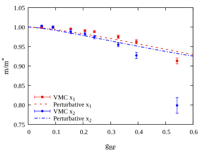
In this work, we focus on two reference bosonic concentrations and , which represent mixtures with small and high bosonic densities, respectively. The results for the effective masses are shown in Fig. 3. They are obtained from the fitting scheme described in Sec. III, using and numbers of bosons chosen so as to get concentrations close to the two reference concentrations and , respectively. In the low interaction regime, the QMC results for both concentrations barely differ from the noninteracting value . For increasing interaction, although the QMC results qualitatively follow Eq. (32), some discrepancy between the perturbative predictions and the QMC points is manifest. This might be due to a not sufficiently accurate nodal surface, which could be improved by introducing backflow correlations. For the disagreement is even more evident. This could be related both to the deficiency of perturbation theory in the strongly interacting regime, and to the limits of our extrapolation scheme for strong BF interactions, where, presumably, fermions can no longer be described with Fermi liquid theory. In fact, in such regime phase separation is expected, and the homogeneous Fermi liquid is at best only a metastable state.
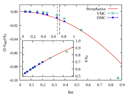
We now discuss the zero-temperature equation of state for the two considered bosonic concentrations. When comparing the perturbative prediction (19) for the ground state energy with our QMC results, we find it convenient to consider the energy per fermion . In addition, to better visualize the contribution of the term proportional to in the perturbative expansion, we write where the “mean-field” term
| (52) |
includes the non-interacting ground-state energy of the Fermi component, its mean-field correction due to interaction with bosons, as well the ground-state energy of the boson component in the absence of interaction with fermions (all divided by ). With this definition, our perturbative expression (20) yields for the term the expression
| (53) |
to order .
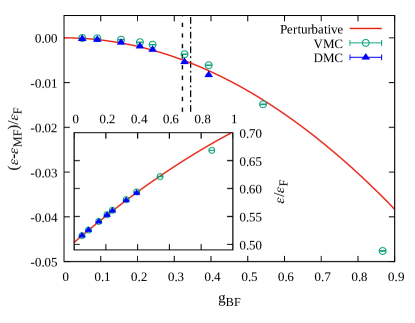
Our QMC results for the beyond mean-field correction , in units of the Fermi energy , are shown in Figs. 4-5, together with the perturbative prediction (53). The shown VMC and DMC results are obtained with a number of fermions and they are corrected from finite-size errors using the procedure described above. Furthermore, the DMC energies are the result of proper time-step and walker population analyses. The QMC results are in agreement with the analytic perturbative predictions for small BF interaction values. In particular, for the smaller bosonic concentration , DMC results agree with the perturbative expansion for while in the case of agreement is found only for . We also indicate the perturbative stability conditions of the mixture (42) with vertical lines: dot-dashed for the mean-field condition of Eq. (42), and dashed for the second-order condition of Eq. (40). For stronger interactions, at the perturbative level the mixtures lose their homogeneity. Consequently, one would expect that this regime can no longer be efficiently simulated with a translationally invariant and isotropic Jastrow-Slater wavefunction, such the one that we employ. This is the reason why we do not perform DMC simulations for .
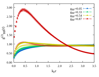
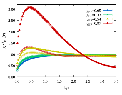
The instability predicted by the perturbative results was indeed experienced during our DMC simulations, as we now describe by performing a qualitative analysis of the BB pair distribution function . The results are shown in Figs. 6-7, for two different bosonic concentrations. VMC and DMC results are compared with each other, for different values of the BF coupling.
Since the DMC estimator for pair distribution functions is not pure but mixed, meaning that it is affected by the used trial wavefunction, usually an extrapolation from the VMC and DMC results is performed, which is valid when their differences are small, or the forward walking technique is used [81]. Here, instead, we use the discrepancies between the DMC and VMC results as an indication of how suited the employed trial wavefunction is to describe the true groundstate. For both concentrations, and small BF interactions, the BB repulsion suppresses the probability of finding two bosons close to each other. By increasing the distance, the probability density increases until it reaches a plateau value, corresponding to a homogeneous system. This behavior is, in fact, observed for . For stronger BF repulsion, the shape of the BB pair distribution function starts to change drastically, presenting a peak for distances less than and a probability density that decreases for larger distances. Indeed, if the BF repulsion is strong enough, the presence of an effective attraction between the bosons is expected, thus leading to the formation of bosonic clusters. This behavior is much more evident in the DMC results, where the system has evolved towards the true ground state containing the bosonic clusters. Here, the very large discrepancy between the VMC and the mixed DMC estimators points to a state that is significantly different from the employed Jastrow wavefunction, which is translationally invariant and isotropic, since it includes only factors that depend on relative distances. In this inhomogeneous regime, one must be aware that finite-size effects might be significant. The main difference between the two considered boson concentrations is in the prominence of the cluster peaks, which highlights that the higher the concentration the stronger the effect.
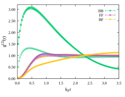
To further analyze the clustering behavior of the system, in Fig. 8 we also report the FF and BF pair distribution functions, respectively and , for the strong BF repulsion , by simulating fermions and bosons, corresponding to concentration . The BB pair distribution function shows typical clustering phenomenology, as discussed above. is instead very similar to the non-interacting case, which is expected, since fermions are the majority species in this mixture and their compressibility is limited by Fermi pressure. Still, the mixed DMC estimator of manifests slightly enhanced oscillations compared with the VMC one. Another convincing hint of clustering comes from the shape of the mixed DMC estimator of . A shift in probability towards greater distances between bosons and fermions can be observed, which is further evidence of a reduced uniformity of these two components. All these considerations qualitatively confirm the presence of phase separation for strong BF repulsion.
IV Conclusions
In this work we filled a gap in the theory of 2D dilute BF mixtures by deriving the leading beyond-mean-field contributions to the equation of state, as well as to the fermionic quasi-particle residue and effective mass. For equal masses, and in the repulsive case we have performed QMC simulations, extending to BF mixtures a procedure to correct finite-size effects which was previously used for Fermi-Fermi systems. Our QMC results validate the beyond-mean-field perturbative expansion for the equation of state up to moderate BF repulsion, depending on the bosonic concentration.
The perturbative expansion for the quasi-particle residue and effective mass contains a non-analytic term in the BF coupling (proportional to ) that is absent in the corresponding expansion for a two-component Fermi system [46, 48] and which originates from the presence of a condensate in the BF mixture. For the effective mass, we have attempted comparison with the effective mass extracted from our procedure to correct finite-size effects of QMC simulations, finding in this case only qualitative agreement. Future work will be devoted to increasing the accuracy of the effective mass from QMC simulations of Bose-Fermi mixtures.
We also investigated the onset of phase separation in repulsive BF mixtures, as predicted by perturbative theory and demonstrated by clustering in the nonperturbative bosonic pair distribution function. While the two results are in qualitative agreement, further work is needed, aiming at quantitatively characterizing the transition from the nonperturbative energetic point of view. This will require a systematic evaluation of the QMC equation of state for different bosonic concentrations in the uniform phase, in order to evaluate a fully nonperturbative stability condition.
Another important research direction will be the verification of the universality of the QMC results, which are here based on a single soft-disk potential, whose effective range could become relevant in the strongly repulsive regime. In particular, while with our model potential we have before the onset of phase separation, deep in the phase-separated state results can depend on the chosen repulsive model. This is also a regime where in a real atomic system effective repulsion is accompanied by the possible presence of bound states of the full interatomic potential, so that the competition between the phase-separated state and the molecular instability has to be investigated (a problem analogous to the stability of itinerant ferromagnetism in Fermi mixtures [82]). Nevertheless, the good agreement between the perturbative and DMC results for the equation of state up to the predicted perturbative phase-separation coupling hints at a negligible role of nonuniversal effects in the uniform phase.
Data for reproducing the figures are available online [83].
Acknowledgements.
We acknowledge the use of computational resources from the parallel computing cluster of the Open Physics Hub at the Physics and Astronomy Department in Bologna. We acknowledge the CINECA award IscrC-BF2D (2021), for the availability of high performance computing resources and support. P.P. acknowledges financial support from the Italian Ministry of University and Research under project PRIN2022 No. 2022523NA7 and from the European Union - NextGenerationEU through the Italian Ministry of University and Research under PNRR - M4C2 - I1.4 Project CN00000013.Appendix A Quantum scattering theory in two dimensions: main equations
We report here the main equations from quantum scattering theory in two dimensions since the 2D case is less standard than the 3D one and notations and definitions are scattered in the literature (and sometimes differ from author to author).
The scattering amplitude from the incoming wavevector to the outgoing wavevector is defined from the asymptotic behavior of the stationary scattering wave function at large distance from the potential center:
| (54) |
where for elastic scattering (see e.g. [58]). With this definition, the differential cross section, like in 3D, is given by
| (55) |
where is the angle between and The 2D partial-wave expansion reads
| (56) | |||||
| (57) |
At low energies for , while (see, e.g., [59, 58])
| (58) |
We then see that, like in 3D, the s-wave scattering dominates at low energies, so that
| (59) |
The scattering amplitude can be connected to the on-shell two-body -matrix , defined by the equation
| (60) |
Here, the (off-shell) two-body -matrix is defined as the solution of the Lippmann-Schwinger equation
| (61) |
where , is the reduced mass, is in general a complex energy, and is the Fourier transform of the scattering potential . In two dimensions, the connection between and is given by the relation [58]
| (62) |
Note that, while for the scattering amplitude as defined by Eq. (54) one has , for the -matrix one has in general .
Appendix B Perturbative expansion of the many-body T-matrix
In this appendix we derive an expansion for the many-body -matrix describing the interaction between bosons and fermions to second order in the 2D gas parameter . For convenience, we set .
The relevant momenta in our dilute system are of the order of the Fermi momentum , which is small in comparison with the momentum scale set by the range of the BF interaction. We can thus use the low-momenta expression (63) for the on-shell two-body -matrix. Moreover, by introducing the dimensionless momentum variable and using the perturbative assumption , one has
| (64) | |||||
| (65) |
where we have used that is the dominant term in the denominator (for both attractive and repulsive cases).
Recalling Eq. (II.2) for the many-body -matrix , and expanding it to second order in , one obtains
| (66) |
where has been set to zero within the integral on the left-hand side of Eq. (66), consistently with the order of our calculations. We observe that, since the two-body -matrix at low energy depends only on the (magnitude) of the incoming momentum , the many-body -matrix does not depend on the outgoing relative momentum . A change of variable followed by a transformation to polar coordinates yields
| (67) |
where we have introduced the dimensionless variables , , and .
Integration over the angle yields
| (68) |
with and real. In the present case
| (69) |
One thus gets
| (70) |
where
| (71) |
Using
| (72) | |||||
| (73) | |||||
one notices that the dependence of on the relative momentum disappears, then yielding with
| (74) |
where
| (75) |
while
| (76) |
and we have defined .
Appendix C Perturbative expansion of the fermionic self-energy
The two Feynman diagrams of Fig. 2 yield two different contributions to the self-energy:
| (77) |
with
| (78) | |||
| (79) |
where we have defined . Let us consider the two terms separately. For the first term, Eq. (74) for yields
| (80) |
where, consistently with the order of the expansion, we have replaced with .
The function is determined by the expressions (75) or (76) (with replaced by ) depending whether the condition
| (81) |
is verified or not (where for convenience we have introduced the dimensionless variables and ).
In order to obtain the chemical potential , the fermion effective mass at , and the quasi-particle weight , it is sufficient to know the self-energy close to and for frequencies in a neighborhood of the energy shell . In this case, is always determined by expression (75). Indeed, exactly on shell ( ) the condition (81) reads
| (82) |
which, for is always verified, while for it is verified for
| (83) |
thus always including a neighborhood of . More generally, even off the energy shell, setting , the condition (81) reads
| (84) |
For , the condition (84) is verified for all if , so it is valid in an extended neighborhood of the energy shell . For , it can be proven that the condition (84) is certainly verified for and , implying that there is always a finite neighborhood of where the condition (84) is verified.
For the term as given by Eq. (79), after integrating over the frequency , replacing with , and with one gets
| (86) |
After the shift , and introducing dimensionless variables:
| (87) |
The integral over is solved by using Eq. (68), yielding:
| (88) |
with
| (89) |
For , is always positive in the range of integration for , a condition that is certainly verified in an extended neighborhood of . For , on the energy shell , is always positive if , which is always verified in a neighborhood of . More generally, even off the energy shell, one can verify that there is a neighborhood of and where is always positive within the range of integration. For the calculation of the physical quantities of interest in this work, we can then replace with in Eq. (88) for all values of and proceed with the calculation of the integral over . By defining , one has
| (90) |
where , , . The integral over is solved by using Eq. (73), yielding
| (91) |
By summing (88) and (C) one finally obtains Eq. (9) of the main text for .
Finally, we report the expression of the self-energy for the specific case of equal masses , which is obtained by taking the limit from the general expression (9)
| (92) |
References
- Bloch et al. [2008] I. Bloch, J. Dalibard, and W. Zwerger, Many-body physics with ultracold gases, Rev. Mod. Phys. 80, 885 (2008).
- Giorgini et al. [2008] S. Giorgini, L. P. Pitaevskii, and S. Stringari, Theory of ultracold atomic Fermi gases, Rev. Mod. Phys. 80, 1215 (2008).
- Strinati et al. [2018] G. C. Strinati, P. Pieri, G. Röpke, P. Schuck, and M. Urban, The BCS–BEC crossover: From ultra-cold Fermi gases to nuclear systems, Phys. Rep. 738, 1 (2018).
- Semeghini et al. [2018] G. Semeghini, G. Ferioli, L. Masi, C. Mazzinghi, L. Wolswijk, F. Minardi, M. Modugno, G. Modugno, M. Inguscio, and M. Fattori, Self-bound quantum droplets of atomic mixtures in free space, Phys. Rev. Lett. 120, 235301 (2018).
- Cabrera et al. [2018] C. R. Cabrera, L. Tanzi, J. Sanz, B. Naylor, P. Thomas, P. Cheiney, and L. Tarruell, Quantum liquid droplets in a mixture of Bose-Einstein condensates, Science 359, 301 (2018).
- Viverit et al. [2000] L. Viverit, C. J. Pethick, and H. Smith, Zero-temperature phase diagram of binary boson-fermion mixtures, Phys. Rev. A 61, 053605 (2000).
- Roth and Feldmeier [2002] R. Roth and H. Feldmeier, Mean-field instability of trapped dilute boson-fermion mixtures, Phys. Rev. A 65, 021603 (2002).
- Roth [2002] R. Roth, Structure and stability of trapped atomic boson-fermion mixtures, Phys. Rev. A 66, 013614 (2002).
- Modugno et al. [2002] G. Modugno, G. Roati, F. Riboli, F. Ferlaino, R. J. Brecha, and M. Inguscio, Collapse of a Degenerate Fermi Gas, Science 297, 2240 (2002).
- Lewenstein et al. [2007] M. Lewenstein, A. Sanpera, V. Ahufinger, B. D. A. Sen(De), and U. Sen, Ultracold atomic gases in optical lattices: Mimicking condensed matter physics and beyond, Adv. Phys. 56, 243 (2007).
- Chin et al. [2010] C. Chin, R. Grimm, P. Julienne, and E. Tiesinga, Feshbach resonances in ultracold gases, Rev. Mod. Phys. 82, 1225 (2010).
- Kagan et al. [2004] M. Y. Kagan, I. V. Brodsky, D. V. Efremov, and A. V. Klaptsov, Composite fermions, trios, and quartets in a Fermi-Bose mixture, Phys. Rev. A 70, 023607 (2004).
- Günter et al. [2006] K. Günter, T. Stöferle, H. Moritz, M. Köhl, and T. Esslinger, Bose-Fermi Mixtures in a Three-Dimensional Optical Lattice, Phys. Rev. Lett. 96, 180402 (2006).
- Barillier-Pertuisel et al. [2008] X. Barillier-Pertuisel, S. Pittel, L. Pollet, and P. Schuck, Boson-fermion pairing in Bose-Fermi mixtures on one-dimensional optical lattices, Phys. Rev. A 77, 012115 (2008).
- Watanabe et al. [2008] T. Watanabe, T. Suzuki, and P. Schuck, Bose-Fermi pair correlations in attractively interacting Bose-Fermi atomic mixtures, Phys. Rev. A 78, 033601 (2008).
- Yu et al. [2011] Z.-Q. Yu, S. Zhang, and H. Zhai, Stability condition of a strongly interacting boson-fermion mixture across an interspecies Feshbach resonance, Phys. Rev. A 83, 041603 (2011).
- Ludwig et al. [2011] D. Ludwig, S. Floerchinger, S. Moroz, and C. Wetterich, Quantum phase transition in Bose-Fermi mixtures, Phys. Rev. A 84, 033629 (2011).
- Fratini and Pieri [2010] E. Fratini and P. Pieri, Pairing and condensation in a resonant Bose-Fermi mixture, Phys. Rev. A 81, 051605 (2010).
- Bertaina et al. [2013] G. Bertaina, E. Fratini, S. Giorgini, and P. Pieri, Quantum Monte Carlo Study of a Resonant Bose-Fermi Mixture, Phys. Rev. Lett. 110, 115303 (2013).
- Guidini et al. [2015] A. Guidini, G. Bertaina, D. E. Galli, and P. Pieri, Condensed phase of Bose-Fermi mixtures with a pairing interaction, Phy. Rev. A 91, 023603 (2015).
- Ospelkaus et al. [2006] C. Ospelkaus, S. Ospelkaus, L. Humbert, P. Ernst, K. Sengstock, and K. Bongs, Ultracold heteronuclear molecules in a 3d optical lattice, Phys. Rev. Lett. 97, 120402 (2006).
- Zirbel et al. [2008] J. J. Zirbel, K.-K. Ni, S. Ospelkaus, J. P. D’Incao, C. E. Wieman, J. Ye, and D. S. Jin, Collisional Stability of Fermionic Feshbach Molecules, Phys. Rev. Lett. 100, 143201 (2008).
- Wu et al. [2011] C.-H. Wu, I. Santiago, J. W. Park, P. Ahmadi, and M. W. Zwierlein, Strongly interacting isotopic Bose-Fermi mixture immersed in a Fermi sea, Phys. Rev. A 84, 011601 (2011).
- Heo et al. [2012] M.-S. Heo, T. T. Wang, C. A. Christensen, T. M. Rvachov, D. A. Cotta, J.-H. Choi, Y.-R. Lee, and W. Ketterle, Formation of ultracold fermionic NaLi Feshbach molecules, Phys. Rev. A 86, 021602 (2012).
- Wu et al. [2012] C.-H. Wu, J. W. Park, P. Ahmadi, S. Will, and M. W. Zwierlein, Ultracold fermionic Feshbach molecules of , Phys. Rev. Lett. 109, 085301 (2012).
- Cumby et al. [2013] T. D. Cumby, R. A. Shewmon, M.-G. Hu, J. D. Perreault, and D. S. Jin, Feshbach-molecule formation in a Bose-Fermi mixture, Phys. Rev. A 87, 012703 (2013).
- Fritsche et al. [2021] I. Fritsche, C. Baroni, E. Dobler, E. Kirilov, B. Huang, R. Grimm, G. M. Bruun, and P. Massignan, Stability and breakdown of Fermi polarons in a strongly interacting Fermi-Bose mixture, Phys. Rev. A 103, 053314 (2021).
- Schindewolf et al. [2022] A. Schindewolf, R. Bause, X.-Y. Chen, M. Duda, T. Karman, I. Bloch, and X.-Y. Luo, Evaporation of microwave-shielded polar molecules to quantum degeneracy, Nature 607, 677 (2022).
- Duda et al. [2023] M. Duda, X.-Y. Chen, A. Schindewolf, R. Bause, J. von Milczewski, R. Schmidt, I. Bloch, and X.-Y. Luo, Transition from a polaronic condensate to a degenerate Fermi gas of heteronuclear molecules, Nature Physics 19, 720 (2023).
- Capuzzi et al. [2003] P. Capuzzi, A. Minguzzi, and M. P. Tosi, Collective excitations in trapped boson-fermion mixtures: From demixing to collapse, Phys. Rev. A 68, 033605 (2003).
- Titvinidze et al. [2008] I. Titvinidze, M. Snoek, and W. Hofstetter, Supersolid Bose-Fermi Mixtures in Optical Lattices, Phys. Rev. Lett. 100, 100401 (2008).
- Lous et al. [2018] R. S. Lous, I. Fritsche, M. Jag, F. Lehmann, E. Kirilov, B. Huang, and R. Grimm, Probing the Interface of a Phase-Separated State in a Repulsive Bose-Fermi Mixture, Phys. Rev. Lett. 120, 243403 (2018).
- Olshanii [1998] M. Olshanii, Atomic scattering in the presence of an external confinement and a gas of impenetrable bosons, Phys. Rev. Lett. 81, 938 (1998).
- Petrov et al. [2000] D. S. Petrov, M. Holzmann, and G. V. Shlyapnikov, Bose-Einstein Condensation in Quasi-2D Trapped Gases, Phys. Rev. Lett. 84, 2551 (2000).
- Petrov and Shlyapnikov [2001] D. S. Petrov and G. V. Shlyapnikov, Interatomic collisions in a tightly confined Bose gas, Phys. Rev. A 64, 012706 (2001).
- Haller et al. [2010] E. Haller, M. J. Mark, R. Hart, J. G. Danzl, L. Reichsöllner, V. Melezhik, P. Schmelcher, and H.-C. Nägerl, Confinement-Induced Resonances in Low-Dimensional Quantum Systems, Phys. Rev. Lett. 104, 153203 (2010).
- Bazak and Petrov [2018] B. Bazak and D. S. Petrov, Stable -Wave Resonant Two-Dimensional Fermi-Bose Dimers, Phys. Rev. Lett. 121, 263001 (2018).
- Fehrmann et al. [2004] H. Fehrmann, M. Baranov, M. Lewenstein, and L. Santos, Quantum phases of Bose-Fermi mixtures in optical lattices, Opt. Express 12, 55 (2004).
- Wang et al. [2005] D.-W. Wang, M. D. Lukin, and E. Demler, Engineering superfluidity in Bose-Fermi mixtures of ultracold atoms, Phys. Rev. A 72, 051604 (2005).
- Mathey et al. [2006] L. Mathey, S.-W. Tsai, and A. H. C. Neto, Competing Types of Order in Two-Dimensional Bose-Fermi Mixtures, Phys. Rev. Lett. 97, 030601 (2006).
- Subaşi et al. [2010] A. L. Subaşi, S. Sevinçli, P. Vignolo, and B. Tanatar, Dimensional crossover in two-dimensional Bose-Fermi mixtures, Laser Phys. 20, 683 (2010).
- Noda et al. [2011] K. Noda, R. Peters, N. Kawakami, and T. Pruschke, Quantum phases of Bose–Fermi mixtures in optical lattices, J. Phys.: Conf. Ser. 273, 012146 (2011).
- von Milczewski et al. [2022] J. von Milczewski, F. Rose, and R. Schmidt, Functional-renormalization-group approach to strongly coupled Bose-Fermi mixtures in two dimensions, Phys. Rev. A 105, 013317 (2022).
- Albus et al. [2002] A. P. Albus, S. A. Gardiner, F. Illuminati, and M. Wilkens, Quantum field theory of dilute homogeneous Bose-Fermi mixtures at zero temperature: General formalism and beyond mean-field corrections, Phys. Rev. A 65, 053607 (2002).
- Viverit and Giorgini [2002] L. Viverit and S. Giorgini, Ground-state properties of a dilute Bose-Fermi mixture, Phys. Rev. A 66, 063604 (2002).
- Bloom [1975] P. Bloom, Two-dimensional Fermi gas, Phys. Rev. B 12, 125 (1975).
- Bruch [1978] L. Bruch, Two-dimensional many-body problem II the low-density hard-disk Fermi gas, Physica A 94, 586 (1978).
- Engelbrecht et al. [1992] J. R. Engelbrecht, M. Randeria, and L. Zhang, Landau f function for the dilute Fermi gas in two dimensions, Phys. Rev. B 45, 10135 (1992).
- Chubukov and Maslov [2010] A. V. Chubukov and D. L. Maslov, Universal and nonuniversal renormalizations in Fermi liquids, Phys. Rev. B 81, 245102 (2010).
- Anderson and Miller [2011] R. H. Anderson and M. D. Miller, Polarization dependence of Landau parameters for normal Fermi liquids in two dimensions, Phys. Rev. B 84, 024504 (2011).
- Beane et al. [2023] S. R. Beane, G. Bertaina, R. C. Farrell, and W. R. Marshall, Toward precision Fermi-liquid theory in two dimensions, Phys. Rev. A 107, 043314 (2023).
- Schick [1971] M. Schick, Two-dimensional system of hard-core bosons, Phys. Rev. A 3, 1067 (1971).
- Popov [1972] V. N. Popov, On the theory of the superfluidity of two- and one-dimensional Bose systems, Theor. Math. Phys. 11, 565 (1972).
- Cherny and Shanenko [2001] A. Y. Cherny and A. A. Shanenko, Dilute Bose gas in two dimensions: Density expansions and the Gross-Pitaevskii equation, Phys. Rev. E 64, 027105 (2001).
- J. O. Andersen [2002] J. O. Andersen, Ground state pressure and energy density of an interacting homogeneous Bose gas in two dimensions, Eur. Phys. J. B 28, 389 (2002).
- Mora and Castin [2003] C. Mora and Y. Castin, Extension of Bogoliubov theory to quasicondensates, Phys. Rev. A 67, 053615 (2003).
- Mora and Castin [2009] C. Mora and Y. Castin, Ground State Energy of the Two-Dimensional Weakly Interacting Bose Gas: First Correction Beyond Bogoliubov Theory, Phys. Rev. Lett. 102, 180404 (2009).
- P. G. Averbuch [1986] P. G. Averbuch, Zero energy divergence of scattering cross sections in two dimensions, J. Phys. A: Math. Gen. 19, 2325 (1986).
- Hammer and Lee [2010] H. W. Hammer and D. Lee, Causality and the effective range expansion, Ann. Phys. 325, 2212 (2010).
- Astrakharchik et al. [2010] G. E. Astrakharchik, J. Boronat, I. L. Kurbakov, Y. E. Lozovik, and F. Mazzanti, Low-dimensional weakly interacting Bose gases: Nonuniversal equations of state, Phys. Rev. A 81, 013612 (2010).
- Bertaina and Giorgini [2011] G. Bertaina and S. Giorgini, BCS-BEC Crossover in a Two-Dimensional Fermi Gas, Phys. Rev. Lett. 106, 110403 (2011).
- Bertaina [2013] G. Bertaina, Two-dimensional short-range interacting attractive and repulsive Fermi gases at zero temperature, Eur. Phys. J. Spec. Top. 217, 153 (2013).
- Galea et al. [2017] A. Galea, T. Zielinski, S. Gandolfi, and A. Gezerlis, Fermions in two dimensions: Scattering and many-body properties, Journal of Low Temperature Physics 189, 451 (2017).
- Abrikosov et al. [1963] A. A. Abrikosov, L. P. Gorkov, and I. E. Dzyaloshinski, Methods of Quantum Field Theory in Statistical Physics (Dover Publications, New York, 1963).
- Luttinger [1960] J. M. Luttinger, Fermi surface and some simple equilibrium properties of a system of interacting fermions, Phys. Rev. 119, 1153 (1960).
- Shen et al. [2024] X. Shen, N. Davidson, G. M. Bruun, M. Sun, and Z. Wu, Strongly interacting Bose-Fermi mixtures: Mediated interaction, phase diagram, and sound propagation, Phys. Rev. Lett. 132, 033401 (2024).
- Kalos et al. [1974] M. H. Kalos, D. Levesque, and L. Verlet, Helium at Zero Temperature with Hard-Sphere and Other Forces, Phys. Rev. A 9, 2178 (1974).
- Ceperley et al. [1977] D. M. Ceperley, G. Chester, and M. Kalos, Monte Carlo Simulation of a Many-Fermion Study, Phys. Rev. B 16, 3081 (1977).
- Ceperley and Alder [1980] D. M. Ceperley and B. J. Alder, Ground State of the Electron Gas by a Stochastic Method, Phys. Rev. Lett. 45, 566 (1980).
- Reynolds et al. [1982] P. J. Reynolds, D. M. Ceperley, B. J. Alder, and W. A. Lester, Fixed-node quantum Monte Carlo for molecules, J. Chem. Phys. 77, 5593 (1982).
- Pilati et al. [2005] S. Pilati, J. Boronat, J. Casulleras, and S. Giorgini, Quantum Monte Carlo simulation of a two-dimensional Bose gas, Phys. Rev. A 71, 6 (2005).
- Lee and Goodman [1981] W.-K. Lee and B. Goodman, Monte Carlo study of liquid 3He-4He solutions, Phys. Rev. B 24, 2515 (1981).
- Krotscheck and Saarela [1993] E. Krotscheck and M. Saarela, Theory of 3He-4He mixtures: Energetics, structure, and stability, Phys. Rep. 232, 1 (1993).
- Tanatar and Ceperley [1989] B. Tanatar and D. M. Ceperley, Ground state of the two-dimensional electron gas, Phys. Rev. B 39, 5005 (1989).
- Kwon et al. [1994] Y. Kwon, D. M. Ceperley, and R. M. Martin, Quantum Monte Carlo calculation of the Fermi-liquid parameters in the two-dimensional electron gas, Phys. Rev. B 50, 1684 (1994).
- Bertaina et al. [2023] G. Bertaina, M. G. Tarallo, and S. Pilati, Quantum Monte Carlo study of the role of p-wave interactions in ultracold repulsive Fermi gases, Phys. Rev. A 107, 053305 (2023).
- Azadi et al. [2021] S. Azadi, N. D. Drummond, and W. M. C. Foulkes, Quasiparticle Effective Mass of the Three-Dimensional Fermi Liquid by Quantum Monte Carlo, Phys. Rev. Lett. 127, 086401 (2021).
- Boninsegni and Ceperley [1995] M. Boninsegni and D. M. Ceperley, Path Integral Monte Carlo Simulation of Isotopic Liquid Helium Mixtures, Phys. Rev. Lett. 74, 2288 (1995).
- Arias de Saavedra et al. [1994] F. Arias de Saavedra, J. Boronat, A. Polls, and A. Fabrocini, Effective mass of one He4 atom in liquid He3, Phys. Rev. B 50, 4248 (1994).
- Holzmann et al. [2023] M. Holzmann, F. Calcavecchia, D. M. Ceperley, and V. Olevano, Static Self-Energy and Effective Mass of the Homogeneous Electron Gas from Quantum Monte Carlo Calculations, Phys. Rev. Lett. 131, 186501 (2023).
- Sarsa et al. [2002] A. Sarsa, J. Boronat, and J. Casulleras, Quadratic diffusion Monte Carlo and pure estimators for atoms, J. Chem. Phys. 116, 5956 (2002).
- Pilati et al. [2010] S. Pilati, G. Bertaina, S. Giorgini, and M. Troyer, Itinerant ferromagnetism of a repulsive atomic Fermi gas: A quantum Monte Carlo study, Phys. Rev. Lett. 105, 030405 (2010).
- D’Alberto et al. [2024] J. D’Alberto, L. Cardarelli, D. E. Galli, G. Bertaina, and P. Pieri, Data for "Quantum Monte Carlo and perturbative study of repulsive two-dimensional Bose-Fermi mixtures", 10.5281/zenodo.7534457 (2024).