A Method For Bounding Tail Probabilities

Abstract

We present a method for upper and lower bounding the right and the left tail probabilities of continuous random variables (RVs). For the right tail probability of RV $X$ with probability density function $f_{X}(x)$, this method requires first setting a continuous, positive, and strictly decreasing function $g_{X}(x)$ such that $-f_{X}(x)/g^{\prime}_{X}(x)$ is a decreasing and increasing function, $\forall x>x_{0}$, which results in upper and lower bounds, respectively, given in the form $-f_{X}(x)g_{X}(x)/g^{\prime}_{X}(x)$, $\forall x>x_{0}$, where $x_{0}$ is some point. Similarly, for the upper and lower bounds on the left tail probability of $X$, this method requires first setting a continuous, positive, and strictly increasing function $g_{X}(x)$ such that $f_{X}(x)/g^{\prime}_{X}(x)$ is an increasing and decreasing function, $\forall x<x_{0}$, which results in upper and lower bounds, respectively, given in the form $f_{X}(x)g_{X}(x)/g^{\prime}_{X}(x)$, $\forall x<x_{0}$. We provide some examples of good candidates for the function $g_{X}(x)$. We also establish connections between the new bounds and Markov’s inequality and Chernoff’s bound. In addition, we provide an iterative method for obtaining ever tighter lower and upper bounds, under certain conditions. Finally, we provide numerical examples, where we show the tightness of these bounds, for some chosen $g_{X}(x)$.

I Introduction

The most well known and the most utilized methods for bounding tail probabilities are based on variations of Markov’s inequality [1]. Markov’s inequality relates the right tail probability of a non-negative random variable (RV) to its mean. The Bienaymé-Chebyshev’s inequality [2, 3], relates the right tail probability of a RV to its mean and variance, and this inequality can be obtained from Markov’s inequality. Other notable bounds on the tail probabilities that are based on Markov’s inequality are the Chernoff-Cramér bound [4] and Hoeffding’s inequality [5], among the most famous.

Additional tail bounding methods include martingale methods [6], information-theoretic methods [7, 8], the entropy method based on logarithmic Sobolev inequalities [9], Talagrand’s induction method [10], etc. For an overview of tail bounding methods, please refer to [11].

Tail bounds are especially important in communications and information theory. For example, bit/symbol error rates of communications channels corrupted by additive white Gaussian noise (AWGN) are almost always obtained as a function of the Gaussian right tail probability, see [12, Chapter 4]. On the other hand, the Polyanskiy-Poor-Verdú converse bound for the finite blocklength AWGN channel is given in the form of the left tail of the non-central chi-squared distribution, see [13]. Therefore, having tight bounds on the right and the left tail probabilities would lead to better understanding of results in communications and information theory.

In this paper, we provide a general method for upper and lower bounding both the right tail and the left tail of continuous RVs. In summary, the upper and the lower bounds on the right tail of a continuous RV $X$ with probability density function (PDF) $f_{X}(x)$ and support on $(l,r)$, are given by

$$P_{X}(x)=-f_{X}(x)\frac{g_{X}(x)}{g^{\prime}_{X}(x)},\;\forall x>x_{0},$$

where $g_{X}(x)$ is any continuous, positive, and strictly decreasing function, $\forall x>x_{0}$, that results in $\lim\limits_{x\to r}P_{X}(x)=0$ being met, when

$$\frac{f_{X}(x)}{-g^{\prime}_{X}(x)}$$

is a decreasing and increasing function $\forall x>x_{0}$, respectively.

Similarly, the upper and the lower bounds on the left tail of $X$ are given by

$$P_{X}(x)=f_{X}(x)\frac{g_{X}(x)}{g^{\prime}_{X}(x)},\;\forall x<x_{0},$$

where $g_{X}(x)$ is any continuous, positive, and strictly increasing function, $\forall x<x_{0}$, that results in $\lim\limits_{x\to l}P_{X}(x)=0$ being met, when

$$\frac{f_{X}(x)}{g^{\prime}_{X}(x)}$$

is an increasing and decreasing function $\forall x<x_{0}$, respectively.

The method is general since there are many functions, $g_{X}(x)$, which satisfy the above descriptions and are therefore good candidates for building upper and lower bounds on the right and the left tails. For example, $g_{X}(x)=f_{X}(x)$ and $g_{X}(x)=(x-l)f_{X}(x)$ are two possible candidates that lead to tight upper bounds on RVs with exponential and sub-exponential decay of their right tails, respectively. Moreover, $g_{X}(x)=(x-l)f_{X}(x)$ is a good candidate that leads to a tight upper bound on the left tail.

We also establish connections between the bounds resulting from the proposed method with Markov’s inequality and Chernoff’s bound.

In addition, we provide an iterative method that leads to ever tighter upper and lower bounds on both tails, under certain conditions, using an iterative function of the form

$$P_{i+1}(x)=\pm f_{X}(x)\frac{P_{i}(x)}{P^{\prime}_{i}(x)},$$

for which the seed is given by

$$P_{0}(x)=\pm f_{X}(x)\frac{g_{X}(x)}{g^{\prime}_{X}(x)}.$$

Finally, we present numerical examples where we show the application of the proposed method on bounding the tails of the Gaussian, beta prime, and the non-central chi-squared RVs.

The paper is organized as follows. In Sec. II, we provide some preliminary notations. In Secs. III and V, we provide the bounding methods for the right and the left tails, respectively. In Secs. IV and VI, we provide the iterative bounding methods for the right and the left tails, respectively. In Sec. VII, we provide the convergence rates between the upper and lower bounds. In Sec. VIII, we provide numerical results and in Sec. IX we provide the conclusion. Finally, all the proofs are provided in the Appendix.

II Preliminaries

Let $X$ be a continuous RV. Let $F_{X}(x)$ and $f_{X}(x)$ be the cumulative distribution function (CDF) and the PDF of $X$, given by

$$F_{X}(x) ={\rm Pr}\{X\leq x\},$$ (1)

$$f_{X}(x)$$

where ${\rm Pr}\{A\}$ denotes the probability of an event $A$.

The probabilities

$${\rm Pr}\{X\leq x\}=F_{X}(x)$$ (2)

and

$${\rm Pr}\{X\geq x\}=1-F_{X}(x),$$ (3)

are known as the left tail and the right tail probabilities of $X$, respectively.

In the following, we denote the first and the second derivatives of some function $y_{X}(x)$, by $y^{\prime}_{X}(x)$ and $y^{\prime\prime}_{X}(x)$, respectively. Thereby, $f^{\prime}_{X}(x)$ and $f^{\prime\prime}_{X}(x)$ are the first and second derivatives of the PDF, $f_{X}(x)$, given by

$$f^{\prime}_{X}(x) =\diff{f_{X}(x)}{x}$$ (4)

and

$$f^{\prime\prime}_{X}(x) =\diff[2]{f_{X}(x)}{x},$$ (5)

respectively.

In the following, we assume that the PDF of the RV $X$, $f_{X}(x)$, has support on $[l,r]$, or on $(l,r]$, or on $[l,r)$, or on $(l,r)$, where $-\infty\leq l<r\leq\infty$, which for simplicity we denote as $[(l,r)]$. We assume that $f_{X}(x)$ is a continuous function of $x$ on the entire support of $X$, and that its derivative $f^{\prime}_{X}(x)$ exists. Moreover, throughout this paper, when we write $\forall x>x_{0}$, we mean $\forall x\in(x_{0},r)$, and when we write $\forall x<x_{0}$, we mean $\forall x\in(l,x_{0})$.

III Bounds On The Right Tail

In this section, we provide general upper and lower bounds on the right tail, $1-F_{X}(x)$, followed by a discussion about these bounds. We then provide some special cases. Finally, we connect the derived bounds to Markov’s inequality and to Chernoff’s bound.

III-A The General Bounds

We start with the following useful lemma.

Lemma 1

Let $g_{X}(x)$ be any continuous, positive, and strictly decreasing function on a given interval $I$, i.e., $g_{X}(x):\;$ $g_{X}(x)>0$ and $g^{\prime}_{X}(x)<0$, $\forall x\in I$. For such a $g_{X}(x)$, if

$$\frac{1-F_{X}(x)}{g_{X}(x)}$$ (6)

is a deceasing function on the interval $I$, i.e., if the following holds

$$\diff{}{x}\left(\frac{1-F_{X}(x)}{g_{X}(x)}\right)\leq 0,\;\forall x\in I,$$ (7)

then the following upper holds

$$1-F_{X}(x)\leq-f_{X}(x)\frac{g_{X}(x)}{g^{\prime}_{X}(x)},\;\forall x\in I.$$ (8)

Otherwise, if

$$\frac{1-F_{X}(x)}{g_{X}(x)}$$ (9)

is an increasing function on the interval $I$, i.e., if the following holds

$$\diff{}{x}\left(\frac{1-F_{X}(x)}{g_{X}(x)}\right)\geq 0,\;\forall x\in I,$$ (10)

then the following lower bound holds

$$1-F_{X}(x)\geq-f_{X}(x)\frac{g_{X}(x)}{g^{\prime}_{X}(x)},\;\forall x\in I.$$ (11)

Proof:

The proof is provided in Appendix -A. ∎

Although the bounds in (8) and (11) seem simple, they are not practical since determining whether condition (7) or condition (10) holds requires knowledge of $1-F_{X}(x)$, which by default we assume that is not available. Instead, we only know $f_{X}(x)$ and its derivative, $f^{\prime}_{X}(x)$. This practicality constraint is overcome by the following theorem, which provides bounds similar to those in Lemma 1, but with corresponding conditions that depend only on $f_{X}(x)$ and $f^{\prime}_{X}(x)$, and not on $1-F_{X}(x)$.

Theorem 1

Let $P_{X}(x)$ be defined as

$$P_{X}(x)=-f_{X}(x)\frac{g_{X}(x)}{g^{\prime}_{X}(x)},$$ (12)

where $g_{X}(x)$ is any continuous, positive, and strictly decreasing function $\forall x>x_{0}$, i.e., $g_{X}(x):\;$ $g_{X}(x)>0$, $g^{\prime}_{X}(x)<0$, $\forall x>x_{0}$. Moreover, let $g_{X}(x)$ be such that the following also holds

$$\lim_{x\to r}P_{X}(x)=\lim_{x\to r}-f_{X}(x)\frac{g_{X}(x)}{g^{\prime}_{X}(x)}=0.$$ (13)

For any such function $g_{X}(x)$ as defined above, if

$$\frac{f_{X}(x)}{-g^{\prime}_{X}(x)}$$ (14)

is a deceasing function $\forall x>x_{0}$, which is equivalent to the following condition being satisfied

$$P^{\prime}_{X}(x)+f_{X}(x)\leq 0,\;\forall x>x_{0},$$ (15)

then the following upper holds

$$1-F_{X}(x)\leq P_{X}(x),\;\forall x>x_{0}.$$ (16)

Otherwise, if

$$\frac{f_{X}(x)}{-g^{\prime}_{X}(x)}$$ (17)

is an increasing function $\forall x>x_{0}$, which is equivalent to the following condition being satisfied

$$P^{\prime}_{X}(x)+f_{X}(x)\geq 0,\;\forall x>x_{0},$$ (18)

then the following lower bound holds

$$1-F_{X}(x)\geq P_{X}(x),\;\forall x>x_{0}.$$ (19)

Proof:

The proof is provided in Appendix -B. ∎

We now have a practical method to determine whether the bound in (16) or the bound in (19) holds, simply by observing whether for a given $g_{X}(x)$, which satisfies the conditions defined in Theorem 1, condition (15) or condition (18) holds, respectively. Note that conditions (15) and (18) depend only on $f_{X}(x)$, $f^{\prime}_{X}(x)$, $g^{\prime}_{X}(x)$, and $g^{\prime\prime}_{X}(x)$, since

$$P^{\prime}_{X}(x)=\diff{}{x}\left(-f_{X}(x)\frac{g_{X}(x)}{g^{\prime}_{X}(x)}\right)=-f^{\prime}_{X}(x)\frac{g_{X}(x)}{g^{\prime}_{X}(x)}-f_{X}(x)+f_{X}(x)\frac{g_{X}(x)g^{\prime\prime}_{X}(x)}{\big{(}g^{\prime}_{X}(x)\big{)}^{2}}.$$ (20)

In Theorem 1, note that we first need to provide a corresponding function $g_{X}(x)$ and then check if it is a valid candidate for constructing an upper bound, a lower bound, or it is not a valid candidate. There are many possible functions $g_{X}(x)$ that satisfy the conditions for $g_{X}(x)$ defined in Theorem 1, and moreover satisfy either the upper bound condition in (15) or the lower bound condition in (18), and thereby make the upper bound in (16) or the lower bound in (19) to hold. But what is the optimal $g_{X}(x)$ for a given $f_{X}(x)$? It turns out that solving this problem, even for some special cases of $f_{X}(x)$, would require a standalone paper. Therefore, we leave the problem of finding the optimal but practical $g_{X}(x)$, for a given $f_{X}(x)$, for future works. Note that the optimal but unpractical $g_{X}(x)$ always exists for a given $f_{X}(x)$, and is given by $g_{X}(x)=1-F_{X}(x)$, $\forall x\geq l$. If we plugin $g_{X}(x)=1-F_{X}(x)$, $\forall x\geq l$, into Theorem 1, then it is easy to see that this $g_{X}(x)$ is a continuous, positive, and decreasing function that satisfies both the upper bound condition in (15) and the lower bound condition in (18). Thereby, $P_{X}(x)$ constructed from $g_{X}(x)=1-F_{X}(x)$ is both an upper bound and a lower bound on $1-F_{X}(x)$, $\forall x\geq l$, which means that $P_{X}(x)=1-F_{X}(x)$.

For the problem of finding the optimal but practical $g_{X}(x)$, for a given $f_{X}(x)$, we only provide the following intuitive observations. A good upper bound $P_{X}(x)$ on $1-F_{X}(x)$ is the one whose derivative $P^{\prime}_{X}(x)$ is integrable in a closed-form expression, $\forall x>x_{0}$, and $-P^{\prime}_{X}(x)$ very tightly upper bounds $f_{X}(x)$, $\forall x>x_{0}$. The tighter $-P^{\prime}_{X}(x)$ upper bounds $f_{X}(x)$, the tighter the upper bound $P_{X}(x)$ is on $1-F_{X}(x)$, $\forall x>x_{0}$. Similarly, a good lower bound $P_{X}(x)$ on $1-F_{X}(x)$ is the one whose derivative $P^{\prime}_{X}(x)$ is integrable in a closed-form expression, $\forall x>x_{0}$, and $-P^{\prime}_{X}(x)$ very tightly lower bounds $f_{X}(x)$, $\forall x>x_{0}$. The tighter $-P^{\prime}_{X}(x)$ lower bounds $f_{X}(x)$, the tighter the lower bound $P_{X}(x)$ is on $1-F_{X}(x)$, $\forall x>x_{0}$. In the limit, when $-P^{\prime}_{X}(x)$ becomes equal to $f_{X}(x)$, $\forall x>x_{0}$, then $P_{X}(x)=1-F_{X}(x)$, $\forall x>x_{0}$. However, we assume that, in this case, $P^{\prime}_{X}(x)$ is not integrable in a closed-form expression, otherwise there won’t be a need for bounding $1-F_{X}(x)$. The last claim can be seen by solving the differential equation $P^{\prime}_{X}(x)=-f_{X}(x)$, which results in $P_{X}(x)=1-F_{X}(x)$ and is obtained by appropriately setting the constant of the solution of this differential equation.

Remark 1

The gain in practicality provided by Theorem 1 comes with a certain loss of generality as compared to Lemma 1. For example, for a given $g_{X}(x)$ and for some distributions, the bounds in Lemma 1 hold $\forall x>x_{L}$, whereas Theorem 1 shows that the same bounds hold $\forall x>x_{0}$, where $x_{L}<x_{0}$. Thereby, Theorem 1 is “blind” to the fact that its bounds also hold in the interval $(x_{L},x_{0}]$. We will encounter this situation later on when we establish a connection between the upper bound in Theorem 1 and Markov’s inequality.

III-B Two Special Cases For $g_{X}(x)$

In general, there are many possible functions $g_{X}(x)$ that satisfy the conditions for $g_{X}(x)$ in Theorem 1, and moreover satisfy either the upper bound condition in (15) or the lower bound condition in (18), and thereby make the upper bound in (16) or the lower bound in (19) to hold. In this subsection, we will concentrate on two such functions for $g_{X}(x)$, which in many cases result in tight and/or simple upper bounds. These functions are given by

$$g_{X}(x) =(x-l)f_{X}(x),$$ (21)

$$g_{X}(x) =f_{X}(x).$$ (22)

The upper bounds resulting from these two functions are provided in the following two corollaries.

Corollary 1

Set $g_{X}(x)=(x-l)f_{X}(x)$. Let $g^{\prime}_{X}(x)=f_{X}(x)+(x-l)f^{\prime}_{X}(x)<0$, $\forall x>x_{0}$, and

$$\lim\limits_{x\to r}-f_{X}(x)\frac{(x-l)f_{X}(x)}{f_{X}(x)+(x-l)f^{\prime}_{X}(x)}=0$$ (23)

hold. If

$$-\frac{f_{X}(x)}{f_{X}(x)+(x-l)f^{\prime}_{X}(x)}$$ (24)

is a deceasing function $\forall x>x_{0}$, i.e., if the following holds

$$\diff{}{x}\left(\frac{-f_{X}(x)}{f_{X}(x)+(x-l)f^{\prime}_{X}(x)}\right)\leq 0,\;\forall x>x_{0},$$ (25)

then the following upper holds

$$1-F_{X}(x)\leq-f_{X}(x)\frac{(x-l)f_{X}(x)}{f_{X}(x)+(x-l)f^{\prime}_{X}(x)},\;\forall x>x_{0}.$$ (26)

Proof:

The proof is a direct result of Theorem 1. ∎

Corollary 2

Set $g_{X}(x)=f_{X}(x)$. Let $g^{\prime}_{X}(x)=f^{\prime}_{X}(x)<0$, $\forall x>x_{0}$, and

$$\lim\limits_{x\to r}-f_{X}(x)\frac{f_{X}(x)}{f^{\prime}_{X}(x)}=0$$ (27)

hold. If

$$\frac{f_{X}(x)}{-f^{\prime}_{X}(x)}$$ (28)

is a deceasing function $\forall x>x_{0}$, i.e., if the following holds

$$\diff{}{x}\left(\frac{f_{X}(x)}{-f^{\prime}_{X}(x)}\right)\leq 0,\;\forall x>x_{0},$$ (29)

then the following upper holds

$$1-F_{X}(x)\leq-f_{X}(x)\frac{f_{X}(x)}{f^{\prime}_{X}(x)},\;\forall x>x_{0}.$$ (30)

Proof:

The proof is a direct result of Theorem 1. ∎

The upper bounds in Corollaries 1 and 2 are simple and yet tight for some of the most well known RVs, such as the Gaussian and the chi-squared RVs, as will be shown in the numerical examples.

III-C Third Special Case For $g_{X}(x)$ and Connections to Markov’s Inequality and Chernoff’s Bound

Another very special case for the function $g_{X}(x)$ is the following

$$g_{X}(x) =\exp\left(-\int\limits_{x_{0}}^{x}\frac{f_{X}(z)}{h_{X}(z)}dz\right),\;\forall x>x_{0},$$ (31)

where $h_{X}(x)$ will be defined in the following corollary. For $g_{X}(x)$ given by (31), we have the following corollary.

Corollary 3

For any continuous and positive function $h_{X}(x)$, $\forall x>x_{0}$, which satisfies

$$\lim_{x\to r}h_{X}(x)=0,$$ (32)

if

$$h_{X}^{\prime}(x)+f_{X}(x)\leq 0,\;\forall x>x_{0},$$ (33)

holds, then the following upper holds

$$1-F_{X}(x)\leq h_{X}(x),\;\forall x>x_{0}.$$ (34)

Otherwise, if

$$h_{X}^{\prime}(x)+f_{X}(x)\geq 0,\;\forall x>x_{0},$$ (35)

holds, then the following lower bound holds

$$1-F_{X}(x)\geq h_{X}(x),\;\forall x>x_{0}.$$ (36)

Proof:

Inserting $g_{X}(x)$ given by (31) into Theorem 1 and simplifying leads directly to this corollary. ∎

We can now relate the bound in Corollary 3 to Markov’s inequality for RVs with unbounded support from the right. Specifically, let $X$ be a non-negative RV with unbounded support from the right, i.e., $r\to\infty$ holds. Then, by setting $h_{X}(x)$ in Corollary 3 as

$$h_{X}(x)=\frac{E\{X\}}{x},\;\forall x>0,$$ (37)

and by assuming $0<E\{X\}<\infty$, we obtain the bound

$$1-F_{X}(x)\leq\frac{E\{X\}}{x},\;\forall x>x_{0},$$ (38)

where $x_{0}$ is the point for which (33), i.e., the following begins to hold

$$-\frac{E\{X\}}{x^{2}}+f_{X}(x)\leq 0,\;\forall x>x_{0},$$ (39)

which is equivalent to

$$E\{X\}-x^{2}f_{X}(x)\geq 0,\;\forall x>x_{0}.$$ (40)

Although we know that Markov’s inequality holds for all non-negative RVs and $\forall x\in[l,r]$, Corollary 3 “sees” that Markov’s inequality holds for a) RVs with unbounded support from the right and b) for $\forall x>x_{0}$, where $x_{0}$ is the point for which (40) begins to hold. This is because Corollary 3 is “blind” to a) functions $h_{X}(x)$ that do not satisfy (32). Note that, for $h_{X}(x)$ given by (37), $h_{X}(x)$ satisfies (32) only if $E\{X\}<\infty$ and $r\to\infty$. Moreover, for b), Theorem 1, and thereby Corollary 3, are also “blind’ to the interval $[l,x_{0}]$, as explained in Remark 1. However, Corollary 3 also shows us a workaround for RVs with bounded support from the right, as explained in the following.

Let $X$ be a non-negative RV with support on $([l,r])$. For such an RV, if we set $h_{X}(x)$ in Corollary 3 as

$$h_{X}(x)=\frac{E\{X\}}{x}-\frac{E\{X\}}{r},\;\forall x>0,$$ (41)

and by assuming $0<E\{X\}<\infty$, we obtain the bound

$$1-F_{X}(x)\leq\frac{E\{X\}}{x}-\frac{E\{X\}}{r},\;\forall x>x_{0},$$ (42)

where $x_{0}$ is the point for which (33), i.e., the following begins to hold

$$-\frac{E\{X\}}{x^{2}}+f_{X}(x)\leq 0,\;\forall x>x_{0},$$ (43)

which is equivalent to

$$E\{X\}-x^{2}f_{X}(x)\geq 0,\;\forall x>x_{0}.$$ (44)

Hence, by setting $h_{X}(x)$ as in (41), we obtain a bound similar to the one in Markov’s inequality, but which is tighter than Markov’s inequality for $0<r<\infty$ and for which we are certain that it holds for $x>x_{0}$.

Note also that Corollary 3 provides a very general method for including the mean $E\{X\}$ into the tail bounds. Specifically, by setting $h_{X}(x)$ in Corollary 3 as

$$h_{X}(x)=Q\big{(}x,E\{X\}\big{)},$$ (45)

where $Q\big{(}x,E\{X\}\big{)}$ is any continuous function that satisfies $Q\big{(}x,E\{X\}\big{)}>0$, $\forall x>x_{0}$, and $\lim\limits_{x\to r}Q\big{(}x,E\{X\}\big{)}=0$, we obtain the bound

$$1-F_{X}(x)\leq Q\big{(}x,E\{X\}\big{)},\;\forall x>x_{0},$$ (46)

when the following condition is met

$$Q^{\prime}\big{(}x,E\{X\}\big{)}+f_{X}(x)\leq 0,\;\forall x>x_{0}.$$ (47)

Otherwise, we obtain the bound

$$1-F_{X}(x)\geq Q\big{(}x,E\{X\}\big{)},\;\forall x>x_{0},$$ (48)

when the following condition is met

$$Q^{\prime}\big{(}x,E\{X\}\big{)}+f_{X}(x)\geq 0,\;\forall x>x_{0}.$$ (49)

It is straightforward to relate the bound in Corollary 3 to other well known bounds such as the generalized Markov inequality, the Chebyshev’s inequality, etc.

Another case arises when we set an optimization parameter into the function $h(x)$ in Corollary 3, as specified in the following corollary.

Corollary 4

For any continuous and positive function $h_{X}\big{(}x,t(x)\big{)}$, $\forall x>x_{0}$, which also satisfies

$$\lim_{x\to r}h_{X}\big{(}x,t(x)\big{)}=0,$$ (50)

if

$$\frac{\partial h_{X}(x,t)}{\partial x}\Bigg{|}_{t=t(x)}+\frac{\partial h_{X}(x,t)}{\partial t}\Bigg{|}_{t=t(x)}\frac{\partial t(x)}{\partial x}+f_{X}(x)\leq 0,\;\forall x>x_{0},$$ (51)

then the following upper holds

$$1-F_{X}(x)\leq h_{X}\big{(}x,t(x)\big{)},\;\forall x>x_{0},$$ (52)

Otherwise, if

$$\frac{\partial h_{X}(x,t)}{\partial x}\Bigg{|}_{t=t(x)}+\frac{\partial h_{X}(x,t)}{\partial t}\Bigg{|}_{t=t(x)}\frac{\partial t(x)}{\partial x}+f_{X}(x)\geq 0,\;\forall x>x_{0},$$ (53)

then the following lower bound holds

$$1-F_{X}(x)\geq h_{X}\big{(}x,t(x)\big{)},\;\forall x>x_{0}.$$ (54)

Proof:

Replacing $h_{X}(x)$ with $h_{X}\big{(}x,t(x)\big{)}$ in Corollary 3, and then using the total derivative rule, leads directly to this corollary. ∎

Using Corollary 4, we can now construct optimization problems for tightening the tail bounds via the parameter $t$. Specifically, for the upper bound, the optimization problem would be

$$\min_{t} \;\;h_{X}\big{(}x,t(x)\big{)},\;\forall x>x_{0}$$

s.t. $$C_{1}:\;\eqref{seq_1_eq_33}$$

$$C_{2}:\;h_{X}\big{(}x,t(x)\big{)}>0,\;\forall x>x_{0}$$

$$C_{3}:\lim_{x\to r}h_{X}\big{(}x,t(x)\big{)}=0.$$ (55)

For the lower bound, the optimization problem would be

$$\max_{t} \;\;h_{X}\big{(}x,t(x)\big{)},\;\forall x>x_{0}$$

s.t. $$C_{1}:\;\eqref{seq_1_eq_35}$$

$$C_{2}:\;h_{X}\big{(}x,t(x)\big{)}>0,\;\forall x>x_{0}$$

$$C_{3}:\lim_{x\to r}h_{X}\big{(}x,t(x)\big{)}=0.$$ (56)

Moreover, we can now relate the bound in Corollary 4 to the Chernoff’s bound for RVs with unbounded support from the right. Specifically, by setting $h_{X}(x,t(x))$ in Corollary 4 as

$$h_{X}(x,t(x))=\min_{t}M_{X}(t)e^{-tx},$$ (57)

where $M_{X}(t)$ is the moment generating function (MGF), we obtain the bound

$$1-F_{X}(x)\leq\min_{t}M_{X}(t)e^{-tx},\;\forall x>x_{0},$$ (58)

where $x_{0}$ is the point for which (51), i.e., the following begins to hold

$$-tM_{X}(t)e^{-tx}\Bigg{|}_{t=t^{*}(x)}+\left(M^{\prime}_{X}(t)e^{-tx}-xM_{X}(t)e^{-tx}\right)\Bigg{|}_{t=t^{*}(x)}{t^{*}}^{\prime}(x)+f_{X}(x)\leq 0,\;\forall x>x_{0},$$ (59)

where $t^{*}(x)$ is the solution to $\min\limits_{t}M_{X}(t)e^{-tx}$.

For RVs with bounded support from the right, similar to the Markov’s inequality type of bound explained above, we can set $h_{X}(x,t(x))$ in Corollary 4 as

$$h_{X}(x,t(x))=\min_{t}M_{X}(t)\big{(}e^{-tx}-e^{-tr}\big{)}.$$ (60)

Finally, the inclusion of the MGF into the tail bounds can be made in a much more general manner by setting $h_{X}(x,t(x))$ in Corollary 4 as

$$h_{X}(x,t(x))=Q\big{(}x,t,M_{X}(t)\big{)},$$ (61)

where $Q\big{(}x,t,M_{X}(t)\big{)}$ is any continuous function that satisfies $Q\big{(}x,t,M_{X}(t)\big{)}>0$, $\forall x>x_{0}$, and

$$\lim\limits_{x\to r}Q\big{(}x,t,M_{X}(t)\big{)}=0.$$

Thereby, inserting (61) into the optimization problems in (III-C) and (III-C), would result in upper and lower bounds as functions of the MGF, respectively.

We have yet to provide functions $g_{X}(x)$ that are good candidates for the corresponding lower bound in Theorem 1. Such $g_{X}(x)$ will be arrived at by an iterative method, which is the subject of the following section.

IV The Iterative Method For The Right Tail

In this section, we provide an iterative method for obtaining ever tighter upper and lower bounds on $1-F_{X}(x)$, under certain conditions. Before we provide the iterative method, we introduce several lemmas which will be useful for arriving at the iterative method. Moreover, in this section, when we say that some function is a valid upper or a lower bound on $1-F_{X}(x)$ as per Theorem 1, we mean that this bound is obtained using Theorem 1 and thereby satisfies all of the conditions laid out in Theorem 1.

We start with the following lemma.

Lemma 2

If $g_{X}(x)$, with properties defined in Theorem 1, also satisfies the limit

$$\lim_{x\to r}g_{X}(x)=0,$$ (62)

then $P_{X}(x)$, given by (12), satisfies (13), i.e., $P_{X}(x)$ satisfies the limit

$$\lim_{x\to r}P_{X}(x)=\lim_{x\to r}-f_{X}(x)\frac{g_{X}(x)}{g^{\prime}_{X}(x)}=0.$$ (63)

Proof:

The proof is provided in Appendix -C. ∎

We note that a function $g_{X}(x)$ does not need to satisfy (62) in order for (13) (i.e., (63)) to hold. In other words, there are functions $g_{X}(x)$ for which (62) does not hold and yet (13) (i.e., (63)) holds. However, what Lemma 2 shows us is that if $g_{X}(x)$ is such that (62) holds, then we have certainty that (13) (i.e., (63)) holds. We will find Lemma 2 useful later on.

We now start providing the basic building elements of the iterative method.

Let us define $P_{0}(x)$ as

$$P_{0}(x)=-f_{X}(x)\frac{g_{X}(x)}{g^{\prime}_{X}(x)}.$$ (64)

Note that $P_{0}(x)$ in (64) is identical to $P_{X}(x)$ given by (12). Let us assume that $g_{X}(x)$ in (64) satisfies the conditions defined in Theorem 1 in order for (64) to be an upper on $1-F_{X}(x)$, $\forall x>x_{0}$, or for (64) to be a lower on $1-F_{X}(x)$, $\forall x>x_{0}$. Next, let us define the function $P_{i}(x)$, for $i=0,1,2,...$ as

$$P_{i+1}(x)=-f_{X}(x)\frac{P_{i}(x)}{P^{\prime}_{i}(x)}.$$ (65)

Note that $P_{i+1}(x)$ is obtained in an itterative manner starting from the seed $P_{0}(x)$ given by (64).

For the limit of $P_{i+1}(x)$ as $x\to r$, we have the following lemma.

Lemma 3

If $P_{0}(x)$ is a valid upper bound or a valid lower bound on $1-F_{X}(x)$, $\forall x>x_{0}$, as per Theorem 1, then the following limit holds for any $i=0,1,2,...,$

$$\lim\limits_{x\to r}P_{i+1}(x)=0.$$ (66)

Proof:

The proof is provided in Appendix -D. ∎

Next, we have the following useful lemma for $P_{i+1}(x)$.

Lemma 4

If $P_{i}(x)$ is an upper on $1-F_{X}(x)$, $\forall x>x_{0}$, as per Theorem 1, which also satisfies $P^{\prime}_{i}(x)<0$, $\forall x>\hat{x}_{0}$, then the following holds

$$P_{i+1}(x)\leq P_{i}(x),\;\forall x>x_{i}\textrm{ and any }i=0,1,2,...,$$ (67)

where $x_{i}=\max(x_{0},\hat{x}_{0})$.

Otherwise, if $P_{i}(x)$ is a lower bound on $1-F_{X}(x)$, $\forall x>x_{0}$, as per Theorem 1, which also satisfies $P^{\prime}_{i}(x)<0$, $\forall x>\hat{x}_{0}$, then the following holds

$$P_{i+1}(x)\geq P_{i}(x),\;\forall x>x_{i}\textrm{ and any }i=0,1,2,...,$$ (68)

where $x_{i}=\max(x_{0},\hat{x}_{0})$.

Proof:

The proof is provided in Appendix -E. ∎

Lemma 4 is useful since it tells us that the next iteration $P_{i+1}(x)$ of an upper bound $P_{i}(x)$ is always smaller than the preceding iteration $P_{i}(x)$. Thereby, if the next iteration, $P_{i+1}(x)$, itself is also an upper bound, then $P_{i+1}(x)$ will be a tighter upper bound than its preceding iteration, $P_{i}(x)$. Similarly, Lemma 4 tells us that the next iteration, $P_{i+1}(x)$, of a lower bound $P_{i}(x)$ is always larger than the preceding iteration, $P_{i}(x)$. Thereby, if the new iteration, $P_{i+1}(x)$, itself is also a lower bound, then $P_{i+1}(x)$ will be a tighter lower bound than its preceding iteration, $P_{i}(x)$. We can imagine that problems may arise if the next iteration of an upper bound (lower bound) becomes a lower bound (upper bound). But when that happens, we have methods to check if that will result in a tighter bound than the one from the previous iteration, as explained in the following.

We now introduce an auxiliary lower bound which we can use to measure the tightness of a lower bound obtained iteratively from a preceding upper bound. Specifically, note that from a given upper bound, $P_{i}(x)$, we can always create an auxiliary lower bound, denoted by $P_{L,i}(x)$, which is obtained by reflecting $P_{i}(x)$ with respect to $1-F_{X}(x)$, as

$$P_{L,i}(x)=1-F_{X}(x)-\Big{(}P_{i}(i)-\big{(}1-F_{X}(x)\big{)}\Big{)}=2(1-F_{X}(x))-P_{i}(x),\;\forall x>x_{i},$$ (69)

when $P_{i}(x)$ is a valid upper bound on $1-F_{X}(x)$ as per Theorem 1.

Similarly, we introduce an auxiliary upper bound which we can use to measure the tightness of an upper bound obtained iteratively from a preceding lower bound. Again, note that from a given lower bound, $P_{i}(x)$, we can always create an auxiliary upper bound, denoted by $P_{U,i}(x)$, which is obtained by reflecting $P_{i}(x)$ with respect to $1-F_{X}(x)$, as

$$P_{U,i}(x)=1-F_{X}(x)+\Big{(}\big{(}1-F_{X}(x)\big{)}-P_{i}(i)\Big{)}=2(1-F_{X}(x))-P_{i}(x),\;\forall x>x_{i},$$ (70)

when $P_{i}(x)$ is a valid lower bound on $1-F_{X}(x)$ as per Theorem 1.

Using $P_{L,i}(x)$ and $P_{U,i}(x)$, we can state the following lemma.

Lemma 5

Let $P_{i}(x)$ be an upper on $1-F_{X}(x)$, $\forall x>x_{i}$, and let

$$P_{i+1}(x)=-f_{X}(x)\frac{P_{i}(x)}{P^{\prime}_{i}(x)},\;\forall x>x_{i+1},$$ (71)

be a lower bound on $1-F_{X}(x)$, $\forall x>x_{i+1}$. In that case, if the condition

$$P^{\prime}_{i+1}(x)+P^{\prime}_{i}(x)+2f_{X}(x)\leq 0,\;\forall x>\hat{x}_{i+1},$$ (72)

holds, then $P_{i+1}(x)$ is a tighter bound on $1-F_{X}(x)$ than $P_{i}(x)$, in the sense that

$$P_{L,i}(x)\leq P_{i+1}(x),\;\forall\hat{x}>x_{i+1},$$ (73)

holds, where $P_{L,i}(x)$ is given by (69).

On the other hand, let $P_{i}(x)$ be a lower bound on $1-F_{X}(x)$, $\forall x>x_{i}$, and let

$$P_{i+1}(x)=-f_{X}(x)\frac{P_{i}(x)}{P^{\prime}_{i}(x)},\;\forall x>x_{i+1},$$ (74)

be an upper bound on $1-F_{X}(x)$, $\forall x>x_{i+1}$. In that case, if the condition

$$P^{\prime}_{i+1}(x)+P^{\prime}_{i}(x)+2f_{X}(x)\geq 0,\;\forall\hat{x}>x_{i+1},$$ (75)

holds, then $P_{i+1}(x)$ is a tighter bound on $1-F_{X}(x)$ than $P_{i}(x)$, in the sense that

$$P_{U,i}(x)\geq P_{i+1}(x),\;\forall\hat{x}>x_{i+1},$$ (76)

where $P_{U,i}(x)$ is given by (70).

Proof:

The proof is provided in Appendix -F. ∎

We now have all of the necessary elements to provide an iterative algorithm that can lead to ever tighter upper and lower bounds obtained in an iterative manner; bounds which not necessary all start to hold from the same $x=x_{0}$. Specifically, if $P_{i}(x)$ is an upper/lower bound on $1-F_{X}(x)$, $\forall x>x_{i}$, then it may happen that $P_{i+1}(x)$ is a lower/upper bound on $1-F_{X}(x)$, $\forall x>x_{i+1}$, where $x_{i+1}>x_{i}$. A note that for the Gaussian RV, the author has not been able to find a promising function $g_{X}(x)$ from which the iterative method can be started such that each next iteration is a valid upper/lower bound $\forall x>x_{0}$. Instead, in the author’s experiments, each next iterative bound starts to hold for ever larger $x$.

Input : $f_{X}(x)$, $g_{X}(x)$, $x_{0}$

Output : $P_{L}(x)$, $P_{U}(x)$

Set : $P_{0}(x)=-f_{X}(x)\dfrac{g_{X}(x)}{g^{\prime}_{X}(x)}$

Set : $C=0$, $i=0$, $P_{L}(x)=NaN$, $P_{U}(x)=NaN$

while $C=0$  do

       $P_{i+1}(x)=-f_{X}(x)\dfrac{P_{i}(x)}{P^{\prime}_{i}(x)}$

       if $P_{i}(x)>0,\;\forall x>x_{0}$, and $P^{\prime}_{i}(x)<0,\;\forall x>x_{0}$ then

             if $P^{\prime}_{i}(x)+f_{X}(x)\leq 0,\;\forall x>x_{0}$, then

                   if $P^{\prime}_{i+1}(x)+f_{X}(x)\leq 0,\;\forall x>x_{0}$, then

                         $P_{U}(x)=P_{i+1}(x)$

                   else if $P^{\prime}_{i+1}(x)+f_{X}(x)\geq 0,\;\forall x>x_{0}$, and $P^{\prime}_{i+1}(x)+P^{\prime}_{i}(x)+2f_{X}(x)\leq 0,\;\forall x>x_{0}$, then

                         $P_{L}(x)=P_{i+1}(x)$

                   else

                        $C=1$

                   end if

                  

             else

                   if $P^{\prime}_{i+1}(x)+f_{X}(x)\leq 0,\;\forall x>x_{0}$, and $P^{\prime}_{i+1}(x)+P^{\prime}_{i}(x)+2f_{X}(x)\geq 0,\;\forall x>x_{0}$, then

                        $P_{U}(x)=P_{i+1}(x)$

                   else if $P^{\prime}_{i+1}(x)+f_{X}(x)\geq 0,\;\forall x>x_{0}$, then

                        $P_{L}(x)=P_{i+1}(x)$

                   else

                        $C=1$

                   end if

                  

             end if

            

       else

            $C=1$

       end if

      $i=i+1$

end while

Return : $P_{L}(x)$, $P_{R}(x)$

Algorithm 1 The Iterative Method For The Right Tail

The iterative algorithm is given in Algorithm 1, and works as follows. The algorithm takes as inputs the PDF, $f_{X}(x)$, the function $g_{X}(x)$, and a desired point $x_{0}$ from which we want these iteratively obtained bounds to hold. Note, the function $g_{X}(x)$ must be such that $P_{0}(x)$ is a valid upper or a lower bound $\forall x>x_{0}$, as per Theorem 1. The while loop performs the following computations in an iterative manner, unless in the process of iteration $C$ changes value from $C=0$ to $C=1$. The outer if condition, checks if the function $g_{X}(x)$ in iteration $i$, which in this case is $g_{X}(x)=P_{i}(x)$, is a valid function according to Theorem 1. If true, then the algorithm continues to the middle if condition. If false, $C$ is set to $C=1$ and the while loop stops. The middle if condition in the algorithm checks if the previous iteration $P_{i}(x)$ is a valid upper bound. If true, then the inner if condition checks if the next iteration $P_{i+1}(x)$ is also a valid upper bound. If true, then $P_{i+1}(x)$ is a tighter upper bound than $P_{i}(x)$, according to Lemma 4, and therefore $P_{i+1}(x)$ is stored into $P_{U}(x)$. Otherwise, if the inner if condition is false, it is checked whether the next iteration $P_{i+1}(x)$ is a valid lower bound and if $P_{i+1}(x)$ is a tighter bound than $P_{i}(x)$, as per Lemma 5. If true, then $P_{i+1}(x)$ is stored into $P_{L}(x)$. If false, $C$ is set to $C=1$ and the while loop stops. On the other hand, if the middle if condition is false, then the previous iteration $P_{i}(x)$ must be a valid lower bound. Therefore, the inner if condition checks if the next iteration $P_{i+1}(x)$ is a valid upper bound and if this bound is tighter than $P_{i}(x)$, as per Lemma 5. If true, then $P_{i+1}(x)$ is stored into $P_{U}(x)$. If false, then the next iteration $P_{i+1}(x)$ is checked whether it is valid lower bound. If true, then $P_{i+1}(x)$ is a tighter lower bound than $P_{i}(x)$, according to Lemma 4, and therefore $P_{i+1}(x)$ is stored into $P_{L}(x)$. If false, $C$ is set to $C=1$ and the while loop stops. If $C$ has not changed value during one cycle in the while loop, then $C$ keeps the value $C=0$ and therefore the while loop performs another iteration. Finally, when the while loop stops, the algorithm returns $P_{L}(x)$ and $P_{U}(x)$.

For a better understanding of the iterative method, we provide an example for the Gaussian RV in the following.

Example 1

Let $f_{X}(x)$ be the PDF of the zero-mean unit-variance Gaussian RV. Let us choose $g_{X}(x)$ as $g_{X}(x)=f_{X}(x)$. Note that $g_{X}(x)$ is continuous, $g(x)>0$, $\forall x$, $g^{\prime}_{X}(x)<0$, $\forall x>0$, and $\lim\limits_{x\to\infty}-f_{X}(x)\frac{g_{X}(x)}{g^{\prime}_{X}(x)}=0$. Hence, $g_{X}(x)$ satisfies all of the conditions laid out in Theorem 1. Using $g_{X}(x)$, we construct $P_{0}(x)$ as in (64), and thereby we obtain $P_{0}(x)$ as

$$P_{0}(x)=-f_{X}(x)\frac{f_{X}(x)}{f_{X}^{\prime}(x)}=\frac{1}{x}\frac{e^{-\frac{x^{2}}{2}}}{\sqrt{2\pi}}.$$ (77)

It is easy to verify that (77) satisfies (15), $\forall x$, and thereby (77) is a valid upper bound on $1-F_{X}(x)$, $\forall x>0$ (the condition $\forall x>0$ comes from the fact that $g^{\prime}_{X}(x)>0$, $\forall x>0$).

Next, from $P_{0}(x)$ in (77), we construct $P_{1}(x)$ using (65), and thereby we obtain $P_{1}(x)$ as

$$P_{1}(x)=-f_{X}(x)\frac{P_{0}(x)}{P_{0}^{\prime}(x)}=\frac{f^{2}_{X}(x)f_{X}^{\prime}(x)}{f_{X}(x)f_{X}^{\prime\prime}(x)-2\big{(}f_{X}^{\prime}(x)\big{)}^{2}}=\frac{x}{1+x^{2}}\frac{e^{-\frac{x^{2}}{2}}x}{\sqrt{2\pi}}.$$ (78)

It is easy to verify that (78) satisfies (18), $\forall x$, and thereby (78) is a valid lower bound on $1-F_{X}(x)$, $\forall x>0$ (the condition $\forall x>0$ now comes from the fact that $P_{0}(x)>0$, $\forall x>0$). If we now check condition (72), it is easy to verify that the lower bound in (78) is a tighter bound on $1-F_{X}(x)$ than its preceding iteration, the upper bound in (77), $\forall x>0$.

If we do another iteration, now from $P_{1}(x)$ in (78), by constructing $P_{2}(x)$ using (65), we obtain $P_{2}(x)$ as

$$P_{2}(x)=-f_{X}(x)\frac{P_{1}(x)}{P_{1}^{\prime}(x)}=\frac{\left(x^{3}+x\right)}{\left(x^{4}+2x^{2}-1\right)}\frac{e^{-\frac{x^{2}}{2}}}{\sqrt{2\pi}}.$$ (79)

It is easy to verify that (79) satisfies (15), $\forall x$, and thereby (79) is a valid upper bound on $1-F_{X}(x)$, $\forall x>\sqrt{\sqrt{2}-1}$ (the condition $\forall x>\sqrt{\sqrt{2}-1}$ now comes from the fact that $P^{\prime}_{1}(x)<0$, $\forall x>\sqrt{\sqrt{2}-1}$). If we now check condition (75), it is easy to verify that the upper bound in (79) becomes a tighternote1 bound on $1-F_{X}(x)$ than its preceding iteration, the lower bound in (78), $\forall x>1.71298$.

If we continue further with the iterative method, for each iteration $i+1$, we will obtain a tighternote1 upper bound, $P_{i+1}(x)$ (if its predecessor $P_{i}(x)$ was a lower bound) or we will obtain a tighternote1 lower bound, $P_{i+1}(x)$ (if its predecessor $P_{i}(x)$ was an upper bound), but in each second iteration, these bounds will hold for ever larger $x$. We will also see this property via numerical examples in Sec. VIII. This ends this example.

V Bounds On The Left Tail

We now provide a mirror like results for the left tail.

V-A The General Bounds

We start directly with the main theorem.

Theorem 2

Let $P_{X}(x)$ be defined as

$$P_{X}(x)=f_{X}(x)\frac{g_{X}(x)}{g^{\prime}_{X}(x)},$$ (80)

where $g_{X}(x)$ is any continuous, positive, and strictly increasing function $\forall x<x_{0}$, i.e., $g_{X}(x):\;$ $g_{X}(x)>0$, $g^{\prime}_{X}(x)>0$, $\forall x<x_{0}$. Moreover, let $g_{X}(x)$ be such that the following also holds

$$\lim_{x\to l}P_{X}(x)=\lim_{x\to l}f_{X}(x)\frac{g_{X}(x)}{g^{\prime}_{X}(x)}=0.$$ (81)

For any such function $g_{X}(x)$ as defined above, if

$$\frac{f_{X}(x)}{g^{\prime}_{X}(x)}$$ (82)

is an increasing function $\forall x<x_{0}$, which is equivalent to the following condition being satisfied

$$P^{\prime}_{X}(x)-f_{X}(x)\geq 0,\;\forall x<x_{0},$$ (83)

then the following upper holds

$$F_{X}(x)\leq P_{X}(x),\;\forall x<x_{0}.$$ (84)

Otherwise, if

$$\frac{f_{X}(x)}{g^{\prime}_{X}(x)}$$ (85)

is a decreasing function $\forall x<x_{0}$, which is equivalent to the following condition being satisfied

$$P^{\prime}_{X}(x)-f_{X}(x)\leq 0,\;\forall x<x_{0},$$ (86)

then the following lower bound holds

$$F_{X}(x)\geq P_{X}(x),\;\forall x<x_{0}.$$ (87)

Proof:

The proof is provided in Appendix -G. ∎

For the left tail, we now also have a practical method to determine whether the bound in (84) or the bound in (87) holds, simply by observing whether for a given $g_{X}(x)$, which satisfies the conditions defined in Theorem 2, condition (83) or condition (86) holds, respectively.

V-B A Special Case For $g_{X}(x)$

There are many possible functions $g_{X}(x)$ that satisfy the conditions for $g_{X}(x)$ defined in Theorem 2, and moreover satisfy either the upper bound condition in (83) or the lower bound condition in (86), and thereby make the upper bound in (84) or the lower bound in (87) to hold. In this subsection, we will concentrate on one such function, $g_{X}(x)$, which in many cases result in a tight and/or simple upper bound. This function is given by

$$g_{X}(x) =(x-l)f_{X}(x),$$ (88)

The upper bound resulting from this function is provided in the following corollary.

Corollary 5

Set $g_{X}(x)=(x-l)f_{X}(x)$. Let $g^{\prime}_{X}(x)=f_{X}(x)+(x-l)f^{\prime}_{X}(x)>0$, $\forall x<x_{0}$, and

$$\lim\limits_{x\to l}f_{X}(x)\frac{(x-l)f_{X}(x)}{f_{X}(x)+(x-l)f^{\prime}_{X}(x)}=0$$ (89)

hold. If

$$\frac{f_{X}(x)}{f_{X}(x)+(x-l)f^{\prime}_{X}(x)}$$ (90)

is an increasing function $\forall x<x_{0}$, i.e., if the following holds

$$\diff{}{x}\left(\frac{f_{X}(x)}{f_{X}(x)+(x-l)f^{\prime}_{X}(x)}\right)\geq 0,\;\forall x<x_{0},$$ (91)

then the following upper holds

$$F_{X}(x)\leq f_{X}(x)\frac{(x-l)f_{X}(x)}{f_{X}(x)+(x-l)f^{\prime}_{X}(x)},\;\forall x<x_{0}.$$ (92)

Proof:

The proof is a direct result of Theorem 2. ∎

The upper bound in Corollary 5 is simple and yet tight for some of the most well known RVs, such as the the chi-squared RV, as will be shown in the numerical examples.

V-C Another Special Case For $g_{X}(x)$ and Constructing Left Tail Bounds Similar to Markov’s Inequality and Chernoff’s Bound

Another very special case for the function $g_{X}(x)$ is the following

$$g_{X}(x) =\exp\left(\int\limits_{l}^{x}\frac{f_{X}(z)}{h_{X}(z)}dz\right),\;\forall x<x_{0},$$ (93)

where $h_{X}(x)$ will be defined in the following corollary. For $g_{X}(x)$ given by (93), we have the following corollary.

Corollary 6

For any continuous and positive function $h_{X}(x)$, $\forall x<x_{0}$, which also satisfies

$$\lim_{x\to l}h_{X}(x)=0,$$ (94)

if

$$h_{X}^{\prime}(x)-f_{X}(x)\geq 0,\;\forall x<x_{0},$$ (95)

then the following upper holds

$$F_{X}(x)\leq h_{X}(x),\;\forall x<x_{0}.$$ (96)

Otherwise, if

$$h_{X}^{\prime}(x)-f_{X}(x)\leq 0,\;\forall x<x_{0},$$ (97)

then the following lower bound holds

$$F_{X}(x)\geq h_{X}(x),\;\forall x<x_{0}.$$ (98)

Proof:

Inserting $g_{X}(x)$ given by (93) into Theorem 2 and simplifying leads directly to this corollary. ∎

We know that Markov’s inequality holds for the right tail only. However, using Corollary 6, we can now create a type of left tail bounds similar to Markov’s inequality, in the sense that the mean will be included into the tail bound. Specifically, let $X$ be an RV with support on $([l,r])$. Then, by setting $h_{X}(x)$ in Corollary 6 as

$$h_{X}(x)=Q(x,E\{X\}),\;\forall x\leq x_{0},$$ (99)

where $Q(x,E\{X\})$ is any continuous function that satisfies $Q(x,E\{X\})>0$ and $\lim\limits_{x\to l}Q(x,E\{X\})=0$, we obtain the bound

$$F_{X}(x)\leq Q(x,E\{X\}),\;\forall x<x_{0},$$ (100)

when (95), i.e., the following condition holds

$$Q^{\prime}(x,E\{X\})-f_{X}(x)\geq 0,\;\forall x<x_{0}.$$ (101)

On the other hand, the following lower bound holds

$$F_{X}(x)\geq Q(x,E\{X\}),\;\forall x<x_{0},$$ (102)

when (97), i.e., the following condition holds

$$Q^{\prime}(x,E\{X\})-f_{X}(x)\leq 0,\;\forall x<x_{0}.$$ (103)

Another case arises when we set an optimization parameter into the function $h(x)$ in Corollary 6, as specified in the following corollary.

Corollary 7

For any continuous and positive function $h_{X}\big{(}x,t(x)\big{)}$, $\forall x<x_{0}$, which also satisfies

$$\lim_{x\to l}h_{X}\big{(}x,t(x)\big{)}=0,$$ (104)

if

$$\frac{\partial h_{X}(x,t)}{\partial x}\Bigg{|}_{t=t(x)}+\frac{\partial h_{X}(x,t)}{\partial t}\Bigg{|}_{t=t(x)}\frac{\partial t(x)}{\partial x}-f_{X}(x)\geq 0,\;\forall x<x_{0},$$ (105)

then the following upper holds

$$F_{X}(x)\leq h_{X}\big{(}x,t(x)\big{)},\;\forall x<x_{0},$$ (106)

Otherwise, if

$$\frac{\partial h_{X}(x,t)}{\partial x}\Bigg{|}_{t=t(x)}+\frac{\partial h_{X}(x,t)}{\partial t}\Bigg{|}_{t=t(x)}\frac{\partial t(x)}{\partial x}-f_{X}(x)\leq 0,\;\forall x<x_{0},$$ (107)

then the following lower bound holds

$$F_{X}(x)\geq h_{X}\big{(}x,t(x)\big{)},\;\forall x<x_{0}.$$ (108)

Proof:

Replacing $h_{X}(x)$ with $h_{X}\big{(}x,t(x)\big{)}$ in Corollary 6, and then using the total derivative rule, leads directly to this corollary. ∎

Using Corollary 7, we can now construct optimization problems for tightening the bounds. Specifically, for the upper bound, the optimization problem would be

$$\min_{t} \;\;h_{X}\big{(}x,t(x)\big{)},\;\forall x<x_{0}$$

s.t. $$C_{1}:\;\eqref{seq_5_eq_33}$$

$$C_{2}:\;h_{X}\big{(}x,t(x)\big{)}>0,\;\forall x<x_{0}$$

$$C_{3}:\;\lim_{x\to l}h_{X}\big{(}x,t(x)\big{)}=0.$$ (109)

For the lower bound, the optimization problem would be

$$\max_{t} \;\;h_{X}\big{(}x,t(x)\big{)},\;\forall x<x_{0}$$

s.t. $$C_{1}:\;\eqref{seq_5_eq_35}$$

$$C_{2}:\;h_{X}\big{(}x,t(x)\big{)}>0,\;\forall x<x_{0}$$

$$C_{3}:\lim_{x\to l}h_{X}\big{(}x,t(x)\big{)}=0.$$ (110)

Using Corollary 7, we can now construct left tail bounds similar to Chernoff’s bound, in the sense that the MGF will be included into the bounds. Specifically, by setting $h_{X}(x,t(x))$ in Corollary 7 as

$$h_{X}(x,t(x))=Q\big{(}x,t,M_{X}(t)\big{)},$$ (111)

where $M_{X}(t)$ is the MGF, and $Q\big{(}x,t,M_{X}(t)\big{)}$ is any continuous function that satisfies $Q\big{(}x,t,M_{X}(t)\big{)}>0$ and $\lim\limits_{x\to l}Q\big{(}x,t,M_{X}(t)\big{)}=0$, and then inserting $h_{X}(x,t(x))$, given by (111), into the optimization problems in (V-C) and (V-C), we obtain corresponding upper and lower bounds that depend on the MGF.

We have yet to provide functions $g_{X}(x)$ that are good candidates for the corresponding lower bound in Theorem 2. Such $g_{X}(x)$ will be arrived at by an iterative method, which is the subject of the following section.

VI The Iterative Method For The Left Tail

In this section, we provide an iterative method for obtaining ever tighter upper and lower bounds on $F_{X}(x)$, under certain conditions. Before we provide the iterative method, we introduce several lemmas that will be useful for arriving at the iterative method. Moreover, in this section, when we say that some function is a valid upper or lower bound on $F_{X}(x)$ as per Theorem 2, we mean that this bound is obtained using Theorem 2 and thereby satisfies all of the conditions laid out in Theorem 2.

We start with the following lemma.

Lemma 6

If $g_{X}(x)$, with properties defined in Theorem 2, also satisfies the limit

$$\lim_{x\to l}g_{X}(x)=0,$$ (112)

then $P_{X}(x)$, given by (80), satisfies (81), i.e., $P_{X}(x)$ satisfies the limit

$$\lim_{x\to l}P_{X}(x)=\lim_{x\to l}f_{X}(x)\frac{g_{X}(x)}{g^{\prime}_{X}(x)}=0.$$ (113)

Proof:

The proof is provided in Appendix -H. ∎

We note that a function $g_{X}(x)$ does not need to satisfy (112) in order for (81) (i.e., (113)) to hold. In other words, there are functions $g_{X}(x)$ for which (112) does not hold and yet (81) (i.e., (113)) holds. However, what Lemma 6 shows us is that if $g_{X}(x)$ is such that (112) holds, then we have certainty that (81) (i.e., (113)) holds. We will find Lemma 6 useful later on.

We now start providing the basic building elements of the iterative method.

Let us define $P_{0}(x)$ as

$$P_{0}(x)=f_{X}(x)\frac{g_{X}(x)}{g^{\prime}_{X}(x)}.$$ (114)

Note that $P_{0}(x)$ in (114) is identical to $P_{X}(x)$ given by (80). Let us assume that $g_{X}(x)$ satisfies the conditions defined in Theorem 2 in order for (114) to be an upper on $F_{X}(x)$, $\forall x<x_{0}$, or for (114) to be a lower on $F_{X}(x)$, $\forall x<x_{0}$. Next, let us define the function $P_{i}(x)$, for $i=0,1,2,...$ as

$$P_{i+1}(x)=f_{X}(x)\frac{P_{i}(x)}{P^{\prime}_{i}(x)}.$$ (115)

Note that $P_{i+1}(x)$ is obtained in an itterative manner starting from the seed $P_{0}(x)$ given by (114).

For the limit of $P_{i+1}(x)$ as $x\to l$, we have the following lemma.

Lemma 7

If $P_{0}(x)$ is a valid upper bound or a valid lower bound on $F_{X}(x)$, $\forall x<x_{0}$, as per Theorem 2, then the following limit holds for any $i=0,1,2,...,$

$$\lim\limits_{x\to l}P_{i+1}(x)=0.$$ (116)

Proof:

The proof is provided in Appendix -I. ∎

Next, we have the following useful lemma for $P_{i+1}(x)$.

Lemma 8

If $P_{i}(x)$ is an upper on $F_{X}(x)$, $\forall x<x_{0}$, as per Theorem 2, which also satisfies $P^{\prime}_{i}(x)>0$, $\forall x<\hat{x}_{0}$, then the following holds

$$P_{i+1}(x)\leq P_{i}(x),\;\forall x<x_{i}\textrm{ and any }i=0,1,2,...,$$ (117)

where $x_{i}=\min(x_{0},\hat{x}_{0})$.

Otherwise, if $P_{i}(x)$ is a lower bound on $F_{X}(x)$, $\forall x<x_{0}$, as per Theorem 2, which also satisfies $P^{\prime}_{i}(x)>0$, $\forall x<\hat{x}_{0}$, then the following holds

$$P_{i+1}(x)\geq P_{i}(x),\;\forall x<x_{i}\textrm{ and any }i=0,1,2,...,$$ (118)

where $x_{i}=\min(x_{0},\hat{x}_{0})$.

Proof:

The proof is provided in Appendix -J. ∎

Lemma 8 is useful since it tells us that the next iteration $P_{i+1}(x)$ of an upper bound $P_{i}(x)$ is always smaller than the preceding iteration $P_{i}(x)$. Thereby, if the next iteration, $P_{i+1}(x)$, itself is also an upper bound, then $P_{i+1}(x)$ will be a tighter upper bound than its preceding iteration, $P_{i}(x)$. Similarly, Lemma 8 tells us that the next iteration, $P_{i+1}(x)$, of a lower bound $P_{i}(x)$ is always larger than the preceding iteration, $P_{i}(x)$. Thereby, if the new iteration, $P_{i+1}(x)$, itself is also a lower bound, then $P_{i+1}(x)$ will be a tighter lower bound than its preceding iteration, $P_{i}(x)$. Again, we can imagine that problems may arise if the next iteration of an upper bound (lower bound) becomes a lower bound (upper bound). But when that happens, we have methods to check if that will result in a tighter bound than the one from the previous iteration, as explained in the following.

We now introduce an auxiliary lower bound which we can use to measure the tightness of a lower bound obtained iteratively from a preceding upper bound. Specifically, note that from a given upper bound, $P_{i}(x)$, we can always create an auxiliary lower bound, denoted by $P_{L,i}(x)$, which is obtained by reflecting $P_{i}(x)$ with respect to $F_{X}(x)$, as

$$P_{L,i}(x)=F_{X}(x)-\big{(}P_{i}(i)-F_{X}(x)\big{)}=2F_{X}(x)-P_{i}(x),\;\forall x<x_{i},$$ (119)

when $P_{i}(x)$ is a valid upper bound on $F_{X}(x)$ as per Theorem 2.

Similarly, we introduce an auxiliary upper bound which we can use to measure the tightness of an upper bound obtained iteratively from a preceding lower bound. Again, note that from a given lower bound, $P_{i}(x)$, we can always create an auxiliary upper bound, denoted by $P_{U,i}(x)$, which is obtained by reflecting $P_{i}(x)$ with respect to $F_{X}(x)$, as

$$P_{U,i}(x)=F_{X}(x)+\big{(}F_{X}(x)-P_{i}(i)\big{)}=2F_{X}(x)-P_{i}(x),\;\forall x<x_{i},$$ (120)

when $P_{i}(x)$ is a valid lower bound on $F_{X}(x)$ as per Theorem 2.

Using $P_{L,i}(x)$ and $P_{U,i}(x)$, we can state the following lemma.

Lemma 9

Let $P_{i}(x)$ be an upper on $F_{X}(x)$, $\forall x<x_{i}$, and let

$$P_{i+1}(x)=f_{X}(x)\frac{P_{i}(x)}{P^{\prime}_{i}(x)},\;\forall x<x_{i+1},$$ (121)

be a lower bound on $F_{X}(x)$, $\forall x<x_{i+1}$. In that case, if the condition

$$P^{\prime}_{i+1}(x)+P^{\prime}_{i}(x)-2f_{X}(x)\geq 0,\;\forall x<\hat{x}_{i+1},$$ (122)

holds, then $P_{i+1}(x)$ is a tighter bound on $F_{X}(x)$ than $P_{i}(x)$, in the sense that

$$P_{L,i}(x)\leq P_{i+1}(x),\;\forall x<\hat{x}_{i+1},$$ (123)

holds, where $P_{L,i}(x)$ is given by (119).

On the other hand, let $P_{i}(x)$ be a lower bound on $F_{X}(x)$, $\forall x<x_{i}$, and let

$$P_{i+1}(x)=f_{X}(x)\frac{P_{i}(x)}{P^{\prime}_{i}(x)},\;\forall x<x_{i+1},$$ (124)

be an upper bound on $F_{X}(x)$, $\forall x<x_{i+1}$. In that case, if the condition

$$P^{\prime}_{i+1}(x)+P^{\prime}_{i}(x)-2f_{X}(x)\leq 0,\;\forall x<\hat{x}_{i+1},$$ (125)

holds, then $P_{i+1}(x)$ is a tighter bound on $F_{X}(x)$ than $P_{i}(x)$, in the sense that

$$P_{U,i}(x)\geq P_{i+1}(x),\;\forall x<\hat{x}_{i+1},$$ (126)

where $P_{U,i}(x)$ is given by (120).

Proof:

The proof is provided in Appendix -K. ∎

We now have all of the necessary elements to provide an iterative algorithm that can lead to ever tighter upper and lower bounds obtained in an iterative manner; bounds which not necessary all hold up to the same $x=x_{0}$. Specifically, if $P_{i}(x)$ is an upper/lower bound on $F_{X}(x)$, $\forall x<x_{i}$, then it may happen that $P_{i+1}(x)$ is a lower/upper bound on $F_{X}(x)$, $\forall x<x_{i+1}$, where $x_{i+1}<x_{i}$.

Input : $f_{X}(x)$, $g_{X}(x)$, $x_{0}$

Output : $P_{L}(x)$, $P_{U}(x)$

Set : $P_{0}(x)=f_{X}(x)\dfrac{g_{X}(x)}{g^{\prime}_{X}(x)}$

Set : $C=0$, $i=0$, $P_{L}(x)=NaN$, $P_{U}(x)=NaN$

while $C=0$  do

       $P_{i+1}(x)=f_{X}(x)\dfrac{P_{i}(x)}{P^{\prime}_{i}(x)}$

       if $P_{i}(x)>0,\;\forall x<x_{0}$, and $P^{\prime}_{i}(x)>0,\;\forall x<x_{0}$ then

             if $P^{\prime}_{i}(x)-f_{X}(x)\geq 0,\;\forall x<x_{0}$, then

                   if $P^{\prime}_{i+1}(x)-f_{X}(x)\geq 0,\;\forall x<x_{0}$, then

                         $P_{U}(x)=P_{i+1}(x)$

                   else if $P^{\prime}_{i+1}(x)-f_{X}(x)\leq 0,\;\forall x<x_{0}$, and $P^{\prime}_{i+1}(x)+P^{\prime}_{i}(x)-2f_{X}(x)\geq 0,\;\forall x<x_{0}$, then

                         $P_{L}(x)=P_{i+1}(x)$

                   else

                        $C=1$

                   end if

                  

             else

                   if $P^{\prime}_{i+1}(x)-f_{X}(x)\geq 0,\;\forall x<x_{0}$, and $P^{\prime}_{i+1}(x)+P^{\prime}_{i}(x)-2f_{X}(x)\leq 0,\;\forall x<x_{0}$, then

                        $P_{U}(x)=P_{i+1}(x)$

                   else if $P^{\prime}_{i+1}(x)-f_{X}(x)\leq 0,\;\forall x<x_{0}$, then

                        $P_{L}(x)=P_{i+1}(x)$

                   else

                        $C=1$

                   end if

                  

             end if

            

       else

            $C=1$

       end if

      $i=i+1$

end while

Return : $P_{L}(x)$, $P_{R}(x)$

Algorithm 2 The Iterative Method For The Left Tail

The iterative algorithm is given in Algorithm 2, and works as follows. The algorithm takes as inputs the PDF, $f_{X}(x)$, the function $g_{X}(x)$, and a desired point $x_{0}$ up to which we want these iteratively obtained bounds to hold. Note, the function $g_{X}(x)$ must be such that $P_{0}(x)$ is a valid upper or lower bound $\forall x<x_{0}$, as per Theorem 2. The while loop performs the following computations in an iterative manner, unless in the process of iteration $C$ changes value from $C=0$ to $C=1$. The outer if condition, checks if the function $g_{X}(x)$ in iteration $i$, which in this case is $g_{X}(x)=P_{i}(x)$, is a valid function according to Theorem 2. If true, then the algorithm continues to the middle if condition. If false, $C$ is set to $C=1$ and the while loop stops. The middle if condition in the algorithm checks if the previous iteration $P_{i}(x)$ is a valid upper bound. If true, then the inner if condition checks if the next iteration $P_{i+1}(x)$ is also a valid upper bound. If true, then $P_{i+1}(x)$ is a tighter upper bound than $P_{i}(x)$, according to Lemma 8, and therefore $P_{i+1}(x)$ is stored into $P_{U}(x)$. Otherwise, if the inner if condition is false, it is checked whether the next iteration $P_{i+1}(x)$ is a valid lower bound and if $P_{i+1}(x)$ is a tighter bound than $P_{i}(x)$, as per Lemma 9. If true, then $P_{i+1}(x)$ is stored into $P_{L}(x)$. If false, $C$ is set to $C=1$ and the while loop stops. On the other hand, if the middle if condition is false, then the previous iteration $P_{i}(x)$ must be a valid lower bound. Therefore, the inner if condition checks if the next iteration $P_{i+1}(x)$ is a valid upper bound and if this bound is tighter than $P_{i}(x)$, as per Lemma 9. If true, then $P_{i+1}(x)$ is stored into $P_{U}(x)$. If false, then the next iteration $P_{i+1}(x)$ is checked whether it is valid lower bound. If true, then $P_{i+1}(x)$ is a tighter lower bound than $P_{i}(x)$, according to Lemma 8, and therefore $P_{i+1}(x)$ is stored into $P_{L}(x)$. If false, $C$ is set to $C=1$ and the while loop stops. If $C$ has not changed value during one cycle in the while loop, then $C$ keeps the value $C=0$ and therefore the while loop performs another iteration. Finally, when the while loop stops, the algorithm returns $P_{L}(x)$ and $P_{U}(x)$.

VII Rate of Convergence

Since, in general, we can obtain upper and lower bounds on $1-F_{X}(x)$ and on $F_{X}(x)$, we can measure how fast an upper bound and a lower bound converge to each other using the rate of convergence function, given by

$$R_{X}(x)=\frac{P_{U}(x)}{P_{L}(x)}-1=\frac{g_{U}(x)g^{\prime}_{L}(x)}{g_{L}(x)g^{\prime}_{U}(x)}-1,$$ (127)

where $P_{U}(x)$ and $P_{L}(x)$ are upper and lower bounds on $1-F_{X}(x)$, constructed using $g_{U}(x)$ and $g_{L}(x)$, respectively, as per Theorem 1, or $P_{U}(x)$ and $P_{L}(x)$ are upper and lower bounds on $F_{X}(x)$, constructed using $g_{U}(x)$ and $g_{L}(x)$, respectively, as per Theorem 2.

Remark 2

We note that expression (127) might also be helpful towards the search for the optimal functions $g_{U}(x)$ and $g_{L}(x)$ that result in the tightest upper and lower bounds. Specifically, the optimal functions $g_{U}(x)$ and $g_{L}(x)$ are the ones that minimize (127) under the constraint that $g_{U}(x)$ and $g_{L}(x)$ satisfy the conditions for $g_{X}(x)$ laid out in Theorem 1 or Theorem 2, and $g_{U}(x)$ and $g_{L}x)$ are given in the form of closed-form expressions.

If we use the iterative method to obtain a lower bound, $P_{i+1}$, from an upper bound, $P_{i}$, on $1-F_{X}(x)$, as per Algorithm 1, then the rate of convergence would be

$$R_{X}(x)=\frac{P_{i}(x)}{P_{i+1}(x)}-1=\frac{P_{i}(x)}{-f_{X}(x)\dfrac{P_{i}(x)}{P^{\prime}_{i}(x)}}-1=\frac{-P^{\prime}_{i}(x)}{f_{X}(x)}-1.$$ (128)

Similarly, if we use the iterative method to obtain an upper bound, $P_{i+1}$, from a lower bound, $P_{i}$, on $1-F_{X}(x)$, as per Algorithm 1, then the rate of convergence would be

$$R_{X}(x)=\frac{P_{i+1}(x)}{P_{i}(x)}-1=\frac{-f_{X}(x)\dfrac{P_{i}(x)}{P^{\prime}_{i}(x)}}{P_{i}(x)}-1=\frac{f_{X}(x)}{-P^{\prime}_{i}(x)}-1.$$ (129)

On the other hand, if we use the iterative method to obtain a lower bound, $P_{i+1}$, from a upper bound, $P_{i}$, on $F_{X}(x)$, as per Algorithm 2, then the rate of convergence would be

$$R_{X}(x)=\frac{P_{i}(x)}{P_{i+1}(x)}-1=\frac{P_{i}(x)}{f_{X}(x)\dfrac{P_{i}(x)}{P^{\prime}_{i}(x)}}-1=\frac{P^{\prime}_{i}(x)}{f_{X}(x)}-1.$$ (130)

Similarly, if we use the iterative method to obtain an upper bound, $P_{i+1}$, from a lower bound, $P_{i}$, on $F_{X}(x)$, as per Algorithm 2, then the rate of convergence would be

$$R_{X}(x)=\frac{P_{i+1}(x)}{P_{i}(x)}-1=\frac{f_{X}(x)\dfrac{P_{i}(x)}{P^{\prime}_{i}(x)}}{P_{i}(x)}-1=\frac{f_{X}(x)}{P^{\prime}_{i}(x)}-1.$$ (131)

Note that the rate of convergence can always be obtained in a closed-form expression, given that $g_{U}(x)$ and $g_{L}(x)$, i.e., $P^{\prime}_{i}(x)$, are given in a closed-form expression. The rate of convergence is important since it provides information on how close the bounds are to $1-F_{X}(x)$ or to $F_{X}(x)$, without having any information about $1-F_{X}(x)$ or $F_{X}(x)$.

VIII Numerical Examples

In this section, we apply the proposed method for upper and lower bounding the right tail of the Gaussian and the beta prime RVs, whose CDFs are given by

$$F_{X}(x) =\frac{1}{2}\left(\mathrm{erf}\left(\frac{x-\mu}{\sqrt{2}\sigma}\right)+1\right),$$ (132)

$$F_{X}(x) =\frac{B_{\frac{x}{x+1}}(\alpha,\beta)}{B(\alpha,\beta)},$$ (133)

respectively, where $\mathrm{erf}(x)$, $B_{x}(a,b)$, and $B(a,b)$ are the Gaussian error function, the incomplete Beta function, and the Beta function, respectively.

In addition, we apply the proposed method for upper and lower bounding the left tail of the non-central chi-squared RV, whose CDF is given by

$$F_{X}(x)=1-Q_{\frac{k}{2}}\left(\sqrt{\lambda},\sqrt{x}\right),$$ (134)

where $Q_{M}(a,b)$ is the Marcum-Q function.

For both the right and the left tails, we will use the iterative method to arrive at ever tighter upper and lower bounds on the tails, starting from a seed.

Since the bounds that we will illustrate are very tight, for a better visual representation, we may choose to plot the functions

$$\left|\frac{1-F_{X}(x)}{P_{i}(x)}-1\right|$$ (135)

and

$$\left|\frac{F_{X}(x)}{P_{i}(x)}-1\right|$$ (136)

for the right and the left tail bounds, respectively, for different $i$’s, where $F_{X}(x)$ is evaluated numerically. The functions in (135) and (136) show how fast the bound $P_{i}(x)$ converges to the right tail or to the left tail, respectively, independent of whether $P_{i}(x)$ is an upper or lower bound on the corresponding tail. However, continuing with the assumption that we do not have any access to $F_{X}(x)$, we choose instead to plot the rate of convergence, defined in Sec. VII, which provides information on how fast the upper and lower bounds converge to each other. The rate of convergence can be written as

$$R_{i}(x)=\left|\frac{P_{i+1}(x)}{P_{i}(x)}-1\right|,$$ (137)

in both cases when $P_{i+1}(x)$ and $P_{i}(x)$ are upper and lower bounds, respectively, and when $P_{i+1}(x)$ and $P_{i}(x)$ are lower and upper bounds, respectively. Note that

$$\left|\frac{1-F_{X}(x)}{P_{i}(x)}-1\right| \leq\left|\frac{P_{i+1}(x)}{P_{i}(x)}-1\right|$$ (138)

and

$$\left|\frac{F_{X}(x)}{P_{i}(x)}-1\right| \leq\left|\frac{P_{i+1}(x)}{P_{i}(x)}-1\right|$$ (139)

always hold for the right and the left tail bounds, respectively. Hence, from (138) and (139), we see that the rate of convergence, $R_{i}(x)$, given by (137), also provides an upper bound on the convergence of the bound $P_{i}(x)$ towards $1-F_{X}(x)$ or $F_{X}(x)$, independent of whether $P_{i}(x)$ is an upper or lower bound on $1-F_{X}(x)$ or on $F_{X}(x)$.

VIII-A The Right Tail

For the right tail, we will use the iterative method to obtain ever tighter closed-form lower and upper bounds. To this end, for constructing the seed, $P_{0}(x)$, we will use $g_{X}(x)=f_{X}(x)$ for the Gaussian RV and we will use $g_{X}(x)=(x-l)f_{X}(x)$ for the beta prime RV. We note that choosing $g_{X}(x)=f_{X}(x)$ is appropriate for RVs whose tail decays exponentially, whereas $g_{X}(x)=(x-l)f_{X}(x)$ is appropriate for RVs whose tail decays sub-exponentially.

For the Gaussian right tail bounds, using the function $g_{X}(x)=f_{X}(x)$ to construct the seed, we obtain the following closed-form expressions for the bounds

$$1-F_{X}(x)\leq P_{0}(x) =\frac{\sigma e^{-\frac{(x-\mu)^{2}}{2\sigma^{2}}}}{\sqrt{2\pi}(x-\mu)},\;\forall x>\mu$$ (140)

$$1-F_{X}(x)\geq P_{1}(x) =\frac{\sigma(x-\mu)e^{-\frac{(x-\mu)^{2}}{2\sigma^{2}}}}{\sqrt{2\pi}\left(\sigma^{2}+(x-\mu)^{2}\right)},\;\forall x>\mu$$ (141)

$$1-F_{X}(x)\leq P_{2}(x) =\frac{\sigma(x-\mu)e^{-\frac{(x-\mu)^{2}}{2\sigma^{2}}}\left(\sigma^{2}+(x-\mu)^{2}\right)}{\sqrt{2\pi}\left(-\sigma^{4}+2\sigma^{2}(x-\mu)^{2}+(x-\mu)^{4}\right)},\;\forall x>x_{2}$$ (142)

$$1-F_{X}(x)\geq P_{3}(x) =\frac{e^{-\frac{(x-\mu)^{2}}{2\sigma^{2}}}\left(\sigma^{7}(\mu-x)+\sigma^{5}(x-\mu)^{3}+3\sigma^{3}(x-\mu)^{5}+\sigma(x-\mu)^{7}\right)}{\sqrt{2\pi}\left(\sigma^{4}+(x-\mu)^{4}\right)\left(\sigma^{4}+4\sigma^{2}(x-\mu)^{2}+(x-\mu)^{4}\right)},\;\forall x>x_{3},$$ (143)

$$1-F_{X}(x)\leq P_{4}(x)$$ , (144)

where the expressions for $x_{2}$ and $x_{3}$ are omitted since they are too large to be fit in one row. Instead, they can be easily visualised from Fig. 1. We also have a closed-form expression for $P_{4}(x)$, which we use to plot $R_{3}(x)$ in Fig. 1, but we omit to show it analytically since it is too large to be fit in one row.

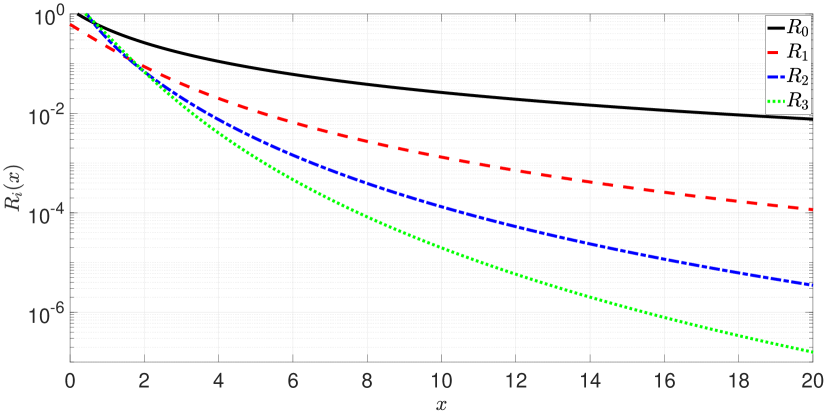
Figure 1: Rate of convergence for the upper and lower bounds on the right tail of the Gaussian RV with $\sigma=1.9$, $\mu=-1.7$.

In Fig. 1, we show the rate of convergence, given by (137), for $i=0,\;1,\;2,$ and $3$, of the upper and lower bounds on the right tail of the Gaussian RV with $\sigma=1.9$ and $\mu=-1.7$. Fig. 1 shows that the upper and lower bounds on the Gaussian tail converge to each other very fast. Specifically, $P_{0}(x)$ and $P_{1}(x)$ converge to each other with rate proportional to $1/x^{2}$, $P_{1}(x)$ and $P_{2}(x)$ converge to each other with rate proportional to $1/x^{4}$, $P_{2}(x)$ and $P_{3}(x)$ converge to each other with rate proportional to $1/x^{6}$, and $P_{3}(x)$ and $P_{4}(x)$ converge to each other with rate proportional to $1/x^{8}$.

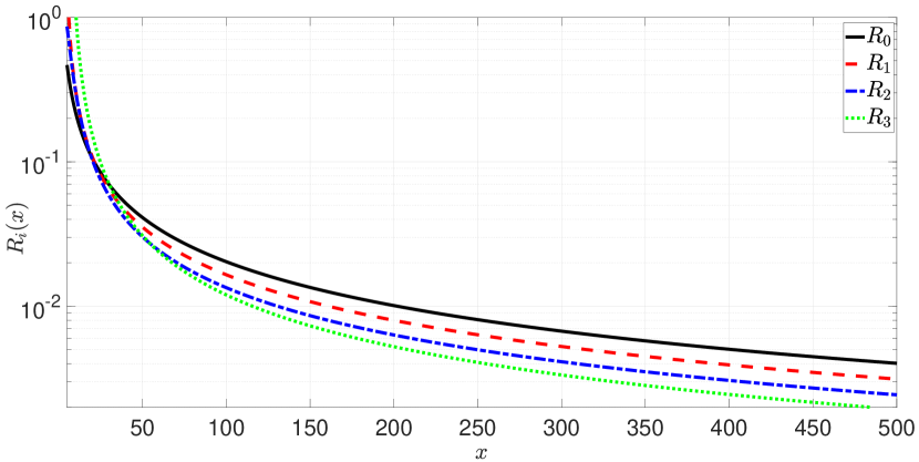
Figure 2: Rate of convergence for the upper and lower bounds on the right tail of the beta prime RV with $\alpha=2.1$, $\beta=1.3$.

For the beta prime right tail bounds, using the function $g_{X}(x)=xf_{X}(x)$ (note $l=0$) to construct the seed, we obtain the following expressions for the bounds

$$1-F_{X}(x)\leq P_{0}(x) =\frac{x^{\alpha}(x+1)^{-\alpha-\beta+1}}{B(\alpha,\beta)(\beta x-\alpha)},\;\forall x>\frac{\alpha}{\beta}$$ (145)

$$1-F_{X}(x)\geq P_{1}(x) =\frac{x^{\alpha}(x+1)^{-\alpha-\beta+1}(\beta x-\alpha)}{B(\alpha,\beta)\left(\alpha^{2}+\beta^{2}x^{2}+x(-2\alpha\beta+\alpha+\beta)\right)},\;\forall x>\frac{\alpha}{\beta},$$ (146)

$$1-F_{X}(x)\leq P_{2}(x)$$ , (147)

$$1-F_{X}(x)\geq P_{3}(x)$$ , (148)

$$1-F_{X}(x)\leq P_{4}(x)$$ . (149)

We also have expressions for $P_{2}(x)$, $P_{3}(x)$, and $P_{4}(x)$, which we use to plot $R_{1}(x)$, $R_{2}(x)$, and $R_{3}(x)$ in Fig. 2, but we omit to show them analytically since they are too large to be fit within one row.

In Fig. 2, we show the rate of convergence, given by (137), for $i=0,\;1,\;2,$ and $3$, of the upper and lower bounds on the right tail of the beta prime RV with $\alpha=2.1$ and $\beta=1.3$. Fig. 2 shows that the upper and lower bounds on the right tail of the beta prime RV, specifically, the pairs $P_{0}(x)$ and $P_{1}(x)$, $P_{1}(x)$ and $P_{2}(x)$, $P_{2}(x)$ and $P_{3}(x)$, and $P_{3}(x)$ and $P_{4}(x)$ converge to each other with rate proportional to $1/x$.

VIII-B The Left Tail

For the left tail, we also use the iterative method to obtain ever tighter lower and upper bounds. To this end, for constructing the seed, $P_{0}(x)$, we will use $g_{X}(x)=(x-l)f_{X}(x)$ for the non-central chi-squared RV (note $l=0$).

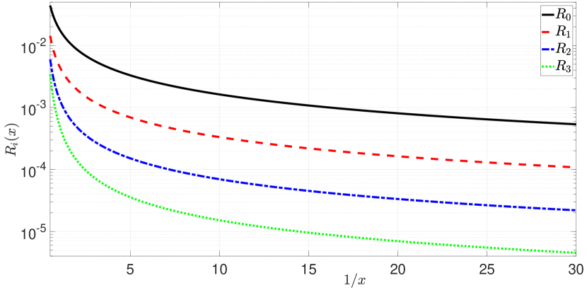
Figure 3: Rate of convergence for the upper and lower bounds on the left tail for the non-central chi-squared RV with $k=10$, $\lambda=2$.

For the left tail bounds of the non-central chi-squared RV, using the function $g_{X}(x)=xf_{X}(x)$ to construct the seed, we obtain the following expressions

$$F_{X}(x)\leq P_{0}(x) =\frac{e^{\frac{1}{2}(-\lambda-x)}\sqrt{\lambda x}\left(\frac{x}{\lambda}\right)^{k/4}I_{\frac{k-2}{2}}\left(\sqrt{x\lambda}\right){}^{2}}{(k-x-2)I_{\frac{k-2}{2}}\left(\sqrt{x\lambda}\right)+\sqrt{\lambda x}I_{\frac{k}{2}}\left(\sqrt{x\lambda}\right)},\;\forall x<k-2,$$ (150)

$$F_{X}(x)\geq P_{1}(x)$$ , (151)

$$F_{X}(x)\leq P_{2}(x)$$ , (152)

$$F_{X}(x)\geq P_{3}(x)$$ , (153)

$$F_{X}(x)\leq P_{4}(x)$$ . (154)

We also have expressions for $P_{1}(x)$, $P_{2}(x)$, $P_{3}(x)$, and $P_{4}(x)$, which we use to plot $R_{1}(x)$, $R_{2}(x)$, and $R_{3}(x)$ in Fig. 3, but we omit to show them analytically since they are too large to be fit in one row.

In Fig. 3, we show the rate of convergence, given by (137), for $i=0,\;1,\;2,$ and $3$, of the upper and lower bounds on the left tail of the non-central chi-squared RV with $k=10$ and $\lambda=2$. Fig. 3 shows that the upper and lower bounds on the left tail of the non-central chi-squared RV, specifically, the pairs $P_{0}(x)$ and $P_{1}(x)$, $P_{1}(x)$ and $P_{2}(x)$, $P_{2}(x)$ and $P_{3}(x)$, and $P_{3}(x)$ and $P_{4}(x)$ converge to each other with rate proportional to $x$, as $x\to 0$.

We note that the bounds $P_{0}(x)$ and $P_{1}(x)$ on the left tail of the non-central chi-squared RV might be useful for a better understanding of Polyanskiy-Poor-Verdú converse bound for the finite blocklength AWGN channel, since this converse bound is given in the form of the left tail of the non-central chi-squared distribution, see [13]. To this end, we may use simple bounds on the modified Bessel function of the first kind, which is present in these bounds, see e.g. (150). This possible research direction is left for future works.

IX Conclusion

We provided a general method for upper and lower bounding both the left and the right tail probabilities of continuous random variables. The proposed method requires setting a function $g_{X}(x)$ with certain conditions, which if satisfied, results in upper and lower bounds that are functions of $g_{X}(x)$, $g^{\prime}_{X}(x)$, and the PDF of $X$, $f_{X}(x)$. We also proposed an iterative method that results in ever tighter upper and lower bounds on the tails, under certain conditions. Finally, we established connections between the proposed bounds and Markov’s inequality and Chernoff’s bound.

Finally, the method used for proving the upper and lower bounds on $1-F_{X}(x)$ and on $F_{X}(x)$ relies on the fact that the values of $1-F_{X}(x)$ and $F_{X}(x)$ are known to be zero at $x=r$ and $x=l$, respectively. In general, there is nothing special about these values, and the method can be applied in a similar fashion if other values of $F_{X}(x)$ (i.e., $1-F_{X}(x)$) are known. Finally, there is nothing special about $F_{X}(x)$, which is an integral of $f_{X}(x)$, and the method can be applied in a similar fashion for upper bounding and lower bounding other integrals as well, if these integrals are known for some points (i.e., integration limits). We leave this research direction for future works.

-A Proof Of Lemma 1

If

$$\frac{1-F_{X}(x)}{g_{X}(x)}$$ (155)

is a deceasing function on the interval $I$, then the following holds

$$\diff{}{x}\left(\frac{1-F_{X}(x)}{g_{X}(x)}\right)\leq 0,\;\forall x\in I.$$ (156)

By expanding the derivative in (156), we obtain

$$\frac{-f_{X}(x)}{g_{X}(x)}-\frac{\big{(}1-F_{X}(x)\big{)}g^{\prime}_{X}(x)}{g^{2}_{X}(x)}\leq 0,\;\forall x\in I.$$ (157)

Multiplying both sides of (157) by $g^{2}_{X}(x)$, we obtain

$$-f_{X}(x)g_{X}(x)-\big{(}1-F_{X}(x)\big{)}g^{\prime}_{X}(x)\leq 0,\;\forall x\in I.$$ (158)

Now dividing both sides by $g^{\prime}_{X}(x)$, and taking into account that $g^{\prime}_{X}(x)<0$, we obtain

$$-f_{X}(x)\frac{g_{X}(x)}{g^{\prime}_{X}(x)}-\big{(}1-F_{X}(x)\big{)}\geq 0,\;\forall x\in I.$$ (159)

Rearranging (159), we obtain the desired result in (8).

On the other hand, if

$$\diff{}{x}\left(\frac{1-F_{X}(x)}{g_{X}(x)}\right)\geq 0,\;\forall x\in I,$$ (160)

then following the same procedure as above leads to the desired result in (11). This completes the proof.

-B Proof Of Theorem 1

We start with the bound given by (8) in Lemma 1, which for $I=[\hat{x}_{0},r]$, can be equivalently written as

$$1-F_{X}(x)+f_{X}(x)\frac{g_{X}(x)}{g^{\prime}_{X}(x)}\leq 0,\;\forall x>\hat{x}_{0}.$$ (161)

As stated in Lemma 1, the bound in (161) holds if $g_{X}(x)$ is continuous, $g_{X}(x)>0$, and $g^{\prime}_{X}(x)<0$, $\forall x>\hat{x}_{0}$. Now let us define a function $D_{X}(x)$ that is equal to the left-hand side of (161), and thereby given by

$$D_{X}(x)=1-F_{X}(x)+f_{X}(x)\frac{g_{X}(x)}{g^{\prime}_{X}(x)}.$$ (162)

First note the following obvious property: If a function $G(x)$ is an increasing function for $x_{0}<x<r$ and if $G(x)$ converges to $\lim\limits_{x\to r}G(x)=0$, then the function $G(x)$ must be a non-positive function for $x_{0}<x\leq r$, i.e., $G(x)\leq 0$ for $x_{0}<x\leq r$.

We now use this property for the construction of this proof. Specifically, in the following, we investigate the properties that $g_{X}(x)$ must satisfy in order for $D_{X}(x)$, given by (162), to satisfy $i)$ $\lim\limits_{x\to r}D_{X}(x)=0$ and $ii)$ $D_{X}(x)$ to be an increasing function $\forall x>x_{0}$, since then $D_{X}(x)\leq 0$, $\forall x>x_{0}$ holds, as per the property described above. On the other hand, when $D_{X}(x)\leq 0$, $\forall x>x_{0}$ holds, then the upper bound in (16) holds, and thereby we have obtained our proof for the upper bound in (16).

We start with investigating the conditions of $g_{X}(x)$ for which $i)$ $\lim\limits_{x\to r}D_{X}(x)=0$ holds. Now, for $D_{X}(x)$ given by (162), condition $\lim\limits_{x\to r}D_{X}(x)=0$ is always met since this theorem assumes that (13) holds. Specifically, we have

$$\lim\limits_{x\to r}D_{X}(x) =\lim\limits_{x\to r}\big{(}1-F_{X}(x)\big{)}+\lim_{x\to r}f_{X}(x)\frac{g_{X}(x)}{g^{\prime}_{X}(x)}=\lim_{x\to r}f_{X}(x)\frac{g_{X}(x)}{g^{\prime}_{X}(x)}\stackrel{{\scriptstyle(a)}}{{=}}0,$$ (163)

where $(a)$ follows from the assumption in this theorem that $g_{X}(x)$ is such that condition (13) is satisfied.

We now continue investigating the conditions of $g_{X}(x)$ that make $ii)$ $D_{X}(x)$ to be an increasing function $\forall x>x_{0}$. For $D_{X}(x)$ to be an increasing function $\forall x>x_{0}$, then the following must hold

$$\diff{}{x}D_{X}(x)\geq 0,\;\forall x>x_{0}.$$ (164)

Inserting $D_{X}(x)$ from (162) into (164) and carrying out the derivative, we obtain

$$-f_{X}(x)+f^{\prime}_{X}(x)\frac{g_{X}(x)}{g^{\prime}_{X}(x)}+f_{X}(x)\left(\frac{g^{\prime}_{X}(x)}{g^{\prime}_{X}(x)}-\frac{g_{X}(x)g^{\prime\prime}_{X}(x)}{\big{(}g^{\prime}_{X}(x)\big{)}^{2}}\right)\geq 0,\;\forall x>x_{0},$$ (165)

which is equivalent to

$$-f_{X}(x)+f^{\prime}_{X}(x)\frac{g_{X}(x)}{g^{\prime}_{X}(x)}+f_{X}(x)-f_{X}(x)\frac{g_{X}(x)g^{\prime\prime}_{X}(x)}{\big{(}g^{\prime}_{X}(x)\big{)}^{2}}\geq 0,\;\forall x>x_{0},$$ (166)

which is equivalent to

$$f^{\prime}_{X}(x)\frac{g_{X}(x)}{g^{\prime}_{X}(x)}-f_{X}(x)\frac{g_{X}(x)g^{\prime\prime}_{X}(x)}{\big{(}g^{\prime}_{X}(x)\big{)}^{2}}\geq 0,\;\forall x>x_{0}.$$ (167)

Multiplying both sides of (167) by $\frac{g_{X}(x)}{g^{\prime}_{X}(x)}$, and taking into consideration that $\frac{g_{X}(x)}{g^{\prime}_{X}(x)}<0$, $\forall x>x_{0}$, we obtain the following equivalent inequality

$$f^{\prime}_{X}(x)-f_{X}(x)\frac{g^{\prime\prime}_{X}(x)}{g^{\prime}_{X}(x)}\leq 0,\;\forall x>x_{0}.$$ (168)

Dividing both sides of (168) by $f_{X}(x)$, we obtain the following equivalent inequality

$$\frac{f^{\prime}_{X}(x)}{f_{X}(x)}-\frac{g^{\prime\prime}_{X}(x)}{g^{\prime}_{X}(x)}\leq 0,\;\forall x>x_{0},$$ (169)

which is equivalent to

$$\ln^{\prime}\big{(}f_{X}(x)\big{)}-\ln^{\prime}\big{(}g^{\prime}_{X}(x)\big{)}\leq 0,\;\forall x>x_{0},$$ (170)

which is equivalent to

$$\ln^{\prime}\left(\frac{f_{X}(x)}{g^{\prime}_{X}(x)}\right)\leq 0,\;\forall x>x_{0},$$ (171)

and also to

$$\ln^{\prime}\left(\frac{f_{X}(x)}{-g^{\prime}_{X}(x)}\right)\leq 0,\;\forall x>x_{0}.$$ (172)

The expression (172) tells us that $D_{X}(x)$ is an increasing function $\forall x>x_{0}$, if the function

$$\ln\left(\frac{f_{X}(x)}{-g^{\prime}_{X}(x)}\right)$$ (173)

is a decreasing function, $\forall x>x_{0}$. Now since $\ln(\cdot)$ is a one-to-one function, (173) is a decreasing function when

$$\frac{f_{X}(x)}{-g^{\prime}_{X}(x)}$$ (174)

is a decreasing function $\forall x>x_{0}$. We now simplify the condition that (174) is decreasing function $\forall x>x_{0}$ as follows. The function in (174) is a deceasing function $\forall x>x_{0}$ if

$$\diff{}{x}\left(\frac{f_{X}(x)}{-g^{\prime}_{X}(x)}\right)\leq 0,\;\forall x>x_{0}.$$ (175)

On the other hand, the left-hand side of (175) can be written equivalently as

$$\diff{}{x}\left(\frac{f_{X}(x)}{-g^{\prime}_{X}(x)}\right) =\diff{}{x}\left(\frac{f_{X}(x)g_{X}(x)}{-g^{\prime}_{X}(x)g_{X}(x)}\right)=\diff{}{x}\left(\frac{P_{X}(x)}{g_{X}(x)}\right)=\frac{P^{\prime}_{X}(x)}{g_{X}(x)}-\frac{P_{X}(x)g^{\prime}_{X}(x)}{g^{2}_{X}(x)}$$

$$=\frac{P^{\prime}_{X}(x)}{g_{X}(x)}-\frac{P_{X}(x)g^{\prime}_{X}(x)f_{X}(x)}{g^{2}_{X}(x)f_{X}(x)}=\frac{P^{\prime}_{X}(x)}{g_{X}(x)}+\frac{P_{X}(x)f_{X}(x)}{P_{X}(x)g_{X}(x)}=\frac{P^{\prime}_{X}(x)}{g_{X}(x)}+\frac{f_{X}(x)}{g_{X}(x)}.$$ (176)

Inserting (-B) into (175) and multiplying both sides of the inequality by $g_{X}(x)$, we obtain

$$P^{\prime}_{X}(x)+f_{X}(x)\leq 0,\;\forall x>x_{0}.$$ (177)

Therefore, if (177) holds $\forall x>x_{0}$ and since (163) always holds, then

$$D_{X}(x)\leq 0,\;\forall x>x_{0}.$$ (178)

Inserting (162) into (178), we obtain (16), which is the first bound we aimed to prove.

For the second bound in this theorem, we follow the same method as above. To this end, we use the following obvious property: If a function $G(x)$ is a decreasing function for $x_{0}<x<r$ and if $G(x)$ converges to $\lim\limits_{x\to r}G(x)=0$, then the function $G(x)$ must be a non-negative function for $x_{0}<x\leq r$, i.e., $G(x)\geq 0$ for $x_{0}<x\leq r$. Thereby, it is straightforward to prove that $D_{X}(x)\geq 0$ if

$$\frac{f_{X}(x)}{-g^{\prime}_{X}(x)}$$ (179)

is an increasing function $\forall x>x_{0}$. Taking into account the proof of the first bound, the proof of the second bound is omitted due to its redundancy. This concludes the proof of this theorem.

-C Proof Of Lemma 2

Since $\lim\limits_{x\to r}g_{X}(x)=0$ holds, we have the following limit for $P_{X}(x)$

$$\lim_{x\to r}P_{X}(x) =\lim_{x\to r}-f_{X}(x)\frac{g_{X}(x)}{g^{\prime}_{X}(x)}=\lim_{x\to r}g_{X}(x)\lim_{x\to r}\frac{-f_{X}(x)}{g^{\prime}_{X}(x)}\stackrel{{\scriptstyle(a)}}{{=}}\lim_{x\to r}g_{X}(x)\lim_{x\to r}\frac{1-F_{X}(x)}{g_{X}(x)}$$

$$=\lim_{x\to r}g_{X}(x)\frac{1-F_{X}(x)}{g_{X}(x)}=\lim_{x\to r}\big{(}1-F_{X}(x)\big{)}=0,$$ (180)

where $(a)$ follows from (reverse) l’Hopital’s rule, which is valid since $1-F_{X}(x)$ and $g_{X}(x)$ both tend to $0$ as $x\to r$.

-D Proof Of Lemma 3

Since we assume that (64) is valid upper bound or a valid lower bound, $\forall x>x_{0}$, as per Theorem 1, then $\lim\limits_{x\to r}P_{0}(x)=0$ must hold. Now, if $\lim\limits_{x\to r}P_{0}(x)=0$ holds, then the next iteration, $P_{1}(x)$, obtained by setting $i=0$ in (65), must satisfy

$$\lim\limits_{x\to r}P_{1}(x)=0,$$ (181)

according to Lemma 2. Now, since (181) holds, then $P_{2}(x)$, obtained by setting $i=1$ in (65) must also satisfy

$$\lim\limits_{x\to r}P_{2}(x)=0,$$ (182)

according to Lemma 2. These true statements can be extended to any $i+1$, thereby proving that (66) holds.

-E Proof Of Lemma 4

Let $P_{i}$ be an upper bound on $1-F_{X}(x)$, $\forall x>x_{0}$, as per Theorem 1. Then, according to (15), the following holds

$$P^{\prime}_{i}(x)\leq-f_{X}(x),\;\forall x>x_{0},$$ (183)

which is equivalent to

$$1\geq-f_{X}(x)\frac{1}{P^{\prime}_{i}(x)},\;\forall x>x_{i},$$ (184)

and is obtained by dividing both sides of (184) by $P^{\prime}_{i}(x)<0$, which is a valid division only for $x>\hat{x}$, due to the assumption $P^{\prime}_{i}(x)<0$, $x>\hat{x}$. Now, (184) is equivalent to

$$1\geq-f_{X}(x)\frac{P_{i}(x)}{P^{\prime}_{i}(x)}\frac{1}{P_{i}(x)},\;\forall x>x_{i},$$ (185)

which is equivalent to

$$1\geq\frac{P_{i+1}(x)}{P_{i}(x)},\;\forall x>x_{i},$$ (186)

which is equivalent to

$$P_{i}(x)\geq P_{i+1}(x),\;\forall x>x_{i},$$ (187)

which is the result in (67) that we aimed to prove.

We now prove (68). Let $P_{i}$ be a lower bound on $1-F_{X}(x)$, $\forall x>x_{0}$, as per Theorem 1. Then, according to (18), the following holds

$$P^{\prime}_{i}(x)\geq-f_{X}(x),\;\forall x>x_{0},$$ (188)

which is equivalent to

$$1\leq-f_{X}(x)\frac{1}{P^{\prime}_{i}(x)},\;\forall x>x_{i},$$ (189)

and is obtained by dividing both sides of (189) by $P^{\prime}_{i}(x)<0$, which is a valid division only for $x>\hat{x}$. Now, (189) is equivalent to

$$1\leq-f_{X}(x)\frac{P_{i}(x)}{P^{\prime}_{i}(x)}\frac{1}{P_{i}(x)},\;\forall x>x_{i},$$ (190)

which is equivalent to

$$1\leq\frac{P_{i+1}(x)}{P_{i}(x)},\;\forall x>x_{i},$$ (191)

which is equivalent to

$$P_{i}(x)\leq P_{i+1}(x),\;\forall x>x_{i},$$ (192)

which is the result in (68) that we aimed to prove.

-F Proof Of Lemma 5

We start with the first part of this lemma when $P_{i}(x)$ and $P_{i+1}(x)$ are both valid upper and lower bounds on $1-F_{X}(x)$, $\forall x>x_{i+1}$, respectively, as per Theorem 1.

First, note that from (69), that the following holds

$$\frac{P_{L,i}(x)+P_{i}(x)}{2}=1-F_{X}(x),\;\forall x>x_{i+1}.$$ (193)

Then, if $P_{L,i}(x)\leq P_{i+1}(x)$ holds, from (193), we obtain that the following must hold

$$\frac{P_{i+1}(x)+P_{i}(x)}{2}\geq 1-F_{X}(x),\;\forall x>x_{i+1},$$ (194)

which means that $\frac{P_{i+1}(x)+P_{i}(x)}{2}$ is an upper bound on $1-F_{X}(x)$, $\forall x>x_{i+1}$. Now, according to Theorem 1, in order for $\frac{P_{i+1}(x)+P_{i}(x)}{2}$ to be an upper bound on $1-F_{X}(x)$, $\forall x>x_{i+1}$, i.e., (194) to hold, the following must hold

$$\frac{P^{\prime}_{i+1}(x)+P^{\prime}_{i}(x)}{2}+f_{X}(x)\leq 0,\;\forall x>x_{i+1},$$ (195)

which is equivalent to

$$P^{\prime}_{i+1}(x)+P^{\prime}_{i}(x)+2f_{X}(x)\leq 0,\;\forall x>x_{i+1}.$$ (196)

Going now in reverse order, it is straightforward to obtain that if (196) holds, then $P_{L,i}(x)\leq P_{i+1}(x)$ also holds. This completes the first part of this lemma.

We now prove the second part of this lemma when $P_{i}(x)$ and $P_{i+1}(x)$ are both valid lower and upper bounds on $1-F_{X}(x)$, $\forall x>x_{i+1}$, respectively, as per Theorem 1.

First, note that from (70), that the following holds

$$\frac{P_{U,i}(x)+P_{i}(x)}{2}=1-F_{X}(x),\;\forall x>x_{i+1}.$$ (197)

Then, if $P_{U,i}(x)\geq P_{i+1}(x)$ holds, from (197), we obtain that the following must hold

$$\frac{P_{i+1}(x)+P_{i}(x)}{2}\leq 1-F_{X}(x),\;\forall x>x_{i+1},$$ (198)

which means that $\frac{P_{i+1}(x)+P_{i}(x)}{2}$ is a lower bound on $1-F_{X}(x)$, $\forall x>x_{i+1}$. Now, according to Theorem 1, in order for $\frac{P_{i+1}(x)+P_{i}(x)}{2}$ to be an lower bound on $1-F_{X}(x)$, $\forall x>x_{i+1}$, i.e., (198) to hold, the following must hold

$$\frac{P^{\prime}_{i+1}(x)+P^{\prime}_{i}(x)}{2}+f_{X}(x)\geq 0,\;\forall x>x_{i+1},$$ (199)

which is equivalent to

$$P^{\prime}_{i+1}(x)+P^{\prime}_{i}(x)+2f_{X}(x)\geq 0,\;\forall x>x_{i+1}.$$ (200)

Going now in reverse order, it is straightforward to obtain that if (200) holds, then $P_{U,i}(x)\geq P_{i+1}(x)$ also holds. This completes the second part of this lemma.

Finally, note that we have used Theorem 1 for determining whether $\frac{P_{i+1}(x)+P_{i}(x)}{2}$ is an upper bound or a lower bound, as per Theorem 1, and this is valid since

$$\lim_{x\to r}\frac{P_{i+1}(x)+P_{i}(x)}{2}=0$$ (201)

holds due to Lemma 3. This completes the proof of this lemma.

-G Proof Of Theorem 2

We aim to prove

$$F_{X}(x)\leq f_{X}(x)\frac{g_{X}(x)}{g^{\prime}_{X}(x)},\;\forall x<x_{0},$$ (202)

which is equivalent to

$$F_{X}(x)-f_{X}(x)\frac{g_{X}(x)}{g^{\prime}_{X}(x)}\leq 0,\;\forall x<x_{0}.$$ (203)

Now let us again define a function $D_{X}(x)$ that is equal to the left-hand side of (203), and thereby given by

$$D_{X}(x)=F_{X}(x)-f_{X}(x)\frac{g_{X}(x)}{g^{\prime}_{X}(x)}.$$ (204)

Note now the following obvious property: If a function $G(x)$ is a decreasing function for $l<x<x_{0}$ and if $G(x)$ converges to $\lim\limits_{x\to l}G(x)=0$, then the function $G(x)$ must be a non-positive function for $l<x\leq x_{0}$, i.e., $G(x)\leq 0$ for $l<x\leq x_{0}$.

We now use this property for the construction of this proof. Specifically, in the following, we investigate the properties that $g_{X}(x)$ must satisfy in order for $D_{X}(x)$, given by (204), to satisfy $i)$ $\lim\limits_{x\to l}D_{X}(x)=0$ and $ii)$ $D_{X}(x)$ to be a decreasing function $\forall x<x_{0}$, since then $D_{X}(x)\leq 0$, $\forall x<x_{0}$ holds, according to property described above. On the other hand, when $D_{X}(x)\leq 0$, $\forall x<x_{0}$, holds, then the upper bound in (84) holds, and thereby we have obtained our proof for the upper bound in (84).

We start with investigating the conditions of $g_{X}(x)$ for which $i)$ $\lim\limits_{x\to l}D_{X}(x)=0$ holds. Now, for $D_{X}(x)$ given by (204), condition $\lim\limits_{x\to l}D_{X}(x)=0$ is always met since this theorem assumes that (81) holds. Specifically, we have

$$\lim\limits_{x\to l}D_{X}(x) =\lim\limits_{x\to l}F_{X}(x)-\lim_{x\to l}f_{X}(x)\frac{g_{X}(x)}{g^{\prime}_{X}(x)}=-\lim_{x\to l}f_{X}(x)\frac{g_{X}(x)}{g^{\prime}_{X}(x)}\stackrel{{\scriptstyle(a)}}{{=}}0,$$ (205)

where $(a)$ follows from the assumption in this theorem that $g_{X}(x)$ is such that condition (81) is satisfied.

We now continue investigating the conditions of $g_{X}(x)$ that make $ii)$ $D_{X}(x)$ to be a decreasing function $\forall x<x_{0}$. For $D_{X}(x)$ to be a decreasing function $\forall x<x_{0}$, the following must hold

$$\diff{}{x}D_{X}(x)\leq 0,\;\forall x<x_{0}.$$ (206)

Inserting $D_{X}(x)$ from (204) into (206) and carrying out the derivative, we obtain

$$f_{X}(x)-f^{\prime}_{X}(x)\frac{g_{X}(x)}{g^{\prime}_{X}(x)}-f_{X}(x)\left(\frac{g^{\prime}_{X}(x)}{g^{\prime}_{X}(x)}-\frac{g_{X}(x)g^{\prime\prime}_{X}(x)}{\big{(}g^{\prime}_{X}(x)\big{)}^{2}}\right)\leq 0,\;\forall x<x_{0},$$ (207)

which is equivalent to

$$f_{X}(x)-f^{\prime}_{X}(x)\frac{g_{X}(x)}{g^{\prime}_{X}(x)}-f_{X}(x)+f_{X}(x)\frac{g_{X}(x)g^{\prime\prime}_{X}(x)}{\big{(}g^{\prime}_{X}(x)\big{)}^{2}}\leq 0,\;\forall x<x_{0},$$ (208)

which is equivalent to

$$-f^{\prime}_{X}(x)\frac{g_{X}(x)}{g^{\prime}_{X}(x)}+f_{X}(x)\frac{g_{X}(x)g^{\prime\prime}_{X}(x)}{\big{(}g^{\prime}_{X}(x)\big{)}^{2}}\leq 0,\;\forall x<x_{0}.$$ (209)

Multiplying both sides of (209) by $-\frac{g_{X}(x)}{g^{\prime}_{X}(x)}$, and taking into consideration that $-\frac{g_{X}(x)}{g^{\prime}_{X}(x)}<0$, $\forall x<x_{0}$, we obtain the following equivalent inequality

$$f^{\prime}_{X}(x)-f_{X}(x)\frac{g^{\prime\prime}_{X}(x)}{g^{\prime}_{X}(x)}\geq 0,\;\forall x<x_{0}.$$ (210)

Dividing both sides of (210) by $f_{X}(x)$, we obtain the following equivalent inequality

$$\frac{f^{\prime}_{X}(x)}{f_{X}(x)}-\frac{g^{\prime\prime}_{X}(x)}{g^{\prime}_{X}(x)}\geq 0,\;\forall x<x_{0},$$ (211)

which is equivalent to

$$\ln^{\prime}\big{(}f_{X}(x)\big{)}-\ln^{\prime}\big{(}g^{\prime}_{X}(x)\big{)}\geq 0,\;\forall x<x_{0},$$ (212)

which is equivalent to

$$\ln^{\prime}\left(\frac{f_{X}(x)}{g^{\prime}_{X}(x)}\right)\geq 0,\;\forall x<x_{0},$$ (213)

and also to

$$\ln^{\prime}\left(\frac{f_{X}(x)}{-g^{\prime}_{X}(x)}\right)\geq 0,\;\forall x<x_{0}.$$ (214)

The expression (213) tells us that $D_{X}(x)$ is a decreasing function $\forall x<x_{0}$ if the function

$$\ln\left(\frac{f_{X}(x)}{g^{\prime}_{X}(x)}\right)$$ (215)

is an increasing function, $\forall x<x_{0}$. Now since $\ln(\cdot)$ is a one-to-one function, (215) is an increasing function when

$$\frac{f_{X}(x)}{g^{\prime}_{X}(x)}$$ (216)

is an increasing function $\forall x<x_{0}$. We now simplify the condition that (216) is an increasing function $\forall x<x_{0}$ as follows. The function in (216) is an increasing function $\forall x<x_{0}$ if

$$\diff{}{x}\left(\frac{f_{X}(x)}{g^{\prime}_{X}(x)}\right)\geq 0,\;\forall x<x_{0}.$$ (217)

On the other hand, the left-hand side of (217) can be written equivalently as

$$\diff{}{x}\left(\frac{f_{X}(x)}{g^{\prime}_{X}(x)}\right) =\diff{}{x}\left(\frac{f_{X}(x)g_{X}(x)}{g^{\prime}_{X}(x)g_{X}(x)}\right)=\diff{}{x}\left(\frac{P_{X}(x)}{g_{X}(x)}\right)=\frac{P^{\prime}_{X}(x)}{g_{X}(x)}-\frac{P_{X}(x)g^{\prime}_{X}(x)}{g^{2}_{X}(x)}$$

$$=\frac{P^{\prime}_{X}(x)}{g_{X}(x)}-\frac{P_{X}(x)g^{\prime}_{X}(x)f_{X}(x)}{g^{2}_{X}(x)f_{X}(x)}=\frac{P^{\prime}_{X}(x)}{g_{X}(x)}-\frac{P_{X}(x)f_{X}(x)}{P_{X}(x)g_{X}(x)}=\frac{P^{\prime}_{X}(x)}{g_{X}(x)}-\frac{f_{X}(x)}{g_{X}(x)}.$$ (218)

Inserting (-G) into (217) and multiplying both sides of the inequality by $g_{X}(x)$, we obtain

$$P^{\prime}_{X}(x)-f_{X}(x)\geq 0,\;\forall x<x_{0}.$$ (219)

Therefore, if (219) holds $\forall x<x_{0}$ and since (205) always holds, then

$$D_{X}(x)\leq 0,\;\forall x<x_{0}.$$ (220)

Inserting (204) into (220), we obtain (84), which is the first bound we aimed to prove.

For the second bound in this Theorem, we follow the same method as above. This this end, we use the following obvious property: If a function $G(x)$ is an increasing function for $l<x<x_{0}$ and if $G(x)$ converges to $\lim\limits_{x\to l}G(x)=0$, then the function $G(x)$ must be a non-negative function for $l<x\leq x_{0}$, , i.e., $G(x)\geq 0$ for $l<x\leq x_{0}$. Thereby, it is straightforward to prove that $D_{X}(x)\geq 0$ if

$$\frac{f_{X}(x)}{g^{\prime}_{X}(x)}$$ (221)

is a decreasing function $\forall x<x_{0}$. Taking into account the proof of the first bound, the proof of the second bound is omitted due to its redundancy. This concludes the proof of this theorem.

-H Proof Of Lemma 6

Since $\lim\limits_{x\to l}g_{X}(x)=0$ holds, we have the following limit for $P_{X}(x)$

$$\lim_{x\to l}P_{X}(x) =\lim_{x\to l}f_{X}(x)\frac{g_{X}(x)}{g^{\prime}_{X}(x)}=\lim_{x\to l}g_{X}(x)\lim_{x\to l}\frac{f_{X}(x)}{g^{\prime}_{X}(x)}\stackrel{{\scriptstyle(a)}}{{=}}\lim_{x\to l}g_{X}(x)\lim_{x\to l}\frac{F_{X}(x)}{g_{X}(x)}$$

$$=\lim_{x\to l}g_{X}(x)\frac{F_{X}(x)}{g_{X}(x)}=\lim_{x\to l}F_{X}(x)=0,$$ (222)

where $(a)$ follows from (reverse) l’Hopital’s rule, which is valid since $F_{X}(x)$ and $g_{X}(x)$ both tend to $0$ as $x\to l$.

-I Proof Of Lemma 7

Since we assume that (114) is valid upper bound or a valid lower bound, $\forall x<x_{0}$, as per Theorem 2, then $\lim\limits_{x\to l}P_{0}(x)=0$ must hold. Now, if $\lim\limits_{x\to l}P_{0}(x)=0$ holds, then the next iteration, $P_{1}(x)$, obtained by setting $i=0$ in (115), must satisfy

$$\lim\limits_{x\to l}P_{1}(x)=0,$$ (223)

according to Lemma 6. Now, since (223) holds, then $P_{2}(x)$, obtained by setting $i=1$ in (115) must also satisfy

$$\lim\limits_{x\to l}P_{2}(x)=0,$$ (224)

according to Lemma 6. These true statements can be extended to any $i+1$, thereby proving that (116) holds.

-J Proof Of Lemma 8

Let $P_{i}$ be an upper bound on $F_{X}(x)$, $\forall x<x_{0}$, as per Theorem 2. Then, according to (83), the following holds

$$P^{\prime}_{i}(x)\geq f_{X}(x),\;\forall x<x_{0},$$ (225)

which is equivalent to

$$1\geq f_{X}(x)\frac{1}{P^{\prime}_{i}(x)},\;\forall x<x_{i},$$ (226)

and is obtained by dividing both sides of (226) by $P^{\prime}_{i}(x)>0$, which is a valid division only for $x<\hat{x}$, due to the assumption $P^{\prime}_{i}(x)>0$, $x<\hat{x}$. Now, (226) is equivalent to

$$1\geq f_{X}(x)\frac{P_{i}(x)}{P^{\prime}_{i}(x)}\frac{1}{P_{i}(x)},\;\forall x<x_{i},$$ (227)

which is equivalent to

$$1\geq\frac{P_{i+1}(x)}{P_{i}(x)},\;\forall x<x_{i},$$ (228)

which is equivalent to

$$P_{i}(x)\geq P_{i+1}(x),\;\forall x<x_{i},$$ (229)

which is the result in (117) that we aimed to prove.

We now prove (118). Let $P_{i}$ be a lower bound on $F_{X}(x)$, $\forall x<x_{0}$, as per Theorem 2. Then, according to (86), the following holds

$$P^{\prime}_{i}(x)\leq f_{X}(x),\;\forall x<x_{0},$$ (230)

which is equivalent to

$$1\leq f_{X}(x)\frac{1}{P^{\prime}_{i}(x)},\;\forall x<x_{i},$$ (231)

and is obtained by dividing both sides of (231) by $P^{\prime}_{i}(x)>0$, which is a valid division only for $x<\hat{x}$. Now, (231) is equivalent to

$$1\leq f_{X}(x)\frac{P_{i}(x)}{P^{\prime}_{i}(x)}\frac{1}{P_{i}(x)},\;\forall x<x_{i},$$ (232)

which is equivalent to

$$1\leq\frac{P_{i+1}(x)}{P_{i}(x)},\;\forall x<x_{i},$$ (233)

which is equivalent to

$$P_{i}(x)\leq P_{i+1}(x),\;\forall x<x_{i},$$ (234)

which is the result in (118) that we aimed to prove.

-K Proof Of Lemma 9

We start with the first part of this lemma when $P_{i}(x)$ and $P_{i+1}(x)$ are both valid upper and lower bounds on $F_{X}(x)$, $\forall x<x_{i+1}$, respectively, as per Theorem 2.

First, note that from (119), that the following holds

$$\frac{P_{L,i}(x)+P_{i}(x)}{2}=F_{X}(x),\;\forall x<x_{i+1}.$$ (235)

Then, if $P_{L,i}(x)\leq P_{i+1}(x)$ holds, from (235), we obtain that the following must hold

$$\frac{P_{i+1}(x)+P_{i}(x)}{2}\geq F_{X}(x),\;\forall x<x_{i+1},$$ (236)

which means that $\frac{P_{i+1}(x)+P_{i}(x)}{2}$ is an upper bound on $F_{X}(x)$, $\forall x<x_{i+1}$. Now, according to Theorem 2, in order for $\frac{P_{i+1}(x)+P_{i}(x)}{2}$ to be an upper bound on $F_{X}(x)$, $\forall x<x_{i+1}$, i.e., (236) to hold, the following must hold

$$\frac{P^{\prime}_{i+1}(x)+P^{\prime}_{i}(x)}{2}-f_{X}(x)\geq 0,\;\forall x<x_{i+1},$$ (237)

which is equivalent to

$$P^{\prime}_{i+1}(x)+P^{\prime}_{i}(x)-2f_{X}(x)\geq 0,\;\forall x<x_{i+1}.$$ (238)

Going now in reverse order, it is straightforward to obtain that if (238) holds, then $P_{L,i}(x)\leq P_{i+1}(x)$ also holds. This completes the first part of this lemma.

We now prove the second part of this lemma when $P_{i}(x)$ and $P_{i+1}(x)$ are both valid lower and upper bounds on $F_{X}(x)$, $\forall x<x_{i+1}$, respectively, as per Theorem 2.

First, note that from (120), that the following holds

$$\frac{P_{U,i}(x)+P_{i}(x)}{2}=F_{X}(x),\;\forall x<x_{i+1}.$$ (239)

Then, if $P_{U,i}(x)\geq P_{i+1}(x)$ holds, from (239), we obtain that the following must hold

$$\frac{P_{i+1}(x)+P_{i}(x)}{2}\leq F_{X}(x),\;\forall x<x_{i+1},$$ (240)

which means that $\frac{P_{i+1}(x)+P_{i}(x)}{2}$ is a lower bound on $F_{X}(x)$, $\forall x<x_{i+1}$. Now, according to Theorem 2, in order for $\frac{P_{i+1}(x)+P_{i}(x)}{2}$ to be an lower bound on $F_{X}(x)$, $\forall x<x_{i+1}$, i.e., (240) to hold, the following must hold

$$\frac{P^{\prime}_{i+1}(x)+P^{\prime}_{i}(x)}{2}-f_{X}(x)\leq 0,\;\forall x<x_{i+1},$$ (241)

which is equivalent to

$$P^{\prime}_{i+1}(x)+P^{\prime}_{i}(x)-2f_{X}(x)\leq 0,\;\forall x<x_{i+1}.$$ (242)

Going now in reverse order, it is straightforward to obtain that if (242) holds, then $P_{U,i}(x)\geq P_{i+1}(x)$ also holds. This completes the second part of this lemma.

Finally, note that we have used Theorem 2 for determining whether $\frac{P_{i+1}(x)+P_{i}(x)}{2}$ is an upper bound or a lower bound, as per Theorem 2, and this is valid since

$$\lim_{x\to l}\frac{P_{i+1}(x)+P_{i}(x)}{2}=0$$ (243)

holds due to Lemma 7. This completes the proof of this lemma.

References

- [1] A. A. Markov, Ischislenie Veroiatnostei, 3rd ed. Gosizdat, Moscow, 1913.
- [2] I.-J. Bienaymé, Considérations à l’appui de la découverte de Laplace sur la loi de probabilité dans la méthode des moindres carrés. Imprimerie de Mallet-Bachelier, 1853.
- [3] P. L. Chebyshev, “Des valeurs moyennes,” Liouville’s J. Math. Pures Appl., vol. 12, pp. 177–184, 1867.
- [4] H. Chernoff, “A measure of asymptotic efficiency for tests of a hypothesis based on the sum of observations,” The Annals of Mathematical Statistics, vol. 23, no. 4, pp. 493–507, 1952.
- [5] W. Hoeffding, “Probability inequalities for sums of bounded random variables,” Journal of the American Statistical Association, vol. 58, no. 301, pp. 13–30, 1963.
- [6] C. McDiarmid, On the method of bounded differences, ser. London Mathematical Society Lecture Note Series. Cambridge University Press, 1989, p. 148–188.
- [7] R. Ahlswede, P. Gács, and J. Körner, “Bounds on conditional probabilities with applications in multi-user communication,” Zeitschrift für Wahrscheinlichkeitstheorie und verwandte Gebiete, vol. 34, no. 2, pp. 157–177, 1976.
- [8] T. M. Cover and J. A. Thomas, Elements of Information Theory (Wiley Series in Telecommunications and Signal Processing). Wiley-Interscience, 2006.
- [9] M. Ledoux, “On Talagrand’s deviation inequalities for product measures,” ESAIM: Probability and Statistics, vol. 1, p. 63–87, 1997.
- [10] M. Talagrand, “Concentration of measure and isoperimetric inequalities in product spaces,” Publications Mathématiques de l’Institut des Hautes Etudes Scientifiques, vol. 81, pp. 73–205, 1995.
- [11] S. Boucheron, G. Lugosi, and P. Massart, Concentration Inequalities: A Nonasymptotic Theory of Independence. Oxford University Press, 2013.
- [12] J. G. Proakis, Digital communications. McGraw-Hill, Higher Education, 2008.
- [13] T. Erseghe, “On the evaluation of the polyanskiy-poor–verdú converse bound for finite block-length coding in awgn,” IEEE Transactions on Information Theory, vol. 61, no. 12, pp. 6578–6590, 2015.