Stable Update of Regression Trees
Abstract
Updating machine learning models with new information usually improves their predictive performance, yet, in many applications, it is also desirable to avoid changing the model predictions too much. This property is called stability. In most cases when stability matters, so does explainability. We therefore focus on the stability of an inherently explainable machine learning method, namely regression trees. We aim to use the notion of empirical stability and design algorithms for updating regression trees that provide a way to balance between predictability and empirical stability. To achieve this, we propose a regularization method, where data points are weighted based on the uncertainty in the initial model. The balance between predictability and empirical stability can be adjusted through hyperparameters. This regularization method is evaluated in terms of loss and stability and assessed on a broad range of data characteristics. The results show that the proposed update method improves stability while achieving similar or better predictive performance. This shows that it is possible to achieve both predictive and stable results when updating regression trees. 111A preliminary version of results in this paper appeared in the Master thesis of the first author (Blørstad, 2023).
1 Introduction
Training an initial machine learning (ML) model is just the start of the ML life cycle. The model can be improved as more data becomes available, leading to an iterative process of continuous improvement. Thus, in industry settings, ML models are frequently updated to incorporate new information. The main objective of such a process has traditionally been to improve the model’s predictive capability. However, many industries, for instance in finance or medicine, have additional requirements such as interpretability and stability. Interpretability is important due to ”algorithmic accountability” (Kaminski & Malgieri (2021)), whereas stability is crucial to ensure consistent and reliable predictions on new unseen data. In this manuscript, we focus on the stability aspect.
Achieving stability involves minimizing model variance as stability is connected to generalization and inversely related to variance (Bousquet & Elisseeff (2002)). There have been numerous studies on the stability of learning algorithms (see, e.g., Devroye & Wagner (1979); Kearns & Ron (1999); Bousquet & Elisseeff (2002)) focusing on theoretical bounds of their generalization error. Some previous studies have also presented empirical stability measures for both classification and regression tasks, which can be divided into structural and semantic stability (Turney (1995); Briand et al. (2009); Lin et al. (2002); Lim & Yu (2013); Philipp et al. (2017)). We focus on semantic stability, (dis-)similarity of the predictions of two models, which we review in Section 2. While measuring stability has been studied thoroughly, there are also some studies focusing on improving it for classifiers. The studies by Milani Fard et al. (2016), Goh et al. (2016), Cotter et al. (2018) and Liu et al. (2022) address the issue of unnecessary prediction change when training consecutive classifiers. Milani Fard et al. (2016) propose a Markov Chain Monte Carlo stabilization method, whereas Goh et al. (2016), Cotter et al. (2018) introduces different optimization constraints when training classifiers. Liu et al. (2022) improve model stability of deep-learning classifiers in the context of NLP systems. In this article, we aim to improve the empirical stability of regression trees.
Regression trees are appealing due to their inherently interpretable structure, and their ability to discover interaction effects and select features. However, due to regression trees’ high variance, small changes in data can often lead to very different splits, which can cause inconsistent predictions, i.e., instability (Breiman (1996), Hastie et al. (2001)). This issue of instability in tree models has been addressed in previous research for decision trees. For instance, Last et al. (2002) showed using Info-Fuzzy Networks that semantically stable decision trees could be learned for classification tasks while maintaining a reasonable level of accuracy. Additionally, Dannegger (2000) proposed a bootstrap-based node-level stabilizing approach for decision trees. This method was later improved by Briand et al. (2009), demonstrating improved structural stability compared to the classical decision tree algorithm (CART). To the best of our knowledge, no work focuses on improving the empirical semantic stability of regression trees in the context of continuous updates.
Contributions Our contributions to stabilizing regression trees are as follows.
-
1.
We incorporate stability measures as a regularization term in the loss function, providing a way of ensuring a level of stability by tuning regularization strength. Our novel approach involves dynamically weighting the regularization for each data point based on the model’s uncertainty.
-
2.
We evaluate our approach on several different datasets, showing that this technique in combination with a base stability regularization achieves a better balance of the predictability-stability trade-off.
-
3.
Our python-package for stable regression tree updates is available at https://github.com/MortenBlorstad/StableTreeUpdates.
The remainder of the paper unfolds as follows: Section 2 introduces empirical stability and Section 3 introduces regression trees. Section 4 describes the proposed method for stable updates of regression trees. Section 5 provides the experimental setup and results on various datasets. Finally, in Section 6 we discuss the results and conclude.
2 Empirical Stability
Consider the regression task of learning a function (or model) that maps the input vector to the corresponding response variable . Learning such a function involves approximating the optimal function from the set of the candidate function by minimising the empirical loss given a loss function , over a training dataset
In this context, stability is defined as how much a model’s predictions change due to changes in the training data, such as the removal or addition of a data point. It reflects a data point’s impact on the learning process. Most studies focus on theoretical stability guarantees, but for many ML algorithms, no such theoretical guarantees exist. We instead take an empirical approach and consider empirical stability measures that can be assessed using test data. Similar to how we minimize empirical loss to improve predictability, we introduce an empirical instability measure that we minimize to improve stability.
Consider a trained model at time with the training data . At more data, becomes available. The model is updated using all available data to obtain the updated model . The instability of the update is given by the instability function ,
where measures the discrepancy between the predictions of and over a test dateset. In other words, we are considering the mean pointwise empirical instability. The choice of , similar to the choice of , depends on your assumptions on the error distribution. Assuming Gaussian and Laplace distributions lead to the squared error and absolute error , respectively. Another empirical instability measure that can be written as a mean pointwise empirical instability is the negative coverage probability (Lin et al. (2002)).
3 Learning Regression Trees
There are many methods of fitting Regression trees, most notably the Classification And Regression Tree (CART) algorithm by Breiman et al. (1984) (see Figure 1). The CART algorithm uses a top-down greedy approach to partition the feature space into non-overlapping regions, and fit a leaf prediction, to each region based on the response observations within the region. Starting from a root node containing all the data, the algorithm seeks the splitting variable and split value that creates the half-planes and that maximize the loss reduction ,
Here and are the datasets of left and right nodes after the split and is the dataset before the split. The terms , and denote the predictions of the root, left and right node. After finding the partition with the largest loss reduction, the splitting process is repeated on the resulting regions until reaching a stopping criterion. Given a learned tree model , the feature mapping is a function that maps inputs to their corresponding region and its prediction for input is given as .
4 Stable Regression Tree Update
We propose an update method that incorporates a stability regularization term into the loss function. The key lies in the determination of the regularization strength, which we propose to be a composite of base regularization and uncertainty-weighted regularization, each adjusted through a hyperparameter. This section first describes the modification made to the CART algorithm followed by a description of our proposed update method.
We modify the CART by using the second-order approximation of the loss reduction,
where and . This is equivalent to a gradient boosting iteration from a model predicting zero and a learning rate of one (Chen & Guestrin (2016)). For squared error loss, this tree will be identical to a CART tree built using exact loss reduction .
The second-order approximation allows the use of the adaptive tree complexity method by Lunde et al. (2020) which adaptively stops the splitting process of a branch based on an information criterion, alleviating the need for hyperparameter tuning to optimize the tree complexity. Additionally, it makes it easy to incorporate additional objectives to the loss function as long as they are twice differentiable. Note that as the information criterion is rooted in the loss function, any additional objectives added to the loss are factored in when determining the tree complexity.
4.1 Stable Loss
In our approach to improve stability, we introduce a stable loss function that incorporates a regularization term. Similar to explicit regularization using a penalty term in the loss function to encourage simpler solutions and address the high-variance problem (i.e., overfitting), the Stable Loss (SL) adds a penalty term to encourage small change in the predictions (i.e., stability). SL uses the predictions of the current tree on the combined dataset to regularize the loss function to prevent the predictions of the updated tree from deviating too much from the predictions of . In other word, when calculating loss reduction , it replaces the loss with the stability loss
| (1) |
where determines the strength of regularization (or belief in ). The choice of is key, and we explore two distinct approaches and a combination of these to determine its value.
4.1.1 Constant Regularization
The simplest approach employs a uniform regularization factor , such that for every data point. Here is a hyperparameter that is tuned to balance the trade-off between predictability and stability.
4.1.2 Uncertainty-Weigthed Regularization (UWR)
Intuitively, to preserve predictability, we want to be more stable for confident regions of compared to uncertain ones. The UWR dynamically adjusts based on each data point contribution to the model’s uncertainty. Abusing the notations , we denote as the variance estimate of the predictions under the model . Dividing the precision by the number of data points contributing to this variance leads to the idea of using
for scaling constant and small to ensure numerical stability. We introduce , a hyperparameter akin to , and set . This is reminiscent of relative weights according to a Gaussian prior on . The scaling constant is chosen as the average response variance across leaf nodes, . Assuming the variance is , this places and on a comparable scale.
The greedy splitting in CART complicates estimating . However, the relationship between estimator variance and loss-based information criteria, (see Takeuchi (1976) or Burnham & Anderson (2004) for an English version), aids in this regard. Specifically, Lunde et al. (2020, Appendix A) provides a conservative estimate for correcting for greedy split points. We use this relationship to construct the estimator for the prediction variance in node :
Here represents the maximum of a specific Cox-Ingersoll-Ross process (Cox et al. (1985)), with indicating the data fraction passed to node from its parent with splitting variable . The initial term is the Huber Sandwich Estimator (Huber, 1967), suitable if the tree structure wasn’t learned from . The latter adjustment term grows with the number of possible splits.
4.1.3 Combined Regularization
We can also combine the constant regularization and UWR and define . This combination allows for a base regularization level () while still adapting to the uncertainty connected to individual predictions (). The hyperparameter pair dictates the regularization strategy, (0,0) corresponds to the baseline model (i.e., minimizing the squared error with no regularization), whereas (, 0) and (0, ) corresponds to constant regularization and UWR strategy, respectively. The stable loss given a hyperparameter pair results in the following estimate of a leaf prediction
For squared error loss, this is equivalent to
5 Experiments
In this section, we evaluate the Pareto efficiency of the proposed update method with different settings on different regression tasks. Note that because we try to achieve two objectives (loss and instability minimization) simultaneously, there is a trade-off between the two objectives. The Pareto front represents all the solutions that have the best-achieved loss for a given level of stability and vice versa. For our experiments, we use squared error loss and squared error instability. We first describe the experimental setups and then present the results.
5.1 Experimental Setup
Datasets. We evaluate our proposed method on various benchmark regression datasets to get a comprehensive predictability-stability assessment across a broad range of data characteristics, detailed in Table 1.
Dataset Description California Aggregated housing data in the California district using one row per census block group. Boston Housing data for the suburbs of Boston. Carseats Simulated data of child car seat sales. College Statistics for a large number of US Colleges. Hitters Major League Baseball Data from the 1986 and 1987 seasons. Wage Wage data for male workers in the Mid-Atlantic region.
We perform a comprehensive grid search across 121 configurations of the hyperparameters and , where both range from 0 to 2 in increments of 0.2. For all experiments we set . Baseline. Squared error loss, corresponds to hyperparameter setting (, ). Constant. Corresponds to hyperparameter setting (, ). UWR. Corresponds to hyperparameter setting (, ); Combined. Corresponds to hyperparameter setting (, ).
The setups. The setups aim to reflect how a model needs to adapt when new information becomes available. The main setup consists of a single update iteration . First, a model is initialized and trained on the currently available data . At new information is available that is added to to obtain and the model is updated using SL. The loss and stability are computed using repeated cross-validation. For each dataset, the dataset is divided into five folds, where each fold serves as test data once. The remaining four folds represent and half of represents . This process is repeated ten times and the average of the loss and stability estimates from test data is used to obtain the final loss and stability measures.
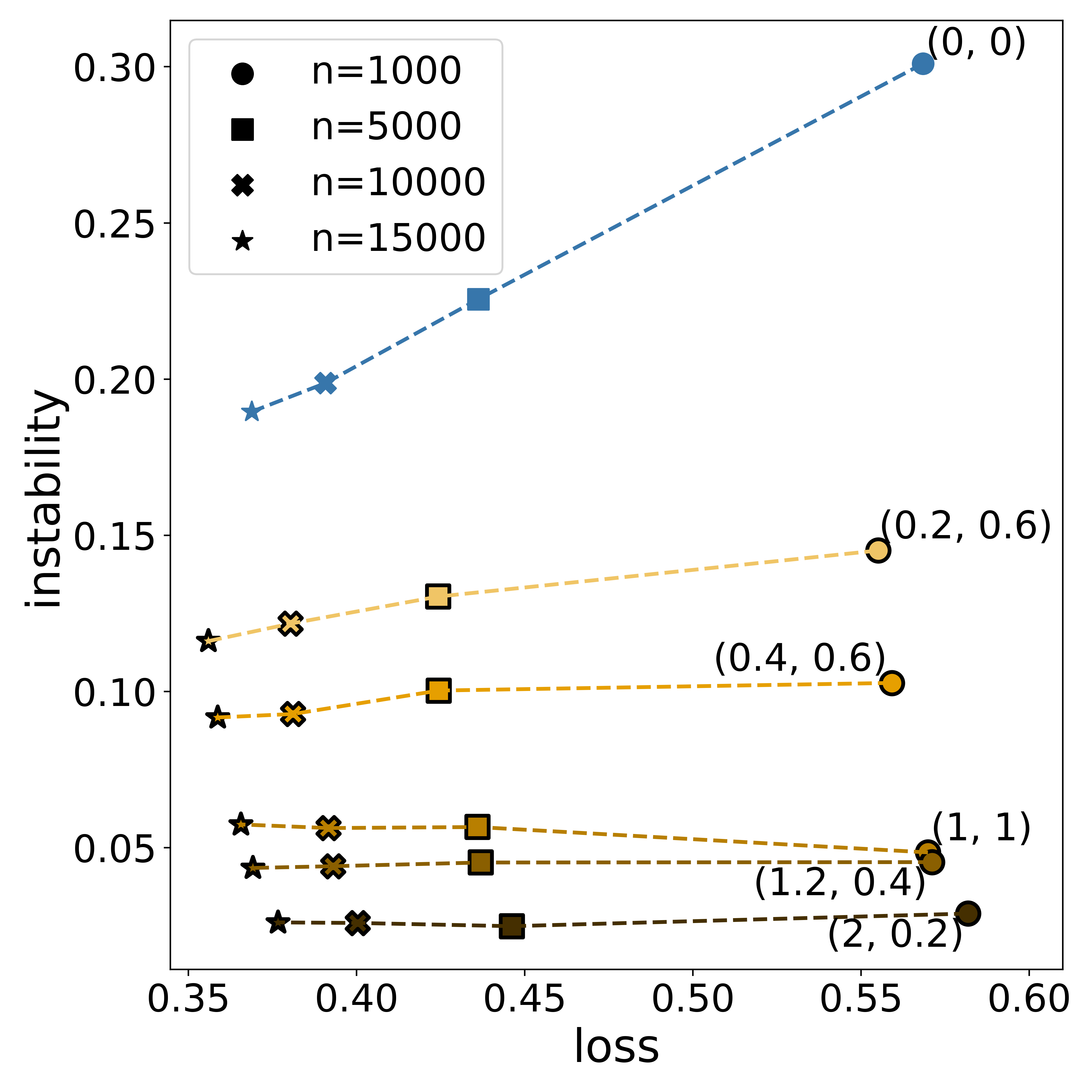
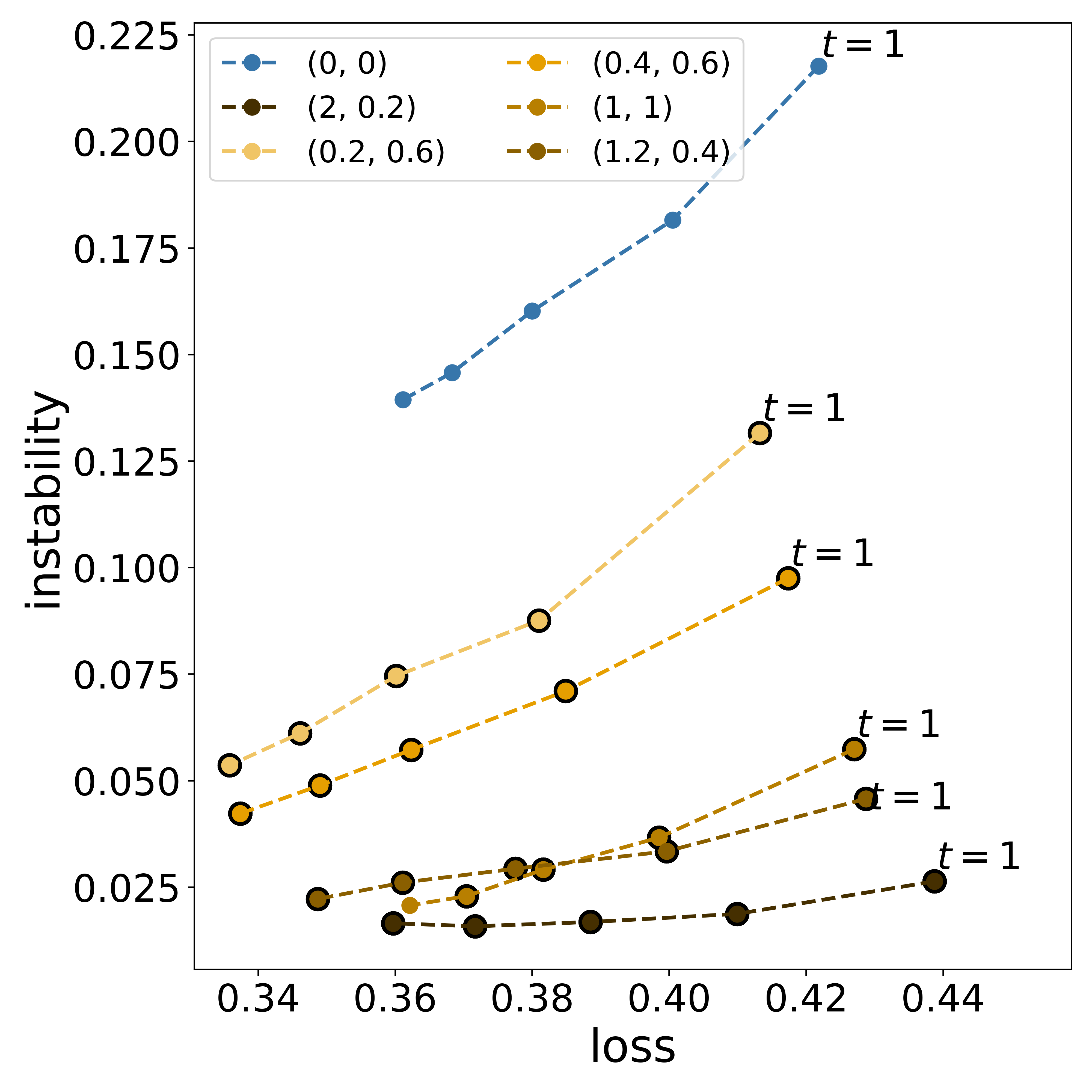
Secondary setups. Two additional experiments are conducted using the California dataset. We select five different hyperparameter configurations from the Pareto-efficient configurations identified in the main setup, each representing a different trade-off. The varied sample sizes setup uses 5000 data points as test data to compute loss and stability. The dataset is obtained by samples samples without replacement from the remaining data. Half of represents . An initial model is trained on and updated using . We run the experiment for different values of and repeat it 50 times and average loss and stability estimates on test data. The iterative updates setup divides the dataset into seven folds, where one fold serves as and one serves as test data. The remaining five folds represent additional information, , obtained at different update iterations. An initial model is trained on . For each update iteration a fold is added to to obtain and the model is updated and evaluated on the test data. The experiment is repeated 50 times and averages loss and stability estimates on test data.
5.2 Experimental Results
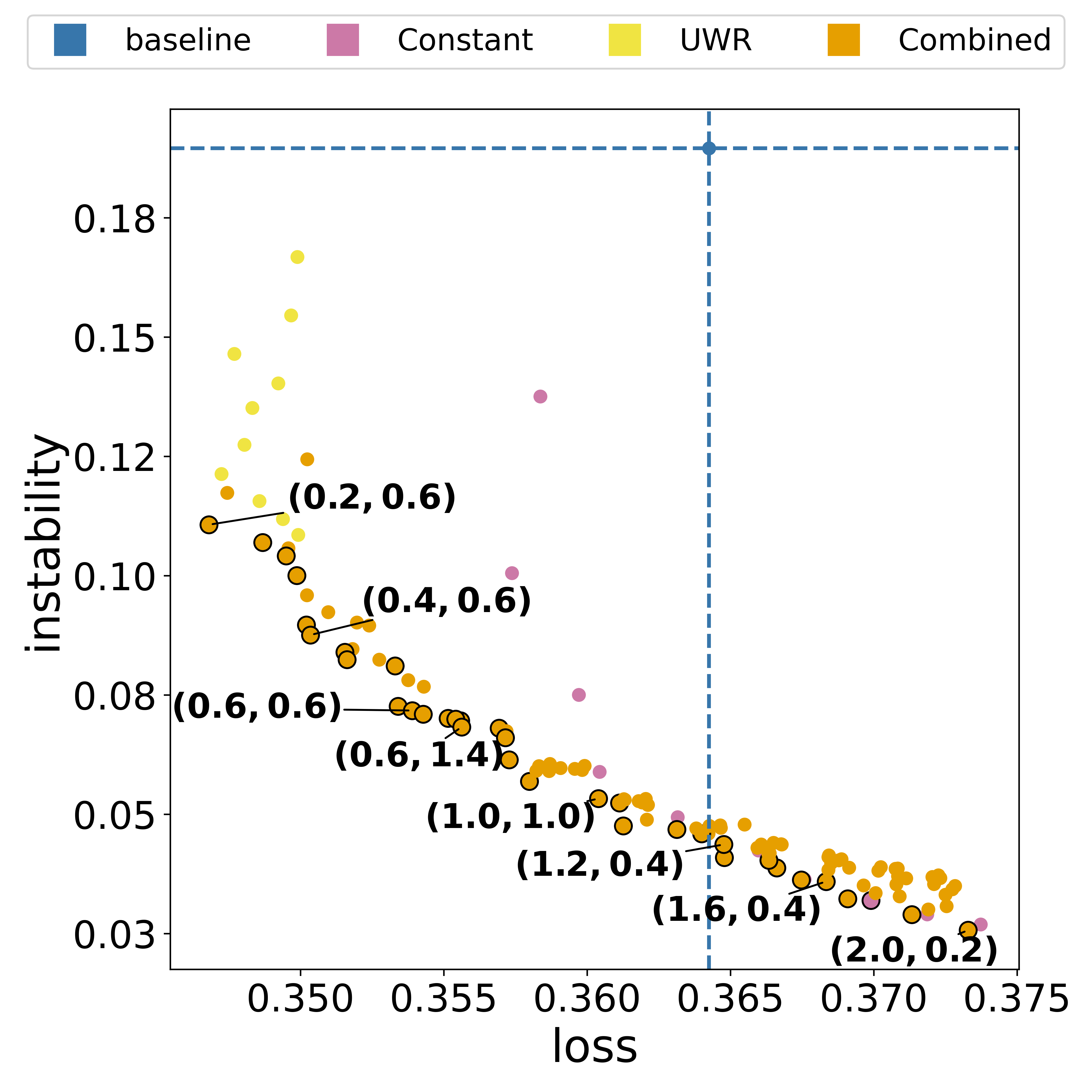
Figure 2 shows the results of the main experiment for the California dataset. The baseline is the least stable model and is not on the Pareto frontier. As we introduce regularization, more predictive and/or stable solutions can be achieved by tuning and . The constant approach shows a consistent reduction in instability as increases and up to a certain value, it also reduces loss. The UWR approach results in more stable models than the baseline with lower loss compared to both the baseline and constant approach. The combination of the constant and the UWR approach leads to better solutions than the pure constant and UWR solutions, showcased by the Pareto frontier.
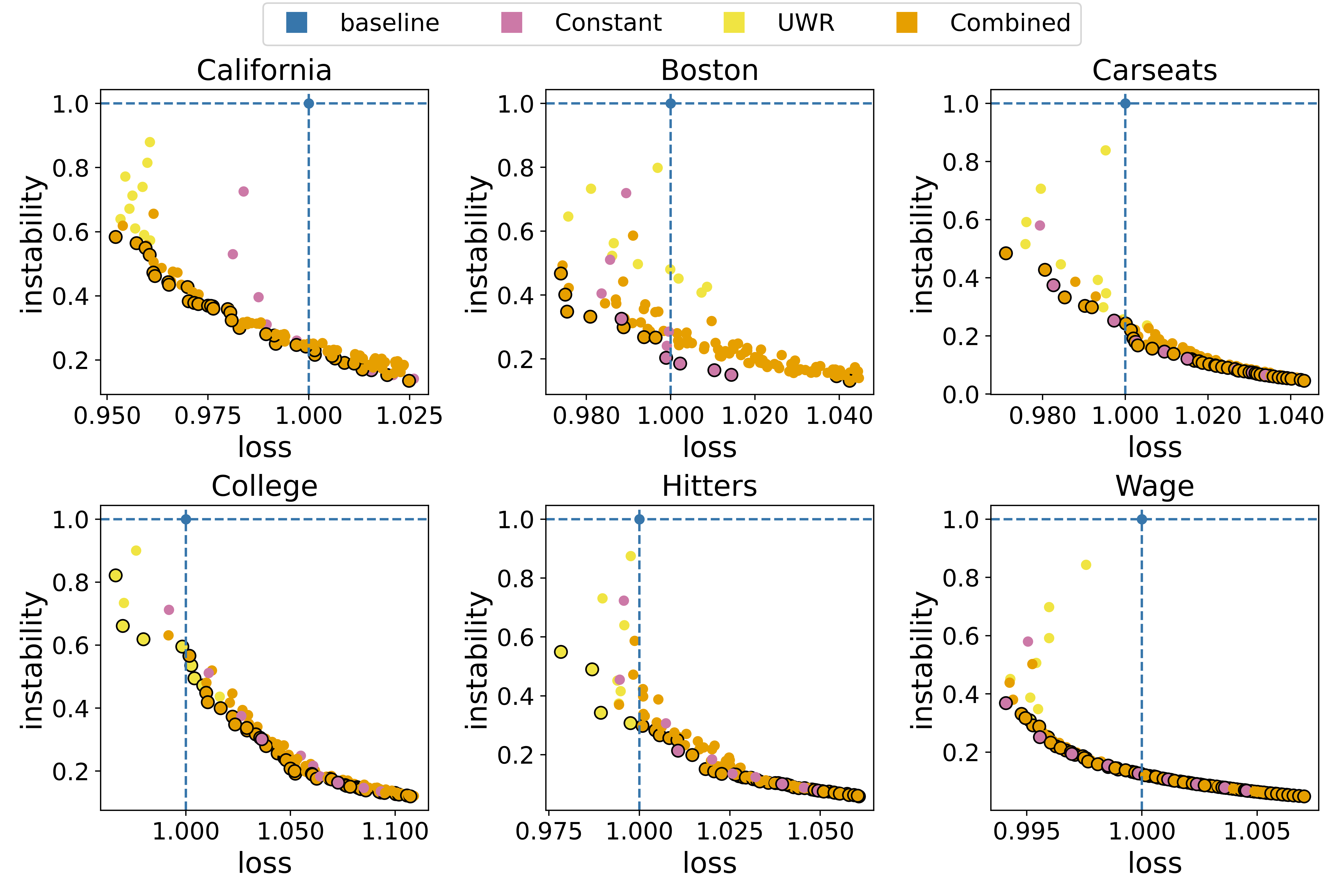
Figure 3 shows and compares the results of the main experiment for all six datasets. Notably, the baseline does not appear on the Pareto frontier for any of the datasets, with all (, ) configurations being more stable. Furthermore, many configurations also achieve lower loss than the baseline. Comparing the constant and UWR approaches, the constant approach tends to lead to more stable solutions, whereas the UWR approach tends to achieve lower loss, although there is an exception for Wage datasets. The combined approach frequently finds Pareto-efficient solutions that are unattainable by either the constant or UWR approaches in isolation.
The result of the varied sample size experiment (Figure 4(a)) shows that loss and stability decrease with larger sample sizes for baseline. For the five selected (, ) configurations, loss decreases while instability remains around the same level. Among the six models, all five configurations are always on the Pareto frontier for all sample sizes. The configurations are consistently more stable than the baseline at corresponding sample sizes. The configurations (0.2, 0.6) and (0.4, 0.6) also consistently achieve lower losses than the baseline.
Figure 4(b) presents the result of five selected (, ) configurations over five update iterations. Compared to the baseline, each configuration achieves improved stability at all update iterations. At the first update iteration, the configurations (0.2, 0.6) and (0.4, 0.6) achieve a lower loss than the baseline and at the second update iteration, also configurations (1, 1) and (1.2, 0.4) achieve a lower loss. The next iteration, (1, 1) becomes more stable than (1.2, 0.4) but with a higher loss than the baseline. By the final update iteration, all configurations except (1, 1) result in a more predictive solution than the baseline. At the first iteration, all configurations are Pareto-efficient solutions, where the configurations (0.2, 0.6), (0.4, 0.6), (1.2, 0.4) and (2, 0.2) are Pareto-efficient models across all update iterations. Note that in practice one would not stick to one configuration across all updates, but rather do a hyperparameter search for each update iteration.
6 Discussion
The objective of this paper was to provide stable updates for regression trees that better balance the predictability-stability trade-off. We propose a regularization method with two tunable hyperparameters. Through a series of experiments conducted across various datasets and conditions, we demonstrated the limitations of the baseline approach. Compared to our method, the baseline consistently fails to be on the Pareto frontier, suggesting the necessity of regularization to achieve a better trade-off. As we explore the regularization landscape by adjusting and , we observe a diverse set of Pareto efficient solutions, each representing a unique balance between predictability and stability.
The main experiment on the California dataset revealed that the constant approach tends to be more stability-focused as stability is equally important for each data point. Incrementally increasing the constant regularization factor consistently improves model stability and up to a certain value of also improves predictability. Conversely, the UWR approach tends to be more predictability-focused as stability for predictions in uncertain regions of receives less weight. The fact that UWR often improves predictability demonstrates the benefit of utilizing prediction uncertainty for regularization. Combining the two approaches leads us to a spectrum of Pareto-efficient solutions, where we can strategically choose (, ) configurations based on the desired predictability-stability trade-off. These findings showcase that both regularization approaches are relevant. Furthermore, these results also extend to the other datasets, demonstrating the generalizability of our approach. Across all datasets, the baseline is never one of the Pareto-efficient models. All (, ) configurations led to more stable models with many configurations also achieving lower loss.
Our secondary experiments showed that our regularization method gives consistent results regardless of sample size and that the benefits of our method extend over multiple updates. When updating multiple times, our method continues to outperform the baseline in terms of predictability and/or stability. The models with lower and values are the most predictive with steady improvements in stability, while the models with large and small are the most stable and remain at the same stability level across updates, with steady improvements in predictability. Having large and values seems to quickly become too stability-focused, which comes at the cost of predictability.
A good choice of hyperparameters depends on the user’s preference. Conservative users might prefer stability and therefore opt for larger and/or values, while users primarily concerned with performance would rather opt for lower values. In practice, users should specify a stability threshold before model selection.
A notable constraint of our approach is the requirement for batch training, needing all available data to update the model. This is necessary as the CART algorithm, on which our updating strategy relies, is a batch algorithm. Future work could explore ways to remove the reliance on previous data to make the method fit in an incremental learning setting.
The focus of our study was on regression tasks using squared error loss. It would be interesting to apply stable updates of tree models to other tasks, such as classification or survival analysis and use other types of loss and instability functions, such as log loss and Poisson loss. This would also expand the potential for industry applications.
While we show that our method improves the empirical stability of regression trees in terms of semantic stability, we do not consider structural stability in this paper. Structural stability is more directly related to explainability and therefore of substantial interest. Investigating how our method influences the structural stability of trees is a valuable direction for future research.
Our results show that iterative updates improve predictability. This leads us to the following untested hypothesis: Learning a regression tree by starting with a subset of the data and iteratively incorporating more data using our update method improves upon the CART algorithm. This raises the questions of how large the subset should be and how many updates to perform.
Lastly, our focus has been solely on individual regression trees. An interesting extension would be to investigate how our method works in an ensemble setting like random forests.
In conclusion, stable regression trees provide a good way of balancing the predictability-stability trade-off, highlighted by its ability to outperform the baseline approach across various datasets, data sizes and multiple update iterations.
Acknowledgments
NB was supported in part by the Research Council of Norway grant “Parameterized Complexity for Practical Computing (PCPC)” (NFR, no. 274526).
References
- Blørstad (2023) Morten Blørstad. Improving Stability of Tree-Based Models. Master’s thesis, University of Bergen, Bergen, 2023.
- Bousquet & Elisseeff (2002) Olivier Bousquet and André Elisseeff. Stability and Generalization. J. Mach. Learn. Res., 2:499–526, 3 2002. ISSN 1532-4435. doi: 10.1162/153244302760200704. URL https://doi.org/10.1162/153244302760200704.
- Breiman et al. (1984) L Breiman, Jerome H Friedman, Richard A Olshen, and C J Stone. Classification and Regression Trees. New York, 1st edition edition, 1984. doi: https://doi.org/10.1201/9781315139470.
- Breiman (1996) Leo Breiman. Bagging predictors. Machine Learning, 24(2):123–140, 1996. ISSN 1573-0565. doi: 10.1007/BF00058655. URL https://doi.org/10.1007/BF00058655.
- Briand et al. (2009) Bénédicte Briand, Gilles R Ducharme, Vanessa Parache, and Catherine Mercat-Rommens. A similarity measure to assess the stability of classification trees. Computational Statistics & Data Analysis, 53(4):1208–1217, 2009. ISSN 0167-9473. doi: https://doi.org/10.1016/j.csda.2008.10.033. URL https://www.sciencedirect.com/science/article/pii/S0167947308004970.
- Burnham & Anderson (2004) Kenneth P. Burnham and David R. Anderson. Model Selection and Multimodel Inference. Springer New York, New York, NY, 2004. ISBN 978-0-387-95364-9. doi: 10.1007/b97636.
- Chen & Guestrin (2016) Tianqi Chen and Carlos Guestrin. XGBoost: A Scalable Tree Boosting System. arXiv, 3 2016. doi: 10.1145/2939672.2939785. URL https://arxiv.org/abs/1603.02754.
- Cotter et al. (2018) Andrew Cotter, Heinrich Jiang, Serena Wang, Taman Narayan, Maya Gupta, Seungil You, and Karthik Sridharan. Optimization with Non-Differentiable Constraints with Applications to Fairness, Recall, Churn, and Other Goals, 2018.
- Cox et al. (1985) John C Cox, Jonathan E Ingersoll, and Stephen A Ross. A Theory of the Term Structure of Interest Rates. Econometrica, 53(2):385–407, 1985. ISSN 00129682, 14680262. doi: 10.2307/1911242. URL http://www.jstor.org/stable/1911242.
- Dannegger (2000) Felix Dannegger. Tree stability diagnostics and some remedies for instability. Statistics in medicine, 19:475–491, 1 2000. doi: 10.1002/(SICI)1097-0258(20000229)19:43.0.CO;2-V.
- Devroye & Wagner (1979) L Devroye and T Wagner. Distribution-free performance bounds for potential function rules. IEEE Transactions on Information Theory, 25(5):601–604, 1979. doi: 10.1109/TIT.1979.1056087.
- Goh et al. (2016) Gabriel Goh, Andrew Cotter, Maya Gupta, and Michael P Friedlander. Satisfying Real-world Goals with Dataset Constraints. In D D Lee, M Sugiyama, U V Luxburg, I. Guyon, and R Garnett (eds.), Advances in Neural Information Processing Systems 29, pp. 2415–2423. 2016.
- Hastie et al. (2001) Trevor Hastie, Robert Tibshirani, and Jerome Friedman. The Elements of Statistical Learning. Springer New York, New York, NY, 2001. ISBN 978-0-387-84857-0. doi: 10.1007/978-0-387-84858-7.
- Huber (1967) Peter J Huber. The behavior of maximum likelihood estimates under nonstandard conditions. 1967. URL https://api.semanticscholar.org/CorpusID:123642812.
- James et al. (2022) Gareth James, Daniela Witten, Trevor Hastie, Rob Tibshirani, and Balasubramanian Narasimhan. ISLR2. Technical report, packaged 2022-11-20, 2022.
- Kaminski & Malgieri (2021) Margot E Kaminski and Gianclaudio Malgieri. Algorithmic impact assessments under the GDPR: producing multi-layered explanations. International Data Privacy Law, 11(2):125–144, 4 2021. ISSN 2044-3994. doi: 10.1093/idpl/ipaa020. URL https://doi.org/10.1093/idpl/ipaa020.
- Kearns & Ron (1999) Michael Kearns and Dana Ron. Algorithmic Stability and Sanity-Check Bounds for Leave-One-Out Cross-Validation. Neural Computation, 11(6):1427–1453, 7 1999. ISSN 0899-7667. doi: 10.1162/089976699300016304. URL https://doi.org/10.1162/089976699300016304.
- Kelley Pace & Barry (1997) R Kelley Pace and Ronald Barry. Sparse spatial autoregressions. Statistics & Probability Letters, 33(3):291–297, 1997. ISSN 0167-7152. doi: https://doi.org/10.1016/S0167-7152(96)00140-X. URL https://www.sciencedirect.com/science/article/pii/S016771529600140X.
- Last et al. (2002) Mark Last, Oded Maimon, and Einat Minkov. Improving Stability of Decision Trees. International Journal of Pattern Recognition and Artificial Intelligence, 16(02):145–159, 2002. doi: 10.1142/S0218001402001599. URL https://doi.org/10.1142/S0218001402001599.
- Lim & Yu (2013) Chinghway Lim and B Yu. Estimation Stability with Cross Validation (ESCV). Journal of Computational and Graphical Statistics, 25, 1 2013. doi: 10.1080/10618600.2015.1020159.
- Lin et al. (2002) Lawrence Lin, A. S Hedayat, Bikas Sinha, and Min Yang. Statistical Methods in Assessing Agreement. Journal of the American Statistical Association, 97(457):257–270, 2002. doi: 10.1198/016214502753479392. URL https://doi.org/10.1198/016214502753479392.
- Liu et al. (2022) Huiting Liu, Avinesh S., Siddharth Patwardhan, Peter Grasch, and Sachin Agarwal. Model Stability with Continuous Data Updates, 2 2022.
- Lunde et al. (2020) Berent Ånund Strømnes Lunde, Tore Selland Kleppe, and Hans Julius Skaug. An information criterion for automatic gradient tree boosting. arXiv, 8 2020. doi: 10.48550/arxiv.2008.05926. URL https://arxiv.org/abs/2008.05926.
- Milani Fard et al. (2016) Mahdi Milani Fard, Quentin Cormier, Kevin Canini, and Maya Gupta. Launch and Iterate: Reducing Prediction Churn. In D Lee, M Sugiyama, U Luxburg, I Guyon, and R Garnett (eds.), Advances in Neural Information Processing Systems, volume 29. Curran Associates, Inc., 2016. URL https://proceedings.neurips.cc/paper_files/paper/2016/file/dc5c768b5dc76a084531934b34601977-Paper.pdf.
- Philipp et al. (2017) Michel Philipp, Thomas Rusch, Kurt Hornik, and Carolin Strobl. Measuring the Stability of Results From Supervised Statistical Learning. Journal of Computational and Graphical Statistics, 131, 1 2017. doi: 10.1080/10618600.2018.1473779.
- Takeuchi (1976) K Takeuchi. Distribution of information statistics and validity criteria of models. Mathematical Science, 153:12–18, 5 1976.
- Turney (1995) Peter Turney. Technical Note: Bias and the Quantification of Stability. Machine Learning, 20:23–33, 7 1995. doi: 10.1007/BF00993473.