Adaptive Ridge Approach to Heteroscedastic Regression

Abstract.

We propose an adaptive ridge (AR) based estimation scheme for a heteroscedastic linear model equipped with log-linear errors. We simultaneously estimate the mean and variance parameters and show new asymptotic distributional and tightness properties in a sparse setting. We also show that estimates for zero parameters shrink with more iterations under suitable assumptions for tuning parameters. We observe possible generalizations of this paper’s results through simulations and will apply the estimation method in forecasting electricity consumption.

1. Introduction

Consider the following location-scale regression model

$$Y_{i}=X_{i}\alpha+e^{\frac{1}{2}Z_{i}\beta}\epsilon_{i},\quad\text{for }i=1,...,n$$ (1.1)

for one-dimensional responses $Y_{i}$, covariates $X_{i}=(X_{i1},...,X_{ip})\in\mathbb{R}^{p}$ and $Z_{i}=(Z_{i1},...,Z_{iq})\in\mathbb{R}^{q}$ with log-linear errors. The model can also be written as

$$Y=X\alpha+D_{n}(Z;\beta)\epsilon,$$ (1.2)

where $X\in\mathbb{R}^{n\times p}$ and $Z\in\mathbb{R}^{n\times q}$ are the design matrices, $Y\in\mathbb{R}^{n}$ is the response, $\epsilon\in\mathbb{R}^{n}$ is the error and $D_{n}(Z;\beta)=D_{n}(\beta):={\rm diag}(e^{\frac{1}{2}Z_{1}\beta},...,e^{\frac{1}{2}Z_{n}\beta})$. The covariates $X$ and $Z$ may have common components.

The seminal work [8] introduced ridge estimators to tackle multicollinearity, an issue that made the ordinary least squares estimator unreliable. Taking advantage of the availability of the explicit form of ridge estimators, we propose an adaptive ridge estimator to estimate the unknown parameter $\theta_{0}:=(\alpha_{0},\beta_{0})=(\alpha_{01},...,\alpha_{0p},\beta_{01},...,\beta_{0q})\in\Theta_{\alpha}\times\Theta_{\beta}\subseteq\mathbb{R}^{p}\times\mathbb{R}^{q}$ for bounded domains $\Theta_{\alpha}$ and $\Theta_{\beta}$. We introduce a computationally efficient estimator that does not require numerical optimization. We also carefully consider variable selection without fully committing to a sparse regularization, which is known to be fragile if true parameters are small but non-zero.

The model under (1.1) was first studied in 1976 by [7] using an approach utilizing the least squares regression and then the likelihood analysis for normal errors. We will not restrict to normal errors in this paper, as we discuss conditions required for asymptotics to hold. In particular, we show asymptotic results for the scale parameter $\beta$ that were absent in [7] and subsequent works studying this model.

Results for penalized estimators are widely studied, as in [6]. A similar iterative approach is the Broken Adaptive Ridge (BAR) estimator for the parameter $\alpha$, under a setting without including exponentially-scaled errors [2]. Our adaptive ridge (AR) estimator is an iterative procedure that estimates $\alpha$ and $\beta$ in alternation. We empirically show that our estimators can strike a balance between computational ease and stability for small non-zero parameters, see for instance [6] and [10]. Altogether, we take a practical standpoint and simultaneously tackle multiple statistical settings such as multiplicative heteroscedasticity, and sparsity.

We organize the paper as follows. We introduce notation and the setup of the AR procedure in Section 2. In Section 3, we first state the assumptions, and then prove asymptotic distributional results for the initial and iterated estimators of $\alpha$ and $\beta$ in 3.5 and 3.6, respectively. Then, we justify the reason to perform more iterations in 3.9. Simulation results are given in Section 4 and we compare the performance of AR with other well-known regularized estimators using electricity consumption data in Section 5. We discuss unresolved issues in Section 6 with concluding remarks and defer our proofs to the Appendix.

2. Constructing the Adaptive Ridge Estimators

We begin by describing the AR procedure, defining the estimators, and introducing the required notation. We will denote the transpose of matrices and vectors by $A^{T}$ and $v^{T}$, respectively. Furthermore, we will take exponentials, logarithms, and powers of vectors component-wise. Throughout this paper, unless otherwise specified, $\|\cdot\|$ stands for the Euclidean norm for vectors and the spectral norm of matrices, so that for any square matrix $A$, $\|A\|$ is the square root of the largest eigenvalue of $A^{T}A$. We denote positive definite matrices by $A\succ 0$ and positive semi-definite matrices by $A\succeq 0$. For a diagonal matrix, this is equivalent to having positive and non-negative entries. We will use $\xrightarrow{\mathcal{L}}$ for convergence in law and $\xrightarrow{p}$ for convergence in probability. We write $\lambda_{\min}(A)$ and $\lambda_{\max}(A)$ for the minimum and maximum eigenvalues of a matrix $A$. Finally, we will use the notation $X_{n}\lesssim Y_{n}$ to mean for some universal constant $C$, $X_{n}\leq CY_{n}$ for every large enough $n$.

Define the diagonal tuning parameter matrix $\Lambda_{n}:={\rm diag}(\lambda_{n1},...,\lambda_{np})\succeq 0$. The initial ridge estimator corresponding to $\Lambda_{n}$ is:

$$\tilde{\alpha}^{(0)}_{n}:=\operatorname*{arg\,min}_{\alpha\in\mathbb{R}^{p}}\left\{\|Y-X\alpha\|^{2}+\alpha^{T}\Lambda_{n}\alpha\right\}=(X^{T}X+\Lambda_{n})^{-1}X^{T}Y.$$ (2.1)

We aim to construct a ridge estimator for $\beta$ by plugging in our estimator of $\alpha$. If we write

$$L_{n}(\alpha)=\left({\rm log}(Y_{1}-X_{1}\alpha)^{2},\dots,{\rm log}(Y_{n}-X_{n}\alpha)^{2}\right)^{T},$$

then

$$L_{n}(\alpha_{0})-Z\beta_{0}={\rm log}(\epsilon^{2}).$$ (2.2)

Assuming $\mathbb{P}[\epsilon_{1}=0]=0$ (see 3.3), (2.2) is well defined almost surely. Then, by subtracting the unknown expectation $\mathbb{E}\left[{\rm log}(\epsilon^{2})\right]$ on both sides, we get

$$L_{n}(\alpha_{0})-Z\beta_{0}-\mathbb{E}\left[{\rm log}(\epsilon^{2})\right]={\rm log}(\epsilon^{2})-\mathbb{E}\left[{\rm log}(\epsilon^{2})\right],$$

which allows us to consider a ridge-type estimator for the zero-mean errors ${\rm log}(\epsilon^{2})-\mathbb{E}\left[{\rm log}(\epsilon^{2})\right]$. Denote

$Z^{\ast}:=(Z,\mathbf{1}_{n})$ and $\beta^{\ast}_{0}:=(\beta_{0}^{T},c_{0})=\left(\beta_{0}^{T},\mathbb{E}\left[{\rm log}(\epsilon_{1}^{2})\right]\right)$,

where $\mathbf{1}_{n}\in\mathbb{R}^{n}$ denotes a column of 1’s. We define the initial ridge estimator of $\beta^{\ast}_{0}\in\mathbb{R}^{q+1}$ to be

$$\begin{split}\tilde{\beta}^{\ast(0)}_{n}=\left(\tilde{\beta}^{(0)}_{n},\tilde{c}^{(0)}_{n}\right)&\coloneqq\operatorname*{arg\,min}_{\beta^{\ast}\in\mathbb{R}^{q+1}}\left\{\|L_{n}(\tilde{\alpha}_{n}^{(0)})-Z^{\ast}\beta^{\ast}\|^{2}+\beta^{\ast T}\Gamma^{\ast}_{n}\beta^{\ast}\right\}\\ &=\left(Z^{\ast T}Z^{\ast}+\Gamma^{\ast}_{n}\right)^{-1}Z^{\ast T}L_{n}(\tilde{\alpha}_{n}^{(0)}),\end{split}$$ (2.3)

where $\Gamma^{\ast}_{n}\coloneqq{\rm diag}(\gamma_{n1},...,\gamma_{nq},\gamma_{n,q+1})\succeq 0$ is the diagonal tuning parameter matrix associated with $\beta^{\ast}$. We will show the asymptotic normality of $\tilde{\alpha}_{n}^{(0)}$ and depending on the strictness of conditions placed on $\epsilon$, tightness or asymptotic normality of $\tilde{\beta}^{\ast(0)}_{n}$ before further deducing the asymptotic results of subsequent estimators.

Remark 2.1.

We assume the matrix $Z$ does not contain a column of $1$’s, which is crucial as we wish to estimate $\mathbb{E}\left[{\rm log}(\epsilon_{1}^{2})\right]$, so an additional intercept term poses an identifiability issue. If a column of 1’s is present, we lose consistency when estimating the intercept term of $\beta$, as there will be bias contributed by the term $\mathbb{E}\left[{\rm log}(\epsilon_{1}^{2})\right]$. We avoid this inconvenience by imposing this assumption, but results for the AR procedure for other components do not depend on this assumption.

Using this estimate for $\beta$, we can define an adaptive weighted ridge estimator for $\alpha$. By letting

$$T(\alpha)\coloneqq{\rm diag}(\alpha_{1}^{-2},...,\alpha_{p}^{-2}),$$

we can define for $k\geq 0$

$$\begin{split}\tilde{\alpha}_{n}^{(k+1)}&\coloneqq\operatorname*{arg\,min}_{\alpha\in\mathbb{R}^{p}}\left\{\|D_{n}^{-1}(\tilde{\beta}_{n}^{(k)})(Y-X\alpha)\|^{2}+\alpha^{T}\Lambda_{n}T(\tilde{\alpha}_{n}^{(k)})\alpha\right\}\\ &=\left(X^{T}D^{-2}_{n}(\tilde{\beta}_{n}^{(k)})X+\Lambda_{n}T(\tilde{\alpha}_{n}^{(k)})\right)^{-1}X^{T}D^{-2}_{n}(\tilde{\beta}_{n}^{(k)})Y.\end{split}$$ (2.4)

We then repeat a process similar to (2.3) upon obtaining an updated estimator for $\alpha$ with adjusted weights in the ridge penalty. Namely, by setting

$$S(\beta^{\ast}):={\rm diag}(\beta_{1}^{-2},...,\beta_{q}^{-2},c^{-2}),$$

for $k\geq 0$ we define an updated estimator of $\beta^{\ast}$ as follows:

$$\begin{split}\tilde{\beta}^{\ast(k+1)}_{n}&=(\tilde{\beta}^{(k+1)}_{n},\tilde{c}^{(k+1)}_{n})\\ &\coloneqq\operatorname*{arg\,min}_{\beta^{\ast}\in\mathbb{R}^{q+1}}\left\{\|L_{n}(\tilde{\alpha}_{n}^{(k+1)})-Z^{\ast}\beta^{\ast}\|^{2}+\beta^{\ast T}\Gamma^{\ast}_{n}S(\tilde{\beta}_{n}^{\ast(k)})\beta^{\ast}\right\}\\ &=\left(Z^{\ast T}Z^{\ast}+\Gamma^{\ast}_{n}S(\tilde{\beta}_{n}^{\ast(k)})\right)^{-1}Z^{\ast T}L_{n}(\tilde{\alpha}_{n}^{(k+1)}).\end{split}$$ (2.5)

Remark 2.2.

Note that since the initial ridge estimators $\tilde{\alpha}_{n}^{(0)}$ and $\tilde{\beta}_{n}^{(0)}$ and their subsequent iterations are non-zero almost surely, $T(\alpha)$ and $S(\beta^{\ast})$ are well defined.

In our proposed method, we will have to divide by very small, non-zero values in the matrix $T(\alpha)$ when the estimates of $\alpha$ are small, in turn causing arithmetic overflow [2]. One solution given in [5] to circumvent this issue is by introducing a small perturbation by defining $T(\alpha)={\rm diag}\left(\frac{1}{(\alpha_{1})^{2}+\delta_{\alpha}},..,\frac{1}{(\alpha_{p})^{2}+\delta_{\alpha}}\right)$ and $S(\beta^{\ast})={\rm diag}\left(\frac{1}{(\beta_{1})^{2}+\delta_{\beta}},..,\frac{1}{(\beta_{q})^{2}+\delta_{\beta}},\frac{1}{c^{2}+\delta_{\beta}}\right)$ for some small constants $\delta_{\alpha},\delta_{\beta}>0$, which improves numerical stability at the cost of introducing some bias and fitting two extra hyperparameters.

We choose to adopt another method proposed [11] and [2]. By denoting

$$\tilde{X}^{(k)}_{n}:=D_{n}^{-1}(\tilde{\beta}^{(k)}_{n})XT^{-\frac{1}{2}}(\tilde{\alpha}^{(k)}_{n})\hskip 14.22636pt\text{and}\hskip 14.22636pt\tilde{Y}^{(k)}_{n}:=D_{n}^{-1}(\tilde{\beta}^{(k)}_{n})Y,$$

we can write

$$\tilde{\alpha}^{(k+1)}_{n} =\left(X^{T}D^{-2}_{n}(\tilde{\beta}_{n}^{(k)})X+\Lambda_{n}T(\tilde{\alpha}_{n}^{(k)})\right)^{-1}X^{T}D^{-2}_{n}(\tilde{\beta}_{n}^{(k)})Y$$

$$=\left(T^{\frac{1}{2}}(\tilde{\alpha}_{n}^{(k)})\left(T^{-\frac{1}{2}}(\tilde{\alpha}_{n}^{(k)})X^{T}D^{-2}_{n}(\tilde{\beta}_{n}^{(k)})XT^{-\frac{1}{2}}(\tilde{\alpha}_{n}^{(k)})+\Lambda_{n}\right)T^{\frac{1}{2}}(\tilde{\alpha}_{n}^{(k)})\right)^{-1}X^{T}D^{-2}_{n}(\tilde{\beta}_{n}^{(k)})Y$$

$$=T^{-\frac{1}{2}}(\tilde{\alpha}^{(k)}_{n})\left(T^{-\frac{1}{2}}(\tilde{\alpha}_{n}^{(k)})X^{T}D^{-2}_{n}(\tilde{\beta}_{n}^{(k)})XT^{-\frac{1}{2}}(\tilde{\alpha}_{n}^{(k)})+\Lambda_{n}\right)^{-1}T^{-\frac{1}{2}}(\tilde{\alpha}^{(k)}_{n})X^{T}D^{-2}_{n}(\tilde{\beta}_{n}^{(k)})Y$$

$$=T^{-\frac{1}{2}}(\tilde{\alpha}^{(k)}_{n})\left(\tilde{X}^{(k)T}_{n}\tilde{X}^{(k)}_{n}+\Lambda_{n}\right)^{-1}\tilde{X}^{(k)T}_{n}\tilde{Y}^{(k)}_{n}.$$

Similarly, by writing

$$\tilde{Z}^{\ast(k)}_{n}:=Z^{\ast}S^{-\frac{1}{2}}(\tilde{\beta}^{\ast(k)}_{n}),$$

we get

$$\tilde{\beta}^{\ast(k+1)}_{n}=S^{-\frac{1}{2}}(\tilde{\beta}^{\ast(k)}_{n})\left(\tilde{Z}^{\ast(k)T}_{n}\tilde{Z}^{\ast(k)}_{n}+\Gamma^{\ast}_{n}\right)^{-1}\tilde{Z}^{\ast(k)T}_{n}L_{n}(\tilde{\alpha}^{(k)}_{n}),$$

allowing us to deal with most stability issues without fitting two extra tuning parameters.

It is important to note that the expressions (2.1), (2.3), (2.4), and (2.5) have closed forms and thus require no numerical optimization, which is an advantage over many other existing methods in terms of computational efficiency. The AR scheme is therefore very scalable into higher dimensions.

3. Main results

3.1. Assumptions

Assumption 3.1.

There exist positive definite matrices $\Sigma^{X}$, $\Sigma^{X}_{+}$, $\Sigma^{X}_{-}$, $\Sigma^{Z}$ and $\Sigma^{Z^{\ast}}$ such that

$$\begin{gathered}\frac{X^{T}X}{n}\to\Sigma^{X},\frac{X^{T}D_{n}^{2}(\beta_{0})X}{n}\to\Sigma^{X}_{+}\text{ and }\frac{X^{T}D_{n}^{-2}(\beta_{0})X}{n}\to\Sigma^{X}_{-}\\ \frac{Z^{T}Z}{n}\to\Sigma^{Z}\text{ and }\frac{Z^{\ast T}Z^{\ast}}{n}\to\Sigma^{Z^{\ast}}\end{gathered}$$ (3.1)

as $n\to\infty$. Furthermore, there exist constants $K_{X}>1$, $K_{Z}>1$, and $N\in\mathbb{N}$ for which

$$\frac{1}{K_{X}}\leq\inf_{n\geq N}\inf_{\beta}\lambda_{min}\left(\frac{X^{T}D^{-2}_{n}(\beta)X}{n}\right)\leq\sup_{n\geq N}\sup_{\beta}\lambda_{max}\left(\frac{X^{T}D^{-2}_{n}(\beta)X}{n}\right)\leq K_{X},$$

$$\frac{1}{K_{Z}}\leq\inf_{n\geq N}\lambda_{min}\left(\frac{Z^{\ast T}Z^{\ast}}{n}\right)\leq\sup_{n\geq N}\lambda_{max}\left(\frac{Z^{\ast T}Z^{\ast}}{n}\right)\leq K_{Z}.$$ (3.2)

Assumption 3.2.

$$\sup_{n}\|X_{n}\|<\infty\text{ and }\sup_{n}\|Z^{\ast}_{n}\|<\infty.$$

Assumption 3.3.

The random errors $\epsilon_{1},\epsilon_{2},...$ are i.i.d. with $\mathbb{E}\left[\epsilon_{1}\right]=0$, ${\rm var}[\epsilon_{1}]=1$. Furthermore, $\mathbb{E}\left[|\epsilon_{1}|^{-s}\right]<\infty$ for all $s\in(-\infty,1)$.

Assumption 3.4.

For each $k\geq 0$, there exists some $a\in(0,1)$ and $N$ such that

$$\sup_{n>N}\sup_{i}\mathbb{E}\left[\left|e^{\frac{1}{2}Z_{i}\beta_{0}}\epsilon_{i}-X_{i}(\tilde{\alpha}_{n}^{(k)}-\alpha_{0})\right|^{-a}\right]<\infty.$$

3.1, 3.2 and the mean and variance conditions of 3.3 are standard to make. The rest are regularity conditions tailored to proving asymptotic results of $\beta$. The negative moments conditions of 3.3 and 3.4 can be verified by considering densities when they exist [9], which we will further explain after stating 3.5. Note that the logarithmic moments $\mathbb{E}[{\rm log}(\epsilon)]$ and $\mathbb{E}[{\rm log}(\epsilon^{2})]$ also exist under 3.3.

3.2. Asymptotic results of $\tilde{\alpha}_{n}^{(0)}$ and $\tilde{\beta}_{n}^{\ast(0)}$

We provide an asymptotic result for our initial estimators. As we construct an iterative scheme, the following convergences will play a vital role in asymptotic results for subsequent estimators. The following result for $\alpha$ is well known and is present in literature such as [6]. The asymptotic results for $\beta$ are first proved here to the authors’ understanding.

Theorem 3.5.

Under Assumptions 3.1 to 3.3, if $\dfrac{\Lambda_{n}}{\sqrt{n}}\to\Lambda_{0}$ as $n\to\infty$ for some constant matrix $\Lambda_{0}$, then $\tilde{\alpha}_{n}^{(0)}$ is asymptotically normal:

$$\sqrt{n}\left(\tilde{\alpha}^{(0)}_{n}-\alpha_{0}\right)\xrightarrow{\mathcal{L}}N\left(-(\Sigma^{X})^{-1}\Lambda_{0}\alpha_{0},\,(\Sigma^{X})^{-1}\Sigma^{X}_{+}(\Sigma^{X})^{-1}\right).$$ (3.3)

If 3.4 also holds and $\frac{\Gamma_{n}^{\ast}}{\sqrt{n}}\to 0$, then $\tilde{\beta}^{\ast(0)}_{n}$ is a consistent estimator of $\beta^{\ast}_{0}$. Moreover, for all $c\in[0,\frac{1}{2})$,

$$n^{c}\left(\tilde{\beta}^{\ast(0)}_{n}-\beta^{\ast}_{0}\right)=\mathcal{O}_{p}(1).$$ (3.4)

Furthermore, if $\mathbb{E}\left[|\epsilon_{1}|^{-(1+\tau)}\right]<\infty$ for some $\tau>0$, then $\tilde{\beta}^{\ast(0)}_{n}$ is asymptotically normal:

$$\sqrt{n}\left(\tilde{\beta}^{\ast(0)}_{n}-\beta^{\ast}_{0}\right)\xrightarrow{\mathcal{L}}N\left(0,\left(\Sigma^{Z^{\ast}}\right)^{-1}{\rm var}\left[{\rm log}(\epsilon_{1}^{2})\right]\right).$$ (3.5)

Although we have stated a general result for $\frac{\Lambda_{n}}{\sqrt{n}}\to\Lambda_{0}$, we will focus on $\frac{\Lambda_{n}}{\sqrt{n}}\to 0$ for the rest of this paper. Moreover [9] provides a link between negative moments and the density function (when it exists), which will help understand the negative moments condition needed for (3.5), as well as 3.3 and 3.4. To summarize, [9] showed that if $|\epsilon_{1}|$ possesses a density function $f$, then

1. If $f$ is bounded near $0$ then $\mathbb{E}\left[|\epsilon_{1}|^{-s}\right]<\infty$ for all $0<s<1$.

2. $f(0)>0$ is sufficient for $\mathbb{E}\left[|\epsilon_{1}|^{-1}\right]=\infty$.

3. If for some $\delta>0$, $\lim_{x\to 0^{+}}\frac{f(x)}{x^{\delta}}=K$ for some $K\in(0,\infty)$, then $\mathbb{E}\left[|\epsilon_{1}|^{-(1+\tau)}\right]$ exists for all $0<\tau<\delta$.

Referring to these conditions, it is straightforward to see that most errors, including normal errors, satisfy the condition needed for $\mathbb{E}\left[|\epsilon_{1}|^{-s}\right]<\infty$ for all $0<s<1$ in 3.3, but fail to possess an inverse first moment, which is why (3.4) and (3.5) are presented separately. Still, there are families of distribution that satisfy the condition in (3), for instance, one can show that the log-normal distribution (reflected about $x=0$ and standardized) is a class of errors that satisfy the stricter conditions.

3.4 remains challenging to check, but by (1) it is sufficient to prove for each $k$, there is some sufficiently large $N$ so that

$$\limsup_{u\to 0}\sup_{n>N}\sup_{i=1,...,n}f^{(k)}_{n,i}(u)<\infty,$$

where $f^{(k)}_{n,i}(u)$ denotes the density of $\left|e^{\frac{1}{2}Z_{i}\beta_{0}}\epsilon_{i}-X_{i}(\tilde{\alpha}_{n}^{(k)}-\alpha_{0})\right|$ when it exists. We have shown in (3.3) that $(\tilde{\alpha}_{n}^{(0)}-\alpha_{0})=\mathcal{O}_{p}\left(\frac{1}{\sqrt{n}}\right)$, therefore so is $X_{i}(\tilde{\alpha}_{n}^{(0)}-\alpha_{0})$. We will iteratively show in later parts the same for $k\geq 1$ that $(\tilde{\alpha}_{n}^{(k)}-\alpha_{0})=\mathcal{O}_{p}\left(\frac{1}{\sqrt{n}}\right)$.

3.3. Notation Under Sparsity

We are mainly interested in the asymptotic behavior of estimators under a sparse model, so for clarity we introduce additional notation for subsequent parts. Suppose exactly $0\leq p_{0}\leq p$ and $0\leq q_{0}\leq q+1$ components from $\alpha_{0}$ and $\beta^{\ast}_{0}$ are non-zero. We will denote using the ($\star$) and ($\circ$) subscripts for the non-zero and zero components respectively. Upon permuting the components, $\alpha_{0}=(\alpha_{0\star},\alpha_{0\circ})=(\alpha_{0\star},0,..,0)$ and $\beta^{\ast}_{0}=(\beta^{\ast}_{0\star},\beta^{\ast}_{0\circ})=(\beta^{\ast}_{0\star},0,..,0)$. We will therefore write $\alpha^{(k)}_{n}=(\alpha^{(k)}_{n\star},\alpha^{(k)}_{n\circ})$ and $\beta^{\ast(k)}_{n}=(\beta^{\ast(k)}_{n\star},\beta^{\ast(k)}_{n\circ})$ in the same manner, despite $p_{0}$ and $q_{0}$ being unknown. Moreover, the symmetric $p$ by $p$ matrices such as

$\tilde{\Sigma}_{n+}^{(0)}:=\frac{X^{T}D^{2}_{n}(\tilde{\beta}^{(0)}_{n})X}{n}$ and $\tilde{\Sigma}_{n-}^{(0)}:=\frac{X^{T}D^{-2}_{n}(\tilde{\beta}^{(0)}_{n})X}{n}$

will be written in the form of

$$\Sigma=\begin{pmatrix}(\Sigma)_{\star\star}&(\Sigma)_{\star\circ}\\ (\Sigma)_{\star\circ}^{T}&(\Sigma)_{\circ\circ}\end{pmatrix}$$ (3.6)

where the top left block will have dimension $p_{0}\times p_{0}$, corresponding to the nonzero entries of $\alpha$; this is a generic notation for block decomposition. Similar subscripts will be adopted for $(q+1)$ by $(q+1)$ matrices such as $\frac{Z^{\ast T}Z^{\ast}}{n}$, with the top left block being size $q_{0}\times q_{0}$. Diagonal matrices such as $\Lambda_{n}$ and $\Gamma^{\ast}_{n}$ will also be written as

$$\Lambda_{n}=\begin{pmatrix}\Lambda_{n\star}&0\\ 0&\Lambda_{n\circ}\end{pmatrix}\text{ and }\Gamma^{\ast}_{n}=\begin{pmatrix}\Gamma^{\ast}_{n\star}&0\\ 0&\Gamma^{\ast}_{n\circ}\end{pmatrix}$$ (3.7)

with the top left block having dimensions $p_{0}$ by $p_{0}$ and $q_{0}$ by $q_{0}$ respectively. We further introduce the functions

$$T_{\star}(\alpha)={\rm diag}(\alpha^{-2}_{1},...,\alpha^{-2}_{p_{0}}),\quad T_{\circ}(\alpha)={\rm diag}(\alpha^{-2}_{p_{0}+1},...,\alpha^{-2}_{p}),$$

$$S_{\star}(\beta^{\ast})={\rm diag}(\beta^{\ast-2}_{1},...,\beta^{\ast-2}_{q_{0}}),\quad S_{\circ}(\beta^{\ast})={\rm diag}(\beta^{\ast-2}_{q_{0}+1},...,\beta^{\ast-2}_{q+1})$$

corresponding to the zero and non-zero entries of $\alpha_{0}$ and $\beta^{\ast}_{0}$ respectively.

3.4. Asymptotic Results of $\tilde{\alpha}_{n}^{(k)}$ and $\tilde{\beta}_{n}^{\ast(k)}$

The next theorem provides insight into the asymptotic behavior of estimators after a fixed number of iterations $k$. In particular, we will see how there is reduced asymptotic covariance compared to the initial estimators of 3.5. In the remainder of the paper we will denote $\tilde{u}_{n}^{(k)}\coloneqq\sqrt{n}\left(\tilde{\alpha}_{n}^{(k)}-\alpha_{0}\right)$ and $\tilde{v}_{n}^{(k)}\coloneqq\sqrt{n}\left(\tilde{\beta}_{n}^{\ast(k)}-\beta^{\ast}_{0}\right)$.

Theorem 3.6.

Assume $\Lambda_{n}=\begin{pmatrix}\Lambda_{n\star}&0\\ 0&\Lambda_{n\circ}\end{pmatrix}\to\begin{pmatrix}\Lambda_{0\star}&0\\ 0&\Lambda_{0\circ}\end{pmatrix}=\Lambda_{0}$ for some constant matrix $\Lambda_{0}$. Under Assumptions 3.1, 3.2 and 3.3, for each integer $k\geq 1$,

$$\tilde{u}_{n}^{(k)}=\left(\Sigma_{-}^{X}+\begin{pmatrix}0&0\\ 0&\Lambda_{0\circ}T_{\circ}(\tilde{u}_{n}^{(k-1)})\end{pmatrix}\right)^{-1}\Pi^{X}_{n}+\mathchoice{{\scriptstyle\mathcal{O}}}{{\scriptstyle\mathcal{O}}}{{\scriptscriptstyle\mathcal{O}}}{\scalebox{0.7}{$\scriptscriptstyle\mathcal{O}$}}_{p}(1),$$ (3.8)

where $\Pi^{X}_{n}\xrightarrow{\mathcal{L}}N\left(0,\Sigma_{-}^{X}\right)$.

Moreover, if 3.4 holds and $\frac{\Gamma^{\ast}_{n}}{\sqrt{n}}\to 0$, then for all $k\geq 1$ and $c\in[0,\frac{1}{2})$,

$$n^{c}\left(\tilde{\beta}^{\ast(k)}_{n}-\beta^{\ast}_{0}\right)=\mathcal{O}_{p}(1).$$ (3.9)

Further, if $\mathbb{E}\left[|\epsilon_{1}|^{-(1+\tau)}\right]<\infty$ for some $\tau>0$, and $\Gamma^{\ast}_{n}=\begin{pmatrix}\Gamma^{\ast}_{n\star}&0\\ 0&\Gamma^{\ast}_{n\circ}\end{pmatrix}\to\begin{pmatrix}\Gamma^{\ast}_{0\star}&0\\ 0&\Gamma^{\ast}_{0\circ}\end{pmatrix}=\Gamma_{0}^{\ast}$ for some constant matrix $\Gamma_{0}^{\ast}$, then

$$\tilde{v}_{n}^{(k)}=\left(\Sigma^{Z^{\ast}}+\begin{pmatrix}0&0\\ 0&\Gamma^{\ast}_{0\circ}T_{\circ}(\tilde{v}_{n}^{(k-1)})\end{pmatrix}\right)^{-1}\Pi^{Z}_{n}+\mathchoice{{\scriptstyle\mathcal{O}}}{{\scriptstyle\mathcal{O}}}{{\scriptscriptstyle\mathcal{O}}}{\scalebox{0.7}{$\scriptscriptstyle\mathcal{O}$}}_{p}(1),$$ (3.10)

where $\Pi^{Z}_{n}\xrightarrow{\mathcal{L}}N\left(0,\Sigma^{Z^{\ast}}{\rm var}\left[{\rm log}(\epsilon_{1}^{2})\right]\right)$.

Remark 3.7.

If $\alpha_{0}$ does not contain any zero components, then (3.8) simplifies to

$$\sqrt{n}\left(\tilde{\alpha}^{(k)}_{n}-\alpha_{0}\right)\xrightarrow{\mathcal{L}}N\left(0,(\Sigma^{X}_{-})^{-1}\right).$$ (3.11)

Similarly (3.10) simplifies to (3.5) when $\beta_{0}^{\ast}$ contains no zero components. On the other hand, if we do not regularize, equivalent to setting $\Lambda_{n}=0$ or $\Gamma^{\ast}_{n}=0$, then equations (3.8) and (3.10) can also be simplified.

Remark 3.8.

In (3.8) and (3.10), we have also chosen the tuning matrices to converge to a constant, meaning estimates will not be exactly 0 almost surely. We refer to [2] for related sparse asymptotic results like the oracle property.

In 3.6, we have not identified the weak limits of $\tilde{u}_{n}^{(k)}$ and $\tilde{v}_{n}^{(k)}$. Yet, the matrices $\begin{pmatrix}0&0\\ 0&\Lambda_{0\circ}T_{\circ}(\tilde{u}_{n,\circ}^{(k-1)})\end{pmatrix}$ and $\begin{pmatrix}0&0\\ 0&\Gamma^{\ast}_{0\circ}T_{\circ}(\tilde{v}_{n,\circ}^{(k-1)})\end{pmatrix}$ are non-negative definite, which implies

$$\left\|\left(\Sigma^{X}_{-}+\begin{pmatrix}0&0\\ 0&\Lambda_{0\circ}T_{\circ}(\tilde{u}_{n,\circ}^{(k-1)})\end{pmatrix}\right)^{-1}\right\|\leq\left\|\left(\Sigma^{X}_{-}\right)^{-1}\right\|$$

and

$$\left\|\left(\Sigma^{Z^{\ast}}+\begin{pmatrix}0&0\\ 0&\Gamma^{\ast}_{0\circ}T_{\circ}(\tilde{v}_{n,\circ}^{(k-1)})\end{pmatrix}\right)^{-1}\right\|\leq\left\|\left(\Sigma^{Z^{\ast}}\right)^{-1}\right\|.$$

Therefore, we can infer that the AR estimators are $\sqrt{n}$-tight and gain reduced covariance by penalization. However, 3.6 alone is insufficient in describing all the benefits of AR as it does not justify the motivation to perform extra iterations. Since the changes in distributions from extra iterations depend solely on $\begin{pmatrix}0&0\\ 0&\Lambda_{0\circ}T_{\circ}(v_{n,\circ}^{(k-1)})\end{pmatrix}$ and $\begin{pmatrix}0&0\\ 0&\Gamma^{\ast}_{0\circ}T_{\circ}(u_{n,\circ}^{(k-1)})\end{pmatrix}$, understanding the behaviour of sparse estimates is crucial, which motivated us to give the next result.

Theorem 3.9.

Under 3.1, if $\min_{1\leq j\leq p}\lambda_{nj}\to\infty$ and $\frac{\Lambda_{n}}{\sqrt{n}}\to 0$ then for any $k\geq 0$,

$$\dfrac{\|\tilde{\alpha}^{(k+1)}_{n\circ}\|}{\|\tilde{\alpha}^{(k)}_{n\circ}\|}\xrightarrow{p}0\quad\text{as }n\rightarrow\infty.$$ (3.12)

If $\frac{\min_{1\leq j\leq q+1}\gamma_{nj}}{n^{c}}\to\infty$ for some $c>0$ and $\frac{\Gamma^{\ast}_{n}}{\sqrt{n}}\to 0$, then for any $k\geq 0$,

$$\dfrac{\|\tilde{\beta}^{\ast(k+1)}_{n\circ}\|}{\|\tilde{\beta}^{\ast(k)}_{n\circ}\|}\xrightarrow{p}0\quad\text{as }n\rightarrow\infty.$$ (3.13)

If in particular $\mathbb{E}\left[|\epsilon_{1}|^{-(1+\tau)}\right]<\infty$ for some $\tau>0$, then we can replace $\frac{\min_{1\leq j\leq q+1}\gamma_{nj}}{n^{c}}\to\infty$ above by $\min_{1\leq j\leq q+1}\gamma_{nj}\to\infty$.

While 3.6 assumes $\Lambda_{n}\to\Lambda_{0}$, 3.9 instead requires $\min_{1\leq j\leq p}\lambda_{nj}\to\infty$. Despite having contradictory conditions, the latter does not impose the rate at which $\Lambda_{n}$ and $\Gamma^{\ast}_{n}$ tend to infinity. In numerical experiments, we chose $\Lambda_{n}$ and $\Gamma^{\ast}_{n}$ as constant matrices and still observed the results described in 3.9.

4. Simulation

This section aims to illustrate the theoretical results presented in Section 3 and provide numerical evidence to generalize them further.

4.1. Model 1 Setup

We simulate data under true parameters $\alpha_{0}=(2,0,0,\alpha_{04},...,\alpha_{0,50})^{T}\in\mathbb{R}^{50}$ and $\beta_{0}=(5,0,0,\beta_{04},...,\beta_{09})^{T}\in\mathbb{R}^{9}$, where apart from the first three components, the rest of $\alpha_{0}$ and $\beta_{0}$ are generated as independent $N(0,5^{2})$ and $N(0,1)$ respectively. The main goal of the numerical experiment is to observe the theoretical results of individual non-zero and zero components through simulation, and we focus only on the first three components of $\alpha_{0}$ and $\beta_{0}$ as they are representative of our findings and display the same type of behaviour regardless of what the remaining components are. Further, the reason to generate $\alpha_{0}$ and $\beta_{0}$ to have higher dimensions than needed is to show the stability of the AR under finite sample settings, hence its practicality. We generate the entries of the design matrices $X$ and $Z$ using independent normal random variables with mean 0 and standard deviation 1 and 0.3 respectively and will be kept the same throughout the simulation. The errors $\epsilon_{i}$’s are also independent $N(0,1)$ in this model, so that

$$\mathbb{E}\left[{\rm log}(\epsilon_{1}^{2})\right]=\psi\left(\frac{1}{2}\right)-{\rm log}\left(\frac{1}{2}\right)\approx-1.2704,$$

where $\psi$ denotes the digamma function [7]. Therefore, $\beta^{\ast}_{0}=\left(\beta_{0},\psi(\frac{1}{2})-{\rm log}(\frac{1}{2})\right)^{T}\in\mathbb{R}^{10}$. The tuning parameters are chosen to be $\lambda_{nj}=\gamma_{nk}=1$ for all $j=1,...,p$ and $k=1,...,q+1$ for simplicity. While methods such as cross-validation (CV) can be implemented for better performance they come at a further computational cost. As our focus here is only on observing theoretical properties, we will keep the tuning parameters simple.

We set the number of samples $n=500$ and performed 1000 independent trials. We will compare the performances of our proposed AR estimators when the number of iterations $k$ is 0, 2, 5, and 10.

4.2. Normality of $\tilde{\beta}_{n}^{(0)}$

The asymptotic normality result for $\beta^{\ast}$ in 3.5 is proved only under stronger conditions on $\epsilon$, namely $\mathbb{E}\left[|\epsilon_{1}|^{-(1+\tau)}\right]<\infty$ for some $\tau>0$. While providing theoretical guarantees, the assumption is restrictive and excludes commonly considered errors including normally distributed $\epsilon$. In the hopes of generalizing and incorporating a wider class of noise distributions, we lift the condition on $\epsilon$ and empirically obtain (3.5) in Figure 1, where we obtain strong numerical evidence of asymptotic normality of $\tilde{v}_{nj}^{(0)}=\sqrt{n}\left(\tilde{\beta}^{\ast(0)}_{nj}-\beta_{0j}^{\ast}\right)$ for $j=1,2$. For further evidence of normality for $v_{n1}^{(0)}$, we may also refer to Figure 2, where the green line on the right plots the sample density of $v_{n1}^{(0)}$.

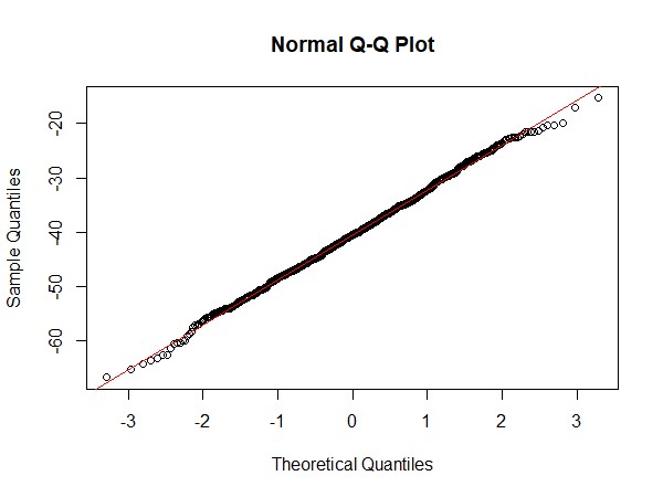
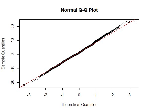
Figure 1. Q-Q plot of theoretical quantiles of normal distribution and sample quantiles from 1000 trials of $\tilde{v}_{nj}^{(0)}=\sqrt{n}\left(\tilde{\beta}^{\ast(0)}_{nj}-\beta_{0j}^{\ast}\right)$ for $j=1,2$. The estimators are generated with $n=500$ and $(\beta_{01},\beta_{02})=(5,0)$. This provides numerical evidence of normality for estimators of $\beta$ in model (1.1) with normal errors, although we have not theoretically guaranteed it.

4.3. Effect of iterations

Sparse and non-sparse parameters behave very differently under the AR scheme. Non-zero parameters are not expected to see apparent improvements in performance with added iterations, while estimates for the zero components will shrink as discussed in 3.9. As such, we present the numerical results separately below.

Sample densities of the 1000 independent estimates of $\alpha_{01}=2$ are shown on the left of Figure 2. The green line provides evidence of a normal density of the initial estimator, in line with 3.5. The three other lines for $k=2,5,10$ mostly overlap as there is no visible improvement in performance under more iterations. The empirical mean squared error (eMSE) of the initial estimator $\tilde{\alpha}_{n1}^{(0)}$ was $8.9\times 10^{-3}$ whereas the eMSE for $\tilde{\alpha}_{n1}^{(k)}$ for $k=2,5,10$ were reduced approximately $1.2\times 10^{-3}$, which is a result of re-weighting for non-homogeneous errors.

The initial estimator $\tilde{\beta}^{\ast(0)}_{n1}$ shows significant bias as seen in Figure 2 when estimating $\beta_{01}=5$. Upon iterating, bias is reduced due to more accurate plug-in estimators $\tilde{\alpha}_{n1}^{(k)}$ for (2.5). As in the case for $\alpha$, there is no major difference in performance between the cases $k=2,5,10$. The eMSE for $\tilde{\beta}^{\ast(0)}_{n1}$ was 3.41, and 0.354, 0.451 and 0.455 for $\tilde{\beta}^{\ast(2)}_{n1}$, $\tilde{\beta}^{\ast(5)}_{n1}$ and $\tilde{\beta}^{\ast(10)}_{n1}$ respectively.

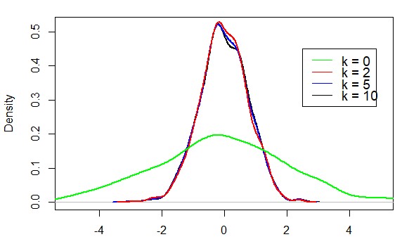
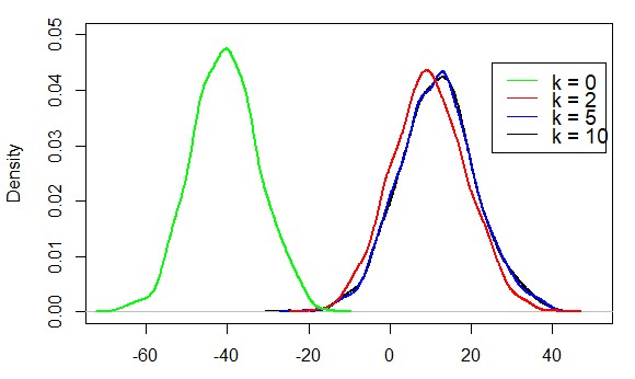
Figure 2. Sample densities of $\sqrt{n}\left(\tilde{\alpha}_{n1}^{(k)}-\alpha_{01}\right)$ (left) and $\sqrt{n}\left(\tilde{\beta}_{n1}^{\ast(k)}-\beta^{\ast}_{0}\right)$ (right) for $k=0,2,5,10$, $\alpha_{01}=2$ and $n=500$ over 1000 independent trials are shown on the left and right panels, respectively. These densities provide visualization of the AR estimators for non-sparse signals.

Next, we show the merits described by 3.6 and 3.9 when estimating sparse signals by numerically showing the shrinking effect to $\|\tilde{\alpha}_{n\circ}^{(k)}\|$ and $\|\tilde{\beta}_{n\circ}^{(k)}\|$ discussed in 3.9. In Table 1, we tabulated the medians of the absolute value of our 1000 estimates to show a central tendency towards $0$. The medians decrease as we perform more iterations, indicating that the estimates shrink, with the most notable drops being from $k=5$ to $k=10$ for all four estimators. We note that due to computational limitations, if more than half of the estimators are numerically 0, as in the cases of $\tilde{\alpha}_{n2}^{(10)}$ and $\tilde{\alpha}_{n3}^{(10)}$, then their medians will also be 0 even if their real values are non-zero.

Remark 4.1.

As we are considering large finite sample behaviour, it is possible that a few estimates for 0 components do not converge, but instead are much further away from $0$ than the rest. In such cases, if the mean was used to evaluate the extent of shrinkage, such outliers would prevent any meaningful comparison. Instead, by using the median, we do not need to worry about the discussed issue.

	$\tilde{\alpha}^{(k)}_{n2}$	$\tilde{\alpha}^{(k)}_{n3}$	$\tilde{\beta}^{(k)}_{n2}$	$\tilde{\beta}^{(k)}_{n3}$
$k=0$	0.068	0.077	0.22	0.21
$k=2$	$2\times 10^{-3}$	$2.9\times 10^{-3}$	0.049	0.052
$k=5$	$3.55\times 10^{-14}$	$1.53\times 10^{-12}$	$1.95\times 10^{-5}$	$1.27\times 10^{-5}$
$k=10$	0	0	$1.03\times 10^{-129}$	$2.76\times 10^{-132}$

Table 1. Medians of the absolute value of estimators $\tilde{\alpha}^{(k)}_{n2}$, $\tilde{\alpha}^{(k)}_{n3}$, $\tilde{\beta}^{(k)}_{n2}$ and $\tilde{\beta}^{(k)}_{n3}$ for zero parameters $\alpha_{02},\alpha_{03},\beta^{\ast}_{02}$ and $\beta^{\ast}_{03}$ are tabulated for $k=0,2,5,10$. The results are generated from 1000 independent trials with $n=500$.

We also provide histograms of estimates for $\tilde{\alpha}_{n2}^{(k)}$ and $\tilde{\beta}_{n2}^{(k)}$ ($k=0,2,5,10$) for a better picture of the shrinkage process in Figure 3 and Figure 4. We can also refer to the top-left ($k=0$) histograms for another observation of normality, which does not hold when $k\geq 1$. The histograms in Figure 3 and Figure 4 provide another perspective to shrinkage induced by the iteration scheme. Furthermore, we may refer to the top-left ($k=0$) histograms for extra empirical evidence of asymptotic normality under normal errors, which does not hold when $k\geq 1$.

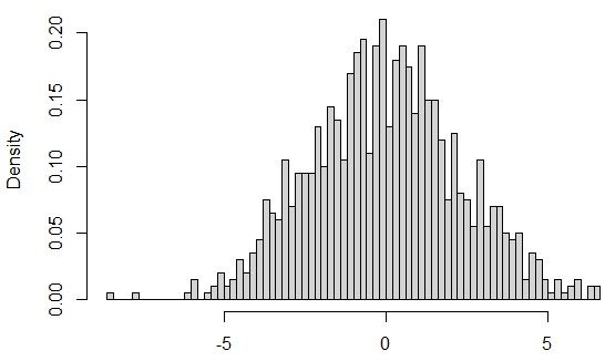
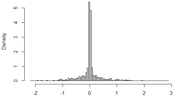
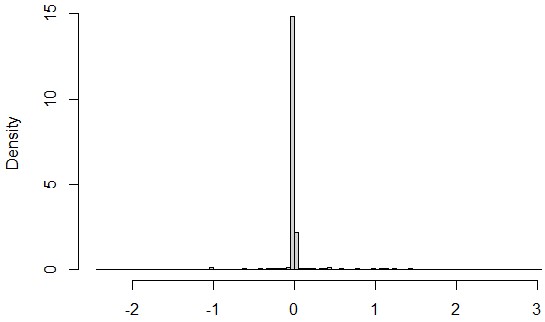
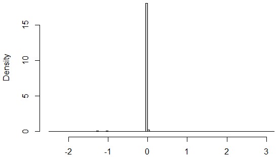
Figure 3. Histograms of $\sqrt{n}(\tilde{\alpha}_{n2}^{(k)}-\alpha_{02})$ for $k=0,2,5,10$ are shown. The histograms are ordered so that $k=0$ is on the top left, $k=2$ on the top right, $k=5$ on the bottom left, and $k=10$ on the bottom right. The true parameter is $\alpha_{02}=0$ and estimates are generated for $n=500$ with tuning matrix $\Lambda=I$, where $I$ is the identity matrix.

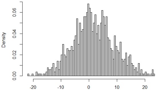
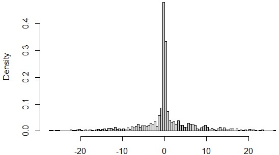
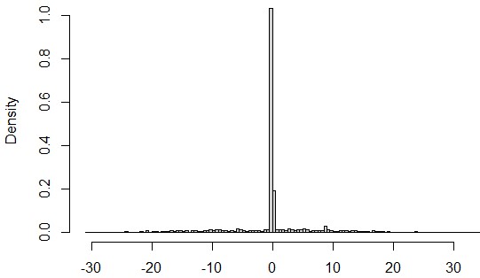
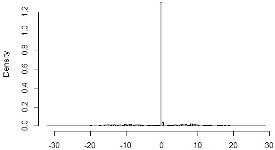
Figure 4. Histograms of $\sqrt{n}(\tilde{\alpha}_{n2}^{(k)}-\alpha_{02})$ for $k=0,2,5,10$ are shown. The histograms are ordered so that $k=0$ is on the top left, $k=2$ on the top right, $k=5$ on the bottom left, and $k=10$ on the bottom right. The true parameter is $\beta^{\ast}_{02}=0$ and estimates are generated for $n=500$ with tuning matrix $\Gamma^{\ast}=I$.

4.4. Model 2: Setup

The next model is used for discussing the effect small parameters have on AR estimators. In this section, we adopt a similar setup as Section 4.1. We change the true parameters to $\alpha_{0}=(0.1,0,0,\alpha_{04},...,\alpha_{0,50})\in\mathbb{R}^{50}$ and $\beta_{0}=(5,0.05,0,\beta_{04},...,\beta_{09})\in\mathbb{R}^{9}$, where the remaining components of $\alpha_{0}$ and $\beta_{0}$ are generated as $N(0,5^{2})$ and $N(0,1)$, and entries of $X$ and $Z$ are generated as $N(0,1)$ and $N(0,0.3^{2})$ independent random variables as before. In this section, we let $\Lambda=\lambda I$ and $\Gamma^{\ast}=\gamma I$ and change the values of $\lambda$ and $\gamma$ accordingly. We also change the distribution of $\epsilon_{1}$ to a $t$-distribution with degrees of freedom 2.5, whose main purpose is to incorporate a wider family of errors and suggest the possibility of weakening current assumptions on $\epsilon$. The result shows that our procedure continues to work under errors with heavier tails.

4.5. Presence of small parameters

While many sparse estimators usually provide desirable asymptotic results, their performances under finite samples can sometimes be overlooked. It is known that penalized schemes can suffer from inconsistency issues when small coefficients are present outside the asymptotic setting. See [13] for detailed analyses where they revealed weaknesses of the penalized estimator in a moving parameter setting by allowing the real parameter to perturb around $0$ at an order of $n^{-1/2}$. One of the strengths of the AR scheme is its flexibility in such scenarios. As both the magnitude of tuning parameters and the number of iterations $k$ can be adjusted, the degree of shrinkage can also be more properly and continuously controlled than most existing schemes.

The spikes away from 0 in Figure 5 correspond to estimates incorrectly shrunk towards 0. As the number of iterations increases, so does the frequency of this phenomenon. Away from the spike, the histograms are non-sparse, which is a reassuring sign of robustness against small parameters. Yet, the results are unsatisfactory especially for $k=5$ and $k=10$, as almost all estimates incorrectly interpreted a non-zero parameter as zero.

One approach to tackle this issue is to use smaller tuning parameters, which makes the scheme more sensitive to small parameters but reduces shrinkage. We show the results in Figure 6 reducing $\lambda$ from 1 to 0.1 and $\gamma$ from 1 to 0.001, where we also increase the number of iterations in return. In doing so, the frequency of incorrect shrinkage is drastically reduced, and the distribution for non-zero parameters is recovered even when $k$ is large. In particular, allowing for a trade-off of performance and computation efficiency is one of the merits of using the AR.

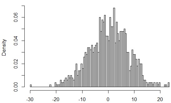
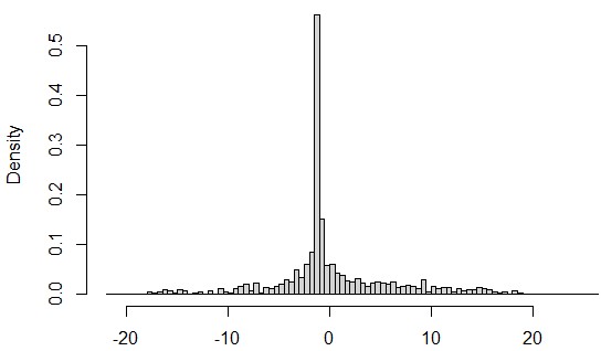
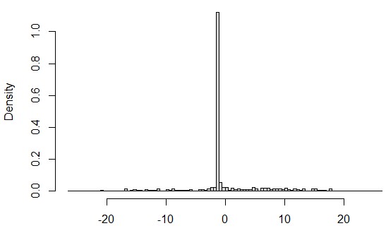
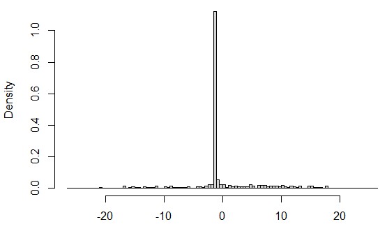
Figure 5. Incorrect shrinkage as a result of small parameters under the AR scheme are shown in the form of histograms of $\sqrt{n}(\tilde{\beta}_{n2}^{(k)}-\beta_{02})$ for $k=0,2,5,10$. The true signal is $\beta_{02}=0.05$ and estimates are generated with $n=500$ and tuning parameters $\lambda=\gamma=1$. The histograms are ordered so that $k=0$ is on the top left, $k=2$ on the top right, $k=5$ on the bottom left, and $k=10$ on the bottom right. The spikes in the cases of $k>0$ correspond to incorrect shrinkage towards 0.

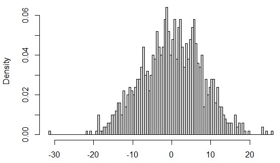
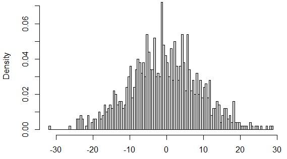
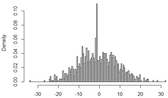
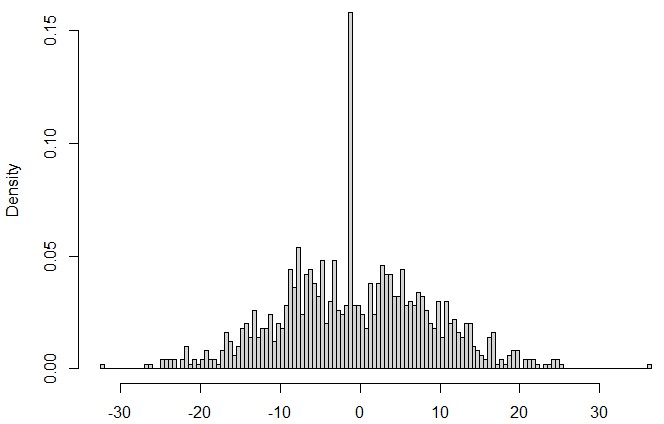
Figure 6. Incorrect shrinkage of small parameters under the AR scheme can be neutralized by setting smaller tuning parameters and increasing the number of iterations. The histograms of $\sqrt{n}(\tilde{\beta}_{n2}^{(k)}-\beta_{02})$ for $k=0,10,20,50$ are ordered so that $k=0$ is on the top left, $k=10$ on the top right, $k=20$ on the bottom left, and $k=50$ on the bottom right. The true signal is $\beta_{02}=0.05$ and the estimates are generated with $n=500$ and tuning parameters $\lambda=0.1$ and $\gamma=0.001$. Comparing these histograms with Figure 5 reveals the differences in performance.

5. Electricity Consumption Data Analysis

We analyze electricity consumption data obtained from Tokyo Electric Power Company Holdings, Incorporated (TEPCO) for 2018 to 2021 as a real-data example. The data is available on TEPCO’s official website (”https://www4.tepco.co.jp/en/forecast/html/download-e.html”) and contains records of the highest hourly consumption, contributing to a total of $(3\times 365+366)\times 24=35,064$ entries. We have split the data into training (2018 and 2019, $n=17020$) and testing (2020 and 2021, $n=17044$) sets.

$X$ and $Z$ contain 64 features, including the day of the week ($d$: Tuesday to Sunday), hour of day ($h^{m}$) and temperature ($t^{n}$), public holidays ($ph$), weekend public holidays ($wph$) and interaction terms ($h^{m}\times t^{n}$, $ph\times h^{m}$, $ph\times t^{n}$, $d\times h^{m}$), where $m,n\in\{1,2,3,4\}$. The design matrices have been standardized so that each column has mean 0 and unit variance, whereas the consumption data $Y$ has been centralized to have mean 0 for ease of calculations.

We compare the estimates of $\alpha$ for AR estimators for $k=2,5,10$ with the LASSO [14] and Elastic Net [15] with elastic net mixing parameter 0.5. The LASSO and Elastic Net were both implemented using the R package glmnet [4] and were optimized using 10-fold CV over 100 values of tuning parameters. To reduce complexity, we let the tuning parameters be identical, so that $\Lambda=\lambda I$ and $\Gamma^{\ast}=\gamma I$. We performed simultaneously five-fold cross validation for $\lambda$ and $\gamma$, trialing 25 points from $(10^{k_{1}},10^{k_{2}})$ for $k_{1}=3,4,5,6,7$ and $k_{2}=-2,-1,0,1,2$, and $(10^{5},10^{1})$ was optimal. We will also show the AR estimates of $\beta^{\ast}$. Finally, the threshold to round small estimates to 0 is set to be $10^{-4}$.

	LASSO	Elastic Net	AR ($k=2$)	AR ($k=5$)	AR ($k=10$)
ph	-33.0235	-36.2142	-62.3015	-45.0963	-50.0355
Tues	1.5724	-0.4790	-0.2587	0	0
Wed	7.7628	7.0601	-0.3479	0	0
Thurs	14.5631	9.4511	1.7723	0.0889	0
Fri	13.4204	14.5521	-3.2292	-4.1425	-0.0094
Sat	-89.3486	-89.4677	-105.9261	-83.6348	-61.0291
Sun	-138.9144	-127.5361	-94.2650	-115.6102	-94.6262
$t^{1}$	-653.5430	-515.4238	-610.9382	-881.6154	-898.8703
$t^{2}$	0	-348.0740	1.0840	0	0
$t^{3}$	788.1030	1108.7086	93.6917	1870.6414	1822.3644
$t^{4}$	0	-83.7872	746.4624	-956.4272	-900.4149
$h^{1}$	168.6433	265.2008	404.5176	-141.2085	-821.3668
…	…	…	…	…	…
Fri $\times$ $t^{1}$	-24.2677	-29.0486	0	0	0
Fri $\times$ $t^{2}$	0	0	0.0012	0	0
Fri $\times$ $t^{3}$	0	0	0.2434	0	0
Fri $\times$ $t^{4}$	31.5986	34.4185	13.4298	18.9116	20.4004
Sat $\times$ $t^{1}$	5.7711	28.2225	0	0	0
Sat $\times$ $t^{2}$	-3.9340	-38.7760	0.0230	0	0
Sat $\times$ $t^{3}$	0	0	0.1239	0	0
Sat $\times$ $t^{4}$	0	14.2698	0.6059	0	0
Sun $\times$ $t^{1}$	0	-32.9260	-94.0100	1.0281	0
Sun $\times$ $t^{2}$	19.7139	0	28.6261	-3.6234	0
Sun $\times$ $t^{3}$	0	114.2071	7.6010	-6.7407	-9.6121
Sun $\times$ $t^{4}$	-39.6542	-112.9375	-0.0340	0	0
Selected Predictors	40	57	60	36	26
MSPE	74425.05	73281.74	93358.09	78277.78	74487.11

Table 2. Table showing some of the estimated coefficients from the LASSO, Elastic Net, and AR $(k=2,5,10)$ schemes. The MSPE of the AR10 is very similar to optimized LASSO and Elastic Net algorithms. The number of selected predictors from the AR scheme also decreases with iterations.

	$k=2$	$k=5$	$k=10$
Intercept	9.9408	9.5954	9.4546
ph	-0.2105	-0.1197	-0.0017
Tues	-0.0075	0	0
Wed	-0.0131	-0.0002	0
Thurs	0	0	0
Fri	-0.1403	-0.0423	-0.0984
Sat	-0.2844	-0.1511	0
Sun	-0.3449	-0.1677	0
$t^{1}$	0.6288	-0.0123	0
$t^{2}$	-2.2129	-2.3932	-3.8494
Sat $\times$ $t^{1}$	0	0	0
Sat $\times$ $t^{2}$	0	0	0
Sat $\times$ $t^{3}$	0	0	0
Sat $\times$ $t^{4}$	-0.0151	-0.0008	0
Sun $\times$ $t^{1}$	0.0382	0	0
Sun $\times$ $t^{2}$	0.1866	0.0752	0.0868
Sun $\times$ $t^{3}$	-0.0798	0	0
Sun $\times$ $t^{4}$	0	0	0
Selected Predictors	57	36	20

Table 3. Table showing some of the estimated coefficients of $\tilde{\beta}^{\ast(2)}_{n}$, $\tilde{\beta}^{\ast(5)}_{n}$ and $\tilde{\beta}^{\ast(10)}_{n}$ using training data from 2018 to 2019 for 2, 5 and 10 iterations respectively. The AR scheme selects fewer predictors after the threshold is applied due to the shrinkage behavior discussed in 3.9.

Some of the estimated coefficients of $\alpha$ are shown in Table 2. Among the AR estimators, $\tilde{\alpha}_{n}^{(10)}$ (AR10) selects the fewest number of predictors and has minimal MSPE. The AR10 also shares similar performances to well-established and optimized schemes like the LASSO and Elastic Net. We refer to Figure 7 to visualize the fit of each of the estimators.

As shown in Table 2, the AR becomes increasingly sparse (post-threshold), as the number of selected predictors decreases with the number of iterations, as described in 3.9. Another feature to be noted is how the AR scheme preserves very small coefficients even for $k=10$. For instance, estimates such as $-0.0094$ are still preserved, as in the case of $(Fri)$ for $k=10$.

On the other hand, Table 3 shows the estimates for $\beta$. Results indicate the model might not be purely homogeneous, and the estimators have identified relevant features. Shrinkage is also observed here as the number of selected predictors drops with the number of iterations.

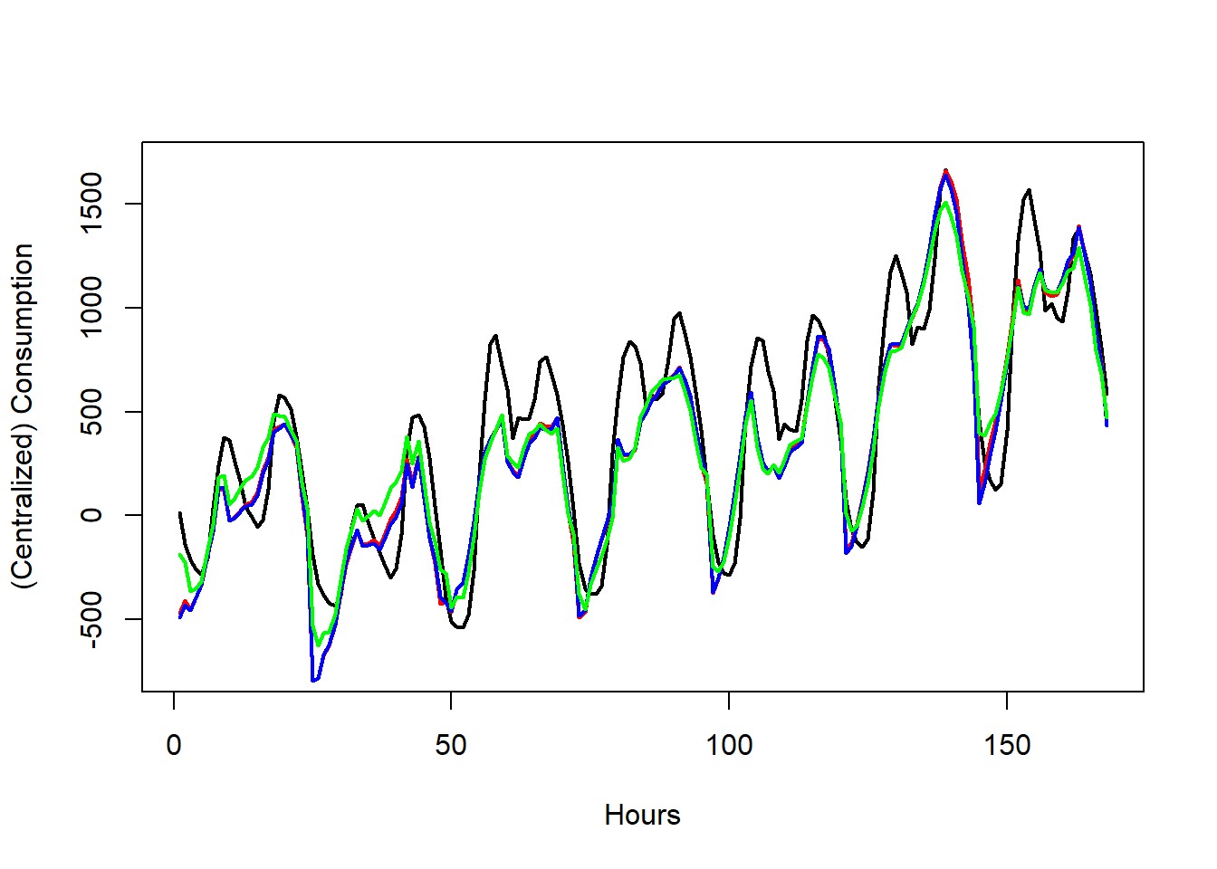
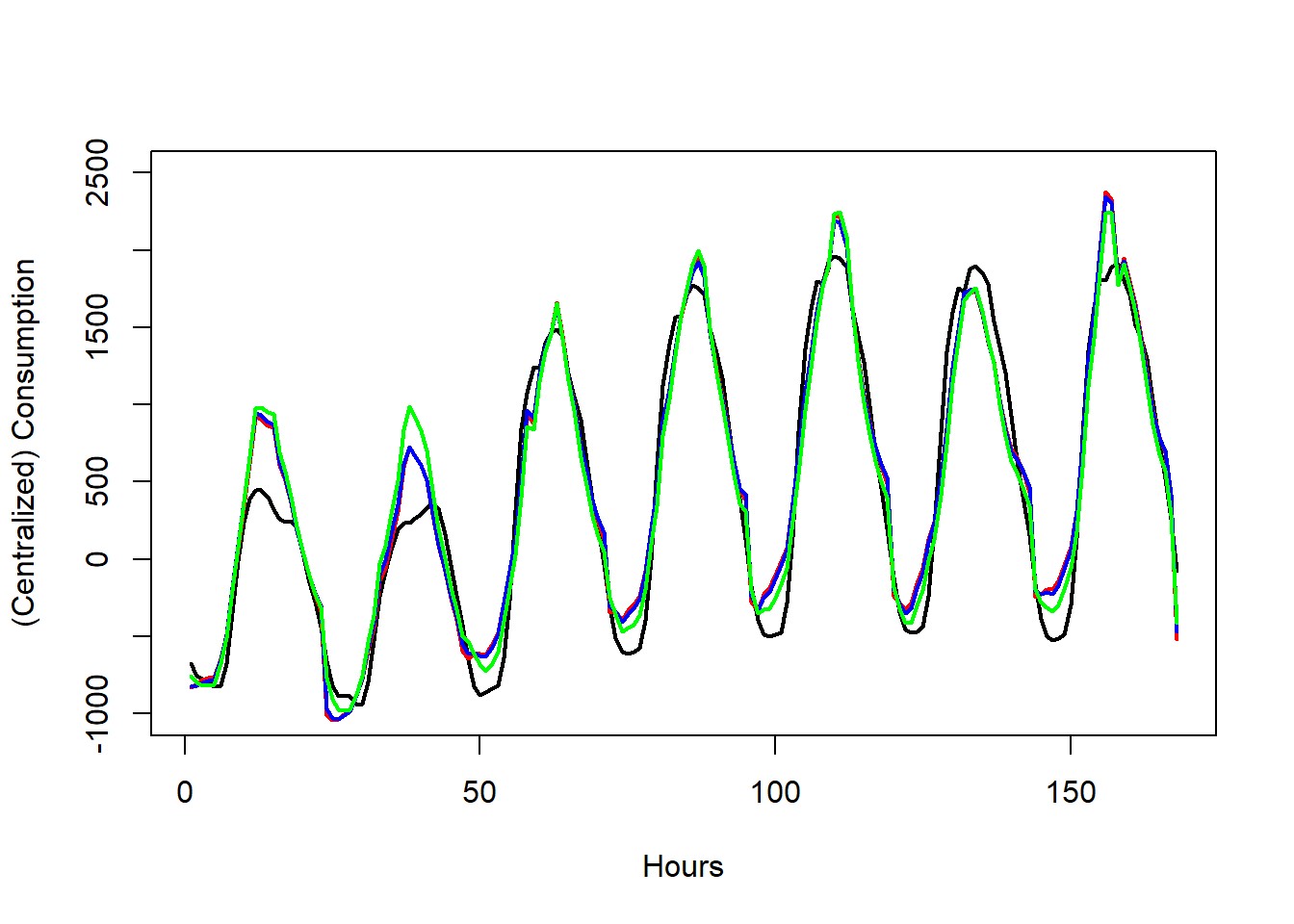
Figure 7. Figure shows predicted electricity consumption for a week (February 1 to February 7, 2020, LEFT) and a week in summer (August 1 to August 7, 2020, RIGHT) from the testing set. The AR10 (Adaptive Ridge with $k=10$, GREEN), LASSO (RED), and Elastic Net (BLUE) are compared with the true consumption (BLACK). Very similar levels of performance can be observed.

6. Discussion and Concluding Remarks

One area for future work is on extending the tuning matrices $\Lambda_{n}$ and $\Gamma^{\ast}_{n}$ to general positive definite matrices. We believe similar results should arise by generic eigenvalue arguments. On this avenue, improvement can also be made in the selection of tuning parameters.

Motivated by the numerical success in Section 4, it is likely that the assumptions on $\epsilon$ can be weakened so that asymptotic distributional results for $\beta^{\ast}$ hold under a wider class of errors. Further, to strengthen the result given in 3.6, one can attempt to construct approximate confidence sets for the iterated estimators of $k\geq 1$.

Finally, with the success of ordinary ridge estimators in high-dimensional settings, it will be interesting to see the AR as an extension of high-dimensional ridge regression. Alternatively, motivated by the success in modeling electricity consumption data, we are optimistic that the estimator can be generalized to other frameworks such as time series or stochastic differential equations.

Acknowledgement

The first author (KH) would like to thank JGMI of Kyushu University for their support. Also, this work was partially supported by JST CREST Grant Number JPMJCR2115 and JSPS KAKENHI Grant Number 22H01139, Japan (HM).

Appendix A Proof of 3.5

We begin by stating the matrix inversion formula (also known as the first-order resolvent formula or Sherman-Morrison-Woodbury formula), used as in [2]:

$$(X^{T}X+\Lambda_{n})^{-1}=(X^{T}X)^{-1}-(X^{T}X)^{-1}\Lambda_{n}(X^{T}X+\Lambda_{n})^{-1}.$$ (A.1)

Using (A.1), we write

$$\begin{split}\sqrt{n}(\tilde{\alpha}^{(0)}_{n}-\alpha_{0})&=\sqrt{n}\left[(X^{T}X+\Lambda_{n})^{-1}X^{T}Y-\alpha_{0}\right]\\ &=\sqrt{n}\left[\left((X^{T}X)^{-1}-(X^{T}X)^{-1}\Lambda_{n}(X^{T}X+\Lambda_{n})^{-1}\right)X^{T}(X\alpha_{0}+D_{n}(\beta_{0})\epsilon)-\alpha_{0}\right]\\ &=\left(\frac{X^{T}X}{n}\right)^{-1}\frac{1}{\sqrt{n}}X^{T}D_{n}(\beta_{0})\epsilon-\left(\frac{X^{T}X}{n}\right)^{-1}\frac{\Lambda_{n}}{\sqrt{n}}\left(\frac{X^{T}X}{n}+\frac{\Lambda_{n}}{n}\right)^{-1}\frac{X^{T}Y}{n}.\end{split}$$ (A.2)

Let us first consider term $\left(\frac{X^{T}X}{n}\right)^{-1}\frac{1}{\sqrt{n}}X^{T}D_{n}(\beta_{0})\epsilon$, where we can apply the Lindeberg Central Limit Theorem. By writing

$$\frac{1}{\sqrt{n}}X^{T}D_{n}(\beta_{0})\epsilon=\frac{1}{\sqrt{n}}\sum_{i=1}^{n}{e^{\frac{1}{2}Z_{i}\beta_{0}}X_{i}^{T}\epsilon_{i}},$$

the mean is computed as$\frac{1}{\sqrt{n}}\sum_{i=1}^{n}{\mathbb{E}\left[e^{\frac{1}{2}Z_{i}\beta_{0}}X_{i}^{T}\epsilon_{i}\right]}=0$, where $0$ denotes the $p$-dimensional $0$-vector. Also, the covariance

$$\frac{1}{n}\sum_{i=1}^{n}{{\rm cov}[e^{\frac{1}{2}Z_{i}\beta_{0}}X_{i}^{T}\epsilon_{i}}]=\frac{1}{n}\sum_{i=1}^{n}{e^{Z_{i}\beta_{0}}X_{i}^{T}X_{i}\mathbb{E}\left[\epsilon_{i}^{2}\right]}=\frac{X^{T}D^{2}_{n}(\beta_{0})X}{n}\to\Sigma^{X}_{+}$$

under 3.1. Finally, to check for Lindeberg’s condition, we let $m_{n}:=\max_{1\leq i\leq n}[\frac{e^{Z_{i}\beta_{0}}X_{i}X_{i}^{T}}{n}]$ and note that $m_{n}\to 0$ by 3.2. Thus for any $\delta>0$,

$$\frac{1}{n}\sum_{i=1}^{n}{\mathbb{E}\left[\|e^{\frac{1}{2}Z_{i}\beta_{0}}X_{i}^{T}\epsilon_{i}\|^{2};\|e^{\frac{1}{2}Z_{i}\beta_{0}}X_{i}^{T}\epsilon_{i}\|^{2}\geq n\delta\right]} =\sum_{i=1}^{n}{\frac{e^{Z_{i}\beta_{0}}X_{i}X_{i}^{T}}{n}\mathbb{E}\left[\epsilon_{i}^{2};\epsilon_{i}^{2}\geq\dfrac{\delta}{\frac{e^{Z_{i}\beta_{0}}X_{i}X_{i}^{T}}{n}}\right]}$$

$$\leq\mathbb{E}\left[\epsilon_{1}^{2};\epsilon_{1}^{2}>\frac{\delta}{m_{n}}\right]\sum_{i=1}^{n}{\frac{e^{Z_{i}\beta_{0}}X_{i}X_{i}^{T}}{n}}$$

$$={\rm tr}\left({\frac{X^{T}D_{n}^{2}(\beta_{0})X}{n}}\right)\mathbb{E}\left[\epsilon_{1}^{2};\epsilon_{1}^{2}>\frac{\delta}{m_{n}}\right]$$

$$\to 0,$$

where the final limit follows from $\frac{X^{T}D_{n}^{2}(\beta_{0})X}{n}\to\Sigma_{+}^{X}$ and applying Lebesgue’s Dominated Convergence Theorem on the sequence $\mathbb{E}\left[\epsilon_{1}^{2};\epsilon_{1}^{2}>\frac{\delta}{m_{n}}\right]$. Thus the first term of (A.2) converges in law:

$$\left(\frac{X^{T}X}{n}\right)^{-1}\frac{1}{\sqrt{n}}X^{T}D_{n}(\beta_{0})\epsilon\xrightarrow{\mathcal{L}}N\left(0,(\Sigma^{X})^{-1}\Sigma^{X}_{+}(\Sigma^{X})^{-1}\right).$$ (A.3)

As for the other term of the sum in (A.2), we rewrite it as

$$\left(\frac{X^{T}X}{n}\right)^{-1}\frac{\Lambda_{n}}{\sqrt{n}}\left(\frac{X^{T}X}{n}+\frac{\Lambda_{n}}{n}\right)^{-1}\frac{X^{T}Y}{n}=\left(\frac{X^{T}X}{n}\right)^{-1}\frac{\Lambda_{n}}{n}\left(\frac{X^{T}X}{n}+\frac{\Lambda_{n}}{n}\right)^{-1}\frac{1}{n}X^{T}\left(X\alpha_{0}+D_{n}(\beta_{0})\epsilon\right),$$

which we further evaluate as a sum of two terms. By (A.3) and $\frac{\Lambda_{n}}{\sqrt{n}}\to\Lambda_{0}$ ($\frac{\Lambda_{n}}{n}\to 0$), it follows that

$$\left(\frac{X^{T}X}{n}\right)^{-1}\frac{\Lambda_{n}}{\sqrt{n}}\left(\frac{X^{T}X}{n}+\frac{\Lambda_{n}}{n}\right)^{-1}\frac{1}{n}X^{T}D_{n}(\beta_{0})\epsilon\xrightarrow{p}0,$$

and

$$\left(\frac{X^{T}X}{n}\right)^{-1}\frac{\Lambda_{n}}{\sqrt{n}}\left(\frac{X^{T}X}{n}+\frac{\Lambda_{n}}{n}\right)^{-1}\frac{X^{T}X}{n}\alpha_{0}\to(\Sigma^{X})^{-1}\Lambda_{0}\alpha_{0}.$$

Combining these results with (A.3) show asymptotic normality as stated in (3.3):

$$\sqrt{n}(\tilde{\alpha}^{(0)}_{n}-\alpha_{0})\xrightarrow{\mathcal{L}}N\left(-(\Sigma^{X})^{-1}\Lambda_{0}\alpha_{0},(\Sigma^{X})^{-1}\Sigma^{X}_{+}(\Sigma^{X})^{-1}\right).$$

We now proceed to the asymptotics of $\tilde{\beta}^{\ast(0)}_{n}$. First note that

$$L_{n}(\alpha_{0}) =Z\beta_{0}+{\rm log}(\epsilon^{2})$$

$$=Z^{\ast}\beta^{\ast}_{0}+{\rm log}(\epsilon^{2})-\mathbb{E}\left[{\rm log}(\epsilon^{2})\right].$$

We denote $E_{n}:={\rm log}(\epsilon^{2})-\mathbb{E}\left[{\rm log}(\epsilon^{2})\right]$ and $R_{n}:=L_{n}(\tilde{\alpha}_{n}^{(0)})-L_{n}(\alpha_{0})$, so that for $c\in[0,\frac{1}{2})$,

$$\begin{split}n^{c}(\tilde{\beta}^{\ast(0)}_{n}-\beta^{\ast}_{0})&=n^{c}\left((Z^{\ast T}Z^{\ast}+\Gamma^{\ast}_{n})^{-1}Z^{\ast T}L_{n}(\tilde{\alpha}_{n}^{(0)})-\beta^{\ast}_{0}\right)\\ &=n^{c}\left[\left(\frac{Z^{\ast T}Z^{\ast}}{n}+\frac{\Gamma^{\ast}_{n}}{n}\right)^{-1}\frac{Z^{\ast T}Z^{\ast}\beta_{0}^{\ast}}{n}-\beta_{0}^{\ast}\right]+\left(\frac{Z^{\ast T}Z^{\ast}}{n}+\frac{\Gamma^{\ast}_{n}}{n}\right)^{-1}\frac{Z^{\ast T}E_{n}}{n^{1-c}}\\ &+\left(\frac{Z^{\ast T}Z^{\ast}}{n}+\frac{\Gamma^{\ast}_{n}}{n}\right)^{-1}\frac{Z^{\ast T}R_{n}}{n^{1-c}}.\end{split}$$ (A.4)

By (A.1), the first term of the sum vanishes as $n\to\infty$ for $c\leq\frac{1}{2}$ under $\frac{\Gamma^{\ast}_{n}}{\sqrt{n}}\to 0$:

$$n^{c}\left[\left(\frac{Z^{\ast T}Z^{\ast}}{n}+\frac{\Gamma^{\ast}_{n}}{n}\right)^{-1}\frac{Z^{\ast T}Z^{\ast}\beta_{0}^{\ast}}{n}-\beta_{0}^{\ast}\right]$$

$$= \text{ }n^{c}\left[\left(\frac{Z^{\ast T}Z^{\ast}}{n}\right)^{-1}\frac{Z^{\ast T}Z^{\ast}\beta_{0}^{\ast}}{n}-\left(\frac{Z^{\ast T}Z^{\ast}}{n}\right)^{-1}\frac{\Gamma^{\ast}_{n}}{n}\left(\frac{Z^{\ast T}Z^{\ast}}{n}+\frac{\Gamma^{\ast}_{n}}{n}\right)^{-1}\frac{Z^{\ast T}Z^{\ast}\beta_{0}^{\ast}}{n}-\beta_{0}^{\ast}\right]$$

$$= -\left(\frac{Z^{\ast T}Z^{\ast}}{n}\right)^{-1}\frac{\Gamma^{\ast}_{n}}{n^{1-c}}\left(\frac{Z^{\ast T}Z^{\ast}}{n}+\frac{\Gamma^{\ast}_{n}}{n}\right)^{-1}\frac{Z^{\ast T}Z^{\ast}\beta_{0}^{\ast}}{n}$$

$$\to \text{ }0.$$

Then, if we write $\frac{Z^{\ast T}E_{n}}{\sqrt{n}}=\sum_{i=1}^{n}{\frac{Z_{i}^{\ast T}E_{ni}}{\sqrt{n}}}$ and use the Lindeberg Central limit theorem analogously, we obtain under 3.1 and $\frac{\Gamma^{\ast}_{n}}{\sqrt{n}}\to 0$ that

$$\left(\frac{Z^{\ast T}Z^{\ast}}{n}\right)^{-1}\frac{Z^{\ast T}E_{n}}{\sqrt{n}}\xrightarrow{\mathcal{L}}N\left(0,(\Sigma^{Z^{\ast}})^{-1}{\rm var}[{\rm log}(\epsilon_{1}^{2})]\right),$$ (A.5)

which also proves that the second term of (A.4) is $\mathchoice{{\scriptstyle\mathcal{O}}}{{\scriptstyle\mathcal{O}}}{{\scriptscriptstyle\mathcal{O}}}{\scalebox{0.7}{$\scriptscriptstyle\mathcal{O}$}}_{p}(1)$ if $c<1/2$.

We will first prove (3.4), and to this end, we are going to show the tightness of the third term of $\eqref{eq7.4}$:

$$\left(\frac{Z^{\ast T}Z^{\ast}}{n}+\frac{\Gamma^{\ast}_{n}}{n}\right)^{-1}\frac{Z^{\ast T}R_{n}}{n^{1-c}}=\mathcal{O}_{p}(1).$$

By 3.1, it is sufficient to show

$$\frac{Z^{\ast T}R_{n}}{n^{1-c}}=\mathcal{O}_{p}(1).$$

We denote $\tilde{u}^{(0)}_{n}=\sqrt{n}(\tilde{\alpha}_{n}^{(0)}-\alpha_{0})$, $\tilde{r}_{ni}^{(0)}=\dfrac{X_{i}\tilde{u}^{(0)}_{n}}{e^{\frac{1}{2}Z_{i}\beta_{0}}\epsilon_{i}}$, and $\tilde{\psi}^{(0)}_{ni}={\rm log}\bigg{|}1-\frac{1}{\sqrt{n}}\tilde{r}_{ni}^{(0)}\bigg{|}$. Let $I(A)$ denote the indicator function of the event $A$. Then,

$$\begin{split}\frac{Z^{\ast T}R_{n}}{n}&=\frac{2}{n}\sum_{i=1}^{n}{Z^{\ast}_{i}\tilde{\psi}^{(0)}_{ni}}\\ &=\frac{2}{n}\sum_{i=1}^{n}{Z^{\ast}_{i}\tilde{\psi}^{(0)}_{ni}\left(I\bigg{(}\bigg{|}\frac{\tilde{r}_{ni}^{(0)}}{\sqrt{n}}\bigg{|}\leq\frac{1}{2}\bigg{)}+I\bigg{(}\bigg{|}\frac{\tilde{r}_{ni}^{(0)}}{\sqrt{n}}\bigg{|}>\frac{1}{2}\bigg{)}\right)}=:M_{1,n}+M_{2,n}.\end{split}$$ (A.6)

We first treat $M_{1,n}$. Since for all $s\in[0,1)$ and $u\in\mathbb{R}$, there exists some constant $C_{s}$ so that

$$\bigg{|}{\rm log}|1-u|\bigg{|}I\bigg{(}u\leq\frac{1}{2}\bigg{)}\leq C_{s}|u|^{s}.$$

Using this with $u=\frac{1}{\sqrt{n}}\tilde{r}_{ni}^{(0)}$ we get by 3.2

$$\left\|\frac{2}{n}\sum_{i=1}^{n}{Z^{\ast}_{i}\tilde{\psi}^{(0)}_{ni}I\bigg{(}\bigg{|}\frac{\tilde{r}_{ni}^{(0)}}{\sqrt{n}}\bigg{|}\leq\frac{1}{2}\bigg{)}}\right\|\leq\frac{2C_{s}\|Z^{\ast}\|}{n}\sum_{i=1}^{n}{\bigg{|}\frac{\tilde{r}_{ni}^{(0)}}{\sqrt{n}}\bigg{|}^{s}}\lesssim\frac{1}{n}\sum_{i=1}^{n}{\bigg{|}\frac{\tilde{r}_{ni}^{(0)}}{\sqrt{n}}\bigg{|}^{s}}.$$ (A.7)

The following Lemma is required next.

Lemma A.1.

There exists some $N$ such that for all $s^{\prime}>1$,

$$\sup_{n>N}\mathbb{E}\left[\left\|\sqrt{n}(\tilde{\alpha}_{n}^{(0)}-\alpha_{0})\right\|^{s}\right]<\infty.$$

Proof.

Splitting $\sqrt{n}\left(\tilde{\alpha}_{n}^{(0)}-\alpha_{0}\right)$ as (A.2), we have for $s^{\prime}>1$,

$$\mathbb{E}\left[\left\|\sqrt{n}\left(\tilde{\alpha}_{n}^{(0)}-\alpha_{0}\right)\right\|^{s^{\prime}}\right] \leq\mathbb{E}\left[\left\|\left(\frac{X^{T}X}{n}\right)^{-1}\frac{1}{\sqrt{n}}X^{T}D_{n}(\beta_{0})\epsilon\right\|^{s^{\prime}}\right]$$

$$+\mathbb{E}\left[\left\|\left(\frac{X^{T}X}{n}\right)^{-1}\frac{\Lambda_{n}}{\sqrt{n}}\left(\frac{X^{T}X}{n}+\frac{\Lambda_{n}}{n}\right)^{-1}\frac{1}{n}X^{T}D_{n}(\beta_{0})\epsilon\right\|^{s^{\prime}}\right]$$

$$+\mathbb{E}\left[\left\|\left(\frac{X^{T}X}{n}\right)^{-1}\frac{\Lambda_{n}}{\sqrt{n}}\left(\frac{X^{T}X}{n}+\frac{\Lambda_{n}}{n}\right)^{-1}\frac{X^{T}X}{n}\alpha_{0}\right\|^{s^{\prime}}\right].$$

The final term of the sum is non-random and so is finite for all $s^{\prime}$. Then, using Assumptions 3.1 and 3.2, we can also bound the first and second terms:

$$\mathbb{E}\left[\left\|\left(\frac{X^{T}X}{n}\right)^{-1}\frac{1}{\sqrt{n}}X^{T}D_{n}(\beta_{0})\epsilon\right\|^{s^{\prime}}\right]\lesssim\mathbb{E}\left[\left\|\frac{1}{\sqrt{n}}\sum_{i=1}^{n}\epsilon_{i}\right\|^{s^{\prime}}\right]$$

and

$$\mathbb{E}\left[\left\|\left(\frac{X^{T}X}{n}\right)^{-1}\frac{\Lambda_{n}}{\sqrt{n}}\left(\frac{X^{T}X}{n}+\frac{\Lambda_{n}}{n}\right)^{-1}\frac{1}{n}X^{T}D_{n}(\beta_{0})\epsilon\right\|^{s^{\prime}}\right]\lesssim\mathbb{E}\left[\left\|\frac{1}{n}\sum_{i=1}^{n}\epsilon_{i}\right\|^{s^{\prime}}\right].$$

Therefore, taking the supremum yields

$$\sup_{n>N}\mathbb{E}\left[\left\|\sqrt{n}\left(\tilde{\alpha}_{n}^{(0)}-\alpha_{0}\right)\right\|^{s^{\prime}}\right] \lesssim\sup_{n>N}\mathbb{E}\left[\left\|\frac{1}{\sqrt{n}}\sum_{i=1}^{n}\epsilon_{i}\right\|^{s^{\prime}}\right].$$

Finally, $\mathbb{E}\left[\|\epsilon_{1}\|^{s^{\prime}}\right]<\infty$ of 3.3 is sufficient for $\sup_{n>N}\mathbb{E}\left[\left\|\frac{1}{\sqrt{n}}\sum_{i=1}^{n}\epsilon_{i}\right\|^{s^{\prime}}\right]<\infty$ ([1], [3]). ∎

We will now estimate the upper bound in (A.7) using the Markov and Hölder inequalities: under Assumptions 3.2 and 3.3, for any positive constant $M$:

$$\begin{split}\sup_{n}\mathbb{P}\left[\frac{1}{n}\sum_{i=1}^{n}{\bigg{|}\frac{\tilde{r}_{ni}^{(0)}}{\sqrt{n}}\bigg{|}^{s}}>Mn^{-s/2}\right]&\leq\sup_{n}\mathbb{P}\left[\frac{1}{n}\sum_{i=1}^{n}\frac{\|\tilde{u}_{n}^{(0)}\|^{s}}{|\epsilon_{i}|^{s}}\gtrsim M\right]\\ &\lesssim\sup_{n}\frac{1}{n}\sum_{i=1}^{n}\mathbb{E}\left[\frac{\|\tilde{u}_{n}^{(0)}\|^{s}}{|\epsilon_{i}|^{s}}\right]\\ &\lesssim\frac{1}{M}\sup_{n}\mathbb{E}\left[\|\tilde{u}_{n}^{(0)}\|^{sa}\right]^{\frac{1}{a}}\mathbb{E}\left[|\epsilon_{1}|^{-sb}\right]^{\frac{1}{b}}\\ &\to 0\end{split}$$ (A.8)

as $M\to\infty$ by A.1, provided that we choose $a$ and $b$ such that $a^{-1}+b^{-1}=1$ and $sb<1$. Therefore,

$$M_{1,n}=\frac{2}{n}\sum_{i=1}^{n}{Z^{\ast}_{i}\tilde{\psi}^{(0)}_{ni}I\bigg{(}\bigg{|}\frac{\tilde{r}_{ni}^{(0)}}{\sqrt{n}}\bigg{|}\leq\frac{1}{2}\bigg{)}}=\mathcal{O}_{p}(n^{-\frac{s}{2}}).$$ (A.9)

We now turn our attention to $M_{2,n}$. Taking expectations, we have

$$\mathbb{E}\left[\left\|\frac{2}{n}\sum_{i=1}^{n}{Z^{\ast}_{i}\tilde{\psi}^{(0)}_{ni}I\bigg{(}\bigg{|}\frac{\tilde{r}_{ni}^{(0)}}{\sqrt{n}}\bigg{|}>\frac{1}{2}\bigg{)}}\right\|\right] \lesssim\frac{1}{n}\sum_{i=1}^{n}{\mathbb{E}\left[|\tilde{\psi}^{(0)}_{ni}|I\bigg{(}\bigg{|}\frac{\tilde{r}_{ni}^{(0)}}{\sqrt{n}}\bigg{|}>\frac{1}{2}\bigg{)}\right]}$$

$$\leq\frac{1}{n}\sum_{i=1}^{n}{\mathbb{E}\left[|\tilde{\psi}^{(0)}_{ni}|^{a}\right]^{\frac{1}{a}}\mathbb{P}\left[\left|\frac{\tilde{r}_{ni}^{(0)}}{\sqrt{n}}\right|>\frac{1}{2}\right]^{\frac{1}{b}}}$$

$$\leq\frac{1}{n}\left(\sup_{n}\sup_{i}\mathbb{E}\left[|\tilde{\psi}^{(0)}_{ni}|^{a}\right]^{\frac{1}{a}}\right)\sum_{i=1}^{n}{\mathbb{P}\left[\left|\frac{\tilde{r}_{ni}^{(0)}}{\sqrt{n}}\right|>\frac{1}{2}\right]^{\frac{1}{b}}},$$

where we chose the exponents $a,b>1$ $(1/a+1/b=1)$ independently of that in (A.8). We bound $\frac{1}{n}\sum_{i=1}^{n}{\mathbb{P}\left[\left|\frac{\tilde{r}_{ni}^{(0)}}{\sqrt{n}}\right|>\frac{1}{2}\right]^{\frac{1}{b}}}$ similar to (A.8). For any $t\in(s,1)$ there is some constant $C_{t}$ such that

$$\begin{split}\frac{1}{n}\sum_{i=1}^{n}{\mathbb{P}\left[\left|\frac{\tilde{r}_{ni}^{(0)}}{\sqrt{n}}\right|>\frac{1}{2}\right]^{\frac{1}{b}}}&=\frac{1}{n}\sum_{i=1}^{n}{\mathbb{P}\left[\left|\tilde{r}_{ni}^{(0)}\right|^{t}>2^{-t}n^{\frac{t}{2}}\right]^{\frac{1}{b}}}\\ &\leq\frac{1}{n}\sum_{i=1}^{n}{\mathbb{P}\left[\frac{\|\tilde{u}_{n}^{(0)}\|^{t}}{|\epsilon_{i}|^{t}}>C_{t}n^{\frac{t}{2}}\right]^{\frac{1}{b}}}\\ &\lesssim\frac{1}{n}\sum_{i=1}^{n}{n^{-\frac{t}{2b}}\mathbb{E}\left[\frac{\|\tilde{u}_{n}^{(0)}\|^{t}}{|\epsilon_{i}|^{t}}\right]^{\frac{1}{b}}}\\ &\lesssim n^{-\frac{t}{2b}}.\end{split}$$ (A.10)

By choosing $b$ and $t$ so that $b>1$ and $\frac{t}{b}=s$, we get consistent results with (A.9). Finally,

$$|\tilde{\psi}_{ni}^{(0)}|^{a} =\left|{\rm log}\bigg{|}\frac{e^{\frac{1}{2}Z_{i}\beta_{0}}\epsilon_{i}-X_{i}\frac{1}{\sqrt{n}}\tilde{u}_{n}^{(0)}}{e^{\frac{1}{2}Z_{i}\beta_{0}}\epsilon_{i}}\bigg{|}^{a}\right|$$

$$\leq\bigg{(}{\rm log}\bigg{|}e^{\frac{1}{2}Z_{i}\beta_{0}}\epsilon_{i}-X_{i}\frac{1}{\sqrt{n}}\tilde{u}_{n}^{(0)}\bigg{|}+{\rm log}|e^{\frac{1}{2}Z_{i}\beta_{0}}\epsilon_{i}|\bigg{)}^{a}$$

$$\lesssim\bigg{(}{\rm log}\bigg{|}e^{\frac{1}{2}Z_{i}\beta_{0}}\epsilon_{i}-X_{i}\frac{1}{\sqrt{n}}\tilde{u}_{n}^{(0)}\bigg{|}\bigg{)}^{a}+\bigg{(}{\rm log}|e^{\frac{1}{2}Z_{i}\beta_{0}}\epsilon_{i}|\bigg{)}^{a}$$

$$\lesssim\bigg{|}e^{\frac{1}{2}Z_{i}\beta_{0}}\epsilon_{i}-X_{i}\frac{1}{\sqrt{n}}\tilde{u}_{n}^{(0)}\bigg{|}^{a^{\prime}}+\bigg{|}e^{\frac{1}{2}Z_{i}\beta_{0}}\epsilon_{i}-X_{i}\frac{1}{\sqrt{n}}\tilde{u}_{n}^{(0)}\bigg{|}^{-a^{\prime}}+|e^{\frac{1}{2}Z_{i}\beta_{0}}\epsilon_{i}|^{a^{\prime}}+|e^{\frac{1}{2}Z_{i}\beta_{0}}\epsilon_{i}|^{-a^{\prime}}$$

for any $a^{\prime}\in(0,1)$. The last inequality follows from choosing a sufficiently small $l$ using the following bound: For all real $l>0$, there exists some constant $C_{l}$ such that for all $|u|\neq 0$

$$\bigg{|}{\rm log}|u|\bigg{|}\leq C_{l}(|u|^{l}+|u|^{-l}).$$

Taking expectation and supremum over $i$ and $n$, the first, third, and fourth terms are all finite under Assumptions 3.2 and 3.3. Finally for sufficiently large $N$, by 3.4 we have

$$\begin{split}&\sup_{n>N}\sup_{i}\mathbb{E}\left[\left|e^{\frac{1}{2}Z_{i}\beta_{0}}\epsilon_{i}-X_{i}\frac{1}{\sqrt{n}}\tilde{u}_{n}^{(0)}\right|^{-a^{\prime}}\right]<\infty,\end{split}$$ (A.11)

Along with (A.10), we obtain

$$M_{2,n}=\frac{2}{n}\sum_{i=1}^{n}{Z^{\ast}_{i}\tilde{\psi}^{(0)}_{ni}I\left(\left|\frac{\tilde{r}_{ni}^{(0)}}{\sqrt{n}}\right|>\frac{1}{2}\right)}=\mathcal{O}_{p}(n^{-\frac{s}{2}}).$$ (A.12)

Combining the results of (A.9) and (A.12) proves (3.4). If there exists $\tau>0$ such that $\mathbb{E}\left[|\epsilon_{1}|^{-(1+\tau)}\right]<\infty$, then in (A.8) we can instead allow $s=1$ and $b\leq 1+\tau$ to get $M_{1,n}=\mathchoice{{\scriptstyle\mathcal{O}}}{{\scriptstyle\mathcal{O}}}{{\scriptscriptstyle\mathcal{O}}}{\scalebox{0.7}{$\scriptscriptstyle\mathcal{O}$}}_{p}(n^{-\frac{1}{2}})$ in (A.9) and in (A.10) let $1<b<t\leq 1+\tau$ to obtain $M_{2,n}=\mathchoice{{\scriptstyle\mathcal{O}}}{{\scriptstyle\mathcal{O}}}{{\scriptscriptstyle\mathcal{O}}}{\scalebox{0.7}{$\scriptscriptstyle\mathcal{O}$}}_{p}(n^{-\frac{1}{2}})$, which show $\left(\frac{Z^{\ast T}Z^{\ast}}{n}+\frac{\Gamma^{\ast}_{n}}{n}\right)^{-1}\frac{Z^{\ast T}R_{n}}{n^{1/2}}\to 0$ in (A.4). Finally, we deduce (3.5) using (A.5).

Appendix B Proof of 3.6

First, we write

$$\sqrt{n}(\tilde{\alpha}_{n}^{(1)}-\alpha_{0})$$

$$= \sqrt{n}\left(\left(\frac{X^{T}D_{n}^{-2}(\tilde{\beta}_{n}^{(0)})X}{n}+\Lambda_{n}\frac{T(\tilde{\alpha}_{n}^{(0)})}{n}\right)^{-1}\frac{1}{n}X^{T}D_{n}^{-2}(\tilde{\beta}_{n}^{(0)})Y-\alpha_{0}\right)$$

$$= \sqrt{n}\left(\left(\tilde{\Sigma}_{n-}^{(0)}+\Lambda_{n}\frac{T(\tilde{\alpha}_{n}^{(0)})}{n}\right)^{-1}\tilde{\Sigma}_{n-}^{(0)}\alpha_{0}-\alpha_{0}\right)+\left(\tilde{\Sigma}_{n-}^{(0)}+\Lambda_{n}\frac{T(\tilde{\alpha}_{n}^{(0)})}{n}\right)^{-1}\frac{1}{\sqrt{n}}X^{T}D_{n}^{-2}(\tilde{\beta}_{n}^{(0)})D_{n}(\beta_{0})\epsilon$$

$$\equiv I_{1,n}+I_{2,n},$$

where we denote $\tilde{\Sigma}_{n-}^{(0)}=\frac{X^{T}D_{n}^{-2}(\tilde{\beta}_{n}^{(0)})X}{n}$. We will first prove $I_{1,n}\xrightarrow{p}0$ and then simplify the expression of $I_{2,n}$.

Firstly, if no entries are exactly 0 then $I_{1,n}\xrightarrow{p}0$ follows from the consistency of $\tilde{\beta}_{n}^{(0)}$, $\Lambda_{n}\frac{T(\tilde{\alpha}_{n}^{(0)})}{\sqrt{n}}\xrightarrow{p}0$ and the matrix inversion formula, which is similar to what we have proved in 3.5. Otherwise, suppose $p_{0}<p$ are non-zero (The case where $p_{0}=0$ is similar to the result below without needing to consider block matrices), in which case we let

$$M =\left(\frac{X^{T}D_{n}^{-2}(\tilde{\beta}_{n}^{(0)})X}{n}+\Lambda_{n}\frac{T(\tilde{\alpha}_{n}^{(0)})}{n}\right)$$

$$=\left(\tilde{\Sigma}_{n-}^{(0)}+\Lambda_{n}\frac{T(\tilde{\alpha}_{n}^{(0)})}{n}\right)$$

$$=\begin{pmatrix}(\tilde{\Sigma}_{n-}^{(0)})_{\star\star}+\Lambda_{n}\frac{T_{\star}(\tilde{\alpha}_{n}^{(0)})}{n}&(\tilde{\Sigma}_{n-}^{(0)})_{\star\circ}\\ (\tilde{\Sigma}_{n-}^{(0)T})_{\star\circ}&(\tilde{\Sigma}_{n-}^{(0)})_{\circ\circ}+\Lambda_{n}\frac{T_{\circ}(\tilde{\alpha}_{n}^{(0)})}{n}\end{pmatrix}$$

$$=:\begin{pmatrix}A&B\\ B^{T}&D\\ \end{pmatrix}.$$

The Schur complement of $M$ is given by

$$S :=D-B^{T}A^{-1}B$$

$$=\left((\tilde{\Sigma}_{n-}^{(0)})_{\circ\circ}+\Lambda_{n}\frac{T_{\circ}(\tilde{\alpha}_{n}^{(0)})}{n}\right)-(\tilde{\Sigma}_{n-}^{(0)})_{\star\circ}\left((\tilde{\Sigma}_{n-}^{(0)})_{\star\star}+\Lambda_{n}\frac{T_{\star}(\tilde{\alpha}_{n}^{(0)})}{n}\right)^{-1}(\tilde{\Sigma}_{n-}^{(0)})_{\star\circ},$$

and the inverse of $M$ is [12]

$$M^{-1}=\begin{pmatrix}M^{-1}_{\star\star}&M^{-1}_{\star\circ}\\ (M^{-1}_{\star\circ})^{T}&M^{-1}_{\circ\circ}\end{pmatrix}=\begin{pmatrix}A^{-1}+A^{-1}BS^{-1}B^{T}A^{-1}&-A^{-1}BS^{-1}\\ -S^{-1}B^{T}A^{-1}&S^{-1}\end{pmatrix}.$$ (B.1)

Here, the matrices $(A,B,D,M,S)=(A_{n},B_{n},D_{n},M_{n},S_{n})$ are written without the subscript $n$ for brevity. Next, we rewrite $\frac{1}{\sqrt{n}}I_{1,n}$ as follows:

$$\begin{split}\frac{1}{\sqrt{n}}I_{1,n}=\frac{1}{\sqrt{n}}\begin{pmatrix}I_{1,n}^{\prime}\\ I_{1,n}^{\prime\prime}\end{pmatrix}&=M^{-1}\tilde{\Sigma}_{n-}^{(0)}\alpha_{0}-\alpha_{0}\\ &=\begin{pmatrix}M^{-1}_{\star\star}&M^{-1}_{\star\circ}\\ (M^{-1}_{\star\circ})^{T}&M^{-1}_{\circ\circ}\end{pmatrix}\begin{pmatrix}(\tilde{\Sigma}_{n-}^{(0)})_{\star\star}&(\tilde{\Sigma}_{n-}^{(0)})_{\star\circ}\\ (\tilde{\Sigma}_{n-}^{(0)})_{\star\circ}^{T}&(\tilde{\Sigma}_{n-}^{(0)})_{\circ\circ}\end{pmatrix}\begin{pmatrix}\alpha_{0\star}\\ 0\end{pmatrix}-\alpha_{0}\\ &=\begin{pmatrix}(M^{-1}_{\star\star}(\tilde{\Sigma}_{n-}^{(0)})_{\star\star}+M^{-1}_{\star\circ}(\tilde{\Sigma}_{n-}^{(0)})_{\star\circ}^{T})\alpha_{0\star}\\ \left((M^{-1}_{\star\circ})^{T}(\tilde{\Sigma}_{n-}^{(0)})_{\star\star}+M^{-1}_{\circ\circ}(\tilde{\Sigma}_{n-}^{(0)})_{\star\circ}^{T}\right)\alpha_{0\star}\end{pmatrix}-\begin{pmatrix}\alpha_{0\star}\\ 0\end{pmatrix}.\end{split}$$ (B.2)

We will proceed to evaluate the limits of the rows

$\left(M^{-1}_{\star\star}(\tilde{\Sigma}_{n-}^{(0)})_{\star\star}+M^{-1}_{\star\circ}(\tilde{\Sigma}_{n-}^{(0)})_{\star\circ}^{T}\right)\alpha_{0\star}-\alpha_{0\star}$

and

$\left((M^{-1}_{\star\circ})^{T}(\tilde{\Sigma}_{n-}^{(0)})_{\star\star}+M^{-1}_{\circ\circ}(\tilde{\Sigma}_{n-}^{(0)})_{\star\circ}^{T}\right)\alpha_{0\star}$

separately. For the upper part ($I_{1,n}^{\prime}$), note that $(\tilde{\Sigma}_{n-}^{(0)})_{\star\circ}=B$, so by (B.1) we get

$$\begin{split}M^{-1}_{\star\star}(\tilde{\Sigma}_{n-}^{(0)})_{\star\star}+M^{-1}_{\star\circ}(\tilde{\Sigma}_{n-}^{(0)})_{\star\circ}^{T}&=(A^{-1}+A^{-1}BS^{-1}B^{T}A^{-1})(\tilde{\Sigma}_{n-}^{(0)})_{\star\star}-A^{-1}BS^{-1}B^{T}\\ &=A^{-1}(\tilde{\Sigma}_{n-}^{(0)})_{\star\star}+A^{-1}BS^{-1}B^{T}(A^{-1}(\tilde{\Sigma}_{n-}^{(0)})_{\star\star}-I_{p_{0}}).\end{split}$$ (B.3)

Moreover by (A.1), since $\Lambda_{n}\frac{T_{\star}(\tilde{\alpha}_{n}^{(0)})}{n}=\mathchoice{{\scriptstyle\mathcal{O}}}{{\scriptstyle\mathcal{O}}}{{\scriptscriptstyle\mathcal{O}}}{\scalebox{0.7}{$\scriptscriptstyle\mathcal{O}$}}_{p}(1)$,

$$A^{-1}(\tilde{\Sigma}_{n-}^{(0)})_{\star\star}=\left((\tilde{\Sigma}_{n-}^{(0)})_{\star\star}+\Lambda_{n}\frac{T_{\star}(\tilde{\alpha}_{n}^{(0)})}{n}\right)^{-1}(\tilde{\Sigma}_{n-}^{(0)})_{\star\star}=I_{p_{0}}+\mathcal{O}_{p}\left(\frac{1}{n}\right).$$ (B.4)

Finally by 3.1, $\|B\|$ is bounded for large enough $n$, and since $\|A^{-1}\|\leq\left\|\left(\tilde{\Sigma}_{n-}^{(0)}\right)^{-1}\right\|$, $\|A^{-1}\|$ is bounded for all large enough $n$. Also, $\|M^{-1}\|\leq K_{X}$ so $\|S^{-1}\|$ is also bounded for all sufficiently large $n$, which jointly imply

$$A^{-1}BS^{-1}B^{T}=\mathcal{O}_{p}(1).$$

Therefore,

$$M^{-1}_{\star\star}(\tilde{\Sigma}_{n-}^{(0)})_{\star\star}+M^{-1}_{\star\circ}(\tilde{\Sigma}_{n-}^{(0)})_{\star\circ}^{T}=I_{p_{0}}+\mathcal{O}_{p}\left(\frac{1}{n}\right),$$

and thus

$$\sqrt{n}\left((M^{-1}_{\star\star}(\tilde{\Sigma}_{n-}^{(0)})_{\star\star}+M^{-1}_{\star\circ}(\tilde{\Sigma}_{n-}^{(0)})_{\star\circ}^{T})\alpha_{0\star}-\alpha_{0\star}\right)\xrightarrow{p}0.$$ (B.5)

For the second row ($I_{1,n}^{\prime\prime}$), we get

$$\begin{split}(M^{-1}_{\star\circ})^{T}(\tilde{\Sigma}_{n-}^{(0)})_{\star\star}+M^{-1}_{\circ\circ}(\tilde{\Sigma}_{n-}^{(0)})_{\star\circ}^{T}&=-S^{-1}B^{T}A^{-1}(\tilde{\Sigma}_{n-}^{(0)})_{\star\star}+S^{-1}(\tilde{\Sigma}_{n-}^{(0)})_{\star\circ}^{T}\\ &=S^{-1}B^{T}(I_{p_{0}}-A^{-1}(\tilde{\Sigma}_{n-}^{(0)})_{\star\star})\\ &=S^{-1}B^{T}\left(I_{p_{0}}-I_{p_{0}}+\mathcal{O}_{p}\left(\frac{1}{n}\right)\right)\\ &=\mathcal{O}_{p}\left(\frac{1}{n}\right).\end{split}$$ (B.6)

Therefore,

$$\sqrt{n}\left((M^{-1}_{\star\circ})^{T}(\tilde{\Sigma}_{n-}^{(0)})_{\star\star}+M^{-1}_{\circ\circ}(\tilde{\Sigma}_{n-}^{(0)})_{\star\circ}^{T}\right)\alpha_{0\star}\xrightarrow{p}0.$$ (B.7)

Substituting (B.5) and (B.7) into (B.2) gives

$I_{1,n}=\mathchoice{{\scriptstyle\mathcal{O}}}{{\scriptstyle\mathcal{O}}}{{\scriptscriptstyle\mathcal{O}}}{\scalebox{0.7}{$\scriptscriptstyle\mathcal{O}$}}_{p}(1)$

as required.

Moving onto $I_{2,n}$, the consistency of $\tilde{\beta}_{n}^{(0)}$ and $\|Z_{i}^{\ast}\|<\infty$ (3.2) imply

$$\max_{1\leq i\leq n}|e^{-Z_{i}\beta_{0}}-e^{-Z_{i}\tilde{\beta}_{n}^{(0)}}|\xrightarrow{p}0,$$

$$\tilde{\Sigma}_{n-}^{(0)}-\frac{X^{T}D^{-2}_{n}(\beta_{0})X}{n}\xrightarrow{p}0$$

and

$$X^{T}D_{n}^{-2}(\tilde{\beta}_{n}^{(0)})D_{n}(\beta_{0})\epsilon-X^{T}D_{n}^{-1}(\beta_{0})\epsilon\xrightarrow{p}0.$$

Writing $\Pi^{X}_{n}\coloneqq\frac{1}{\sqrt{n}}X^{T}D_{n}^{-1}(\beta_{0})\epsilon$ then gives

$$\begin{split}I_{2,n}&=\left(\tilde{\Sigma}_{n-}^{(0)}+\Lambda_{n}\frac{T(\tilde{\alpha}_{n}^{(0)})}{n}\right)^{-1}\frac{1}{\sqrt{n}}X^{T}D_{n}^{-2}(\tilde{\beta}_{n}^{(0)})D_{n}(\beta_{0})\epsilon\\ &=\left(\frac{X^{T}D^{-2}_{n}(\beta_{0})X}{n}+\Lambda_{n}\frac{T(\tilde{\alpha}_{n}^{(0)})}{n}\right)^{-1}\Pi^{X}_{n}+\mathchoice{{\scriptstyle\mathcal{O}}}{{\scriptstyle\mathcal{O}}}{{\scriptscriptstyle\mathcal{O}}}{\scalebox{0.7}{$\scriptscriptstyle\mathcal{O}$}}_{p}(1).\end{split}$$ (B.8)

We can use the Lindeberg CLT analogously as we did for (A.3) to obtain

$$\Pi^{X}_{n}\xrightarrow{\mathcal{L}}N(0,\Sigma_{-}^{X}).$$

Further, by noting $\left(\frac{X^{T}D^{-2}_{n}(\beta_{0})X}{n}-\Sigma_{-}^{X}\right)=\mathchoice{{\scriptstyle\mathcal{O}}}{{\scriptstyle\mathcal{O}}}{{\scriptscriptstyle\mathcal{O}}}{\scalebox{0.7}{$\scriptscriptstyle\mathcal{O}$}}(1)$ and $\Lambda_{n}\frac{T(\tilde{\alpha}_{n}^{(0)})}{n}-\begin{pmatrix}0&0\\ 0&\Lambda_{0\circ}T_{\circ}(\tilde{u}_{n}^{(0)})\end{pmatrix}=\mathchoice{{\scriptstyle\mathcal{O}}}{{\scriptstyle\mathcal{O}}}{{\scriptscriptstyle\mathcal{O}}}{\scalebox{0.7}{$\scriptscriptstyle\mathcal{O}$}}_{p}(1)$, we may appeal to (A.1) and $\Pi_{n}^{X}=\mathcal{O}_{p}(1)$ to conclude

$$\left(\frac{X^{T}D^{-2}_{n}(\beta_{0})X}{n}+\Lambda_{n}\frac{T(\tilde{\alpha}_{n}^{(0)})}{n}\right)^{-1}\Pi^{X}_{n}$$

$$= \left(\Sigma_{-}^{X}+\begin{pmatrix}0&0\\ 0&\Lambda_{0\circ}T_{\circ}(\tilde{u}_{n}^{(0)})\end{pmatrix}+\left(\frac{X^{T}D^{-2}_{n}(\beta_{0})X}{n}-\Sigma_{-}^{X}\right)+\left(\Lambda_{n}\frac{T(\tilde{\alpha}_{n}^{(0)})}{n}-\begin{pmatrix}0&0\\ 0&\Lambda_{0\circ}T_{\circ}(\tilde{u}_{n}^{(0)})\end{pmatrix}\right)\right)^{-1}\Pi^{X}_{n}$$

$$= \left(\Sigma_{-}^{X}+\begin{pmatrix}0&0\\ 0&\Lambda_{0\circ}T_{\circ}(\tilde{u}_{n}^{(0)})\end{pmatrix}\right)^{-1}\Pi^{X}_{n}+\mathchoice{{\scriptstyle\mathcal{O}}}{{\scriptstyle\mathcal{O}}}{{\scriptscriptstyle\mathcal{O}}}{\scalebox{0.7}{$\scriptscriptstyle\mathcal{O}$}}_{p}(1).$$

Returning to (B.8), we obtain

$$\begin{split}I_{2,n}&=\left(\frac{X^{T}D^{-2}_{n}(\beta_{0})X}{n}+\Lambda_{n}\frac{T(\tilde{\alpha}_{n}^{(0)})}{n}\right)^{-1}\Pi^{X}_{n}+\mathchoice{{\scriptstyle\mathcal{O}}}{{\scriptstyle\mathcal{O}}}{{\scriptscriptstyle\mathcal{O}}}{\scalebox{0.7}{$\scriptscriptstyle\mathcal{O}$}}_{p}(1)\\ &=\left(\Sigma_{-}^{X}+\begin{pmatrix}0&0\\ 0&\Lambda_{0\circ}T_{\circ}(\tilde{u}_{n}^{(0)})\end{pmatrix}\right)^{-1}\Pi^{X}_{n}+\mathchoice{{\scriptstyle\mathcal{O}}}{{\scriptstyle\mathcal{O}}}{{\scriptscriptstyle\mathcal{O}}}{\scalebox{0.7}{$\scriptscriptstyle\mathcal{O}$}}_{p}(1),\end{split}$$ (B.9)

which proves (3.8).

We now move on to prove the corresponding results for $\tilde{\beta}^{\ast(1)}_{n}$ by first writing

$$\tilde{\beta}_{n}^{\ast(1)}-\beta^{\ast}_{0} =\left(\frac{Z^{\ast T}Z^{\ast}}{n}+\Gamma^{\ast}_{n}\frac{S(\tilde{\beta}^{\ast(0)}_{n})}{n}\right)^{-1}\frac{1}{n}Z^{\ast T}L_{n}(\tilde{\alpha}_{n}^{(1)})-\beta^{\ast}_{0}$$

$$=\left[\left(\frac{Z^{\ast T}Z^{\ast}}{n}+\Gamma^{\ast}_{n}\frac{S(\tilde{\beta}^{\ast(0)}_{n})}{n}\right)^{-1}\frac{Z^{\ast T}Z^{\ast}}{n}\beta^{\ast}_{0}-\beta^{\ast}_{0}\right]$$

$$+\left(\frac{Z^{\ast T}Z^{\ast}}{n}+\Gamma^{\ast}_{n}\frac{S(\tilde{\beta}^{\ast(0)}_{n})}{n}\right)^{-1}\frac{1}{n}Z^{\ast T}E_{n}+\left(\frac{Z^{\ast T}Z^{\ast}}{n}+\Gamma^{\ast}_{n}\frac{S(\tilde{\beta}^{\ast(0)}_{n})}{n}\right)^{-1}\frac{1}{n}Z^{\ast T}R_{n}^{(1)}$$

$$\equiv J_{1,n}+J_{2,n}+J_{3,n},$$

where

$R_{n}^{(1)}:=L(\tilde{\alpha}^{(1)}_{n})-L_{n}(\alpha_{0})$.

The term $J_{1,n}$ can be shown to be $\mathchoice{{\scriptstyle\mathcal{O}}}{{\scriptstyle\mathcal{O}}}{{\scriptscriptstyle\mathcal{O}}}{\scalebox{0.7}{$\scriptscriptstyle\mathcal{O}$}}_{p}(\frac{1}{\sqrt{n}})$ in the exact same way we did for $I_{1,n}$, swapping out $\tilde{\Sigma}_{n-}^{(0)}$ for $\frac{Z^{\ast T}Z^{\ast}}{n}$; $\Lambda_{n}$ for $\Gamma_{n}^{\ast}$; $\tilde{\alpha}_{n}^{(0)}$ for $\tilde{\beta}^{\ast(0)}_{n}$ and $\alpha_{0}$ for $\beta^{\ast}_{0}$. Then under 3.3, we denote $\Pi_{n}^{Z}\coloneqq\frac{1}{\sqrt{n}}Z^{\ast T}E_{n}$ and use the Lindeberg CLT to show

$$\Pi_{n}^{Z}\xrightarrow{\mathcal{L}}N\left(0,\Sigma^{Z^{\ast}}{\rm var}[{\rm log}(\epsilon_{1}^{2})]\right),$$

which also implies $J_{2,n}=O_{p}(\frac{1}{\sqrt{n}})$.

Finally, under B.1 (stated below), we can follow the proof of 3.5 to show that $J_{3,n}=O_{p}(n^{-\frac{c}{2}})$ for all $c\in(0,1)$ by bounding the term $\frac{1}{n}Z^{\ast T}R_{n}^{(1)}$, which gives (3.9). Further, with the stronger condition of $\mathbb{E}\left[|\epsilon_{1}|^{-(1+\tau)}\right]<\infty$ for some $\tau>0$, we can proceed as in (B.9) to get

$$\sqrt{n}J_{2,n} =\left(\frac{Z^{\ast T}Z^{\ast}}{n}+\Gamma^{\ast}_{n}\frac{S(\tilde{\beta}^{\ast(0)}_{n})}{n}\right)^{-1}\Pi_{n}^{Z}$$

$$=\left(\Sigma^{Z^{\ast}}+\begin{pmatrix}0&0\\ 0&\Gamma_{0\circ}^{\ast}S_{\circ}(v_{n}^{(0)})\end{pmatrix}\right)^{-1}\Pi_{n}^{Z}+\mathchoice{{\scriptstyle\mathcal{O}}}{{\scriptstyle\mathcal{O}}}{{\scriptscriptstyle\mathcal{O}}}{\scalebox{0.7}{$\scriptscriptstyle\mathcal{O}$}}_{p}(1),$$

which gives (3.10). The statement for general $k\geq 2$ follows inductively.

We state a similar Lemma as A.1 to prove corresponding results for $\tilde{\beta}^{\ast(k)}_{n}$.

Lemma B.1.

For each $k\geq 1$, there exists some $N$ such that for all $s>1$,

$$\sup_{n>N}\mathbb{E}\left[\left\|\sqrt{n}(\tilde{\alpha}_{n}^{(k)}-\alpha_{0})\right\|^{s}\right]<\infty.$$

Proof.

We only consider $k=1$ as the general case follows the same proof. We write $\sqrt{n}(\tilde{\alpha}_{n}^{(1)}-\alpha_{0})=I_{1,n}+I_{2,n}$ as before, and we will bound the moments of each of the two terms.

Using the same notation as in (B.2), we may write $I_{1,n}$ as follows and bound the upper and lower parts separately:

$$\begin{split}I_{1,n}&=\sqrt{n}\left\{\begin{pmatrix}\left(M^{-1}_{\star\star}(\tilde{\Sigma}_{n-}^{(0)})_{\star\star}+M^{-1}_{\star\circ}(\tilde{\Sigma}_{n-}^{(0)})_{\star\circ}^{T}\right)\alpha_{0\star}\\ \left((M^{-1}_{\star\circ})^{T}(\tilde{\Sigma}_{n-}^{(0)})_{\star\star}+M^{-1}_{\circ\circ}(\tilde{\Sigma}_{n-}^{(0)})_{\star\circ}^{T}\right)\alpha_{0\star}\end{pmatrix}-\begin{pmatrix}\alpha_{0\star}\\ 0\end{pmatrix}\right\}\\ &=\begin{pmatrix}\sqrt{n}\left(M^{-1}_{\star\star}(\tilde{\Sigma}_{n-}^{(0)})_{\star\star}+M^{-1}_{\star\circ}(\tilde{\Sigma}_{n-}^{(0)})_{\star\circ}^{T}-I_{p_{0}}\right)\alpha_{0\star}\\ \sqrt{n}\left((M^{-1}_{\star\circ})^{T}(\tilde{\Sigma}_{n-}^{(0)})_{\star\star}+M^{-1}_{\circ\circ}(\tilde{\Sigma}_{n-}^{(0)})_{\star\circ}^{T}\right)\alpha_{0\star}\end{pmatrix}=:\begin{pmatrix}I_{1,n}^{\prime}\\ I_{1,n}^{\prime\prime}\end{pmatrix}.\end{split}$$ (B.10)

First, we look at $I_{1,n}^{\prime}$. As we previously expanded in (B.3), for $s>1$

$$\mathbb{E}\left[\left\|\sqrt{n}\left(M^{-1}_{\star\star}(\tilde{\Sigma}_{n-}^{(0)})_{\star\star}+M^{-1}_{\star\circ}(\tilde{\Sigma}_{n-}^{(0)})_{\star\circ}^{T}-I_{p_{0}}\right)\right\|^{s}\right]$$

$$= \mathbb{E}\left[\left\|\sqrt{n}\left(A^{-1}(\tilde{\Sigma}_{n-}^{(0)})_{\star\star}-I_{p_{0}}+A^{-1}BS^{-1}B^{T}\left(A^{-1}(\tilde{\Sigma}_{n-}^{(0)}\right)_{\star\star}-I_{p_{0}})\right)\right\|^{s}\right]$$

$$\lesssim \mathbb{E}\left[\left\|\sqrt{n}\left(A^{-1}(\tilde{\Sigma}_{n-}^{(0)})_{\star\star}-I_{p_{0}}\right)\right\|^{s}\right]+\mathbb{E}\left[\left\|\sqrt{n}\left(A^{-1}BS^{-1}B^{T}\left(A^{-1}(\tilde{\Sigma}_{n-}^{(0)})_{\star\star}-I_{p_{0}}\right)\right)\right\|^{s}\right].$$

By the matrix inversion formula (A.1), we also have

$$\sqrt{n}\left(A^{-1}(\tilde{\Sigma}_{n-}^{(0)})_{\star\star}-I_{p_{0}}\right) =\sqrt{n}\left\{\left((\tilde{\Sigma}_{n-}^{(0)})_{\star\star}+\Lambda_{n}\frac{T_{\star}(\tilde{\alpha}_{n}^{(0)})}{n}\right)^{-1}(\tilde{\Sigma}_{n-}^{(0)})_{\star\star}-I_{p_{0}}\right\}$$

$$=-\left((\tilde{\Sigma}_{n-}^{(0)})_{\star\star}\right)^{-1}\Lambda_{n}\frac{T_{\star}(\tilde{\alpha}_{n}^{(0)})}{\sqrt{n}}\left((\tilde{\Sigma}_{n-}^{(0)})_{\star\star}+\Lambda_{n}\frac{T_{\star}(\tilde{\alpha}_{n}^{(0)})}{n}\right)^{-1}(\tilde{\Sigma}_{n-}^{(0)})_{\star\star}.$$

Using the eigenvalue bound of $\left(\frac{X^{T}D_{n}^{-2}(\beta)X}{n}\right)$ in 3.1, we can also bound the moments of $(\tilde{\Sigma}_{n-}^{(0)})_{\star\star}$ and $\left((\tilde{\Sigma}_{n-}^{(0)})_{\star\star}\right)^{-1}$ for sufficiently large $n$. Then, rewriting

$$\frac{T_{\star}(\tilde{\alpha}_{n}^{(0)})}{\sqrt{n}}=\left\{{\rm diag}\left(\frac{1}{n^{1/4}(\tilde{\alpha}^{(0)}_{n1}-\alpha_{01})+n^{1/4}\alpha_{01}},...,\frac{1}{n^{1/4}(\tilde{\alpha}^{(0)}_{np_{0}}-\alpha_{0p_{0}})+n^{1/4}\alpha_{0p_{0}}}\right)\right\}^{2},$$

we will consider conditioning on the event

$$H_{n}=\{\|n^{1/4}(\tilde{\alpha}^{(0)}_{n\star}-\alpha_{0\star})\|\leq h_{0}\},$$

for a fixed constant $h_{0}>0$, so that

$$\sup_{n}\mathbb{E}\left[\left\|\sqrt{n}\left(A^{-1}(\tilde{\Sigma}_{n-}^{(0)})_{\star\star}-I_{p_{0}}\right)\right\|^{s}\right]$$

$$= \sup_{n}\mathbb{E}\left[\left\|\sqrt{n}\left(A^{-1}(\tilde{\Sigma}_{n-}^{(0)})_{\star\star}-I_{p_{0}}\right)\right\|^{s};H_{n}\right]+\sup_{n}\mathbb{E}\left[\left\|\sqrt{n}\left(A^{-1}(\tilde{\Sigma}_{n-}^{(0)})_{\star\star}-I_{p_{0}}\right)\right\|^{s};H^{c}_{n}\right].$$

Since $n^{1/4}\alpha_{0i}\to\pm\infty$ for $1\leq i\leq p_{0}$,$\frac{T_{\star}(\tilde{\alpha}_{n}^{(0)})}{\sqrt{n}}$ is bounded on $H_{n}$ for sufficiently large $n$, which in turn ensures that $\sup_{n>N}\mathbb{E}\left[\left\|\sqrt{n}\left(A^{-1}(\tilde{\Sigma}_{n-}^{(0)})_{\star\star}-I_{p_{0}}\right)\right\|^{s};H_{n}\right]<\infty$ for some $N\geq 1$. As $\left\|\left(A^{-1}(\tilde{\Sigma}_{n-}^{(0)})_{\star\star}-I_{p_{0}}\right)\right\|$ is bounded,

$$\mathbb{E}\left[\left\|\sqrt{n}\left(A^{-1}(\tilde{\Sigma}_{n-}^{(0)})_{\star\star}-I_{p_{0}}\right)\right\|^{s};H^{c}_{n}\right] \lesssim n^{s/2}\mathbb{P}\left(\|n^{1/4}(\tilde{\alpha}^{(0)}_{n\star}-\alpha_{0\star})\|>h_{0}\right)$$

$$\leq n^{s/2}\frac{n^{-m/4}\mathbb{E}\left[\|n^{1/2}(\tilde{\alpha}^{(0)}_{n\star}-\alpha_{0\star})\|^{m}\right]}{h_{0}^{m}},$$

where the latter inequality follows from Markov’s inequality. By choosing $m>2s$, along with A.1, we can conclude

$$\sup_{n}\mathbb{E}\left[\left\|\sqrt{n}\left(A^{-1}(\tilde{\Sigma}_{n-}^{(0)})_{\star\star}-I_{p_{0}}\right)\right\|^{s}\right]<\infty.$$

Finally, by uniformly bounding the norms of $A,B,B^{T}$ and $S^{-1}$ as we did in the proof of 3.6, we also get

$$\sup_{n>N}\mathbb{E}\left[\left\|\sqrt{n}\left(A^{-1}BS^{-1}B^{T}\left(A^{-1}(\tilde{\Sigma}_{n-}^{(0)})_{\star\star}-I_{p_{0}}\right)\right)\right\|^{s}\right]<\infty.$$

Next, we turn to $I_{1,n}^{\prime\prime}$. Once again, it suffices to show that

$$\sup_{n>N}\mathbb{E}\left[\left\|\sqrt{n}\left((M^{-1}_{\star\circ})^{T}(\tilde{\Sigma}_{n-}^{(0)})_{\star\star}+M^{-1}_{\circ\circ}(\tilde{\Sigma}_{n-}^{(0)})_{\star\circ}^{T}\right)\right\|^{s}\right]<\infty.$$

By the second line of (B.6), we can rewrite the expression as

$$\sup_{n>N}\mathbb{E}\left[\left\|\sqrt{n}\left(S^{-1}B^{T}\left(I_{p_{0}}-A^{-1}(\tilde{\Sigma}_{n-}^{(0)})_{\star\star}\right)\right)\right\|^{s}\right]<\infty,$$

which can be handled analogously to $I_{1,n}^{\prime}$. We conclude that $\sup_{n}E[\|I_{1,n}\|^{s}]<\infty$.

We next need to show that $\sup_{n>N}\mathbb{E}\left[\|I_{2,n}\|^{s}\right]<\infty.$ Recall that

$$I_{2,n}=\left(\tilde{\Sigma}_{n-}^{(0)}+\Lambda_{n}\frac{T(\tilde{\alpha}_{n}^{(0)})}{n}\right)^{-1}\frac{1}{\sqrt{n}}X^{T}D_{n}^{-2}(\tilde{\beta}_{n}^{(0)})D_{n}(\beta_{0})\epsilon,$$

and by 3.1

$$\left\|\left(\tilde{\Sigma}_{n-}^{(0)}+\Lambda_{n}\frac{T(\tilde{\alpha}_{n}^{(0)})}{n}\right)^{-1}\right\|<\left\|\left(\tilde{\Sigma}_{n-}^{(0)}\right)^{-1}\right\|\leq K_{X}.$$

Therefore, it suffices to show

$$\sup_{n>N}\mathbb{E}\left[\left\|\frac{1}{\sqrt{n}}X^{T}D_{n}^{-2}(\tilde{\beta}_{n}^{(0)})D_{n}(\beta_{0})\epsilon\right\|^{s}\right]\leq\sup_{n>N}\mathbb{E}\left[\sup_{\beta}\left\|\frac{1}{\sqrt{n}}X^{T}D_{n}^{-2}(\beta)D_{n}(\beta_{0})\epsilon\right\|^{s}\right]<\infty.$$

Let $H_{n}(\beta)=\frac{1}{\sqrt{n}}X^{T}D_{n}^{-2}(\beta)D_{n}(\beta_{0})\epsilon$. Using the Sobolev inequality, as $\Theta_{\beta}$ is a bounded convex domain in $\mathbb{R}^{q}$, for any $s>q\vee 2$, we have

$$\mathbb{E}\left[\sup_{\beta}\|H_{n}(\beta)\|^{s}\right]\leq C_{\Theta_{\beta},q}\left(\sup_{\beta}\mathbb{E}\left[\|H_{n}(\beta)\|^{s}\right]+\sup_{\beta}\mathbb{E}\left[\|H_{n}^{\prime}(\beta)\|^{s}\right]\right),$$

where $C_{\Theta_{\beta},q}$ is a constant independent of $n$, and $H_{n}^{\prime}(\beta)$ is the partial derivative of $H_{n}$ with respect to $\beta$. We can then write $H_{n}(\beta)=\frac{1}{\sqrt{n}}\sum_{i=1}^{n}\chi_{ni}(\beta)\epsilon_{i}$ and $H_{n}(\beta)=\frac{1}{\sqrt{n}}\sum_{i=1}^{n}\chi_{ni}^{\prime}(\beta)\epsilon_{i}$, where both $\chi_{i}(\beta)$ and $\chi_{i}^{\prime}(\beta)$ are non-random and satisfy that $\sup_{n\geq n_{0}}\max_{i\leq n}\|\chi_{ni}(\beta)\|_{\infty}\vee\|\chi^{\prime}_{ni}(\beta)\|_{\infty}<\infty$ for $n_{0}$ large enough because $\|X_{ni}\|$ and $\|Z_{ni}\|$ are both bounded by 3.2. Finally, the Burkholder inequality gives

$$\sup_{\beta}\mathbb{E}\left[\left\|\frac{1}{\sqrt{n}}\sum_{i=1}^{n}\chi_{ni}(\beta)\epsilon_{i}\right\|^{s}\right] \lesssim\sup_{\beta}\frac{1}{n}\sum_{i=1}^{n}\mathbb{E}\left[\|\chi_{i}(\beta)\epsilon_{i}\|^{s}\right]$$

$$\lesssim\frac{1}{n}\sum_{i=1}^{n}\mathbb{E}\left[\|\epsilon_{i}\|^{s}\right]<\infty,$$

where the final inequality follows from $\mathbb{E}[|\epsilon_{1}|^{s}]<\infty$ by 3.3. The result corresponding to $\chi_{ni}^{\prime}(\beta)$ follows analogously. ∎

Appendix C Proof of 3.9

We only show the result for $k=0$, the general case can be obtained similarly. Denoting $\tilde{\Sigma}^{(0)}_{n-}:=n^{-1}X^{T}D_{n}^{-2}(\tilde{\beta}_{n}^{(0)})X$, we write

$$\tilde{\alpha}_{n}^{(1)} =\left(\tilde{\Sigma}^{(0)}_{n-}+\frac{\Lambda_{n}}{n}T(\tilde{\alpha}_{n}^{(0)})\right)^{-1}\frac{1}{n}X^{T}D^{-2}_{n}(\tilde{\beta}_{n}^{(0)})Y$$

$$=\left(\tilde{\Sigma}^{(0)}_{n-}+\frac{\Lambda_{n}}{n}T(\tilde{\alpha}_{n}^{(0)})\right)^{-1}\tilde{\Sigma}^{(0)}_{n-}\alpha_{0}+\left(\tilde{\Sigma}^{(0)}_{n-}+\frac{\Lambda_{n}}{n}T(\tilde{\alpha}_{n}^{(0)})\right)^{-1}\frac{1}{n}X^{T}D_{n}^{-2}(\tilde{\beta}_{n}^{(0)})D_{n}(\beta_{0})\epsilon.$$

Multiplying both sides by $\left(\tilde{\Sigma}^{(0)}_{n-}\right)^{-1}\left(\tilde{\Sigma}^{(0)}_{n-}+\frac{\Lambda_{n}}{n}T(\tilde{\alpha}_{n}^{(0)})\right)$ yields

$$\left(\tilde{\Sigma}^{(0)}_{n-}\right)^{-1}\left(\tilde{\Sigma}^{(0)}_{n-}+\frac{\Lambda_{n}}{n}T(\tilde{\alpha}_{n}^{(0)})\right)\tilde{\alpha}_{n}^{(1)}=\alpha_{0}+\left(\tilde{\Sigma}^{(0)}_{n-}\right)^{-1}\frac{X^{T}D_{n}^{-2}(\tilde{\beta}_{n}^{(0)})D_{n}(\beta_{0})\epsilon}{n},$$

which can be rearranged to

$$\tilde{\alpha}_{n}^{(1)}-\alpha_{0}+\left(\tilde{\Sigma}^{(0)}_{n-}\right)^{-1}\frac{\Lambda_{n}}{n}T(\tilde{\alpha}_{n}^{(0)})\tilde{\alpha}_{n}^{(1)}=\left(\tilde{\Sigma}^{(0)}_{n-}\right)^{-1}\frac{X^{T}D_{n}^{-2}(\tilde{\beta}_{n}^{(0)})D_{n}(\beta_{0})\epsilon}{n},$$

namely

$$\begin{pmatrix}\tilde{\alpha}_{n\star}^{(1)}-\alpha_{0\star}\\ \tilde{\alpha}_{n\circ}^{(1)}\end{pmatrix}+\left(\tilde{\Sigma}^{(0)}_{n-}\right)^{-1}\frac{\Lambda_{n}}{n}T(\tilde{\alpha}_{n}^{(0)})\begin{pmatrix}\tilde{\alpha}_{n\star}^{(1)}\\ \tilde{\alpha}_{n\circ}^{(1)}\end{pmatrix}=\left(\tilde{\Sigma}^{(0)}_{n-}\right)^{-1}\frac{X^{T}D_{n}^{-2}(\tilde{\beta}_{n}^{(0)})D_{n}(\beta_{0})\epsilon}{n}.$$ (C.1)

As $\left(\tilde{\Sigma}^{(0)}_{n-}\right)^{-1}=\mathcal{O}_{p}(1)$ and $n^{-1}X^{T}D^{-2}_{n}(\tilde{\beta}_{n}^{(0)})D_{n}(\beta_{0})\epsilon=\mathcal{O}_{p}\left(\frac{1}{\sqrt{n}}\right)$, the right-hand side of (C.1) is $\mathcal{O}_{p}\left(\frac{1}{\sqrt{n}}\right)$. For ease of reading, we now let $\Psi_{n}:=\left(\tilde{\Sigma}^{(0)}_{n-}\right)^{-1}$ for the remainder of the proof. Then, focusing on the lower $(p-p_{0})$ components of (C.1) gives

$$\left\|\tilde{\alpha}^{(1)}_{n\circ}+\frac{1}{n}(\Psi_{n})_{\star\circ}^{T}\Lambda_{n\star}T_{\star}(\tilde{\alpha}_{n}^{(0)})\tilde{\alpha}^{(1)}_{n\star}+\frac{1}{n}(\Psi_{n})^{-1}_{\circ\circ}\Lambda_{n\circ}T_{\circ}(\tilde{\alpha}_{n}^{(0)})\tilde{\alpha}_{n\circ}^{(1)}\right\|=\mathcal{O}_{p}\left(\frac{1}{\sqrt{n}}\right).$$ (C.2)

We then proceed similarly as in Lemma 1 of [2] by first considering the order of the second term on the left-hand side of (C.2):

$$\left\|\frac{1}{n}(\Psi_{n})_{\star\circ}^{T}\Lambda_{n\star}T_{\star}(\tilde{\alpha}_{n}^{(0)})\tilde{\alpha}^{(1)}_{n\star}\right\| \leq\frac{1}{n}\left\|(\Psi_{n})_{\star\circ}^{T}\right\|\|\Lambda_{n\star}\|\|T_{\star}(\tilde{\alpha}_{n}^{(0)})\|\|\tilde{\alpha}^{(1)}_{n\star}\|$$

$$=\frac{1}{\sqrt{n}}\left\|(\Psi_{n})_{\star\circ}^{T}\right\|\left\|\frac{\Lambda_{n\star}}{\sqrt{n}}\right\|\|T_{\star}(\tilde{\alpha}_{n}^{(0)})\|\|\tilde{\alpha}^{(1)}_{n\star}\|$$

$$=\mathchoice{{\scriptstyle\mathcal{O}}}{{\scriptstyle\mathcal{O}}}{{\scriptscriptstyle\mathcal{O}}}{\scalebox{0.7}{$\scriptscriptstyle\mathcal{O}$}}_{p}\left(\frac{1}{\sqrt{n}}\right),$$

where $\left\|(\Psi_{n})_{\star\circ}^{T}\right\|=\mathcal{O}_{p}(1)$ follows from 3.1 as we also note $\|T_{\star}(\tilde{\alpha}_{n}^{(0)})\|=\mathchoice{{\scriptstyle\mathcal{O}}}{{\scriptstyle\mathcal{O}}}{{\scriptscriptstyle\mathcal{O}}}{\scalebox{0.7}{$\scriptscriptstyle\mathcal{O}$}}_{p}(1)$ and $\left\|\frac{\Lambda_{n\star}}{\sqrt{n}}\right\|=\mathchoice{{\scriptstyle\mathcal{O}}}{{\scriptstyle\mathcal{O}}}{{\scriptscriptstyle\mathcal{O}}}{\scalebox{0.7}{$\scriptscriptstyle\mathcal{O}$}}(1)$. Hence,

$$\left\|\tilde{\alpha}^{(1)}_{n\circ}+\frac{1}{n}\left(\tilde{\Sigma}^{(0)}_{n-}\right)^{-1}_{\circ\circ}\Lambda_{n\circ}T_{\circ}(\tilde{\alpha}_{n}^{(0)})\tilde{\alpha}_{n\circ}^{(1)}\right\|=\mathcal{O}_{p}\left(\frac{1}{\sqrt{n}}\right).$$ (C.3)

Using the triangle inequality, we estimate the left-hand side of (C.3) as follows:

$$\left\|\tilde{\alpha}^{(1)}_{n\circ}+\frac{1}{n}(\Psi_{n})_{\circ\circ}\Lambda_{n\circ}T_{\circ}(\tilde{\alpha}_{n}^{(0)})\tilde{\alpha}_{n\circ}^{(1)}\right\|\geq\left\|\frac{1}{n}(\Psi_{n})_{\circ\circ}\Lambda_{n\circ}T_{\circ}(\tilde{\alpha}_{n}^{(0)})\tilde{\alpha}_{n\circ}^{(1)}\right\|-\|\tilde{\alpha}^{(1)}_{n\circ}\|.$$

Below, we will bound the norm of $n^{-1}(\Psi_{n})_{\circ\circ}\Lambda_{n\circ}T_{\circ}(\tilde{\alpha}_{n}^{(0)})\tilde{\alpha}_{n\circ}^{(1)}$ from below and the norm of $\tilde{\alpha}^{(1)}_{n\circ}$ from above in (C.4) and (C.5), respectively.

As $(\Psi_{n})^{-1}_{\circ\circ}$ is symmetric positive definite, it is diagonalizable by orthonormal eigenvectors. With probability tending to one, $(\Psi_{n})_{\circ\circ}$ has a spectral decomposition $(\Psi_{n})_{\circ\circ}=\sum_{i=1}^{p-p_{0}}\tau_{i}e_{i}e_{i}^{T}$ for eigenvalues $\tau_{i}\in[\frac{1}{K_{X}},{K_{X}}]$ and orthonormal eigenvectors $e_{i}$ by 3.1. Using the spectral decomposition, we obtain

$$\left\|(\Psi_{n})_{\circ\circ}\Lambda_{n\circ}T_{\circ}(\tilde{\alpha}_{n}^{(0)})\tilde{\alpha}_{n\circ}^{(1)}\right\| =\left\|\sum_{i=1}^{p-p_{0}}\tau_{i}e_{i}e_{i}^{T}\Lambda_{n\circ}T_{\circ}(\tilde{\alpha}_{n}^{(0)})\tilde{\alpha}_{n\circ}^{(1)}\right\|$$

$$=\left(\sum_{i,j=1}^{p-p_{0}}\tau_{i}\tau_{j}\tilde{\alpha}_{n\circ}^{(1)T}\Lambda_{n\circ}T_{\circ}(\tilde{\alpha}_{n}^{(0)})e_{i}e_{i}^{T}e_{j}e_{j}^{T}\Lambda_{n\circ}T_{\circ}(\tilde{\alpha}_{n}^{(0)})\tilde{\alpha}_{n\circ}^{(1)}\right)^{1/2}$$

$$=\left(\sum_{i=1}^{p-p_{0}}\tau_{i}^{2}\tilde{\alpha}_{n\circ}^{(1)T}\Lambda_{n\circ}T_{\circ}(\tilde{\alpha}_{n}^{(0)})e_{i}e_{i}^{T}\Lambda_{n\circ}T_{\circ}(\tilde{\alpha}_{n}^{(0)})\tilde{\alpha}_{n\circ}^{(1)}\right)^{1/2}$$

$$\geq\frac{1}{K_{X}}\|\Lambda_{n\circ}T_{\circ}(\tilde{\alpha}_{n}^{(0)})\tilde{\alpha}_{n\circ}^{(1)}\|.$$

Now denoting

$$d_{n\circ}^{(1)}:=\left(\frac{\tilde{\alpha}^{(1)}_{n,p_{0}+1}}{\tilde{\alpha}^{(0)}_{n,p_{0}+1}},...,\frac{\tilde{\alpha}^{(1)}_{n,p}}{\tilde{\alpha}^{(0)}_{n,p}}\right),$$

with probability tending to 1, we have

$$\begin{split}\left\|\frac{1}{n}(\Psi_{n})_{\circ\circ}\Lambda_{n\circ}T_{\circ}(\tilde{\alpha}_{n}^{(0)})\tilde{\alpha}_{n\circ}^{(1)}\right\|&\geq\frac{1}{K_{X}}\left\|\frac{1}{n}\Lambda_{n\circ}T_{\circ}(\tilde{\alpha}_{n}^{(0)})\tilde{\alpha}_{n\circ}^{(1)}\right\|\\ &=\frac{\min_{p_{0}<j\leq p}\lambda_{nj}}{K_{X}}\left\|\frac{1}{n}T^{1/2}_{\circ}(\tilde{\alpha}_{n}^{(0)})d_{n\circ}^{(1)}\right\|\\ &\geq\frac{1}{n}\frac{\min_{p_{0}<j\leq p}\lambda_{nj}}{K_{X}}\frac{1}{\max_{p_{0}<j\leq p}|\tilde{\alpha}_{nj}^{(0)}|}\|d^{(1)}_{n\circ}\|.\end{split}$$ (C.4)

Moving on to $\|\tilde{\alpha}^{(1)}_{n\circ}\|$, we have

$$\begin{split}\|\tilde{\alpha}^{(1)}_{n\circ}\|&=\|T^{-1/2}_{\circ}(\tilde{\alpha}_{n}^{(0)})d_{n\circ}^{(1)}\|\\ &\leq\max_{p_{0}<j\leq p}|\tilde{\alpha}_{nj}^{(0)}|\|d^{(1)}_{n\circ}\|.\\ \end{split}$$ (C.5)

Combining (C.4) and (C.5) and writing $M_{n}\coloneqq\max_{p_{0}<j\leq p}|\tilde{\alpha}_{nj}^{(0)}|$ we obtain

$$\left\|\tilde{\alpha}^{(1)}_{n\circ}+\frac{1}{n}(\Psi_{n})_{\circ\circ}\Lambda_{n\circ}T_{\circ}(\tilde{\alpha}_{n}^{(0)})\tilde{\alpha}_{n\circ}^{(1)}\right\| \geq\left\|\frac{1}{n}(\Psi_{n})_{\circ\circ}\Lambda_{n\circ}T_{\circ}(\tilde{\alpha}_{n}^{(0)})\tilde{\alpha}_{n\circ}^{(1)}\right\|-\|\tilde{\alpha}^{(1)}_{n\circ}\|$$

$$\geq\frac{1}{n}\frac{\min_{p_{0}<j\leq p}\lambda_{nj}}{K_{X}}\frac{1}{M_{n}}\|d^{(1)}_{n\circ}\|-M_{n}\|d^{(1)}_{n\circ}\|$$

$$=\left(\frac{\min_{p_{0}<j\leq p}\lambda_{nj}-nK_{X}M_{n}^{2}}{nK_{X}(M_{n})}\right)\|d^{(1)}_{n\circ}\|$$

Recall from (C.3) that $\left\|\tilde{\alpha}^{(1)}_{n\circ}+\frac{1}{n}\left(\tilde{\Sigma}^{(0)}_{n-}\right)^{-1}_{\circ\circ}\Lambda_{n\circ}T_{\circ}(\tilde{\alpha}_{n}^{(0)})\tilde{\alpha}_{n\circ}^{(1)}\right\|=\mathcal{O}_{p}\left(\frac{1}{\sqrt{n}}\right)$ and note that $M_{n}=\mathcal{O}_{p}\left(\frac{1}{\sqrt{n}}\right)$. Then for sufficiently large $n$, we can estimate $\|d_{n\circ}^{(1)}\|$ as follows:

$$\|d_{n\circ}^{(1)}\| \leq\left(\frac{nK_{X}(M_{n})}{\min_{p_{0}<j\leq p}\lambda_{nj}-nK_{X}M_{n}^{2}}\right)\left\|\tilde{\alpha}^{(1)}_{n\circ}+\frac{1}{n}\left(\tilde{\Sigma}^{(0)}_{n-}\right)^{-1}_{\circ\circ}\Lambda_{n\circ}T_{\circ}(\tilde{\alpha}_{n}^{(0)})\tilde{\alpha}_{n\circ}^{(1)}\right\|$$

$$=\mathcal{O}_{p}\left(\frac{1}{\min_{p_{0}<j\leq p}\lambda_{nj}}\right)$$

$$\xrightarrow{p}0$$

as $\min_{p_{0}<j\leq p}\lambda_{nj}\to\infty$. Finally, for sufficiently large $n$,

$$\dfrac{\|\tilde{\alpha}^{(1)}_{n\circ}\|}{\|\tilde{\alpha}^{(0)}_{n\circ}\|}\leq\dfrac{\|d_{n\circ}^{(1)}\|\max_{p_{0}\leq j\leq p}|\tilde{\alpha}^{(0)}_{nj}|}{\|\tilde{\alpha}^{(0)}_{n\circ}\|}\leq\|d_{n\circ}^{(1)}\|\xrightarrow{p}0.$$

The proof above relied only on the fact that $\tilde{\alpha}^{(0)}_{n\circ}=\mathcal{O}_{p}\left(\frac{1}{\sqrt{n}}\right)$. For $k\geq 1$ we repeat the proof and obtain

$$\dfrac{\|\tilde{\alpha}^{(k+1)}_{n\circ}\|}{\|\tilde{\alpha}^{(k)}_{n\circ}\|}\xrightarrow{p}0,$$

as claimed in (3.12). To show (3.13), we first observe

$$\tilde{\beta}_{n}^{\ast(1)}=\left(\frac{Z^{\ast T}Z^{\ast}}{n}+\Gamma^{\ast}_{n}\frac{S(\tilde{\beta}^{\ast(0)}_{n})}{n}\right)^{-1}\frac{1}{n}Z^{\ast T}L_{n}(\tilde{\alpha}_{n}^{(1)}),$$

which can be rewritten as

$$\begin{pmatrix}\tilde{\beta}_{n\star}^{\ast(1)}-\beta^{\ast}_{0\star}\\ \tilde{\beta}_{n\circ}^{\ast(1)}\end{pmatrix}+\left(\frac{Z^{\ast T}Z^{\ast}}{n}\right)^{-1}\frac{\Gamma^{\ast}_{n}}{n}S(\tilde{\beta}^{\ast(0)}_{n})\begin{pmatrix}\tilde{\beta}_{n\star}^{\ast(1)}\\ \tilde{\beta}_{n\circ}^{\ast(1)}\end{pmatrix}=\mathcal{O}_{p}\left(n^{-\frac{c}{2}}\right).$$

We may bound similarly as before, but as it is not proven that $\tilde{\beta}_{n}^{\ast(k)}=\mathcal{O}_{p}(n^{-1/2})$, we can only appeal to $\tilde{\beta}_{n}^{\ast(k)}=\mathcal{O}_{p}(n^{-c})$ for $c<1/2$, thus requiring the slightly stronger condition:

$$\frac{\min_{q_{0}<j\leq q+1}\gamma_{nj}}{n^{\delta}}\to\infty$$ (C.6)

for some $\delta\in(0,\frac{1}{2})$. The final step is identical to the case of $\alpha$ so (3.13) is proved. In the case where $\mathbb{E}\left[|\epsilon_{1}|^{-(1+\tau)}\right]<\infty$, $\tilde{\beta}_{n}^{\ast(k)}$ is $\sqrt{n}$-tight for $k\geq 0$, which means the proof follows if $\min_{q_{0}<j\leq q+1}\gamma_{nj}\to\infty$.

References

- [1] B. V. Bahr. On the Convergence of Moments in the Central Limit Theorem. The Annals of Mathematical Statistics, 36(3):808 – 818, 1965.
- [2] L. Dai, K. Chen, Z. Sun, Z. Liu, and G. Li. Broken adaptive ridge regression and its asymptotic properties. Journal of Multivariate Analysis, 168(C):334–351, 2018.
- [3] A. DasGupta. Moment Convergence and Uniform Integrability, pages 83–89. Springer New York, New York, NY, 2008.
- [4] J. H. Friedman, T. Hastie, and R. Tibshirani. Regularization paths for generalized linear models via coordinate descent. Journal of Statistical Software, 33(1):1–22, 2010.
- [5] F. Frommlet and G. Nuel. An adaptive ridge procedure for l0 regularization. PloS one, 11(2):e0148620, 2016.
- [6] W. Fu and K. Knight. Asymptotics for lasso-type estimators. The Annals of Statistics, 28(5):1356 – 1378, 2000.
- [7] A. C. Harvey. Estimating regression models with multiplicative heteroscedasticity. Econometrica, 44(3):461–465, 1976.
- [8] A. E. Hoerl and R. W. Kennard. Ridge regression: Biased estimation for nonorthogonal problems. Technometrics, 12(1):55–67, 1970.
- [9] A. Khuri and G. Casella. The existence of the first negative moment revisited. The American Statistician, 56(1):44–47, 2002.
- [10] H. Leeb and B. M. Pötscher. Sparse estimators and the oracle property, or the return of hodges’ estimator. Journal of Econometrics, 142(1):201–211, 2008.
- [11] Z. Liu and G. Li. Efficient regularized regression with l0 penalty for variable selection and network construction. Computational and Mathematical Methods in Medicine, 2016:1–11, 10 2016.
- [12] T.-T. Lu and S.-H. Shiou. Inverses of 2 × 2 block matrices. Computers & Mathematics with Applications, 43(1):119–129, 2002.
- [13] B. M. Pötscher and H. Leeb. On the distribution of penalized maximum likelihood estimators: The lasso, scad, and thresholding. Journal of Multivariate Analysis, 100(9):2065–2082, 2009.
- [14] R. Tibshirani. Regression shrinkage and selection via the lasso. Journal of the Royal Statistical Society. Series B (Methodological), 58(1):267–288, 1996.
- [15] H. Zou and T. Hastie. Regularization and variable selection via the elastic net. Journal of the Royal Statistical Society. Series B (Statistical Methodology), 67(2):301–320, 2005.