Effective four-dimensional loop quantum black hole with a cosmological constant

Abstract

In this paper, we utilize the effective corrections of the $\bar{\mu}$-scheme in loop quantum black holes to obtain a 4-dimensional spherically symmetric metric with a cosmological constant. By imposing the areal gauge on the components of Ashtekar variables in the classical theory and applying the holonomy corrections, we derive the equations of motion, which can be solved to obtain the expression for the effective metric in the Painlevé-Gullstrand coordinates. A comparison with the $\Lambda=0$ case reveals minimal modifications near the outer horizon, while significant differences are observed far from the outer horizon. Moreover, the physical properties of these quantum-corrected solutions are also discussed.

I Introduction

The prediction of the singularity at the center of black holes by classical General Relativity (GR) has led to the widespread belief that classical theory has limitations and that quantum gravity effects need to be introduced to cure this type of spacetime singularity. Pursuing a consistent quantum gravity theory becames one of the greatest challenges since the 20th century.

One approach to investigating how quantum gravity affects the spacetime of black holes is to start with a specific quantum gravity theory and determine its model corresponding to spherically symmetric spacetime, and then make physical predictions based on the model. loop quantum gravity (LQG) is currently one of the candidates for a theory of quantum gravity. As a background independent and nonperturbative theory, it has considerable appeal in this regard (see, e.g., [1, 2, 3, 4]). Since the late 1980s, LQG based on Ashtekar variables has seen significant development up to the present day. This includes natural predictions for discrete geometrical spectrum [5, 6, 7, 8, 9, 10] and successful generalizations to metric $f(R)$ theories, higher-dimensional gravity and so on [11, 12, 24]. It preserves two fundamental principles of general relativity: diffeomorphism invariance and background independence. The construction of LQG adheres to mathematical rigor and physical self-consistency. In situations where current experimental conditions cannot be satisfied, it is necessary to theoretically consider whether the classical limit of quantum theory is correct.

The application of LQG to cosmology, known as loop quantum cosmology (LQC), has been established as an appropriate semiclassical state [14], and the expectation values of the quantum operators in this state match well with their corresponding classical values. It has also led to the conclusion that the "Big Bounce" replaces the big bang, successfully resolving the problem of the cosmological singularity of the big bang [15, 16, 17]. LQC is the symmetry-reduced model of LQG [18]. In the classical scenario, before quantization, we can utilize the symmetries of spatial homogeneity and isotropy to reduce the phase space of gravitational degrees of freedom from infinite dimensions to finite dimensions. Then, by using the methods and techniques of LQG, it is able to proceed with its quantization. For a detailed review of LQC, see, e.g., [19, 20].

Due to the success of LQC in resolving classical cosmological puzzles, the attempt to apply this technique to black holes to address the issue of black hole singularity is a very intriguing idea. As the simplest black hole solution, the Schwarzschild black hole then serves as an ideal arena to implement these ideas. Note that the interior of Schwarzschild black hole is isometric to the Kantowski-Sachs model [17, 21], thus allowing for the potential adaptation of techniques and ideas from LQC. Therefore, in the past decade or so, the exploration of loop quantum black hole models has been a popular direction.

Generally speaking, according to different quantum parameters, these loop quantum black hole models can be classified into three main types: the $\mu_{0}$-scheme [17], the $\bar{\mu}$-scheme [21, 22], and the so-called generalized $\mu_{0}$-scheme [23, 24]. Among these, the $\bar{\mu}$-scheme encounters an issue of excessive quantum corrections at the event horizon [26]. In the classical regime, excessive quantum corrections are generally considered unacceptable. However, recently, as suggested by some authors [27], the reason of traditional $\bar{\mu}$-scheme cannot be implemented is simply because we choose the wrong set of coordinates which becomes null at the horizon. Hence they suggested to implement the $\bar{\mu}$-scheme in terms of another set of coordinates which will not become null at the horizon. The use of everywhere spacelike Painlevé-Gullstrand coordinates can be employed for the $\bar{\mu}$-scheme and avoid the aforementioned problem, leading to an effective framework for spherically symmetric vacuum solutions with holonomy corrections from loop quantum gravity [27].

While for the generalized $\mu_{0}$-scheme which usually referred to as the Ashtekar-Olmedo-Singh (AOS) approach [23]. In AOS scheme, the quantum regularization parameters are set to be Dirac observables, i.e. being constants along each dynamics trajectory but allowed to vary from one to another. AOS model provides a nice effective description for the Kruskal extension of both the exterior and interior of the Schwarzschild black holes with large mass.

Up to now, most of the studies on loop quantum black hole models are limited to the Schwarzschild case. Since the quantization scheme is not unique to Schwarzschild black holes, generalizing the quantization scheme to other types of black holes is crucial to test its universality. One of the extensions is to include a cosmological constant and to study the quantization of Schwarzschild de-Sitter (anti de-Sitter) case. The inclusion of a cosmological constant in a black hole solution is important both in the practical and the theoretical sense. However, generalizing the loop quantization scheme to Schwarzschild de-Sitter(anti de-Sitter) case is not that easy. For the generalized $\mu_{0}$-scheme, including a cosmological constant will add a term $\Lambda\sqrt{q}$ with $\sqrt{q}$ being the determinant of spatial metric in Hamiltonian constraint and this term does not commute with $p_{b}$ and $p_{c}$ [23]. Hence it is very difficult to include a cosmological constant in generalized $\mu_{0}$-scheme. Therefore, in this paper, we will follow the line of [27] by utilizing $\bar{\mu}$ scheme in Painlevé-Gullstrand coordinates to study the loop quantization of Schwarzschild de-Sitter(anti de-Sitter) black holes.

This paper will be organized as follows: We will start from the classical Hamiltonian framework and, in Section II, present the specific form of the metric using the components of connection and densitized triad as dynamical variables. In Section III, the LQG holonomy corrections are employed and obtain corresponding metric solutions. Additionally, a discussion of the physical properties of the solutions is provided in Section IV. Finally, Section V concludes the article with a summary.

Our conventions are the following: space-time indices are denoted by $\mu,\nu,\rho,\sigma,...$; spatial indices are denoted by $a;b;c;...$; and internal indices are denoted by $i,j,k,...$ We only set $c=1$ but keep $G$ and $\hbar$ explicit.

II CLASSICAL THEORY

The metric of a 4-dimensional spherically symmetric spacetime can be expressed in Painlevé-Gullstrand coordinates as

$$ds^{2}=-N^{2}dt^{2}+f^{2}(dx+N^{x}dt)^{2}+y^{2}d\Omega^{2},$$ (1)

where the lapse $N$, shift vector $N^{x}$ and $f,y$ all are the function of time $t$ and the radial coordinate $x$, while $d\Omega$, given by $d\Omega^{2}=d\theta^{2}+\sin^{2}\theta d\phi^{2}$, is the line element on the unit sphere.

As the foundation of LQG, connection dynamics is a theory based on the Hamiltonian formulation of GR, described by Ashtekar-Barbero connections and their conjugate momentum in terms of triads. In loop quantum black hole models, we also inherit this feature and use them as basic variables. In this context, the basic variables are consistent with [27], which respectively are the Ashtekar-Barbero connection components given by $c(x)$, $p(x)$, and the densitized triad components given by $E^{c}(x)$, $E^{p}(x)$. The following represent the densitized triads in terms of metric components [27]

$$E^{x}_{1} = y^{2}sin\theta=E^{c}sin\theta,\qquad E^{\theta}_{2}=fysin\theta=E^{p}sin\theta,$$

$$E^{\phi}_{3} = fy=E^{p}.$$ (2)

Moreover, the Ashtekar-Barbero connection are written as $A^{i}_{a}=\Gamma^{i}_{a}+\gamma K^{i}_{a}$, where both the spin-connection $\Gamma^{i}_{a}$ and the extrinsic curvature $K^{i}_{a}$ only have three non-zero components [27]

$$K^{1}_{x} =\frac{c}{\gamma}, \quad K^{2}_{\theta} =\frac{p}{\gamma}, \quad K^{3}_{\phi} =\frac{psin\theta}{\gamma}$$

$$\Gamma^{3}_{\theta} =-\frac{\partial_{x}E^{c}}{2E^{p}}, \quad\Gamma^{1}_{\phi} =-cos\theta, \quad\Gamma^{2}_{\phi} =\frac{\partial_{x}E^{c}sin\theta}{2E^{p}},$$ (3)

where $\gamma$ is the Barbero-Immirzi parameter. The determinant of the spatial metric is $q=E^{c}(E^{p}sin\theta)^{2}$.

II.1 Actions and constraints

The action of GR plus a cosmological constant reads

$$S=\frac{1}{16\pi G}\int d^{4}x\sqrt{-g}\left(R-2\Lambda\right).$$ (4)

After performing canonical analysis, the gravitational action becames

$$S=\int dt\int_{\Sigma}\left[\frac{\dot{A}^{i}_{a}E^{a}_{i}}{8\pi G\gamma}-N\mathcal{H}_{\Lambda}-N^{a}\mathcal{H}_{a}\right],$$ (5)

where the dot means the derivative with respect to time $t$; the Hamiltonian constraint $\mathcal{H}_{\Lambda}$ and the diffeomorphism constraintis reads respectively as

$$\mathcal{H}_{\Lambda} = -\frac{E^{a}_{i}E^{b}_{j}}{16\pi G\gamma^{2}\sqrt{q}}{\epsilon^{ij}}_{k}({F_{ab}}^{k}-(1+\gamma^{2}){\Omega_{ab}}^{k}))$$ (6)

$$-\frac{\sqrt{q}N}{8\pi G}\Lambda.$$

$$\mathcal{H}_{a} = \frac{1}{8\pi G\gamma}E^{b}_{k}{F_{ab}}^{k}.$$ (7)

Here the field strength is given by $F_{ab}{}^{k}=2\partial_{[a}A_{b]}^{k}+\epsilon_{ij}{}^{k}A_{a}^{i}A_{b}^{j}$ and the spatial curvature denotes $\Omega_{ab}{}^{k}=2\partial_{[a}\Gamma_{b]}^{k}+\epsilon_{ij}{}^{k}\Gamma_{a}^{i}\Gamma_{b}^{j}$. Due to the spherical symmetry, we can integrate over $d\Omega$ and use the Eq. (II), then obtain the following expression

$$S=\int dt\int dx{\left[\frac{\dot{c}E^{c}+2\dot{p}E^{p}}{2G\gamma}-N\mathcal{H}_{\Lambda}-N^{x}\mathcal{H}_{x}\right]},$$ (8)

where the Hamiltonian constraint reads

$$\mathcal{H}_{\Lambda}= - \frac{1}{2G\gamma}\left[\frac{2cp\sqrt{E^{c}}}{\gamma}+\frac{E^{p}}{\gamma\sqrt{E^{c}}}(p^{2}+\gamma^{2})-\frac{\gamma(\partial_{x}E^{c})^{2}}{4E^{p}\sqrt{E^{c}}}\right.$$ (9)

$$- \left.\gamma\sqrt{E^{c}}\partial_{x}\left(\frac{\partial_{x}E^{c}}{E^{p}}\right)-\gamma\sqrt{E^{c}}E^{p}\Lambda\right],$$

and the diffeomorphism constraint is

$$\mathcal{H}_{x}=\frac{1}{2G\gamma}(2E^{p}\partial_{x}p-c\partial_{x}E^{c}).$$ (10)

Here straightforward calculations show only $\mathcal{H}_{x}$ is non-zero and $\mathcal{H}_{\theta},\mathcal{H}_{\phi}$ both vanish. Moreover, from Eq. (8), the symplectic structure of the symmetry-reduced black hole models is given by

$$\{c(x_{1}),E^{c}(x_{2})\}=2G\gamma\delta(x_{1}-x_{2}),$$ (11)

$$\{p(x_{1}),E^{p}(x_{2})\}=G\gamma\delta(x_{1}-x_{2}),$$ (12)

with $\delta$ being the Dirac delta function. We now consider the smeared constraint function $\mathcal{C}[N]=\int dxN\mathcal{H}_{\Lambda}$ and $\mathcal{D}[N^{x}]=\int dxN^{x}\mathcal{H}_{x}$. Through lengthy but straightforward calculations, the Poission brackets between constraints algebra read

$$\{\mathcal{C}[N_{1}],\mathcal{C}[N_{2}]\}=\mathcal{D}\left[\frac{E^{c}}{(E^{p})^{2}}(N_{1}\partial_{x}N_{2}-N_{2}\partial_{x}N_{1})\right],$$ (13)

$$\{\mathcal{D}[N_{1}^{x}],\mathcal{D}[N_{2}^{x}]\}=\mathcal{D}[(N_{2}^{x}\partial_{x}N_{1}^{x}-N_{1}^{x}\partial_{x}N_{2}^{x})],$$ (14)

$$\{\mathcal{C}[N],\mathcal{D}[N^{x}]\}=-\mathcal{C}[N^{x}\partial_{x}N].$$ (15)

As compared to the case without the cosmological constant [27], the symplectic structure and the constraint algebra have not changed. Using the Hamilton evolution equations $\dot{y}=\left\{y,\mathcal{C}[N]+\mathcal{D}[N^{x}]\right\}$, the equations of motion for each component with respect to time are determined by

$$\dot{E}^{c}=\frac{2Np}{\gamma}\sqrt{E^{c}}+N^{x}\partial_{x}E^{c},$$ (16)

$$\dot{E}^{p}=\frac{N}{\gamma\sqrt{E^{c}}}(cE^{c}+pE^{p})+\partial_{x}(N^{x}E^{p}),$$ (17)

$$\dot{c}= \frac{N}{2\gamma\sqrt{E^{c}}}\left[\frac{E^{p}}{E^{c}}(p^{2}+\gamma^{2})-2cp\right]+\gamma\partial_{x}\biggl{(}\frac{\partial_{x}(N\sqrt{E^{c}})}{E^{p}}\biggr{)}$$

$$+\frac{N\gamma}{2\sqrt{E^{c}}}\left[\partial_{x}\biggl{(}\frac{\partial_{x}E^{c}}{E^{p}}\biggr{)}-\frac{(\partial_{x}E^{c})^{2}}{4E^{c}E^{p}}\right]+\partial_{x}(N^{x}c)$$

$$-\frac{\gamma}{2}\partial_{x}{\left(N\frac{\partial_{x}E^{c}}{E^{p}\sqrt{E^{c}}}\right)}+\frac{N\gamma E^{p}\Lambda}{2\sqrt{E^{c}}}$$ (18)

$$\dot{p}= - \frac{N}{2\gamma\sqrt{E^{c}}}(p^{2}+\gamma^{2})-\frac{\gamma}{2}\left[\frac{N}{\sqrt{E^{c}}}\left(\frac{\partial_{x}E^{c}}{2E^{p}}\right)^{2}\right.$$ (19)

$$- \left.\partial_{x}(N\sqrt{E^{c}})\frac{\partial_{x}E^{c}}{(E^{p})^{2}}+N^{x}\partial_{x}c\right]+\frac{N\gamma\sqrt{E^{c}}\Lambda}{2}$$

Once the lapse and shift vector are chosen, by solving the above equations of motion and the diffeomorphism constraint together with the Hamiltonian constraint, one can obtain the vacuum spherically symmetric metric with the cosmological constant.

II.2 Classical solutions

Following the same line that in [27], we also adapt the areal gauge for $E^{c}$ as follows:

$$E^{c}=x^{2}.$$ (20)

Once the areal gauge is imposed, the diffeomorphism constraint (10) then in turn implies

$$\quad c=\frac{E^{p}}{x}\partial_{x}p.$$ (21)

The gauge-fixing condition $\zeta=E^{c}-x^{2}$ is second class with the diffeomorphism constraint $\mathcal{H}_{x}$, which should be preserved by the equations of motion. That is to say, $\dot{\zeta}=0$. Using the condition $\dot{E}^{c}=0$, we can obtain the expression

$$N^{x}=-\frac{Np}{\gamma},$$ (22)

which implies that $N^{x}$ is no longer a Lagrange multiplier. After choosing the areal gauge, $N^{x}$ is determined by the lapse function $N$. Through this process, the action can be simplified and given by:

$$S_{GF}=\int dt\int dx\left[\frac{\dot{p}E^{p}}{G\gamma}-N\mathcal{H}_{\Lambda}\right]$$ (23)

with

$$\mathcal{H}_{\Lambda}= \frac{1}{2G\gamma}\left[\frac{3\gamma x}{E^{p}}-\frac{2\gamma x^{2}}{(E^{p})^{2}}\partial_{x}E^{p}-\frac{E^{p}}{\gamma x}\partial_{x}[x(p^{2}+\gamma^{2})]\right]$$

$$+\frac{xE^{p}}{2G}\Lambda.$$ (24)

Since the $E^{c}$ is fixed by the areal gauge, the remaining symplectic structure of the symmetry-reduced theory reads

$$\{p(x_{1}),E^{p}(x_{2})\}=G\gamma\delta(x_{1}-x_{2}),$$ (25)

and similarly, the remaining constraint algebra is

$$\{\mathcal{C}[N_{1}],\mathcal{C}[N_{2}]\} = C{\left[-\frac{1}{\gamma}\left(N_{1}\partial_{x}N_{2}-N_{2}\partial_{x}N_{1}\right)p\right]}$$ (26)

$$= C\left[N_{1}^{x}\partial_{x}N_{2}-N_{2}^{x}\partial_{x}N_{1}\right],$$

where the second step utilizes Eq. (22), which corresponds to the Painlevé-Gullstrand coordinates. The equations of motion can also be simplified to

$$\dot{E}^{p}= \frac{p}{\gamma x}\left(NE^{p}-x\partial_{x}\left(NE^{p}\right)\right),$$ (27)

$$\dot{p}= \frac{\gamma Nx}{2(E^{p})^{2}}+\frac{\gamma x^{2}}{(E^{p})^{2}}\partial_{x}N-\frac{N}{2x\gamma}\partial_{x}\left(xp^{2}+\gamma^{2}x\right)$$

$$+\frac{\gamma Nx}{2}\Lambda,$$ (28)

which can be obtained by substituting areal gauge 20 and the expression (22) into the equations of motion (17) and (19). Now we set $N=1$, and take into account the Hamiltonian constraint $\mathcal{H}_{\Lambda}=0$. Then, $\dot{E}^{p}=0$ and $\dot{p}=0$ can be solved to obtain

$$E^{p} = C_{1}x,$$ (29)

$$p^{2} = \gamma^{2}\left(\frac{1}{{C_{1}^{2}}}-1\right)+\frac{\gamma^{2}x^{2}\Lambda}{3}+\frac{C_{2}}{x},$$ (30)

where $C_{1}$ and $C_{2}$ are two constants of integration. Furthermore, these solutions (29) and (30) satisfy the Hamiltonian constraint equation $\mathcal{H}_{\Lambda}=0$ identically. From equation (II), it is worthy noting that both $f$ and $y$ can be expressed in terms of $E^{c}$ and $E^{p}$ with

$$f^{2} = \frac{(E^{p})^{2}}{E^{c}},$$ (31)

$$y^{2} = E^{c}.$$ (32)

Using the equations (22), (31), (32) and $N=1$, by inserting the solutions (29) and (30) into the metric (1), we obtain

$$ds^{2}= - \left(1-\frac{2GM}{x}-\frac{x^{2}\Lambda}{3}\right)dt^{2}$$ (33)

$$+ 2\sqrt{\frac{2GM}{x}+\frac{x^{2}\Lambda}{3}}dxdt+dx^{2}+x^{2}d\Omega^{2},$$

where we can determine the integration constants $C_{1}=1$ and $C_{2}=2GM\gamma^{2}$ by compare this solution with the standard Schwarzschild de-Sitter(anti-de Sitter) solutions and $M$ is being the mass of the black holes. Moreover, we can also confirm that the square root of $p$ is negative. Finally, the solutions to the equations of motion are given by

$$E^{p} = x,$$ (34)

$$p = -\sqrt{\frac{2GM\gamma^{2}}{x}+\frac{\gamma^{2}x^{2}\Lambda}{3}}.$$ (35)

III Effective correction of LQG

We adopt the standard LQC treatment for Schwarzschild black holes which requires to introduce holonomy corrections. The holonomy of an $SU(2)$-connection $A_{a}^{i}$ is path-ordering exponential integral along an edge $e^{a}$

$$h(A)=\mathcal{P}exp\int_{e_{i}}dtA_{a}^{j}\tau_{j}e^{a},$$ (36)

with $\mathcal{P}$ labeling path-ordering. Although it is not yet fully clear whether the LQG dynamics of a loop quantum Schwarzschild black hole can also provide a good approximation for the full LQG dynamics of the Schwarzschild black hole spacetime, the success of LQC has led people to believe that the effective dynamics of the loop quantum Schwarzschild black hole model can serve as a good approximation for the semiclassical quantum dynamics of observable objects with physical length scales much larger than the Planck scale. As the basic operators in LQG are the holonomies and triads, it is necessary to use the holonomies instead of the Ashtekar-Barbero components in the present paper. In the resulting quantum effective Hamiltonian constraints, the holonomy correction is simplified by replacing the components of Ashtekar connection $p$ with [27]

$$p\rightarrow\frac{x}{\sqrt{\Delta}}\sin\left(\frac{\sqrt{\Delta}}{x}p\right)$$ (37)

after the areal gauge is imposed. The effective Hamiltonian can be constructed by replacing all the instances of $p$ in (II.2) with (37) and the result is

$$\mathcal{H}^{(\mathrm{LQG})}_{\Lambda}= - \frac{1}{2G\gamma}\left[\frac{E^{p}}{\gamma x}\partial_{x}\left(\frac{x^{3}}{\Delta}\sin^{2}\frac{\sqrt{\Delta}p}{x}+\gamma^{2}x\right)\right.$$ (38)

$$- \left.\frac{3\gamma x}{E^{p}}+\frac{2\gamma x^{2}}{(E^{p})^{2}}\partial_{x}E^{p}-x\gamma E^{p}\Lambda\right].$$

And we can obtain the Poisson brackets between $\mathcal{C}^{\mathrm{(LQG)}}$

$$\{\mathcal{C}^{\mathrm{(LQG)}}[N_{1}],\mathcal{C}^{\mathrm{(LQG)}}[N_{2}]\}$$

$$=C^{(\mathrm{LQG})}\left[-\frac{x}{\gamma\sqrt{\Delta}}\mathrm{sin}\frac{\sqrt{\Delta}p}{x}\mathrm{cos}\frac{\sqrt{\Delta}p}{x}\bigl{(}N_{1}\partial_{x}N_{2}\right.$$

$$-\left.N_{2}\partial_{x}N_{1}\bigr{)}\right].$$ (39)

The equation (22) also needs to be changed, and at the same time, in order to give desired constraint algebra (III), The equation (22) has been modified to read as

$$N^{x}=-\frac{Nx}{\gamma\sqrt{\Delta}}\sin\frac{\sqrt{\Delta}p}{x}{\cos\frac{\sqrt{\Delta}p}{x}}.$$ (40)

Finally just like the classical case, once the effective Hamiltonian 38 is in hand, the modified equations of motion can be obtained

$$\dot{E}^{p}=-\frac{x^{2}}{2\gamma\sqrt{\Delta}}\partial_{x}{\left(\frac{NE^{p}}{x}\right)}\sin\frac{\sqrt{\Delta}p}{x}{\cos\frac{\sqrt{\Delta}p}{x}},$$ (41)

$$\dot{p} = \frac{\gamma Nx}{2(E^{p})^{2}}\left(1+2x\frac{\partial_{x}N}{N}\right)-\frac{\gamma N}{2x}$$ (42)

$$- \frac{N}{2\gamma\Delta x}\partial_{x}\bigg{(}x^{3}\sin^{2}\frac{\sqrt{\Delta}p}{x}\bigg{)}+\frac{x\gamma N\Lambda}{2}.$$

We now turn to solve these equations of motion in the Painlevé-Gullstrand coordinates and set $N=1$. Taking into account the Hamiltonian constraint $\mathcal{H}^{(\mathrm{LQG})}_{\Lambda}$, the complete set of equations is as follows

$$\dot{E}^{p}=0;\quad\dot{p}=0$$

$$N=1;\quad\mathcal{H}^{(\mathrm{LQG})}_{\Lambda}=0$$ (43)

Then by relating $\dot{E}^{p}=0$ and $N=1$, Eq. (41) implies three possibilities:

$$1,\quad\partial_{x}{\left(\frac{E^{p}}{x}\right)}=0,$$ (44)

$$2,\quad\sin\frac{\sqrt{\Delta}p}{x}=0,$$ (45)

$$3,\quad\cos\frac{\sqrt{\Delta}p}{x}=0.$$ (46)

For the case $1$ we assuming the term $\partial_{x}{\left(\frac{E^{p}}{x}\right)}$ in equation (41) vanishes, the solutions is

$$E^{p}=C_{3}x,$$ (47)

then, by using Eq. (III), we have

$$p=\frac{x}{\sqrt{\Delta}}\arcsin\left[\left(\frac{1}{C^{2}_{3}-1}\right)\gamma^{2}\Delta\frac{1}{x^{2}}+\frac{C_{4}}{x^{3}}\right.$$

$$+\left.\frac{\gamma^{2}\Delta\Lambda}{3}\right]^{1/2},$$ (48)

where $C_{3}$ and $C_{4}$ are constants of integration. It is not hard to confirm that the solutions (47) and (III) satisfy the Hamiltonian constraint $\mathcal{H}^{(\mathrm{LQG})}_{\Lambda}=0$. For case $2$ and case $3$, use the same logic of [27] and after careful calculations, it is determined that neither of them satisfies the Hamiltonian constraint. Therefore, the solution has only one form.

Next, we need to determine the values of these integration constants $C_{3}$ and $C_{4}$. Noticing equations (31), (32), (47) and $N=1$, the metric (1) can now be written in the following form

$$ds^{2}= - \left(1-\left(C_{3}N^{x}\right)^{2}\right)dt^{2}+2C_{3}^{2}N^{x}dxdt$$ (49)

$$+ C_{3}^{2}dx^{2}+x^{2}d\Omega^{2},$$

where we should note that the LQG correction terms are present in $N^{x}$. Because we want the target metric to recover the classical case (33) when the LQG corrections are removed, it is easy to know that $C_{3}^{2}=1$ in this case. Substituting $p$ (III) into $N^{x}$ (40), we obtain the desired result

$$N^{x}=\left(\frac{x^{2}\Lambda}{3}+\frac{C_{4}}{\gamma^{2}\Delta x}\right)^{1/2}\left(1-\frac{\gamma^{2}\Delta\Lambda}{3}-\frac{C_{4}}{x^{3}}\right)^{1/2},$$ (50)

taking into account that

$$\cos\frac{\sqrt{\Delta}p}{x}=-\sqrt{1-\sin^{2}\frac{\sqrt{\Delta}p}{x}}$$

for consistency with the classical case. When $\Delta\rightarrow 0$, $N^{x}$ should revert to the classical case (which can be given by using equations (22) and (35)). Hence, we can ascertain that $C_{4}=2GM\gamma^{2}\Delta$. Then, the resulting LQG-corrected metric with the cosmological constant reads

$$ds^{2}=-F(x)dt^{2}+2N^{x}dxdt+dx^{2}+x^{2}d\Omega^{2},$$ (51)

with

$$F(x)=1-\left(N^{x}\right)^{2},$$ (52)

$$N^{x}=\left(\frac{x^{2}\Lambda}{3}+\frac{2GM}{x}\right)^{1/2}\left(1-\frac{2GM\gamma^{2}\Delta}{x^{3}}\right.$$

$$-\left.\frac{\gamma^{2}\Delta\Lambda}{3}\right)^{1/2}.$$ (53)

From the above result, it can be easily verified that as $\Delta\rightarrow 0$, the classical Schwarzschild de-Sitter(anti-de Sitter) solutions are recovered. Another point worth mentioning is that when $\Lambda$ is set to zero, the metric (51) can be restored to the case without cosmological constant as that in [27], which further demonstrates the correctness of the results of the present paper.

IV Physical properties of the effective metric

IV.1 Geodesic and Effective Range

As stated in [25] [27], the metric corrected by LQG is only valid for $x>x_{min}$. This is because, in the LQC, there is an upper limit to the energy density of any matter field. Therefore, in order to generate a gravitational field with mass $M$, the corresponding matter field cannot be infinitely small but will have a radius corresponding to the maximum energy density. Now we will search for the lower bound $x_{min}$.

Investigating geodesics provides a direct method for understanding the structure of spacetime. To simplify the analysis, we will focus solely on radial geodesics that satisfy the following equation

$$-\kappa=-F(x)\left(\frac{dt}{d\tau}\right)^{2}+2N^{x}\left(\frac{dx}{d\tau}\right)\left(\frac{dt}{d\tau}\right)+\left(\frac{dx}{d\tau}\right)^{2}$$ (54)

where $\tau$ represents the geodesic parameter. When $\kappa=1$, it corresponds to timelike geodesics, and $\tau$ represents proper time. On the other hand, if $\kappa=0$, it refers to null geodesics, and $\tau$ represents a chosen affine parameter. It is important to note that in this case of a stationary spherically symmetric spacetime, $T^{\mu}=(\partial/\partial t)^{\mu}$ is a Killing vector. Setting the tangent vector of the geodesic as $\xi^{\mu}=(\partial/\partial\tau)^{\mu}$, then $T^{\mu}\xi_{\mu}$ is constant along the geodesic, which we refer to as the conserved energy written as

$$E=T^{\mu}\xi_{\mu}=-F(x)\frac{dt}{d\tau}+N^{x}\frac{dx}{d\tau}.$$ (55)

For timelike geodesics $(\kappa=1)$ and considering $E=1$, it corresponds to a stationary particle starting its motion from infinity. The geodesic equation (54) can be further simplified as follows

$$\frac{dx}{d\tau}=\pm\sqrt{1-F(x)},$$ (56)

where it can be observed that $x_{min}$ is at $dx/d\tau=0$ and the solution is

$$x_{min}=\left(\frac{6GM\gamma^{2}\Delta}{3-\gamma^{2}\Delta\Lambda}\right)^{1/3}.$$ (57)

Compared with the Schwarzschild case [27], it is easy to see that the term involving the cosmological constant causes a slight variation on $x_{min}$. However, when this term is neglected, we obtain exactly the same value of $x_{min}$ as discussed in [27, 28]. Moreover, since the $x_{min}$ should be greater than zero, then the denominator of Eq. (57) implies an upper bound on the cosmological constant as $\Lambda<\frac{3}{\gamma^{2}\Delta}$.

Besides, for null geodesic, the situation will be much simpler. Since $\kappa=0$, equation 54 can be divided by $dt/d\tau$ and written as

$$\frac{dx}{dt}=-N^{x}\pm 1.$$ (58)

A nontrivial case arises when the outgoing null rays with $dx/dt=-N^{x}+1$ have zeros at $x>0$. However, the ingoing rays with $dx/dt=-N^{x}-1$ are always less than zero. One point worth mentioning here is that it was previously stated that $T^{a}$ represents a Killing vector field, and its corresponding Killing horizon is given by $T^{a}T_{a}=0$, which can be simplified as $F(x)=0$. But in fact, $F(x)=0$ and $dx/dt=0$ are equivalent to each other, since the zeros of $dx/dt$ also represent the Killing horizon. According to [27], $M_{*}=8\gamma\sqrt{\Delta}/\sqrt{27}G$ corresponding to the critical mass means that when $\Lambda=0$ and, there is only one Killing horizon. More precisely, as the mass is greater than $M_{*}$, there exist two Killing horizons, while if the mass is smaller than $M_{*}$, there are no Killing horizons. The detailed situation can be visualized in the figure 1.

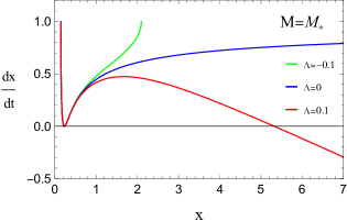
Figure 1: For outgoing null geodesics, we have plotted the case of the black hole with mass $M_{*}$ and compared three different spacetimes. AdS spacetime is taken to have $\Lambda=-0.1$, while dS spacetime has $\Lambda=0.1$. It can be observed that the three spacetimes exhibit little difference near the Killing horizon, and only significant differences arise far from the horizon. The remaining parameters are taken as $\left\{\gamma=1,\Delta=0.01,G=1\right\}$.

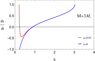
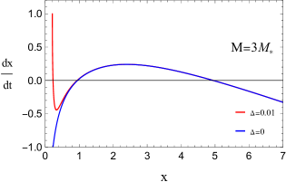
Figure 2: For outgoing null geodesics, we have separately plotted the cases of the AdS black holes (first figure) and the dS black holes (second figure) with the mass of $3M_{*}$. In both figures, the red curve represents the LQG-corrected metric, while the blue curve means the classical metric. For AdS black holes, we consider $\Lambda=-0.1$, whereas for dS black holes, $\Lambda=0.1$. All the remaining parameters are taken as $\left\{\gamma=1,G=1\right\}$.

From Fig 2, in the case of the LQG-corrected AdS black hole, the mass exceeds $M_{*}$, resulting in the presence of both inner and outer horizons. For LQG-corrected metric, the endpoints of the red curve correspond to the minimum and maximum values of $x$, where $dx/dt=1$, as can be easily verified by equations (52), (56), and (58). Conversely, the classical AdS black hole exhibits only one horizon, and $dx/dt$ diverges rapidly as $x\rightarrow 0$, indicating the presence of the spacetime singularity. In the case of dS black hole, the LQG correction also results in the existence of two Killing horizons, avoiding the singularity issue. Additionally, the cosmological horizon can be observed from the curves.

IV.2 Curvature scalars and surface gravity

Investigating the curvature of this effective metric can provide us with a deeper understanding of the geometric structure of this spacetime. Furthermore, it allows for a more straightforward comparison to be made with the scenario where the cosmological constant is not present. With the corrected metric 51, various curvature scalars can be straightforwardly calculated. The results are summarized as follows:

$$R=4\Lambda-\frac{4}{3}\gamma^{2}\Delta\Lambda^{2}-\frac{24(GM\gamma)^{2}\Delta}{x^{6}},$$ (59)

$$R_{\mu\nu}R^{\mu\nu}=\frac{4}{9}\Lambda^{2}\left(-3+\gamma^{2}\Delta\Lambda\right)^{2}+\frac{1440(GM\gamma)^{4}\Delta^{2}}{x^{12}}$$

$$+\frac{16(GM\gamma)^{2}\left(-3+\gamma^{2}\right)\Delta\Lambda}{x^{6}},$$ (60)

$$R_{\mu\nu\rho\sigma}R^{\mu\nu\rho\sigma} = \frac{8}{27}\Lambda^{2}\left(-3+\gamma^{2}\Delta\Lambda\right)^{2}$$ (61)

$$+ \frac{320(GM)^{3}\gamma^{2}\left(-3+2\gamma^{2}\Delta\Lambda\right)\Delta}{x^{9}}$$

$$+ \frac{32\left(GM\gamma\right)^{2}\left(-3+\gamma^{2}\Delta\Lambda\right)\Delta\Lambda}{x^{6}}$$

$$+ \frac{7488(GM\gamma)^{4}\Delta^{2}}{{x}^{12}}.$$

For physical reasons, the absolute value of curvature scalars should correspond to a maximum when $x$ approaches $x_{min}$ in vacuum. By substituting $x_{min}$ into various curvature scalars, we obtain the following results

$$\lim_{x\to x_{\min}}R=-\frac{6}{\gamma^{2}\Delta}+8\Lambda-2\gamma^{2}\Delta\Lambda^{2},$$ (62)

$$\lim_{x\to x_{\min}}R_{\mu\nu}R^{\mu\nu}$$

$$=\frac{2\left(-3+\gamma^{2}\Delta\Lambda\right)^{2}\left(5-4\gamma^{2}\Delta\Lambda+\gamma^{4}\Delta^{2}\Lambda^{2}\right)}{\gamma^{4}\Delta^{2}},$$ (63)

$$\lim_{x\to x_{\min}}R_{\mu\nu\rho\sigma}R^{\mu\nu\rho\sigma}$$

$$=\frac{4\left(-3+\gamma^{2}\Delta\Lambda\right)^{2}\left(10-6\gamma^{2}\Delta\Lambda+\gamma^{4}\Delta^{2}\Lambda^{2}\right)}{\gamma^{4}\Delta^{2}}.$$ (64)

These are also constants independent of the black hole mass. Unsurprisingly, when the terms containing the cosmological constant are discarded, these curvature scalars align with those in [27] [28].

In addition, exploring the trapped surface can further verify the results of the effective metric we have obtained. Considering the null geodesic congruence, due to the spherical symmetry, on a 2-dimensional sphere $S$, the radial coordinate $x$ and the time coordinate $t$ are constant. Therefore, there are two independent null tangent vectors orthogonal to $S$, referred to as outgoing null geodesics and ingoing null geodesics. These two geodesics correspond to the outgoing expansion parameter $\theta_{+}$ and ingoing expansion parameter $\theta_{-}$ respectively. By definition, the trapped surface corresponds to the region where both $\theta_{+}$ and $\theta_{-}$ are negative. Here, we define the tangent vectors of the outgoing null geodesics and the ingoing null geodesics to be the same as [27], denoted by

$$l^{\mu}=\left(\frac{\partial}{\partial t}\right)^{\mu}+(1-N^{x})\left(\frac{\partial}{\partial x}\right)^{\mu},$$ (65)

and

$$k^{\mu}=\left(\frac{\partial}{\partial t}\right)^{\mu}+(-1-N^{x})\left(\frac{\partial}{\partial x}\right)^{\mu}.$$ (66)

Normalize these two vector fields such that $l^{\mu}k_{\mu}=-2$ and the hypersurface metric for $S$ is

$$h_{\mu\nu}=g_{\mu\nu}+\frac{1}{2}\left(l_{\mu}k\nu+k_{\mu}l_{\nu}\right).$$ (67)

Based on the definition of the expansions $\theta_{+}$ and $\theta_{-}$, the simple expression can be obtained through straightforward calculations and the results are

$$\theta_{+} = h^{\mu\nu}\nabla_{\mu}l_{\nu}=\frac{2}{x}\left(1-N^{x}\right),$$ (68)

$$\theta_{-} = h^{\mu\nu}\nabla_{\mu}k_{\nu}=-\frac{2}{x}\left(1+N^{x}\right).$$ (69)

Here, $\theta_{-}$ remains negative within the range of $x$, so considering $\theta_{+}$ alone is sufficient. The main results are displayed in Figure 4 and 4. Besides, the trapped surface tends to increase with the increase of mass. From the expression of the expansion (68) and the null geodesic (58), it can be observed that they differ only by a factor of $2/x$. Therefore, it is conceivable that the zero points of the null geodesics align with the outgoing expansion and the physical interpretation is consistent with the null geodesics.

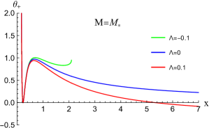
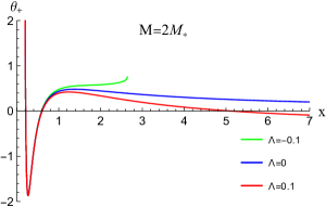
Figure 3: The expansions of the outgoing null geodesics are compared for different cosmological constants. In this case, the mass is chosen as $M_{*}$, indicating that when $\Lambda=0$ , there is only one event horizon. More detailed calculations reveal when $\Lambda=-0.1$, there is no event horizon and the curve’s endpoint cannot extend indefinitely but reaches a certain point. This also implies the maximum value that $x$ can take. When $\Lambda=0.1$, there are two close inner and outer horizons, and a cosmological horizon can be clearly observed at the end of the curve. These properties are analogous to those of the outgoing null geodesics. The remaining parameters are taken as $\left\{\gamma=1,\Delta=0.01,G=1\right\}$.

Figure 4: Comparison of the null expansion $\theta_{+}$ for the LQG-corrected metric with different values of the cosmological constant. The mass is $2M_{*}$, compared to the case with mass $M_{*}$, the most notable difference is that regardless of the value of the cosmological constant, the black hole exhibits both inner and outer event horizons. The influence of the cosmological constant is only evident at the endpoint of the curve. The remaining parameters are taken as $\left\{\gamma=1,\Delta=0.01,G=1\right\}$.

When a black hole possesses an outer horizon, it becomes straightforward to calculate the surface gravity by employing

$$\kappa=\left.\frac{1}{2}\frac{\partial F(x)}{\partial x}\right|_{x=x_{out}}.$$ (70)

where $x_{out}$ represents the position of the outer horizon. Due to the complexity of the expression of $F(x)$, it is not practical to calculate the analytical solution of the surface gravity directly. Moreover, if we adopt a first-order approximation for $\Delta$, the distinctions between the three types of spacetime will not be apparent and the result of the expression will be the same. Therefore, we adopt a numerical approach to solve the problem. The detailed results are shown in Figure 5.

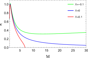
Figure 5: By taking the mass of the black hole as the independent variable, we compared the surface gravity under different values of the cosmological constant. The mass is measured in units of $M_{*}$. The minimum value of the mass is set at $M_{*}$ because when the mass is less than $M_{*}$, there is no horizon, and any discussion concerning surface gravity becomes meaningless. The remaining parameters are taken as $\left\{\gamma=1,\Delta=0.01,G=1\right\}$.

The green curve corresponds to the AdS black hole, and the red curve represents the dS black hole. At smaller masses, due to the LQG correction, they behave almost identically and both exhibit a peak. However, as the mass increases, due to the distinct characteristics of the spacetime, the surface gravity of the dS black hole rapidly tends to zero and eventually reaches an upper mass limit, whereas the surface gravity of the AdS black hole first decreases and then slowly increases.

V Conclusions and discussions

The main result in this paper is obtained based on the Painlevé-Gullstrand coordinate system and utilizes the components of the Ashtekar-Barbero connection and density-triad to describe a 4-dimensional spherically symmetric spacetime with a cosmological constant. We first perform calculations in the classical scenario. Starting from the gravitational action, after symmetry reduction, we consider the constrained system to consist of Hamiltonian constraint (scalar constraint) and the diffeomorphism constraint (vector constraint) due to the constrained nature of the system. By exploiting the spherical symmetry, further simplification of the constraints can be achieved. The equations of motion can then be obtained.

Then we impose a gauge fixing on the area and select a particular Painlevé-Gullstrand coordinate system $(N=1)$ [27]. As a result, the number of dynamical variables is reduced from four to two, and the equations of motion are also reduced to two. By directly solving the equations, the classical Schwarzschild de-Sitter(anti-de Sitter) solutions are obtained as expected.

We then modified the variable $p$ of the connection by incorporating holonomy corrections and adjusted the Hamiltonian constraint, symplectic structure, and shift vector accordingly. Similarly, by solving the modified effective equations of motion, we obtained the LQG-corrected spherically symmetric metric with a cosmological constant.

Due to the LQG correction, the variable $x$ has a restricted range of values. For AdS and dS spacetimes, we calculated their common minimum value $x_{min}$ using timelike geodesics. The dS spacetime exhibits the expected cosmological horizon. The effect of the cosmological constant is only noticeable at distances far from the event horizon which is consistent with the expectations. We also investigated the curvature scalars $R,R_{\mu\nu}R^{\mu\nu},R_{\mu\nu\rho\sigma}R^{\mu\nu\rho\sigma}$ of the LQG-corrected metric, which are bounded at $x_{min}$ due to quantum gravity effects and are constants that only depend on $\Lambda$ and $\Delta$. Moreover, when setting $\Lambda=0$, all the curvature scalars can be recovered in the form presented in article [27].

It is worth mentioning that the computation of $x_{min}$ can also be directly obtained from $F(x)$. Since $F(x)=1-\left(N^{x}\right)^{2}$, it can be observed that $F(x)\leq 1$, and when $F(x)=1$, it represents the boundary of applicability for $F(x)$. And $x_{min}$ is one of the solutions to $F(x)=1$.

Furthermore, we plotted the figure of the outgoing expansion, which shares similar properties with the outgoing null geodesics due to their expressions differing only by a factor of $2/x$. In addition, we also present the plot of surface gravity, it is observed that in the dS spacetime, as the black hole mass increases, $\kappa$ rapidly decreases and approaches zero, whereas in the AdS spacetime, $\kappa$ continues to slowly increase.

- [1] A. Ashtekar and J. Lewandowski, Background Independent Quantum Gravity: A Status Report, Class. Quantum Grav. 21, R53 (2004).
- [2] C. Rovelli, Quantum Gravity (Cambridge University Press, Cambridge, England, 2004).
- [3] T. Thiemann, Modern Canonical Quantum General Relativity (Cambridge University Press, Cambridge, United Kingdom, 2007).
- [4] M. Han, Y. Ma, and W. Huang, Fundamental structure of loop quantum gravity, Int. J. Mod. Phys. D 16, 1397 (2007).
- [5] C. Rovelli and L. Smolin, Discreteness of Area and Volume in Quantum Gravity, Nuclear Physics B 442, 593 (1995).
- [6] A. Ashtekar and J. Lewandowski, Quantum Theory of Geometry: I. Area Operators, Class. Quantum Grav. 14, A55 (1997).
- [7] A. Ashtekar and J. Lewandowski, Quantum Theory of Geometry II: Volume Operators, Adv. Theor. Math. Phys. 1, 388 (1997).
- [8] J. Yang and Y. Ma, New Volume and Inverse Volume Operators for Loop Quantum Gravity, Phys. Rev. D 94, 044003 (2016).
- [9] T. Thiemann, A Length Operator for Canonical Quantum Gravity, Journal of Mathematical Physics 39, 3372 (1998).
- [10] Y. Ma, C. Soo, and J. Yang, New Length Operator for Loop Quantum Gravity, Phys. Rev. D 81, 124026 (2010).
- [11] X. Zhang and Y. Ma, Extension of Loop Quantum Gravity to f (R) Theories, Phys. Rev. Lett. 106, 171301 (2011).
- [12] N. Bodendorfer, T. Thiemann, and A. Thurn, New Variables for Classical and Quantum Gravity in All Dimensions I. Hamiltonian Analysis, Class. Quantum Grav. 30, 045001 (2013).
- [13] X. Zhang, J. Yang, and Y. Ma, Canonical Loop Quantization of the Lowest-Order Projectable Horava Gravity, Phys. Rev. D 102, 124060 (2020).
- [14] H. Tan and Y. Ma, Semiclassical States in Homogeneous Loop Quantum Cosmology, Class. Quantum Grav. 23, 6793 (2006).
- [15] M. Bojowald, Absence of a Singularity in Loop Quantum Cosmology, Phys. Rev. Lett. 86, 5227 (2001).
- [16] L. Modesto, Disappearance of the Black Hole Singularity in Loop Quantum Gravity, Phys. Rev. D 70, 124009 (2004).
- [17] A. Ashtekar and M. Bojowald, Quantum Geometry and the Schwarzschild Singularity, Class. Quantum Grav. 23, 391 (2005).
- [18] A. Ashtekar, M. Bojowald, and J. Lewandowski, Mathematical Structure of Loop Quantum Cosmology, Advances in Theoretical and Mathematical Physics 7, 233 (2003).
- [19] M. Bojowald, Loop Quantum Cosmology, Living Rev. Relativ. 11, 4 (2008).
- [20] A. Ashtekar and P. Singh, Loop Quantum Cosmology: A Status Report, Class. Quantum Grav. 28, 213001 (2011).
- [21] C. G. Boehmer and K. Vandersloot, Loop Quantum Dynamics of the Schwarzschild Interior, Phys. Rev. D 76, 104030 (2007).
- [22] D.-W. Chiou, Phenomenological Loop Quantum Geometry of the Schwarzschild Black Hole, Phys. Rev. D 78, 064040 (2008).
- [23] A. Ashtekar, J. Olmedo, and P. Singh, Quantum Transfiguration of Kruskal Black Holes, Phys. Rev. Lett. 121, 241301 (2018).
- [24] C. Zhang and X. Zhang, Quantum geometry and effective dynamics of Janis-Newman-Winicour singularities, Phys. Rev. D 101, 086002 (2020),
- [25] J. Lewandowski, Y. Ma, J. Yang, and C. Zhang, Quantum Oppenheimer-Snyder and Swiss Cheese Models, Phys. Rev. Lett. 130, 101501 (2023).
- [26] X. Zhang, Loop Quantum Black Hole, Universe 9, 313 (2023).
- [27] J. G. Kelly, R. Santacruz, and E. Wilson-Ewing, Effective Loop Quantum Gravity Framework for Vacuum Spherically Symmetric Spacetimes, Phys. Rev. D 102, 106024 (2020).
- [28] R. Gambini, J. Olmedo, and J. Pullin, Spherically symmetric loop quantum gravity: Analysis of improved dynamics, Classical Quantum Gravity 37, 205012 (2020).