A Riemann-Hilbert approach to the two-component modified Camassa-Holm equation on the line

Abstract

In this paper, we develop a Riemann-Hilbert approach to the Cauchy problem for the two-component modified Camassa-Holm (2-mCH) equation based on its Lax pair. Further via a series of deformations to the Riemann-Hilbert problem associated with the Cauchy problem by using the $\bar{\partial}$-generalization of Deift-Zhou steepest descent method, we obtain the long-time asymptotic approximations of the solutions of the 2-mCH equation in four space-time regions. Our results also confirm the soliton resolution conjecture and asymptotically stability of the $N$-soliton solutions for the 2-mCH equation.
Keywords: two-component modified Camassa-Holm equation, Inverse Scattering Transform, Riemann-Hilbert problem, $\overline{\partial}$-steepest descent method, long-time asymptotics.
MSC 2020: 35Q51; 35Q15; 37K15; 35C20.

1 Introduction

In this paper, we develop the Riemann-Hilbert (RH) approach to the Cauchy problem of the two-component modified Camassa-Holm (2-mCH) equation

$$\tilde{m}_{t}+[(u-u_{x})(v+v_{x})\tilde{m}]_{x}=0,\quad t>0,\ x\in\mathbb{R},$$ (1.1)

$$\tilde{n}_{t}+[(u-u_{x})(v+v_{x})\tilde{n}]_{x}=0,\ \ \tilde{m}:=u-u_{xx},\quad\tilde{n}:=v-v_{xx},$$ (1.2)

$$u(x,0)=u_{0}(x),\ \ v(x,0)=v_{0}(x),$$ (1.3)

where $u_{0},v_{0}\in H^{4,2}(\mathbb{R})$ with the nonzero boundary conditions

$$u_{0}(x)\to 1,\quad v_{0}(x)\to 1,\ \ x\to\infty.$$ (1.4)

The Camassa-Holm (CH) equation is one of the most famous integrable equations, which was first presented by Camassa and Holm [1]. Later the CH equation was generalized into a modified Camassa-Holm (mCH) equation in the works of Fokas [2] and Fuchssteiner [3] as well as Olver and Rosenau [4]. Much works on these two equations can be found in [8, 9, 10, 11, 12, 13, 14, 15, 16, 17, 18, 19, 20, 21, 22, 23, 27, 30, 24, 25, 26, 28, 29, 31, 32, 33].

As a two-component integrable extension of the mCH equation [5], the 2-mCH equation (1.1)-(1.2) also draws some attentions in recent years. For example, Tian and Liu obtained the 2-mCH equation and found its bi-Hamiltonian structure by applying tri-Hamiltonian duality into the bi-Hamiltonian representation of the Wadati-Konno-Ichikawa equation [6]; Chang et al presented an explicit construction of peakon solutions for the 2-mCH equation (1.1)-(1.2), and discussed the global existence and the large time asymptotics of the peakon solutions [7]. To the best of our knowledge, the inverse scattering transform or RH method have not yet been applied to the 2-mCH equation (1.1)-(1.2). The purpose of our paper is to present the RH approach to the Cauchy problem of the 2-mCH equation and further analyze the long time asymptotic behavior.

We define two new functions $\tilde{u},\tilde{v}$ by

$$u(x,t)=\tilde{u}(x-t,t)+1,$$ (1.5)

$$v(x,t)=\tilde{v}(x-t,t)+1,$$ (1.6)

and define a transformation

$$p(x,t):=\tilde{u}-\tilde{u}_{x}+1,\quad q(x,t):=\tilde{v}+\tilde{v}_{x}+1,$$ (1.7)

then the Cauchy problem (1.1)-(1.4) is changed into the following Cauchy problem that we consider in our paper

$$m_{t}+(wm)_{x}=0,\ \ n_{t}+(wn)_{x}=0,\ \ t>0,x\in\mathbb{R}$$ (1.8)

$$m=p+p_{x},\ \ n=q-q_{x},\ \ w=pq-1,$$ (1.9)

$$p(x,0)=p_{0}(x),\ q(x,0)=q_{0}(x),$$ (1.10)

where $p_{0},q_{0}\in H^{4,2}(\mathbb{R})$ and as

$$\ p_{0}(x)\to 1,\ q_{0}(x)\to 1,\quad x\to\infty.$$ (1.11)

Our main results are stated as follows.

Theorem 1.

Let $p(x,t)$ and $q(x,t)$ be the solutions for the initial-value problem (1.8)-(1.10) with generic data $p_{0},q_{0}\in H^{4,2}(\mathbb{R})$ and scatting data ${\mathcal{D}}_{\Lambda}=\left\{r(z),\left\{\zeta_{n},C_{n}T^{2}(\zeta_{n})\right\}^{4N_{1}+2N_{2}}_{n=1}\right\}$. And $p^{r}_{\Lambda}(x,t;\tilde{\mathcal{D}})$ and $q^{r}_{\Lambda}(x,t;\tilde{\mathcal{D}})$ denote the $\mathcal{N}(\Lambda)$-soliton solution corresponding to reflectionless scattering data $\tilde{\mathcal{D}}_{\Lambda}=\left\{0,\left\{\zeta_{n},C_{n}\right\}_{n\in\Lambda}\right\}$. Then there exist a large constant $T_{1}=T_{1}(\xi),\ \xi=\frac{y}{t}$, such that for all $T_{1}<t\to\infty$,

1. For $\xi\in(-\infty,-1/4)\cup(2,+\infty)$, we have asymptotic expansion

$$(\log p)_{x}=p^{r}(x,t;{\mathcal{D}}_{\Lambda})+\mathcal{O}(t^{-1+2\rho}),$$

$$(\log q)_{x}=q^{r}(x,t;{\mathcal{D}}_{\Lambda})+\mathcal{O}(t^{-1+2\rho}),$$

with

$$x(y,t)=y+2\ln T(i)+c_{+}^{r}(x,t;\tilde{\mathcal{D}}_{\Lambda})+\mathcal{O}(t^{-1+2\rho}).$$

2. For $\xi\in(-1/4,0)\cup(0,2)$, we have asymptotic expansion

$$(\log p)_{x}=p^{r}(x,t;{\mathcal{D}}_{\Lambda})+f_{11}t^{-1/2}+\mathcal{O}(t^{-3/4}),$$

$$(\log q)_{x}=q^{r}(x,t;{\mathcal{D}}_{\Lambda})+f_{21}t^{-1/2}+\mathcal{O}(t^{-3/4}),$$

with

$$x(y,t)=y-2\ln\left(T(i)\right)+c_{+}^{r}(x,t;\tilde{\mathcal{D}}_{\Lambda})+f_{12}t^{-1/2}+\mathcal{O}(t^{-3/4}).$$

Our results also confirm the soliton resolution conjecture and asymptotically stability of the $N$-soliton solutions for the 2-mCH equation.

Our paper is organized as follows. In section 2, we develop a Riemann-Hilbert(RH) approach to the 2-mCH equation by the method of Inverse Scattering Transform(IST). Then in section 3 and 4, based on the RH representation, we apply the $\bar{\partial}$-steepest descent method to study the long-time asymptotic behavior for the solution of the 2-mCH equation in two cases.

2 Inverse scattering transform and the RH problem

In this section, we study the inverse scattering transform and the RH problem associated with the Cauchy problem (1.8)-(1.10).

2.1 Spectral analysis on Lax pair

The 2-mCH equation (1.8)-(1.9) admits the conservation law

$$-(\sqrt{mn})_{t}=(w\sqrt{mn})_{x},$$ (2.1)

and the following Lax pair:

$$\Psi_{x}=U\Psi,\quad\Psi_{t}=V\Psi,$$ (2.2)

where

$$U=\frac{1}{2}\left(\begin{array}[]{cc}-1&\lambda m\\ -\lambda n&1\end{array}\right),$$ (2.5)

$$V=\left(\begin{array}[]{cc}\lambda^{-2}+\frac{w}{2}&-\lambda^{-1}(u-u_{x}+c)-\frac{\lambda}{2}wm\\ \lambda^{-1}(v+v_{x}+1)+\frac{\lambda}{2}wn&-\lambda^{-2}-\frac{w}{2}\end{array}\right),\qquad$$ (2.8)

By the boundary condition (1.11), we find that as $x\to\infty$,

$$m(x,0)\to c,\quad n(x,0)\to 1,\quad w(x,0)\to 0.$$ (2.9)

To keep the symmetry and zero trace of the matrix $U$ in Lax pair (2.2), we first take the transformation

$$\hat{\Psi}(x,t,\lambda)=A(x,t)\hat{\Psi}(x,t,\lambda)$$ (2.10)

with

$$A(x,t)=(mn)^{-\frac{1}{4}}\left(\begin{array}[]{cc}\sqrt{m}&0\\ 0&\sqrt{n}\end{array}\right).$$ (2.11)

Then the Lax pair (2.2) changes into

$$\hat{\Psi}_{x}=\hat{U}\hat{\Psi},\quad\hat{\Psi}_{t}=\hat{V}\hat{\Psi},$$ (2.12)

where

$$\hat{U}=\frac{1}{2}\left(\begin{array}[]{cc}-1&\lambda\sqrt{mn}\\ -\lambda\sqrt{mn}&1\end{array}\right)+\left(\begin{array}[]{cc}\frac{mn_{x}-m_{x}n}{4mn}&0\\ 0&-\frac{mn_{x}-m_{x}n}{4mn}\end{array}\right),$$ (2.17)

$$\hat{V}=\left(\begin{array}[]{cc}\lambda^{-2}+\frac{w}{2}&-\sqrt{\frac{n}{m}}[\lambda^{-2}p+\frac{\lambda}{2}wm]\\ \sqrt{\frac{m}{n}}[\lambda^{-1}q+\frac{\lambda}{2}wn]&-\lambda^{-2}-\frac{w}{2}\end{array}\right)+\left(\begin{array}[]{cc}\frac{mn_{t}-m_{t}n}{4mn}&0\\ 0&-\frac{mn_{t}-m_{t}n}{4mn}\end{array}\right).\qquad\quad$$ (2.22)

Notice that the coefficients of the Lax pair (2.12) have singularities at $\lambda=0$ and $\lambda=\infty$. To have a good control on the asymptotic behavior of eigenfunctions, we use two different transformations to get new forms of (2.12), which are appropriat at $k=0$ and $k=\infty$ respectively.

Case I: $\lambda=\infty$

Make the transformation

$$\hat{\Phi}(x,t,\lambda)=D(\lambda)\hat{\Psi}(x,t,\lambda)$$

with

$$D(\lambda)=\left(\begin{array}[]{cc}1&-\frac{\lambda}{1+\sqrt{1-\lambda^{2}}}\\ -\frac{\lambda}{1+\sqrt{1-\lambda^{2}}}&1\end{array}\right),\ \ \lambda=\frac{1}{2}(k+k^{-1}),$$ (2.23)

then $\hat{\Phi}$ satisfies the following Lax pair

$$\hat{\Phi}_{x}+\frac{i(k^{2}-1)}{4k}\sqrt{mn}\sigma_{3}\hat{\Phi}=\tilde{U}\hat{\Phi},$$ (2.24)

$$\hat{\Phi}_{t}-\left[\frac{i(k^{2}-1)}{4k}w\sqrt{mn}+\frac{2ik(k^{2}-1)}{(k^{2}+1)^{2}}\right]\sigma_{3}\hat{\Phi}=\tilde{V}\hat{\Phi},$$ (2.25)

where

$$\tilde{U}(k)=-\frac{ik}{k^{2}-1}\left(\sqrt{mn}-1+\frac{mn_{x}-m_{x}n}{2mn}\right)\sigma_{3}-\frac{i(k^{2}+1)}{2(k^{2}-1)}\left(\sqrt{mn}-1+\frac{mn_{x}-m_{x}n}{2mn}\right)\left(\begin{array}[]{cc}0&1\\ -1&0\end{array}\right),$$ (2.28)

$$\tilde{V}(k)=\frac{ik}{k^{2}-1}\left(w(\sqrt{mn}-1)-\frac{mn_{t}-m_{t}n}{2mn}\right)\sigma_{3}+\frac{ik}{k^{2}-1}\left(\sqrt{\frac{n}{m}}p+\sqrt{\frac{m}{n}}q-2\right)\sigma_{3}$$

$$\qquad\quad\ +\frac{i(k^{2}+1)}{2(k^{2}-1)}\left(w(\sqrt{mn}-1)-\frac{mn_{t}-m_{t}n}{2mn}\right)\left(\begin{array}[]{cc}0&1\\ -1&0\end{array}\right)-\frac{4ik^{2}}{k^{4}-1}\left(\begin{array}[]{cc}0&1\\ -1&0\end{array}\right)$$ (2.33)

$$\qquad\quad\ +\left(\begin{array}[]{cc}0&-\frac{k(k-i)p}{(k^{2}-1)(k+i)}\sqrt{\frac{n}{m}}+\frac{k(k+i)q}{(k^{2}-1)(k-i)}\sqrt{\frac{m}{n}}\\ \frac{k(k-i)q}{(k^{2}-1)(k+i)}\sqrt{\frac{m}{n}}-\frac{k(k+i)p}{(k^{2}-1)(k-i)}\sqrt{\frac{n}{m}}&0\end{array}\right).$$ (2.36)

By the conservation law, we define a new function

$$\tilde{p}(x,t,k)=-\frac{i(k^{2}-1)}{4k}\int_{x}^{\infty}(\sqrt{mn}-1)\mathrm{d}s+\frac{i(k^{2}-1)}{4k}x-\frac{2ik(k^{2}-1)}{(k^{2}+1)^{2}}t.$$ (2.37)

then

$$\tilde{p}_{x}=\frac{i(k^{2}-1)}{4k}\sqrt{mn},\quad\tilde{p}_{t}=-\frac{i(k^{2}-1)}{4k}w\sqrt{mn}-\frac{2ik(k^{2}-1)}{(k^{2}+1)^{2}},$$ (2.38)

and $\tilde{p}_{xt}=\tilde{p}_{tx}$.

As $x\to\infty$, $\tilde{U},\tilde{V}\to 0$, thus $\hat{\Phi}\sim e^{-\tilde{p}(x,t,k)\sigma_{3}}$. Take the transformation

$$\Phi(x,t,k)=\hat{\Phi}(x,t,k)e^{\tilde{p}(x,t,k)\sigma_{3}},$$ (2.39)

then $\Phi(x,t,k)\to I,\quad x\to\infty$ and $\Phi$ satisfies the new Lax pair

$$\Phi_{x}+\tilde{p}_{x}[\sigma_{3},\Phi]=\tilde{U}\Phi,\quad\Phi_{t}+\tilde{p}_{t}[\sigma_{3},\Phi]=\tilde{V}\Phi,$$ (2.40)

where Jost solutions $\Phi_{\pm}$ admit the following Volterra integral equations

$$\Phi_{\pm}=I+\int_{\pm\infty}^{x}e^{-\frac{i(k^{2}-1)}{4k}\int_{y}^{x}\sqrt{mn}\mathrm{d}s\hat{\sigma_{3}}}\left[\tilde{U}(y,t,k)\Phi_{\pm}(y,t,k)\right]\mathrm{d}y.$$ (2.41)

Denote $\Phi_{\pm}=\left(\Phi_{\pm}^{(1)},\Phi_{\pm}^{(2)}\right),$ where $\Phi_{\pm}^{(1)}$ and $\Phi_{\pm}^{(2)}$ are the first and second columns of $\Phi_{\pm}$, respectively. By the equations (2.41), $\Phi_{\pm}$ have the following properties

Proposition 1.

Suppose the initial data $u_{0},v_{0}\in H^{4,2}(\mathbb{R})$, then we have

• $\Phi_{+}^{(1)}(k),\ \Phi_{-}^{(2)}(k)$ are analytical in the lower-half complex plane $\mathbb{C}^{-}:=\{k:\mathrm{Im}k<0\}$; $\Phi_{+}^{(2)}(k),\ \Phi_{-}^{(1)}(k)$ are analytical in the upper-half complex plane $\mathbb{C}^{+}:=\{k:\mathrm{Im}k>0\}$.

• The Jost functions $\Phi_{\pm}(k)$ admit the following symmetries

  $$\Phi(k)=\overline{\Phi(\bar{k}^{-1})}=\sigma_{1}\overline{\Phi(\bar{k})}\sigma_{1}=\sigma_{2}\Phi(-k)\sigma_{2}.\\$$ (2.42)

• Asymptotic behaviors: As $k\to\pm\infty$,

  $$\left(\Phi_{-}^{(1)}(k),\Phi_{+}^{(2)}(k)\right)\to I,\quad\left(\Phi_{+}^{(1)}(k),\Phi_{-}^{(2)}(k)\right)\to I;$$ (2.43)

  As $k\to\pm 1$,

  $$\Phi(x,t,k)=\pm\frac{i}{k\mp 1}\alpha_{\pm}(x,t)\left(\begin{array}[]{cc}\pm 1&1\\ -1&\mp 1\end{array}\right)+\mathcal{O}(1),\quad k\to\pm 1,$$ (2.44)

  where $\alpha_{\pm}(x,t)$ are real-valued functions.

As two solutions of the Lax pair (2.24)-(2.25), $\hat{\Phi}_{\pm}(k)$ satisfy a linear relation

$$\hat{\Phi}_{+}(k)=\hat{\Phi}_{-}(k)S(k),$$ (2.45)

together with (2.39), we get

$$\Phi_{+}(k)=\Phi_{-}(k)e^{-\tilde{p}(x,t,k)\hat{\sigma}_{3}}S(k),$$ (2.46)

where $S(k)$ is the scattering matrix defined as

$$S(k)=\left(\begin{array}[]{cc}s_{11}(k)&s_{12}(k)\\ s_{21}(k)&s_{22}(k)\end{array}\right).$$ (2.47)

By the symmetries of $\Phi(k)$, we find

$$S(k)=\sigma_{1}\overline{S(\bar{k})}\sigma_{1}=\sigma_{2}S(-k)\sigma_{2},$$ (2.48)

thus we can rewrite $S(k)$ as

$$S(k)=\left(\begin{array}[]{cc}\overline{a(\bar{k})}&b(k)\\ \overline{b(\bar{k})}&a(k)\end{array}\right)=\left(\begin{array}[]{cc}a(-k)&b(k)\\ -b(-k)&a(k)\end{array}\right).$$ (2.49)

From (2.46), $a(k),b(k)$ can be expressed as

$$a=\left|\Phi_{-}^{(1)}\ \Phi_{+}^{(2)}\right|,\quad b=e^{2p}\left|\Phi_{-}^{(2)}\ \Phi_{+}^{(2)}\right|,$$ (2.50)

so by the analyticity of $\Phi_{\pm}(k)$ in Proposition 1, we find $a(k)$ is analytic in $\mathbb{C}^{+}$.

Besides, the Jost solutions $\Phi_{\pm}(k)$ admit the asymptotics

$$\Phi_{\pm}(k)=I+\mathcal{O}(k^{-1}),\quad k\to\infty.$$ (2.51)

Combining (2.44), (2.50) with (2.51), we deduce the asymptotics of $a(k)$

$$a(k)=1+\mathcal{O}(k^{-1}),\quad k\to\infty;\qquad a(k)=\frac{\beta_{\pm}(x,t)}{k\pm 1}+\mathcal{O}(1),\quad k\to\pm 1,$$ (2.52)

where $\beta_{\pm}(x,t)$ are unknown functions.

Suppose that $a(k)$ has $N_{1}$ simple zeros $\mu_{1},\cdots,\mu_{N_{1}}$ on $\{k\in\mathbb{C}^{+}:0<\arg k<\frac{\pi}{2},|k|>1\}$, and $N_{2}$ simple zeros $\nu_{1},\cdots,\nu_{N_{2}}$ on the circle $\{k=e^{i\psi}:0<\psi<\frac{\pi}{2}\}$. The symmetries of $S(k)$ imply that

$$a(\mu_{n})=0\Leftrightarrow a(-\mu_{n}^{-1})=0\leftrightarrow a(\bar{\mu}_{n}^{-1})=0\leftrightarrow a(-\bar{\mu}_{n})=0,\quad n=1,\cdots,N_{1},$$ (2.53)

and on the circle

$$a(\nu_{m})=0\leftrightarrow a(-\bar{\nu}_{m})=0,\quad m=1,\cdots,N_{2}.$$ (2.54)

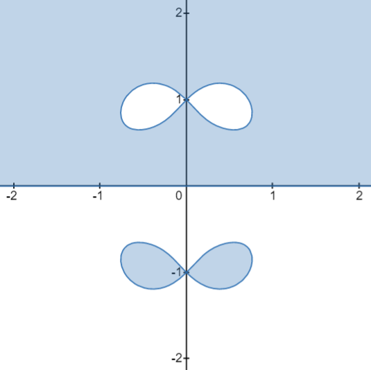
Now the zeros of $a(k)$ can be indicated as $\zeta_{n}=\mu_{n},\zeta_{n+N_{1}}=-\mu_{n}^{-1},\zeta_{n+N_{2}}=-\bar{\mu}_{n}$ and $\zeta_{n+3N_{1}}=\bar{\mu}_{n}^{-1}$ for $n=1,\cdots,N_{1}$; $\zeta_{m+4N_{1}}=\nu_{m},\zeta_{m+4N_{1}+N_{2}}=-\bar{\nu}_{m}$ for $m=1,\cdots,N_{2}$. Then $\bar{\zeta}_{n}$ is a simple zero of $\overline{a(\bar{k})}$. The discrete spectrum is $\mathbb{Z}:=\{\zeta_{n},\bar{\zeta}_{n}\}_{1}^{4N_{1}+2N_{2}}$, as shown in Figure 1.

Figure 1: The distribution of zeros of $a(k)$

Define the reflection coefficient as

$$r(k)=\frac{\overline{b(k)}}{a(k)},$$ (2.55)

then by the symmetry of $S(k)$, $r(k)$ is proved to admit the following symmetry:

$$r(k)=-\overline{r(-\bar{k})}=\overline{r(\bar{k}^{-1})}=-r(-r^{-1}).$$ (2.56)

Considering that as $k\to 0$, $a(k)\to 1$ and $b(k)\to 0$, we have $r(0)=0$.

Case II: $\lambda=0$

We rewrite the Lax pair (2.24)-(2.25) as

$$\hat{\Phi}_{x}+\left(\frac{i(k^{2}-1)}{4k}-\frac{ik}{k^{2}-1}\frac{mn_{x}-m_{x}n}{2mn}\right)\sigma_{3}\hat{\Phi}=\tilde{U}^{0}\hat{\Phi},$$ (2.57)

$$\hat{\Phi}_{t}-\frac{2ik(k^{2}-1)}{(k^{2}+1)^{2}}\sigma_{3}\hat{\Phi}=\tilde{V}^{0}\hat{\Phi},$$ (2.58)

where

$$\tilde{U}^{0}=-\frac{(k^{2}+1)^{2}}{4k(k^{2}-1)}(\sqrt{mn}-1)\sigma_{3}-\frac{i(k^{2}+1)}{2(k^{2}-1)}\left(\sqrt{mn}-1+\frac{mn_{x}-m_{x}n}{2mn}\right)\left(\begin{array}[]{cc}0&1\\ -1&0\end{array}\right),$$ (2.61)

$$\tilde{V}^{0}=\frac{ik}{k^{2}-1}\left(w(\sqrt{mn}-1)-\frac{mn_{t}-m_{t}n}{2mn}\right)\sigma_{3}+\frac{ik}{k^{2}-1}\left(\sqrt{\frac{n}{m}}p+\sqrt{\frac{m}{n}}q-2\right)\sigma_{3}+\frac{i(k^{2}-1)w}{4k}\sqrt{mn}\sigma_{3}$$

$$\qquad\quad\ +\frac{i(k^{2}+1)}{2(k^{2}-1)}\left(w(\sqrt{mn}-1)-\frac{mn_{t}-m_{t}n}{2mn}\right)\left(\begin{array}[]{cc}0&1\\ -1&0\end{array}\right)-\frac{4ik^{2}}{k^{4}-1}\left(\begin{array}[]{cc}0&1\\ -1&0\end{array}\right)$$ (2.66)

$$\qquad\quad\ +\left(\begin{array}[]{cc}0&-\frac{k(k-i)p}{(k^{2}-1)(k+i)}\sqrt{\frac{n}{m}}+\frac{k(k+i)q}{(k^{2}-1)(k-i)}\sqrt{\frac{m}{n}}\\ \frac{k(k-i)q}{(k^{2}-1)(k+i)}\sqrt{\frac{m}{n}}-\frac{k(k+i)p}{(k^{2}-1)(k-i)}\sqrt{\frac{n}{m}}&0\end{array}\right).$$ (2.69)

Take the transformation

$$\Phi^{0}(x,t,k)=\hat{\Phi}(x,t,k)e^{\left(\frac{ik}{2(k^{2}-1)}\ln\frac{n}{m}+\frac{i(k^{2}-1)}{4k}x-\frac{2ick(k^{2}-1)}{(k^{2}+1)^{2}}x\right)\sigma_{3}},$$ (2.70)

then as $x\to\infty$, $\Phi^{0}(x,t,k)\to I$, and $\Phi_{0}(k)$ admits the following Lax pair

$$\Phi^{0}_{x}+\left(\frac{i(k^{2}-1)}{4k}-\frac{ik}{k^{2}-1}\frac{mn_{x}-m_{x}n}{2mn}\right)[\sigma_{3},\Phi^{0}]=\tilde{U}^{0}\Phi^{0},$$ (2.71)

$$\Phi^{0}_{t}-\frac{2ik(k^{2}-1)}{(k^{2}+1)^{2}}[\sigma_{3},\Phi^{0}]=\tilde{V}^{0}\Phi^{0}.$$ (2.72)

The matrix function $\Phi^{0}(k)$ has the following asymptotic behavior as $k\to i$:

$$\Phi^{0}(x,t,k)=I+\left(\begin{array}[]{cc}f_{1}(t)&\frac{1}{2}\sqrt{\frac{m}{n}}q\\ \frac{1}{2}\sqrt{\frac{n}{m}}p&f_{2}(t)\end{array}\right)(k-i)+\mathcal{O}((k-i)^{2}),$$ (2.73)

where $f_{1}(t),f_{2}(t)$ are unknown functions only related to $t$.

Since $\Phi(k)$ and $\Phi^{0}(k)$ are solutions of two different Lax pair, which are all derived from the same Lax pair (2.24)-(2.25), they admit the linear relations as follows:

$$\Phi(k)=\Phi^{0}(k)e^{\left(\frac{i(k^{2}-1)}{4k}\int^{x}_{\pm\infty}(\sqrt{mn}-1)\mathrm{d}s-\frac{ik}{2(k^{2}-1)}\ln\frac{cn}{m}\right)\sigma_{3}}.$$ (2.74)

Therefore, together (2.73) with (2.74), the asymptotic behavior of $\Phi(k)$ at $k=i$ can be deduced.

2.2 Set up of a RH problem

We introduce a new scale

$$y:=\int_{x}^{+\infty}(\sqrt{mn}-1)\mathrm{d}s,$$ (2.75)

and write (2.37) in the form

$$\tilde{p}(x,t,k)=it\theta(k,\xi),$$ (2.76)

where

$$\theta(k,\xi)=\frac{k^{2}-1}{4\sqrt{c}k}\xi-\frac{2ck(k^{2}-1)}{(k^{2}+1)^{2}},\ \ \xi=\frac{y}{t}.$$ (2.77)

Define a matrix function

$$M(k):=M(y,t,k)=\left\{\begin{array}[]{lr}\left(\frac{\Phi_{-}^{(1)}}{a\left(k\right)}\quad\Phi_{+}^{(2)}\right),\quad\mathrm{Im}k>0,\\ \left(\Phi_{+}^{(1)}\quad\frac{\Phi_{-}^{(2)}}{\overline{a(\bar{k})}}\right),\quad\mathrm{Im}k<0,\end{array}\right.$$ (2.78)

which solves the following RH problem

RHP 1.

Find a $2\times 2$ matrix-valued function $M(k)$ satisfying

• Analyticity: $M(k)$ is meromorphic in $\mathbb{C}\setminus\mathbb{R};$

• Symmetry: $M(k)=\sigma_{1}\overline{M(\bar{k})}\sigma_{1}=\sigma_{2}M(-k)\sigma_{2}=\overline{M(\bar{k}^{-1})};$

• Jump condition: $M(k)$ has continuous boundary values $M_{\pm}(k)$ on $\mathbb{R}$ and

  $$M_{+}(k)=M_{-}(k)V(k),\quad k\in\mathbb{R},$$ (2.79)

  where

  $$V(k)=e^{-it\theta(k)\hat{\sigma}_{3}}V_{0}(k),$$ (2.80)

  and

  $$V_{0}(k)=\left(\begin{array}[]{cc}1-|r(k)|^{2}&\bar{r}(k)\\ -r(k)&1\end{array}\right);$$ (2.81)

• Asymptotic behaviors:

  $$M(k)=I+\mathcal{O}(k^{-1}),\quad k\to\infty;$$ (2.82)

  $$M(k)=\frac{i}{k-1}\alpha_{+}\left(\begin{array}[]{cc}0&1\\ 0&-1\end{array}\right)+\mathcal{O}(1),\quad k\to 1,\ \mathrm{Im}k>0;$$ (2.85)

  $$M(k)=\frac{i}{k-1}\alpha_{+}\left(\begin{array}[]{cc}1&0\\ -1&0\end{array}\right)+\mathcal{O}(1),\quad k\to 1,\ \mathrm{Im}k<0;$$ (2.88)

  $$M(k)=\frac{i}{k+1}\alpha_{-}\left(\begin{array}[]{cc}0&0\\ -1&-1\end{array}\right)+\mathcal{O}(1),\quad k\to 1,\ \mathrm{Im}k>0;$$ (2.91)

  $$M(k)=\frac{i}{k+1}\alpha_{-}\left(\begin{array}[]{cc}1&1\\ 0&0\end{array}\right)+\mathcal{O}(1),\quad k\to 1,\ \mathrm{Im}k>0;$$ (2.94)

  $$M(k)=e^{\tau_{+}\sigma_{3}}+e^{\tau_{+}\sigma_{3}}\left(\begin{array}[]{cc}f_{1}(t)&\frac{1}{2\sqrt{c}}\sqrt{\frac{m}{n}}q\\ \frac{1}{2\sqrt{c}}\sqrt{\frac{n}{m}}p&f_{2}(t)\end{array}\right)(k-i)+\mathcal{O}((k-i)^{2}),\quad k\to i,$$ (2.97)

  where

  $$\tau_{+}=\frac{1}{2\sqrt{c}}\int_{-\infty}^{+\infty}(\sqrt{mn}-1)\mathrm{d}s-\frac{1}{4}\ln\frac{cn}{m};$$ (2.98)

• Residue condition: $M(k)$ has simple poles at each $\zeta_{n}\in\mathcal{Z}$ with

  $$\operatorname*{Res}_{k=\zeta_{n}}M(k)=\lim_{k\to\zeta_{n}}M\left(\begin{array}[]{cc}0&0\\ c_{n}e^{2it\theta}&0\end{array}\right),$$ (2.101)

  $$\operatorname*{Res}_{k=\bar{\zeta}_{n}}M(k)=\lim_{k\to\overline{\mu}_{n}}M\left(\begin{array}[]{cc}0&\bar{c}_{n}e^{-2it\theta}\\ 0&0\end{array}\right),$$ (2.104)

  where $c_{n}=-\frac{\overline{b(\bar{\zeta_{n}})}}{a^{\prime}(\zeta_{n})},n=1,\cdots,4N_{1}+2N_{2}.$

Considering the asymptotics of $M(k)$ at $k=i$, we deduce the reconstruction formula for the solutions of the 2-mCH equation (1.8)-(1.9) as follows

$$\begin{array}[]{lr}\partial_{x}(\ln p)=-\partial_{x}(\ln G_{3})G_{1}^{-1}-1,\\ \partial_{x}(\ln q)=1-\partial_{x}(\ln G_{3})G_{2}^{-1},\end{array}$$ (2.105)

where

$$G_{1}=\lim_{k\to i}\frac{M_{21}(k)M_{22}(k)}{M_{11}(k)M_{12}(k)}-1,$$ (2.106)

$$G_{2}=\lim_{k\to i}\frac{M_{11}(k)M_{12}(k)}{M_{21}(k)M_{22}(k)}-1,$$ (2.107)

$$G_{3}=\lim_{k\to i}\frac{M_{12}(k)M_{21}(k)}{(k-i)^{2}},$$ (2.108)

and

$$x(y,t)=y+\ln\left(\lim_{k\to i}\frac{M_{11}(k)}{M_{22}(k)}\right)+\frac{1}{2}\ln c+\ln(q-q_{x})-\ln(p+p_{x}).$$ (2.109)

To remove the singularity of $M(k)$ at $k=\pm 1$, we introduce the following transformation

$$\left(I+\frac{\sigma_{1}}{k}\right)M(k)=\left(I+\frac{\sigma_{1}M^{J}(0)^{-1}}{k}\right)M^{J}(k).$$ (2.110)

Then matrix function $M^{J}(k)$ satisfies a new RH problem:

RHP 2.

Find a $2\times 2$ matrix-valued function $M^{J}(k)$ satisfying

• Analyticity: $M^{J}(k)$ is meromorphic in $\mathbb{C}\setminus\mathbb{R};$

• Symmetry: $M^{J}(k)=\sigma_{1}\overline{M^{J}(\bar{k})}\sigma_{1}=\sigma_{2}M^{J}(-k)\sigma_{2}=\sigma_{1}M^{J}(0)^{-1}M^{J}(k^{-1})\sigma_{1};$

• Jump condition: $M(k)$ has continuous boundary values $M^{J}_{\pm}(k)$ on $\mathbb{R}$ and

  $$M^{J}_{+}(k)=M^{J}_{-}(k)V(k),\quad k\in\mathbb{R};$$ (2.111)

• Residue condition: $M^{J}(k)$ has simple poles at each $\zeta_{n}\in\mathcal{Z}$ with

  $$\operatorname*{Res}_{k=\zeta_{n}}M^{J}(k)=\lim_{k\to\zeta_{n}}M^{J}(k)\left(\begin{array}[]{cc}0&0\\ c_{n}e^{2it\theta}&0\end{array}\right),$$ (2.114)

  $$\operatorname*{Res}_{k=\overline{\zeta}_{n}}M^{J}(k)=\lim_{k\to\overline{\zeta}_{n}}M^{J}(k)\left(\begin{array}[]{cc}0&\bar{c}_{n}e^{-2it\theta}\\ 0&0\end{array}\right),$$ (2.117)

  where $c_{n}=-\frac{\overline{b(\bar{\zeta_{n}})}}{a^{\prime}(\zeta_{n})},n=1,\cdots,4N_{1}+2N_{2}.$

Figure 2: The classification of $\text{sign Im}\theta$. In the blue regions, $\text{Im}\theta>0$, which implies that $|e^{2it\theta}|\to 0$ as $t\to\infty$. While in the white regions, $\text{Im}\theta<0$, which implies $|e^{-2it\theta}|\to 0$ as $t\to\infty$. The blue curves $\text{Im}\theta=0$ are critical lines between decay and growth regions.

To deal with the oscillatory terms $e^{\pm 2it\theta}$ in the jump matrix and residue conditions of RHP 1, we consider the real part of $2it\theta$:

$$\mathrm{Re}(2it\theta)=-2t\mathrm{Im}k\left[\frac{\xi}{4\sqrt{c}}(1+|k|^{-2})+2c\dfrac{|z|^{6}-2|z|^{4}-(3\text{Re}^{2}z-\text{Im}^{2}z)(1+|z|^{2})-2|z|^{2}+1}{\left((\text{Re}^{2}z-\text{Im}^{2}z+1)^{2}+4\text{Re}^{2}z\text{Im}^{2}z\right)^{2}}\right].$$ (2.118)

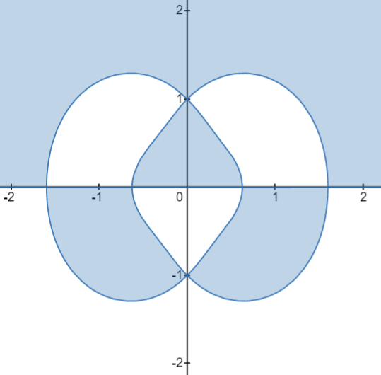
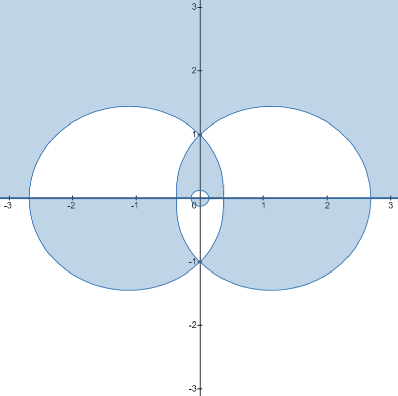
The signature of $\mathrm{Im}k$ are shown in Figure 2. We divide $(y,t)-$half plane into four regions as follows.

• Case I. ${\xi}>2$: No phase point on the real axis, which corresponds to Figure 2 (a);

• Case II. $0<{\xi}<2$: Four phase points on the real axis, which corresponds to Figure 2 (b);

• Case III. $-1/4<{\xi}<0$: Eight phase points on the real axis, which corresponds to Figure 2 (c);

• Case IV. ${\xi}<-1/4$: No phase point on the real axis, which corresponds to Figure 2 (d).

3 Long-time asymptotics in regions without phase point

In this section, we deal with the asymptotic analysis to the Cases I and IV which contain no phase point on the real axis.

3.1 Deformation of the RH problem

The jump matrix $V(k)$ admits two different factorizations

$$V(k) =\left(\begin{array}[]{cc}1&\bar{r}e^{-2it\theta}\\ 0&1\end{array}\right)\left(\begin{array}[]{cc}1&0\\ -re^{2it\theta}&1\end{array}\right)$$ (3.5)

$$=\left(\begin{array}[]{cc}1&0\\ -\frac{re^{2it\theta}}{1-|r|^{2}}&1\end{array}\right)(1-|r|^{2})^{\sigma_{3}}\left(\begin{array}[]{cc}1&\frac{\bar{r}e^{-2it\theta}}{1-|r|^{2}}\\ 0&1\end{array}\right).$$ (3.10)

Denote $\mathcal{N}\triangleq\left\{1,...,4N_{1}+2N_{2}\right\}$ as the subscript set of all poles, and we fix a small positive constant $\delta_{0}$ to give the partitions $\Delta,\nabla$ and $\Lambda$ of $\mathcal{N}$ as follows

$$\Delta=\left\{n\in\mathcal{N}:\text{Im}\theta_{n}>0\right\},\nabla=\left\{n\in\mathcal{N}:\text{Im}\theta_{n}<0\right\},\Lambda=\left\{n\in\mathcal{N}:|\text{Im}\theta_{n}|\leq\delta_{0}\right\},$$ (3.11)

where $\theta_{n}:=\theta(\zeta_{n})$. For $\zeta_{n}$ with $n\in\Delta$, the residue of $M^{J}(k)$ at $\zeta_{n}$ in (2.114) decays to 0 as $t\to\infty$; while for $\zeta_{n}$ with $n\in\nabla$, the residue grows. Denote two constants $\mathcal{N}(\Lambda)=|\Lambda|$ and

$$\rho_{0}=\min_{n\in\mathcal{N}\setminus\Lambda}\left\{|\text{Im}\theta_{n}|\right\}>\delta_{0}.$$ (3.12)

To distinguish different type of zeros, we further give

$$\Delta_{1}=\left\{j\in\left\{1,...,N_{1}\right\}:\text{Im}\theta(\mu_{j})>0\right\},\nabla_{1}=\left\{j\in\left\{1,...,N_{1}\right\}:\text{Im}\theta(\mu_{j})<0\right\},$$

$$\Delta_{2}=\left\{i\in\left\{1,...,N_{2}\right\}:\text{Im}\theta(\nu_{i})>0\right\},\nabla_{2}=\left\{i\in\left\{1,...,N_{2}\right\}:\text{Im}\theta(\nu_{i})<0\right\},$$

$$\Lambda_{1}=\left\{j_{0}\in\left\{1,...,N_{1}\right\}:|\text{Im}\theta(\mu_{j_{0}})|\leq\delta_{0}\right\},\Lambda_{2}=\left\{i_{0}\in\left\{1,...,N_{2}\right\}:|\text{Im}\theta(\nu_{i_{0}})|\leq\delta_{0}\right\}.$$

Introduce a new function

$$T(k)=\prod_{n\in\nabla}\frac{k-\zeta_{n}}{\zeta_{n}^{-1}k-1}\delta(k,\xi),$$ (3.13)

where

$$\delta(k,{\xi})=exp\left\{-i\int_{I(\xi)}\frac{\nu(s)}{s-k}ds\right\},\ \ \ \ \nu(k)=-\frac{1}{2\pi}log(1+|r|^{2}).$$

and

$$I({\xi})=\left\{\begin{array}[]{ll}\emptyset,&\text{as}\ {\xi}>2,\\ \mathbb{R},&\text{as}\ {\xi}<-1/4.\end{array}\right.$$ (3.14)

Besides, define a piecewise matrix function as follows:

$$G(k)=\left\{\begin{array}[]{ll}\left(\begin{array}[]{cc}1&-c_{n}^{-1}(k-\zeta_{n})e^{-2it\theta_{n}}\\ 0&1\end{array}\right),&\text{as }k\in\mathbb{D}_{n},n\in\nabla\setminus\Lambda;\\[12.0pt] \left(\begin{array}[]{cc}1&0\\ -c_{n}(k-\zeta_{n})^{-1}e^{2it\theta_{n}}&1\end{array}\right),&\text{as }k\in\mathbb{D}_{n},n\in\Delta\setminus\Lambda;\\ \left(\begin{array}[]{cc}1&0\\ -\bar{c}_{n}^{-1}(k-\bar{\zeta}_{n})e^{2it\bar{\theta}_{n}}&1\end{array}\right),&\text{as }k\in\overline{\mathbb{D}}_{n},n\in\nabla\setminus\Lambda;\\ \left(\begin{array}[]{cc}1&-\bar{c}_{n}(k-\bar{\zeta}_{n})^{-1}e^{-2it\bar{\theta}_{n}}\\ 0&1\end{array}\right),&\text{as }k\in\overline{\mathbb{D}}_{n},n\in\Delta\setminus\Lambda;\\ I&\text{ elsewhere},\end{array}\right..$$ (3.15)

where $\mathbb{D}_{n}:=\mathbb{D}(\zeta_{n},\varrho)$ with

$$\varrho=\frac{1}{2}\min\left\{\min_{j\in\mathcal{N}}\left\{|\text{Im}\zeta_{j}|\right\},\min_{j\in\mathcal{N}\setminus\Lambda,\text{Im}\theta(k)=0}|\zeta_{j}-k|,\min_{j\in\mathcal{N}}|\zeta_{j}-i|,\min_{j,l\in\mathcal{N}}|\zeta_{j}-\zeta_{l}|\right\}.$$

Now we define a new matrix-valued function $M^{(1)}(z)$ by the following transformation:

$$M^{(1)}(k):=M^{(1)}(y,t,k)=M^{J}(k)G(k)T(k)^{\sigma_{3}},$$ (3.16)

then $M^{(1)}(k)$ has a jump condition on the counter $\Sigma^{(1)}:=\mathbb{R}\cup\left[\underset{n\in\mathcal{N}\setminus\Lambda}{\cup}\left(\partial\overline{\mathbb{D}}_{n}\cup\partial\mathbb{D}_{n}\right)\right]$.

$$M^{(1)}_{+}(k)=M^{(1)}_{-}(k)V^{(1)}(k),\quad k\in\Sigma^{(1)},$$

where

$$V^{(1)}(k)=\left\{\begin{array}[]{ll}\left(\begin{array}[]{cc}1&\bar{r}(k)e^{-2it\theta}T^{-2}(k)\\ 0&1\end{array}\right)\left(\begin{array}[]{cc}1&0\\ -r(k)e^{2it\theta}T^{2}(k)&1\end{array}\right),&\text{as }k\in\mathbb{R}\setminus I(\xi);\\[12.0pt] \left(\begin{array}[]{cc}1&0\\ -\frac{r(k)e^{2it\theta}T^{-2}(k)}{1-|r(k)|^{2}}&1\end{array}\right)\left(\begin{array}[]{cc}1&\frac{\bar{r}(k)e^{-2it\theta}T^{2}(k)}{1-|r(k)|^{2}}\\ 0&1\end{array}\right),&\text{as }k\in I(\xi);\\[12.0pt] \left(\begin{array}[]{cc}1&-c_{n}^{-1}(k-\zeta_{n})T^{-2}(k)e^{-2it\theta_{n}}\\ 0&1\end{array}\right),&\text{as }k\in\partial\mathbb{D}_{n},n\in\nabla\setminus\Lambda;\\[12.0pt] \left(\begin{array}[]{cc}1&0\\ -c_{n}(k-\zeta_{n})^{-1}T^{2}(k)e^{2it\theta_{n}}&1\end{array}\right),&\text{as }k\in\partial\mathbb{D}_{n},n\in\Delta\setminus\Lambda;\\ \left(\begin{array}[]{cc}1&0\\ -\bar{c}_{n}^{-1}(k-\bar{\zeta}_{n})T^{2}(k)e^{2it\bar{\theta}_{n}}&1\end{array}\right),&\text{as }k\in\partial\overline{\mathbb{D}}_{n},n\in\nabla\setminus\Lambda;\\ \left(\begin{array}[]{cc}1&-\bar{c}_{n}(k-\bar{\zeta}_{n})^{-1}T^{-2}(k)e^{-2it\bar{\theta}_{n}}\\ 0&1\end{array}\right),&\text{as }k\in\partial\overline{\mathbb{D}}_{n},n\in\Delta\setminus\Lambda,\\ \end{array}\right.$$ (3.17)

By this transformation, we remove some poles of $M^{J}(k)$, and $M^{(1)}(k)$ only has simple poles at $\zeta_{n}$ and $\bar{\zeta}_{n}$, $n\in\Lambda$ with the following residue condition:

$$\operatorname*{Res}_{k=\zeta_{n}}M^{(1)}(k)=\lim_{k\rightarrow\zeta_{n}}M^{(1)}(k)\left(\begin{array}[]{cc}0&c_{n}^{-1}T^{\prime}\left(\zeta_{n}\right)^{-2}e^{-2it\theta_{n}}\\ 0&0\end{array}\right), n\in\nabla\cap\Lambda,$$ (3.20)

$$\operatorname*{Res}_{k=\zeta_{n}}M^{(1)}(k)=\lim_{k\rightarrow\zeta_{n}}M^{(1)}(k)\left(\begin{array}[]{cc}0&0\\ c_{n}T^{2}\left(\zeta_{n}\right)e^{2it\theta_{n}}&0\end{array}\right), n\in\Delta\cap\Lambda,$$ (3.23)

$$\operatorname*{Res}_{k=\bar{\zeta}_{n}}M^{(1)}(k)=\lim_{k\rightarrow\bar{\zeta}_{n}}M^{(1)}(k)\left(\begin{array}[]{cc}0&0\\ \bar{c}_{n}^{-1}\left(\frac{1}{T}\right)^{\prime}\left(\bar{\zeta}_{n}\right)^{-2}e^{2it\bar{\theta}_{n}}&0\end{array}\right), n\in\nabla\cup\Lambda\text{, }$$ (3.26)

$$\operatorname*{Res}_{k=\overline{\zeta}_{n}}M^{(1)}(k)=\lim_{k\rightarrow\bar{\zeta}_{n}}M^{(1)}(k)\left(\begin{array}[]{cc}0&\bar{c}_{n}T^{-2}\left(\bar{\zeta}_{n}\right)e^{-2it\bar{\theta}_{n}}\\ 0&0\end{array}\right), n\in\Delta\cup\Lambda\text{. }$$ (3.29)

3.2 A mixed $\bar{\partial}$-RH problem

In this part, we make a continuous extension of $V^{(1)}(k)$ to remove the jump from $\mathbb{R}$. First of all, we introduce some new regions and contours:

$$\Omega_{2n+1}=\left\{k\in\mathbb{C}|n\pi\leq\arg k\leq n\pi+\varphi\right\},$$

$$\Omega_{2n+2}=\left\{k\in\mathbb{C}|(n+1)\pi-\varphi\leq\arg k\leq(n+1)\pi\right\},$$

where $n=0,1$ and $0<\varphi<\frac{\pi}{8}$ is a sufficiently small constant. The boundary of $\Omega_{j}$ denote as

$$\Sigma_{j}=e^{(j-1)i\pi/2+i\varphi}\mathbb{R}_{+},\quad j=1,3,$$

$$\Sigma_{j}=e^{ji\pi/2-i\varphi}\mathbb{R}_{+},\qquad\ j=2,4,$$

In addition, let

$$\Omega=\underset{j=1,...,4}{\cup}\Omega_{j},\ \Sigma^{(2)}=\underset{n\in\mathcal{N}\setminus\Lambda}{\cup}\left(\partial\overline{\mathbb{D}}_{n}\cup\partial\mathbb{D}_{n}\right),\ \tilde{\Sigma}=\Sigma_{1}\cup\Sigma_{2}\cup\Sigma_{3}\cup\Sigma_{4}.$$

Introduce the following functions

$$p_{1}(k,\xi)=p_{2}(k,\xi)=\left\{\begin{array}[]{lll}r(k),&\text{ for }\xi>2,\\ -\dfrac{\bar{r}(k)}{1-|r(k)|^{2}},&\text{ for }\ {\xi}<-1/4;\end{array}\right.$$ (3.32)

$$p_{3}(k,\hat{\xi})=p_{4}(k,\hat{\xi})=\left\{\begin{array}[]{lll}\bar{r}(k),&\text{ for}\ {\xi}>2,\\ -\dfrac{r(k)}{1-|r(k)|^{2}},&\text{ for }\ {\xi}<-1/4.\end{array}\right.$$ (3.35)

Then we define a new matrix function $R^{(2)}(k,\xi)$ as:

For ${\xi}\in(2,+\infty)$,

$$R^{(2)}(k,\xi)=\left\{\begin{array}[]{lll}\left(\begin{array}[]{cc}1&R_{j}(k,\xi)e^{-2it\theta}\\ 0&1\end{array}\right),&k\in\Omega_{j},j=1,2;\\ \\ \left(\begin{array}[]{cc}1&0\\ R_{j}(k,\xi)e^{2it\theta}&1\end{array}\right),&z\in\Omega_{j},j=3,4;\\ \\ I,&elsewhere;\\ \end{array}\right.$$ (3.36)

For ${\xi}\in(-\infty,-1/4)$,

$$R^{(2)}(k,\xi)=\left\{\begin{array}[]{lll}\left(\begin{array}[]{cc}1&0\\ R_{j}(k,\xi)e^{2it\theta}&1\end{array}\right),&k\in\Omega_{j},j=1,2;\\ \\ \left(\begin{array}[]{cc}1&R_{j}(k,\xi)e^{-2it\theta}\\ 0&1\end{array}\right),&k\in\Omega_{j},j=3,4;\\ \\ I,&elsewhere,\\ \end{array}\right.$$ (3.37)

where the functions $R_{j}$, $j=1,2,3,4$ are given by the following Proposition.

Proposition 2.

$R_{j}$: $\bar{\Omega}_{j}\to\mathbb{C}$, $j=1,2,3,4$ have boundary values as follows:

$$R_{1}(k,\xi)=\Bigg{\{}\begin{array}[]{ll}p_{1}(k,\xi)T(k)^{-2}&k\in\mathbb{R}^{+},\\ 0&k\in\Sigma_{1},\\ \end{array},\hskip 17.07182ptR_{2}(k,\xi)=\Bigg{\{}\begin{array}[]{ll}0&k\in\Sigma_{2},\\ p_{2}(k,\xi)T(k)^{-2}&k\in\mathbb{R}^{-},\\ \end{array}$$ (3.42)

$$R_{3}(k,\xi)=\Bigg{\{}\begin{array}[]{ll}p_{3}(k,\xi)T(k)^{2}&k\in\mathbb{R}^{-},\\ 0&k\in\Sigma_{3},\\ \end{array},\hskip 17.07182ptR_{4}(k,\xi)=\Bigg{\{}\begin{array}[]{ll}0&k\in\Sigma_{4},\\ p_{4}(k,\xi)T(k)^{2}&k\in\mathbb{R}^{+},\\ \end{array}$$ (3.47)

$R_{j}$ admit the following property: for $j=1,2,3,4,$

$$|\bar{\partial}R_{j}(k)|\lesssim|r^{\prime}(|k|)|+|k|^{-1/2},\ \text{for all $k\in\Omega_{j}$,}$$ (3.48)

and

$$|\bar{\partial}R_{j}(k)|\lesssim|r^{\prime}(|k|)|+|k|^{-1},\ \text{for all $k\in\Omega_{j}$.}$$ (3.49)

$$\bar{\partial}R_{j}(k)=0,\hskip 14.22636pt\text{for all }k\in elsewhere.$$

Using $R^{(2)}(k)$, we define the new transformation

$$M^{(2)}(k):=M^{(2)}(y,t,k)=M^{(1)}(k)R^{(2)}(k),$$ (3.50)

then $M^{(2)}(k)$ satisfies a mixed $\bar{\partial}$-RH problem with the jump condition

$$M^{(2)}_{+}(k)=M^{(2)}_{-}(k)V^{(2)}(k),\quad k\in\Sigma^{(2)},$$ (3.51)

where

$$V^{(2)}(k)=\left\{\begin{array}[]{ll}\left(\begin{array}[]{cc}1&-c_{n}^{-1}(k-\zeta_{n})T^{-2}(k)e^{-2it\theta_{n}}\\ 0&1\end{array}\right),&\text{as }k\in\partial\mathbb{D}_{n},n\in\nabla\setminus\Lambda;\\[12.0pt] \left(\begin{array}[]{cc}1&0\\ -c_{n}(k-\zeta_{n})^{-1}T^{2}(k)e^{2it\theta_{n}}&1\end{array}\right),&\text{as }k\in\partial\mathbb{D}_{n},n\in\Delta\setminus\Lambda;\\ \left(\begin{array}[]{cc}1&0\\ -\bar{c}_{n}^{-1}(k-\bar{\zeta}_{n})T^{2}(k)e^{2it\bar{\theta}_{n}}&1\end{array}\right),&\text{as }k\in\partial\overline{\mathbb{D}}_{n},n\in\nabla\setminus\Lambda;\\ \left(\begin{array}[]{cc}1&-\bar{c}_{n}(k-\bar{\zeta}_{n})^{-1}T^{-2}(k)e^{-2it\bar{\theta}_{n}}\\ 0&1\end{array}\right),&\text{as }k\in\partial\overline{\mathbb{D}}_{n},n\in\Delta\setminus\Lambda.\\ \end{array}\right.$$ (3.52)

and the $\bar{\partial}-$ derivative

$$\bar{\partial}M^{(2)}(k)=M^{(2)}(k)\bar{\partial}R^{(2)}(k),$$ (3.53)

where for ${\xi}\in(2,+\infty)$,

$$\bar{\partial}R^{(2)}(k,\hat{\xi})=\left\{\begin{array}[]{lll}\left(\begin{array}[]{cc}0&\bar{\partial}R_{j}(k,\hat{\xi})e^{-2it\theta}\\ 0&0\end{array}\right),&k\in\Omega_{j},j=1,2;\\ \\ \left(\begin{array}[]{cc}0&0\\ \bar{\partial}R_{j}(k,\hat{\xi})e^{2it\theta}&0\end{array}\right),&z\in\Omega_{j},j=3,4;\\ \\ 0,&elsewhere;\\ \end{array}\right.$$ (3.54)

for ${\xi}\in(-\infty,-1/4)$,

$$\bar{\partial}R^{(2)}(k,\xi)=\left\{\begin{array}[]{lll}\left(\begin{array}[]{cc}0&0\\ \bar{\partial}R_{j}(k,\xi)e^{2it\theta}&0\end{array}\right),&k\in\Omega_{j},j=1,2;\\ \\ \left(\begin{array}[]{cc}0&\bar{\partial}R_{j}(k,\xi)e^{-2it\theta}\\ 0&0\end{array}\right),&k\in\Omega_{j},j=3,4;\\ \\ 0,&elsewhere.\\ \end{array}\right.$$ (3.55)

To solve this mixed $\bar{\partial}-$RH problem, we decompose it into a pure RH problem for $M^{R}(k)$ and a pure $\bar{\partial}-$Problem. Firstly, we introduce a new function $M^{R}(k):=M^{R}(y,t,k)$ satisfying a pure RH problem

RHP 3.

Find a matrix-valued function $M^{R}(z)$ with following properties:

• Analyticity: $M^{R}(k)$ is meromorphic in $\mathbb{C}\setminus\Sigma^{(2)}$;

• Asymptotic behavior:

  $$M^{R}(k)= I+\mathcal{O}(k^{-1}),\hskip 14.22636ptk\rightarrow\infty;$$ (3.56)

• Jump condition: $M^{R}(k)$ has continuous boundary values $M^{R}_{\pm}(k)$ on $\Sigma^{(2)}$ and

  $$M^{R}_{+}(k)=M^{R}_{-}(k)V^{(2)}(k),\quad k\in\Sigma^{(2)};$$ (3.57)

• $\bar{\partial}$-Derivative: $\bar{\partial}R^{(2)}(k)=0,$ for all $k\in\mathbb{C}$;

• Residue conditions: $M^{R}(k)$ has simple poles at each point $\zeta_{n}$ and $\bar{\zeta}_{n}$ for $n\in\Lambda$ with

  $$\operatorname*{Res}_{k=\zeta_{n}}M^{R}(k)=\lim_{k\rightarrow\zeta_{n}}M^{R}(k)\left(\begin{array}[]{cc}0&c_{n}^{-1}T^{\prime}\left(\zeta_{n}\right)^{-2}e^{-2it\theta_{n}}\\ 0&0\end{array}\right), n\in\nabla\cap\Lambda,$$

  $$\operatorname*{Res}_{k=\zeta_{n}}M^{R}(k)=\lim_{k\rightarrow\zeta_{n}}M^{R}(k)\left(\begin{array}[]{cc}0&0\\ c_{n}T^{2}\left(\zeta_{n}\right)e^{2it\theta_{n}}&0\end{array}\right), n\in\Delta\cap\Lambda,$$

  $$\operatorname*{Res}_{k=\bar{\zeta}_{n}}M^{R}(k)=\lim_{k\rightarrow\bar{\zeta}_{n}}M^{R}(k)\left(\begin{array}[]{cc}0&0\\ \bar{c}_{n}^{-1}\left(\frac{1}{T}\right)^{\prime}\left(\bar{\zeta}_{n}\right)^{-2}e^{2it\bar{\theta}_{n}}&0\end{array}\right), n\in\nabla\cup\Lambda\text{, }$$

  $$\operatorname*{Res}_{k=\overline{\zeta}_{n}}M^{R}(k)=\lim_{k\rightarrow\bar{\zeta}_{n}}M^{R}(k)\left(\begin{array}[]{cc}0&\bar{c}_{n}T^{-2}\left(\bar{\zeta}_{n}\right)e^{-2it\bar{\theta}_{n}}\\ 0&0\end{array}\right), n\in\Delta\cup\Lambda\text{. }$$

We then use $M^{R}(k)$ to construct a new matrix function

$$M^{(3)}(k):=M^{(2)}(k)M^{R}(k)^{-1},$$ (3.58)

which is a pure $\bar{\partial}-$problem with

$$\bar{\partial}M^{(3)}(k)=M^{(3)}(k)W^{(3)}(k),\ \ k\in\mathbb{C},$$

where

$$W^{(3)}(k)=M^{R}(k)\bar{\partial}R^{(2)}(k)M^{R}(k)^{-1}.$$ (3.59)

3.3 Contribution from a pure RH problem

In this part, we finish the asymptotic analysis of $M^{R}(k)$. By simple proof, we find the jump matrix $V^{(2)}(k)$ satisfies the estimates: for $1\leq\tilde{p}\leq\infty,$

$$\parallel V^{(2)}(k)-I\parallel_{L^{\tilde{p}}(\Sigma^{(2)})}=\mathcal{\mathcal{O}}(e^{-2\rho_{0}t}),$$ (3.60)

where $\rho_{0}$ is given in (3.12). Now we decompose $M^{R}(k)$ as

$$M^{R}(k)=\tilde{E}(k)M^{(r)}_{\Lambda}(k),$$ (3.61)

where $\tilde{E}(k)$ is an error function, and $M^{(r)}_{\Lambda}$ satisfies a new RH problem:

RHP 4.

Find a matrix-valued function $M^{(r)}_{\Lambda}(k)$ with the following properties:

• Analyticity: $M^{(r)}_{\Lambda}(k)$ is analytical in $\mathbb{C}\setminus\left\{\zeta_{n},\bar{\zeta}_{n}\right\}_{n\in\Lambda}$;

• Asymptotic behaviors:

  $$M^{(r)}_{\Lambda}(k)=I+\mathcal{O}(k^{-1}),\quad k\rightarrow\infty;$$ (3.62)

• Residue conditions: $M^{(r)}_{\Lambda}(k)$ has simple poles at each point $\zeta_{n}$ and $\bar{\zeta}_{n}$ for $n\in\Lambda$ with:

  $$\operatorname*{Res}_{k=\zeta_{n}}M^{(r)}_{\Lambda}(k)=\lim_{k\rightarrow\zeta_{n}}M^{(r)}_{\Lambda}(k)\left(\begin{array}[]{cc}0&c_{n}^{-1}T^{\prime}\left(\zeta_{n}\right)^{-2}e^{-2it\theta_{n}}\\ 0&0\end{array}\right), n\in\nabla\cap\Lambda,$$ (3.65)

  $$\operatorname*{Res}_{k=\zeta_{n}}M^{(r)}_{\Lambda}(k)=\lim_{k\rightarrow\zeta_{n}}M^{(r)}_{\Lambda}(k)\left(\begin{array}[]{cc}0&0\\ c_{n}T^{2}\left(\zeta_{n}\right)e^{2it\theta_{n}}&0\end{array}\right), n\in\Delta\cap\Lambda,$$ (3.68)

  $$\operatorname*{Res}_{k=\bar{\zeta}_{n}}M^{(r)}_{\Lambda}(k)=\lim_{k\rightarrow\bar{\zeta}_{n}}M^{(r)}_{\Lambda}(k)\left(\begin{array}[]{cc}0&0\\ \bar{c}_{n}^{-1}\left(\frac{1}{T}\right)^{\prime}\left(\bar{\zeta}_{n}\right)^{-2}e^{2it\bar{\theta}_{n}}&0\end{array}\right), n\in\nabla\cup\Lambda\text{, }$$ (3.71)

  $$\operatorname*{Res}_{k=\overline{\zeta}_{n}}M^{(r)}_{\Lambda}(k)=\lim_{k\rightarrow\bar{\zeta}_{n}}M^{(r)}_{\Lambda}(k)\left(\begin{array}[]{cc}0&\bar{c}_{n}T^{-2}\left(\bar{\zeta}_{n}\right)e^{-2it\bar{\theta}_{n}}\\ 0&0\end{array}\right), n\in\Delta\cup\Lambda\text{. }$$ (3.74)

It has been proved that there exists an unique solution $M^{(r)}_{\Lambda}(k)$ of the RH problem 7, and $M^{(r)}_{\Lambda}(k)$ is solvable as a reflectionless solution of the original RH problem.

At the end of this part, we estimate the error between $M^{R}(k)$ and $M^{(r)}_{\Lambda}$, that is $\tilde{E}(k)$, which solves a small norm RH problem:

RHP 5.

Find a matrix-valued function $\tilde{E}(k)$ admitting the following identities:

• Analyticity: $\tilde{E}(k)$ is analytical in $\mathbb{C}\setminus\Sigma^{(2)}$;

• Asymptotic behavior:

  $$\tilde{E}(k)\sim I+\mathcal{O}(k^{-1}),\hskip 14.22636ptk\rightarrow\infty;$$ (3.75)

• Jump condition: $\tilde{E}(k)$ has continuous boundary values $\tilde{E}_{\pm}(k)$ on $\Sigma^{(2)}$ with

  $$\tilde{E}_{+}(k)=\tilde{E}_{-}(k)V^{\tilde{E}}(k),$$

  where

  $$V^{\tilde{E}}(k)=M^{(r)}_{\Lambda}(k)V^{(2)}(k)M^{(r)}_{\Lambda}(k)^{-1}.$$ (3.76)

The existence and uniqueness of this RH problem is proved by using a small-norm RH problem [34, 35] with the Cauchy projection operator.

To reconstruct the solutions $p,q$, we deduce the asymptotic behavior of $\tilde{E}(k)$ at $k=i$ and give the estimates:

Proposition 3.

The matrix function $\tilde{E}(k)$ satisfies the estimates:

$$|\tilde{E}(k)-I|\lesssim\mathcal{O}(e^{-2\rho_{0}t}).$$ (3.77)

Besides, as $k\to i$, $\tilde{E}(k)$ has the expansion

$$\tilde{E}(k)=\tilde{E}(i)+\tilde{E}_{1}(k-i)+\mathcal{O}((k-i)^{2}),$$ (3.78)

$\tilde{E}(i)$ and $\tilde{E}_{1}$ satisfy the following long time asymptotic condition:

$$|\tilde{E}(i)-I|\lesssim\mathcal{O}(e^{-2\rho_{0}t}),\hskip 14.22636pt\tilde{E}_{1}\lesssim\mathcal{O}(e^{-2\rho_{0}t}).$$ (3.79)

3.4 Contribution from a pure $\bar{\partial}$-problem

Now we consider the asymptotic behavior of $M^{(3)}(k)$ defined by (3.58). The solution of the $\bar{\partial}$-problem for $M^{(3)}(k)$ is equivalent to the integral equation

$$M^{(3)}(k)=I+\frac{1}{\pi}\iint_{\mathbb{C}}\dfrac{M^{(3)}(s)W^{(3)}(s)}{s-k}dm(s),$$ (3.80)

where $m(s)$ is the Lebesgue measure on $\mathbb{C}$. Define $C_{k}$ as the left Cauchy integral operator

$$fC_{k}(k)=\frac{1}{\pi}\iint_{C}\dfrac{f(s)W^{(3)}(s)}{s-k}dm(s).$$

Then (3.80) can be rewritten as

$$M^{(3)}(k)=I\cdot\left(I-C_{k}\right)^{-1}.$$ (3.81)

Therefore, the existence of the solution $M^{(3)}(k)$ is guaranteed by the estimates:

$$\parallel C_{k}\parallel_{L^{\infty}\to L^{\infty}}\lesssim t^{-1/2}.$$

Take $k=i$ in (3.80), then

$$M^{(3)}(i)=I+\frac{1}{\pi}\iint_{\mathbb{C}}\dfrac{M^{(3)}(s)W^{(3)}(s)}{s-i}dm(s).$$ (3.82)

To reconstruct the solution of (1.8)-(1.9), we derive the following proposition.

Proposition 4.

There exist a small positive constant $\rho<1/4$, such that the solution $M^{(3)}(k)$ of $\bar{\partial}$-problem admits the following estimation

$$\parallel M^{(3)}(i)-I\parallel=\parallel\frac{1}{\pi}\iint_{\mathbb{C}}\dfrac{M^{(3)}(s)W^{(3)}(s)}{s-i}dm(s)\parallel\lesssim t^{-1+2\rho}.$$ (3.83)

As $k\to i$, $M^{(3)}(k)$ has asymptotic expansion

$$M^{(3)}(k)=M^{(3)}(i)+M^{(3)}_{1}(y,t)(k-i)+\mathcal{O}((k-i)^{2}),$$ (3.84)

where $M^{(3)}_{1}(y,t)$ is a $k$-independent coefficient with

$$M^{(3)}_{1}(y,t)=\frac{1}{\pi}\iint_{C}\dfrac{M^{(3)}(s)W^{(3)}(s)}{(s-i)^{2}}dm(s).$$ (3.85)

There exist constants $T_{1}$, such that for all $t>T_{1}$, $M^{(3)}_{1}(y,t)$ satisfies

$$|M^{(3)}_{1}(y,t)|\lesssim t^{-1+2\rho}.$$ (3.86)

3.5 Proof of Theorem 1–Case I.

Before the long-time asymptotics, we deal with several coefficient matrix in the transformations above. We first denote

$$F(k):=\left(I+\frac{\sigma_{1}}{k}\right)^{-1}\left(I+\frac{\sigma_{1}M^{J}(0)^{-1}}{k}\right).$$ (3.87)

By simple calculation, $F(k)$ has the following expansion at $k=i$

$$F(k)=F_{1}+F_{2}(k-i)+O((k-i)^{2})+O(t^{-1/2}),$$ (3.88)

where

$$F_{j}=\left(\begin{array}[]{cc}F_{j1}&F_{j2}\\ F_{j3}&F_{j4}\end{array}\right),\quad j=1,2$$ (3.89)

are constant matrix. Besides, $T(k)$ has the following asymptotic expansion at $k=i$:

$$T(k)=T_{0}+T_{1}(k-i)+\mathcal{O}((k-i)^{2}).$$ (3.90)

Now we begin to construct the long-time asymptotics for solutions of the 2-mCH equation (1.8)-(1.9). Inverting all above transformations (2.110), (3.16), (3.50), (3.58) and (3.61), we have

$$M(k)= F(k)M^{(3)}(k)\tilde{E}(k)M^{R}(k)R^{(2)}(k)^{-1}T(k)^{-\sigma_{3}}.$$ (3.91)

To reconstruct $p(x,t),q(x,t)$ by using (2.105), we take $z\to i$ along the path out of $\bar{\Omega}$. In this case, $R^{(2)}(k)=I$. Further using Propositions 3 and 4, we obtain that as $k\to i$

$$M(k)=\left(\begin{array}[]{cc}f_{11}(y,t,k)&f_{12}(y,t,k)\\ f_{21}(y,t,k)&f_{22}(y,t,k)\end{array}\right)+\mathcal{O}((k-i)^{2})+\mathcal{O}(t^{-1+2\rho}),$$ (3.94)

where

$$f_{11}:= \left(F_{11}M_{\Lambda,11}^{(r)}(i)+F_{12}M_{\Lambda,21}^{(r)}(i)\right)T_{0}^{-1}$$

$$+\left[\left(F_{11}M_{\Lambda,11}^{(r)}(i)+F_{12}M_{\Lambda,21}^{(r)}(i)\right)T_{1}^{-1}+\left(F_{21}M_{\Lambda,11}^{(r)}(i)+F_{22}M_{\Lambda,21}^{(r)}(i)\right)T_{0}^{-1}\right](k-i),$$

$$f_{12}:= \left(F_{11}M_{\Lambda,12}^{(r)}(i)+F_{22}M_{\Lambda,22}^{(r)}(i)\right)T_{0}$$

$$+\left[\left(F_{11}M_{\Lambda,12}^{(r)}(i)+F_{12}M_{\Lambda,22}^{(r)}(i)\right)T_{1}+\left(F_{21}M_{\Lambda,12}^{(r)}(i)+F_{22}M_{\Lambda,22}^{(r)}(i)\right)T_{0}\right](k-i),$$

$$f_{21}:= \left(F_{13}M_{\Lambda,11}^{(r)}+F_{14}M_{\Lambda,21}^{(r)}\right)T_{0}^{-1}$$

$$+\left[\left(F_{13}M_{\Lambda,11}^{(r)}(i)+F_{14}M_{\Lambda,21}^{(r)}(i)\right)T_{1}^{-1}+\left(F_{23}M_{\Lambda,11}^{(r)}(i)+F_{24}M_{\Lambda,21}^{(r)}(i)\right)T_{0}^{-1}\right](k-i),$$

$$f_{22}:= \left(F_{13}M_{\Lambda,12}^{(r)}(i)+F_{14}M_{\Lambda,22}^{(r)}(i)\right)T_{0}$$

$$+\left[\left(F_{13}M_{\Lambda,12}^{(r)}(i)+F_{14}M_{\Lambda,22}^{(r)}(i)\right)T_{1}\quad\left(F_{23}M_{\Lambda,12}^{(r)}(i)+F_{24}M_{\Lambda,22}^{(r)}(i)\right)T_{0}\right](k-i).$$

Substituting the expansion of each component of $M(k)$ into the reconstruction formula (2.105), we further get the long-time asymptotic behavior for solutions of the 2-mCH equation (1.8)-(1.9) in the case without stationary phase point.

4 Long-time asymptotics in regions with phase points

In this section, we study the long-time asymptotic behavior for the solutions of 2-mCH equation (1.8)-(1.9) in the cases II and III. For convenience, we introduce a function $n({\xi})$ to show the number of stationary phase points

$$n({\xi})=\left\{\begin{array}[]{l}4,\qquad 0<0{\xi}<2,\\ 8,\qquad-1/4<{\xi}<0,\end{array}\right.$$ (4.3)

and define several lines divided by the stationary phase points:

for $0<{\xi}<2$,

$$I_{j1}=I_{j2}=\left\{\begin{array}[]{ll}\left(\frac{k_{j}+k_{j+1}}{2},k_{j}\right),&j\text{ is odd },\\[10.0pt] \left(k_{j},\frac{k_{j}+k_{j-1}}{2}\right),&j\text{ is even },\end{array}\right.$$ (4.6)

$$I_{j3}=I_{j4}=\left\{\begin{array}[]{ll}\left(k_{j},\frac{k_{j}+k_{j-1}}{2}\right),&j\text{ is odd},\\[10.0pt] \left(\frac{k_{j}+k_{j+1}}{2},k_{j}\right),&j\text{ is even};\end{array}\right.$$ (4.9)

for $-1/4<{\xi}<0$,

$$I_{j1}=I_{j2}=\left\{\begin{array}[]{ll}\left(k_{j},\frac{k_{j}+k_{j-1}}{2}\right),&j\text{ is odd},\\[10.0pt] \left(\frac{k_{j}+k_{j+1}}{2},k_{j}\right),&j\text{ is even},\end{array}\right.$$ (4.12)

$$I_{j3}=I_{j4}=\left\{\begin{array}[]{ll}\left(\frac{k_{j}+k_{j+1}}{2},k_{j}\right),&j\text{ is odd},\\[10.0pt] \left(k_{j},\frac{k_{j}+k_{j-1}}{2}\right),&j\text{ is even}.\end{array}\right.$$ (4.15)

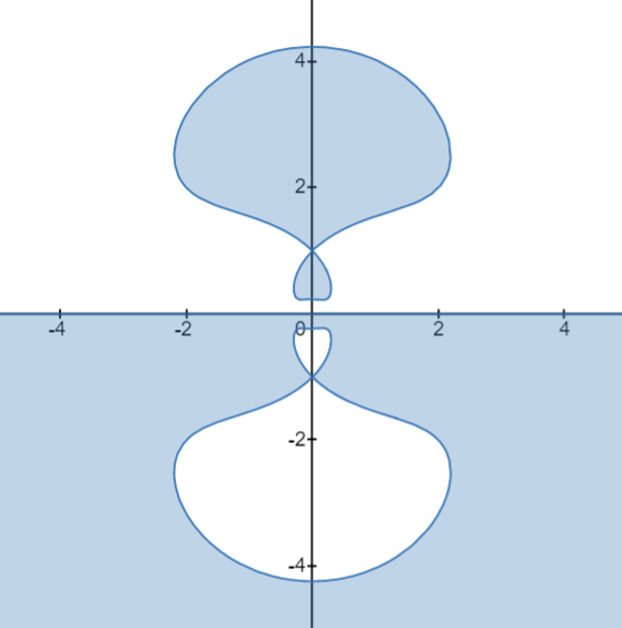
where $k_{j}$ are the stationary points in the two cases as shown in Figure 3.

Figure 3: Figure (a) and (b) are corresponding to the case $0<{\xi}<2$ and $-1/4<{\xi}<0$ respectively. In (a), there are four stationary phase points $k_{1},...k_{4}$ with $k_{1}=-k_{4}=k_{2}^{-1}=-k_{3}^{-1}$. And in (b), there are eight stationary phase points $k_{1},...k_{8}$ with $k_{1}=-k_{8}=k_{4}^{-1}=-k_{5}^{-1}$ and $k_{2}=-k_{7}=k_{3}^{-1}=-k_{6}^{-1}$.

4.1 Deformation of the RH problem

Take a transformation

$$M^{(1)}(k):=M^{J}(k)G(k)T(k)^{\sigma_{3}},$$ (4.16)

where $T(k)$ and $G(k)$ are given by (3.13) and (3.15) with

$$I({\xi})=\left\{\begin{array}[]{ll}\left(k_{1},k_{2}\right)\cup\left(k_{3},k_{4}\right),&0<{\xi}<2,\\ \left(k_{2},k_{3}\right)\cup\left(k_{4},k_{5}\right)\cup\left(k_{6},k_{7}\right),&-1/4<{\xi}<0.\end{array}\right.$$ (4.19)

Then $M^{(1)}(k)$ solves a new RH problem with the jump condition

$$M^{(1)}_{+}(k)=M^{(1)}_{-}(k)V^{(1)}(k),\quad k\in\Sigma^{(1)},$$

where $V^{(1)}(k)$ is defined by (3.17), and $M^{(1)}(k)$ satisfies the residue condition (3.20)-(3.29).

For the cases of ${\xi}\in(-1/4,0)\cup(0,2)$, there exists stationary phase points on the real axis. To discuss the asymptotic behavior of the RH problem near these points, we add a property related to $T(k)$:

As $k\to k_{j}$ along the ray $k_{j}+e^{i\phi}\mathbb{R}^{+}$ with $|\phi|<\pi$ ,

$$|T(k,{\xi})-T_{j}(\xi)\left(\eta(\xi,k_{j})(k-k_{j})\right)^{\eta(\xi,k_{j})i\nu(k_{j})}|\lesssim\parallel r\parallel_{H^{1}(\mathbb{R})}|k-k_{j}|^{1/2},$$ (4.20)

where

$$\eta({\xi},k_{j})=\left\{\begin{array}[]{ll}(-1)^{j},&\text{as }-1/4<{\xi}<0;\\ (-1)^{j+1},&\text{as }0<{\xi}<2,\ \ j=1,\cdots,n(\xi).\end{array}\right.$$ (4.23)

$T_{j}(\xi)$ is defined as

$$T_{j}(\xi)=\prod_{n\in\Delta}\dfrac{k-\zeta_{n}}{\bar{\zeta}_{n}^{-1}k-1}e^{i\beta_{j}(k_{j},\xi)}$$ (4.24)

and

$$\beta_{j}(k,\xi)=\int_{I(\xi)}\frac{\nu(s)}{s-k}ds-\eta(\xi,k_{j})\log\left(\eta(\xi,k_{j})(k-k_{j})\right)\nu(k_{j}),$$ (4.25)

for $j=1,...,n(\xi)$.

4.2 A mixed $\bar{\partial}$-RH problem

In this part, we make a continuous extension of $V^{(1)}(k)$ to remove the jump from $\mathbb{R}$. We first define deformation contours and domains:

For $j=2,...,n(\xi)-1$,

$$\Sigma_{jl}(\xi)=\left\{\begin{array}[]{lll}k_{j}+e^{i[(l/2+1/2+j)\pi+(-1)^{j+1}\varphi]}l_{0},&\ -1/4<{\xi}<0,\\[5.0pt] k_{j}+e^{i[(l/2+j)\pi+(-1)^{j}\varphi]}l_{0},&\ 0<{\xi}<2,\end{array}\right.\hskip 5.69046ptl=1,3,$$ (4.28)

$$\Sigma_{jl}(\hat{\xi})=\left\{\begin{array}[]{lll}k_{j}+e^{i[(l/2+j)\pi+(-1)^{j}\varphi]}l_{0},&\ -1/4<{\xi}<0,\\[5.0pt] k_{j}+e^{i[(k/2+1/2+j)\pi+(-1)^{j+1}\varphi]}l_{0},&\ 0<{\xi}<2,\end{array}\right.\hskip 5.69046ptl=2,4,$$ (4.31)

For $j=1,n(\xi)$,

$$\Sigma_{j1}(\xi)=\left\{\begin{array}[]{lll}k_{j}+e^{(1+j)\pi i+(-1)^{j+1}i\varphi}\mathbb{R}^{+},&\ -1/4<{\xi}<0,\\[5.0pt] k_{j}+e^{j\pi i+(-1)^{j}i\varphi}l_{0},&\ 0<{\xi}<2,\end{array}\right.$$ (4.34)

$$\Sigma_{j2}(\xi)=\left\{\begin{array}[]{lll}k_{j}+e^{(1+j)\pi i+(-1)^{j}i\varphi}\mathbb{R}^{+},&0<{\xi}<2,\\[5.0pt] k_{j}+e^{j\pi i+(-1)^{j+1}i\varphi}l_{0},&\ 0<{\xi}<2,\end{array}\right.$$ (4.37)

$$\Sigma_{j3}(\xi)=\left\{\begin{array}[]{lll}k_{j}+e^{j\pi i+(-1)^{j+1}i\varphi}l_{0},&\ 0<{\xi}<2,\\[5.0pt] k_{j}+e^{(1+j)\pi i+(-1)^{j}i\varphi}\mathbb{R}^{+},&\ 0<{\xi}<2,\end{array}\right.$$ (4.40)

$$\Sigma_{j4}(\xi)=\left\{\begin{array}[]{lll}k_{j}+e^{j\pi i+(-1)^{j}i\varphi}l_{0},&\ -1/4<{\xi}<0,\\[5.0pt] k_{j}+e^{(1+j)\pi i+(-1)^{j+1}i\varphi}\mathbb{R}^{+},&\ 0<{\xi}<2.\end{array}\right.$$ (4.43)

$$\Sigma_{j\pm}^{\prime}=\left\{\begin{array}[]{lll}\frac{k_{j+1}+k_{j}}{2}+e^{i\pi}l_{0},&\ -1/4<{\xi}<0,\ j=1,...,n(\xi)-1,\\ \frac{k_{j-1}+k_{j}}{2}-e^{i\pi}l_{0},&\ 0<{\xi}<2,\ j=2,...,n(\xi).\end{array}\right.$$ (4.46)

where $l_{0}\in(0,\frac{|k_{j+(-1)^{j}}-k_{j}|}{2\cos\varphi})$, $\varphi$ is an fixed sufficiently small angle. For convenience, denote $\Sigma_{n(\xi)\pm}^{\prime}=\emptyset$ as $-1/4<\xi<0$ and $\Sigma_{1\pm}^{\prime}=\emptyset$ as $0<{\xi}<2$. We further denote

$$\tilde{\Sigma}(\xi)=\left(\underset{j=1,..,n(\xi)}{\underset{l=1,...,4,}{\cup}}\Sigma_{jl}\right)\bigcup\left(\underset{j=1,...,n(\xi)}{\cup}\Sigma^{\prime}{j\pm}\right),\hskip 14.22636pt$$

$$\Sigma^{(2)}(\xi)=\tilde{\Sigma}(\xi)\underset{n\in\mathcal{N}\setminus\Lambda}{\cup}\left(\partial\overline{\mathbb{D}}_{n}\cup\partial\mathbb{D}_{n}\right),$$

$$\Omega(\xi)=\underset{j=1,..,n(\xi)}{\underset{l=1,...,4,}{\cup}}\Omega_{jl},\hskip 14.22636pt\Omega_{\pm}(\xi)=\mathbb{C}\setminus\Omega.$$

Introduce a new unknown function

$$R^{(2)}(k,\xi)=\left\{\begin{array}[]{lll}\left(\begin{array}[]{cc}1&R_{jl}(k,\xi)e^{-2it\theta}\\ 0&1\end{array}\right),&k\in\Omega_{jl},\ j=1,...,n(\xi),\ l=1,3;\\ \\ \left(\begin{array}[]{cc}1&0\\ R_{jl}(k,\xi)e^{2it\theta}&1\end{array}\right),&k\in\Omega_{jl},\ j=1,...,n(\xi),\ l=2,4;\\ \\ I,&elsewhere;\\ \end{array}\right.$$ (4.47)

where the functions $R_{jl}(k,\xi)$, $j=1,...,n(\xi)$, $l=1,2,3,4$ are defined to satisfy the following properties:

Proposition 5.

For $\xi\in(-1/4,0)$ and ${\xi}\in(0,2)$, the functions $R_{jl}$: $\bar{\Omega}_{jl}\to\mathbb{C}$, $l=1,2,3,4$, $j=1,...,n(\xi)$ have the boundary values:

$$R_{j1}(k,\xi)=\left\{\begin{array}[]{ll}p_{j1}(k,\xi)T_{+}(k)^{2},&\hskip 11.38092ptk\in I_{j1},\\ p_{j1}(k_{j},\xi)T_{j}(\xi)^{2}(\eta(\xi,k_{j})(k-k_{j}))^{2i\nu(k_{j})},&\hskip 11.38092ptk\in\Sigma_{j1},\\ \end{array}\right.$$ (4.50)

$$R_{j2}(k,\xi)=\left\{\begin{array}[]{ll}p_{j2}(k_{j},\xi)T_{j}(\xi)^{-2}(\eta(\xi,k_{j})(k-k_{j}))^{-2i\nu(k_{j})},&k\in\Sigma_{j2},\\ p_{j2}(k,\xi)T_{-}(k)^{-2},&k\in I_{j2},\\ \end{array}\right.$$ (4.53)

$$R_{j3}(k,\xi)=\left\{\begin{array}[]{ll}p_{j3}(k,\xi)T(k)^{2},&\hskip 11.38092ptk\in I_{j3},\\ p_{j3}(k_{j},\xi)T_{j}(\xi)^{2}(\eta(\xi,k_{j})(k-k_{j}))^{2i\nu(k_{j})},&\hskip 11.38092ptk\in\Sigma_{j3},\\ \end{array}\right.$$ (4.56)

$$R_{j4}(k,\xi)=\left\{\begin{array}[]{ll}p_{j4}(k_{j},\xi)T_{j}(\xi)^{-2}(\eta(\xi,k_{j})(k-k_{j}))^{-2i\nu(k_{j})},&k\in\Sigma_{j4},\\ p_{j4}(k,\xi)T(k)^{-2},&k\in I_{j4},\end{array}\right.$$ (4.59)

where $I_{jl}$ are defined by (4.6)-(4.15) and

$$p_{j1}(k,\xi)=-\dfrac{\bar{r}(k)}{1-|r(k)|^{2}},\ p_{j2}(k,\xi)=-\dfrac{r(k)}{1-|r(k)|^{2}},\ p_{j3}(k,\xi)=\bar{r}(k),\ p_{j4}(k,\xi)=r(k).$$ (4.60)

The functions $R_{jl}(k)$ admit the following estimates:

$$|R_{jl}(k,\xi)|\lesssim\sin^{2}(\frac{\pi\arg(k-k_{j})}{2\varphi})+\left(1+\text{Re}(k)^{2}\right)^{-1/2},\quad\text{for all $k\in\Omega_{jl}$},$$ (4.61)

$$|\bar{\partial}R_{jl}(k,\hat{\xi})|\lesssim|r^{\prime}(\text{Re}k)|+|k-k_{j}|^{-1/2},\quad\text{for all $k\in\Omega_{jl}$,}$$ (4.62)

$$\bar{\partial}R_{jl}(k,\xi)=0,\hskip 14.22636ptelsewhere.$$ (4.63)

Define a new matrix function using $R^{(2)}(k)$ as

$$M^{(2)}(k):=M^{(2)}(y,t,k)=M^{(1)}(k)R^{(2)}(k).$$ (4.64)

Then $M^{(2)}(k)$ satisfies a mixed $\bar{\partial}-$RH problem with the jump condition

$$M^{(2)}_{+}(k)=M^{(2)}_{-}(k)V^{(2)}(k),\quad k\in\Sigma^{(2)},$$ (4.65)

where

$$V^{(2)}(k)=\left\{\begin{array}[]{ll}R^{(2)}(k)|_{\Sigma_{j1}\cup\Sigma_{j4}},&\text{as }k\in\Sigma_{j1}\cup\Sigma_{j4};\\[12.0pt] R^{(2)}(k)^{-1}|_{\Sigma_{j2}\cup\Sigma_{j3}},&\text{as }k\in\Sigma_{j2}\cup\Sigma_{j3};\\[12.0pt] R^{(2)}(k)^{-1}|_{\Sigma_{j\ (3\pm 1)/2}}R^{(2)}(k)|_{\Sigma_{(j-1)\ (3\pm 1)/2}},&\text{as }k\in\Sigma_{j\pm}^{\prime},\ j\text{ is even};\\[12.0pt] R^{(2)}(k)^{-1}|_{\Sigma_{j\ (7\pm 1)/2}}R^{(2)}(k)|_{\Sigma_{(j-1)\ (7\pm 1)/2}},&\text{as }k\in\Sigma_{j\pm}^{\prime},\ j\text{ is odd};\\[12.0pt] \left(\begin{array}[]{cc}1&-c_{n}^{-1}(k-\zeta_{n})T^{-2}(k)e^{-2it\theta_{n}}\\ 0&1\end{array}\right),&\text{as }k\in\partial\mathbb{D}_{n},n\in\nabla\setminus\Lambda;\\[12.0pt] \left(\begin{array}[]{cc}1&0\\ -c_{n}(k-\zeta_{n})^{-1}T^{2}(k)e^{2it\theta_{n}}&1\end{array}\right),&\text{as }k\in\partial\mathbb{D}_{n},n\in\Delta\setminus\Lambda;\\ \left(\begin{array}[]{cc}1&0\\ -\bar{c}_{n}^{-1}(k-\bar{\zeta}_{n})T^{2}(k)e^{2it\bar{\theta}_{n}}&1\end{array}\right),&\text{as }k\in\partial\overline{\mathbb{D}}_{n},n\in\nabla\setminus\Lambda;\\ \left(\begin{array}[]{cc}1&-\bar{c}_{n}(k-\bar{\zeta}_{n})^{-1}T^{-2}(k)e^{-2it\bar{\theta}_{n}}\\ 0&1\end{array}\right),&\text{as }k\in\partial\overline{\mathbb{D}}_{n},n\in\Delta\setminus\Lambda.\\ \end{array}\right.$$ (4.66)

and the $\bar{\partial}-$ derivative

$$\bar{\partial}M^{(2)}(k)=M^{(2)}(k)\bar{\partial}R^{(2)}(k),$$ (4.67)

where

$$\bar{\partial}R^{(2)}(k,\xi)=\left\{\begin{array}[]{lll}\left(\begin{array}[]{cc}0&\bar{\partial}R_{jl}(k,\xi)e^{-2it\theta}\\ 0&0\end{array}\right),&k\in\Omega_{jl},\ j=1,...,n(\xi),\ l=1,3;\\ \\ \left(\begin{array}[]{cc}0&0\bar{\partial}R_{jl}(k,\xi)e^{2it\theta}\\ &0\end{array}\right),&k\in\Omega_{jl},\ j=1,...,n(\xi),\ l=2,4;\\ 0,&elsewhere.\\ \end{array}\right.$$ (4.68)

Now we decompose this mixed $\bar{\partial}-$RH problem into a pure RH problem for $M^{R}(k)$ and a pure $\bar{\partial}-$Probelm.

The new matrix function $M^{R}(k):=M^{R}(y,t,k)$ is defined to solve a pure RH problem as follows:

RHP 6.

Find a matrix-valued function $M^{R}(k)$ with following properties:

• Analyticity: $M^{R}(k)$ is meromorphic in $\mathbb{C}\setminus\Sigma^{(2)}$;

• Asymptotic behaviors:

  $$M^{R}(k)= I+\mathcal{O}(k^{-1}),\hskip 14.22636ptk\rightarrow\infty,$$ (4.69)

• Jump condition: $M^{R}(k)$ has continuous boundary values $M^{R}_{\pm}(k)$ on $\Sigma^{(2)}$ and

  $$M^{R}_{+}(k)=M^{R}_{-}(k)V^{(2)}(k),\hskip 14.22636ptz\in\Sigma^{(2)};$$ (4.71)

• $\bar{\partial}$-Derivative: $\bar{\partial}M^{R}(k)=0$, for $z\in\mathbb{C}$;

• Residue conditions: $M^{R}(k)$ has simple poles at each point $\zeta_{n}$ and $\zeta_{n}$ for $n\in\Lambda$ with:

  $$\operatorname*{Res}_{k=\zeta_{n}}M^{R}(k)=\lim_{k\rightarrow\zeta_{n}}M^{R}(k)\left(\begin{array}[]{cc}0&c_{n}^{-1}T^{\prime}\left(\zeta_{n}\right)^{-2}e^{-2it\theta_{n}}\\ 0&0\end{array}\right), n\in\nabla\cap\Lambda,$$

  $$\operatorname*{Res}_{k=\zeta_{n}}M^{R}(k)=\lim_{k\rightarrow\zeta_{n}}M^{R}(k)\left(\begin{array}[]{cc}0&0\\ c_{n}T^{2}\left(\zeta_{n}\right)e^{2it\theta_{n}}&0\end{array}\right), n\in\Delta\cap\Lambda,$$

  $$\operatorname*{Res}_{k=\bar{\zeta}_{n}}M^{R}(k)=\lim_{k\rightarrow\bar{\zeta}_{n}}M^{R}(k)\left(\begin{array}[]{cc}0&0\\ \bar{c}_{n}^{-1}\left(\frac{1}{T}\right)^{\prime}\left(\bar{\zeta}_{n}\right)^{-2}e^{2it\bar{\theta}_{n}}&0\end{array}\right), n\in\nabla\cup\Lambda\text{, }$$

  $$\operatorname*{Res}_{k=\overline{\zeta}_{n}}M^{R}(k)=\lim_{k\rightarrow\bar{\zeta}_{n}}M^{R}(k)\left(\begin{array}[]{cc}0&\bar{c}_{n}T^{-2}\left(\bar{\zeta}_{n}\right)e^{-2it\bar{\theta}_{n}}\\ 0&0\end{array}\right), n\in\Delta\cup\Lambda\text{. }$$

Then we use $M^{R}(k)$ to construct a new function

$$M^{(3)}(k):=M^{(3)}(y,t,k)=M^{(2)}(k)M^{R}(k)^{-1},$$ (4.72)

which removes analytical component $M^{R}(k)$ from $M^{(2)}(k)$ to get a pure $\bar{\partial}$-problem.

Pure $\bar{\partial}$-problem. Find a matrix function $M^{(3)}(k)$ satisfying the properties as follows:

• Analyticity: $M^{(3)}(k)$ is continuous and has sectionally continuous first partial derivatives in $\mathbb{C}$.

• Asymptotic behavior:

  $$M^{(3)}(k)\sim I+\mathcal{O}(k^{-1}),\hskip 14.22636ptk\rightarrow\infty;$$ (4.73)

• $\bar{\partial}$-Derivative:

  $$\bar{\partial}M^{(3)}(k)=M^{(3)}(k)W^{(3)}(k),\ \ k\in\mathbb{C},$$

  where

  $$W^{(3)}(k)=M^{R}(k)\bar{\partial}R^{(2)}(k)M^{R}(k)^{-1}.$$ (4.74)

4.3 Contribution from the pure RH problem

Denote $U(n(\xi))$ as a set of neighborhood of the stationary phase points $k_{j}$ for $j=1,...,n(\xi)$:

$$U(n(\xi))=\underset{j=1,...,n(\xi)}{\bigcup}U_{k_{j}},\quad U_{k_{j}}=\left\{k:|k-k_{j}|\leq\min\left\{\varrho,\frac{1}{3}\min_{j\neq l\in\mathcal{N}}|k_{l}-k_{j}|\right\}\right\}.$$ (4.75)

Then outside of $U(n(\xi))$, the jump matrix $V^{(2)}(k)$ has the following estimates.

Proposition 6.

For $1\leq\tilde{p}\leq+\infty$, there exists a positive constant $K_{\tilde{p}}$ relied on $\tilde{p}$ satisfying that the jump matrix $V^{(2)}(k)$ defined in (4.65) admits

$$\parallel V^{(2)}(k)-I\parallel_{L^{\tilde{p}}(\Sigma_{jl}\setminus U_{k_{j}})}=\mathcal{O}(e^{-K_{\tilde{p}}t}),\ \ t\to\infty,$$ (4.76)

for $j=1,...,n(\xi)$ and $l=1,...,4$. There also exist a positive constant $K_{\tilde{p}}^{\prime}$ relied on $\tilde{p}$ such that the jump matrix $V^{(2)}(k)$ admits

$$\parallel V^{(2)}(k)-I\parallel_{L^{\tilde{p}}(\Sigma_{j\pm}^{\prime})}=\mathcal{O}(e^{-K_{\tilde{p}}^{\prime}t}),\ \ t\to\infty,$$ (4.77)

for $j=1,...,n(\xi)$.

By proposition 6, $V^{(2)}(k)$ is proved uniformly reduces to $I$ on $\tilde{\Sigma}\setminus U(n(\xi))$, which suggests us to construct the solution $M^{R}(k)$ with the following form:

$$M^{R}(k)=\left\{\begin{array}[]{ll}E(k)M^{(r)}(k),&k\notin U(n(\xi)),\\ E(k)M^{(r)}(k)M^{lo}(k),&k\in U(n(\xi)).\\ \end{array}\right.$$ (4.78)

Actually, we decompose $M^{R}(k)$ into two parts: $M^{(r)}(k)$ solves the pure RH problem obtained by ignoring the jump conditions of RHP 6; while $M^{lo}(k)$ is a localized model to match parabolic cylinder (PC) functions in a neighborhood of each stationary point $k_{j}$, and $E(k)$ is an error function computed by using a small-norm RH problem.

In the next three subsections, we discuss each of these three functions and present necessary results, respectively.

4.3.1 Discrete spectrum

Considering the integral estimates of the jump matrix $V^{(2)}$ that for $1\leq\tilde{p}\leq\infty$,

$$\parallel V^{(2)}(k)-I\parallel_{L^{\tilde{p}}(\Sigma^{(2)})}=\mathcal{\mathcal{O}}(e^{-2\rho_{0}t}),$$ (4.79)

we decompose $M^{(r)}(k)$ as

$$M^{(r)}(k)=\tilde{E}(k)M^{(r)}_{\Lambda}(k),$$ (4.80)

where $\tilde{E}(k)$ is an error function, and $M^{(r)}_{\Lambda}$ satisfies a new RH problem:

RHP 7.

Find a matrix-valued function $M^{(r)}_{\Lambda}(k)$ with the following properties:

• Analyticity: $M^{(r)}_{\Lambda}(k)$ is analytical in $\mathbb{C}\setminus\left\{\zeta_{n},\bar{\zeta}_{n}\right\}_{n\in\Lambda}$;

• Asymptotic behaviors:

  $$M^{(r)}_{\Lambda}(k)=I+\mathcal{O}(k^{-1}),\quad k\rightarrow\infty;$$ (4.81)

• Residue conditions: $M^{(r)}_{\Lambda}(k)$ has simple poles at each point $\zeta_{n}$ and $\bar{\zeta}_{n}$ for $n\in\Lambda$ with:

  $$\operatorname*{Res}_{k=\zeta_{n}}M^{(r)}_{\Lambda}(k)=\lim_{k\rightarrow\zeta_{n}}M^{(r)}_{\Lambda}(k)\left(\begin{array}[]{cc}0&c_{n}^{-1}T^{\prime}\left(\zeta_{n}\right)^{-2}e^{-2it\theta_{n}}\\ 0&0\end{array}\right), n\in\nabla\cap\Lambda,$$ (4.84)

  $$\operatorname*{Res}_{k=\zeta_{n}}M^{(r)}_{\Lambda}(k)=\lim_{k\rightarrow\zeta_{n}}M^{(r)}_{\Lambda}(k)\left(\begin{array}[]{cc}0&0\\ c_{n}T^{2}\left(\zeta_{n}\right)e^{2it\theta_{n}}&0\end{array}\right), n\in\Delta\cap\Lambda,$$ (4.87)

  $$\operatorname*{Res}_{k=\bar{\zeta}_{n}}M^{(r)}_{\Lambda}(k)=\lim_{k\rightarrow\bar{\zeta}_{n}}M^{(r)}_{\Lambda}(k)\left(\begin{array}[]{cc}0&0\\ \bar{c}_{n}^{-1}\left(\frac{1}{T}\right)^{\prime}\left(\bar{\zeta}_{n}\right)^{-2}e^{2it\bar{\theta}_{n}}&0\end{array}\right), n\in\nabla\cup\Lambda\text{, }$$ (4.90)

  $$\operatorname*{Res}_{k=\overline{\zeta}_{n}}M^{(r)}_{\Lambda}(k)=\lim_{k\rightarrow\bar{\zeta}_{n}}M^{(r)}_{\Lambda}(k)\left(\begin{array}[]{cc}0&\bar{c}_{n}T^{-2}\left(\bar{\zeta}_{n}\right)e^{-2it\bar{\theta}_{n}}\\ 0&0\end{array}\right), n\in\Delta\cup\Lambda\text{. }$$ (4.93)

As a reflectionless solution of the original RH problem, $M^{(r)}_{\Lambda}(k)$ is solvable and the error function $\tilde{E}(k)$ satisfies the following asymptotic behavior at $k=i$:

Proposition 7.

The matrix function $\tilde{E}(k)$ satisfies the estimates:

$$|\tilde{E}(k)-I|\lesssim\mathcal{O}(e^{-2\rho_{0}t}).$$ (4.94)

Besides, as $k\to i$, $\tilde{E}(k)$ has the expansion

$$\tilde{E}(k)=\tilde{E}(i)+\tilde{E}_{1}(k-i)+\mathcal{O}((k-i)^{2}),$$ (4.95)

$\tilde{E}(i)$ and $\tilde{E}_{1}$ satisfy the following long time asymptotic condition:

$$|\tilde{E}(i)-I|\lesssim\mathcal{O}(e^{-2\rho_{0}t}),\hskip 14.22636pt\tilde{E}_{1}\lesssim\mathcal{O}(e^{-2\rho_{0}t}).$$ (4.96)

4.3.2 Contour near phase points

In this part, we analyze the function $M^{lo}(k)$. Denote

$$\Sigma^{lo}=(\underset{\underset{j=1,..,n(\xi)}{l=1,2,3,4}}{\cup}\Sigma_{jl})\cap U(n(\xi)).$$

Now we consider the following RH problem

RHP 8.

Find a matrix-valued function $M^{lo}(k)$ satisfying the following properties:

• Analyticity: $M^{lo}(k)$ is analytical in $\mathbb{C}\setminus\Sigma^{lo}$;

• Jump condition: $M^{lo}(k)$ has continuous boundary values $M^{lo}_{\pm}(k)$ on $\Sigma^{lo}$ and

  $$M^{lo}_{+}(k)=M^{lo}_{-}(k)V^{(2)}(k),\hskip 14.22636ptk\in\Sigma^{lo};$$ (4.97)

• Asymptotic behaviors:

  $$M^{lo}(k)= I+\mathcal{O}(k^{-1}),\hskip 14.22636ptk\rightarrow\infty.$$ (4.98)

For $j=1,...,n(\xi)$, we denote

$$w_{jl}(k)=\left\{\begin{array}[]{lll}\left(\begin{array}[]{cc}0&-R_{jl}(k,\xi)e^{-2it\theta}\\ 0&0\end{array}\right),&k\in\Sigma_{jl},l=1,3,\\[10.0pt] \left(\begin{array}[]{cc}0&0\\ -R_{jl}(k,\xi)e^{2it\theta}&0\end{array}\right),&k\in\Sigma_{jl},l=2,4.\end{array}\right.$$ (4.105)

Then $V^{(2)}(k)=I-w_{jl}(k)$ for $k\in\Sigma_{jl}$. Besides, let

$$\Sigma^{lo}_{j}=(\bigcup_{l=1,...,4}\Sigma_{jl})\cap U_{k_{j}},\ \ w_{j}(k)=\sum_{l=1,...,4}w_{jl}(k),\ \ w(k)=\sum_{j=1,...,n(\xi)}w_{j}(k),$$ (4.106)

$$w_{jl}^{\pm}(k)=w_{jl}(k)|_{\mathbb{C}^{\pm}},\ \ w_{j}^{\pm}(k)=w_{j}(k)|_{\mathbb{C}^{\pm}},\ \ w^{\pm}(k)=w(k)|_{\mathbb{C}^{\pm}}.$$ (4.107)

Consider the Cauchy projection operator $C_{\pm}$:

$$C_{\pm}(f)(s)=\lim_{k\to\Sigma^{(2)}_{\pm}}\frac{1}{2\pi i}\int_{\Sigma^{(2)}}\dfrac{f(s)}{s-k}ds,$$ (4.108)

and define the operator

$$C_{w}(f)=C_{+}(fw^{-})+C_{-}(fw^{+}),\hskip 14.22636ptC_{w_{j}}(f)=C_{+}(fw_{j}^{-})+C_{-}(fw_{j}^{+}).$$ (4.109)

Then $C_{w}=\sum_{j=1}^{n(\xi)}C_{w_{j}}$. The solution $M^{lo}(k)$ of the RH problem 8 can be written as

$$M^{lo}(k)=I+\frac{1}{2\pi i}\int_{\Sigma^{lo}}\frac{(I-C_{w})^{-1}I\ w}{s-k}ds.$$ (4.110)

In fact, the contributions of every crosses $\Sigma^{lo}_{j}$ can be separated out, that is, the following proposition holds:

Proposition 8.

As $t\to+\infty$,

$$\int_{\Sigma^{lo}}\frac{(I-C_{w})^{-1}I\ w}{s-k}ds=\sum_{j=1}^{n(\xi)}\int_{\Sigma^{lo}_{j}}\frac{(I-C_{w_{j}})^{-1}I\ w_{j}}{s-k}ds+\mathcal{O}(t^{-3/2}).$$ (4.111)

Now we take the local RH problem near the stationary point $k_{1}$ for example. Denote the contour $\hat{\Sigma}_{1}=\{k=k_{1}+le^{\pm\varphi i},\ l\in\mathbb{R}\}.$ Consider the following local RH problem

RHP 9.

Find a matrix-valued function $M^{lo,1}(k)$ with the following properties:

• Analyticity: $M^{lo,1}(k)$ is analytical in $\mathbb{C}\setminus\hat{\Sigma}_{1}$;

• Jump condition: $M^{lo,1}(k)$ has continuous boundary values $M^{lo,1}_{\pm}$ on $\hat{\Sigma}_{1}$ and

  $$M^{lo,1}_{+}(k)=M^{lo,1}_{-}(k)V^{lo,1}(k),\hskip 14.22636ptz\in\hat{\Sigma}_{1},$$ (4.112)

  where

  $$V^{lo,1}(k)=\left\{\begin{array}[]{ll}\left(\begin{array}[]{cc}1&-\frac{\bar{r}(k_{1})}{1+|r(k_{1})|^{2}}T_{1}(\xi)^{2}\left(\eta(\xi,k_{1})(k-k_{1})\right)^{\eta(\xi,k_{1})2i\nu(k_{1})}e^{-2it\theta}\\ 0&1\end{array}\right),&k\in\hat{\Sigma}_{11},\\[10.0pt] \left(\begin{array}[]{cc}1&0\\ \frac{r(k_{1})}{1+|r(k_{1})|^{2}}T_{1}(\xi)^{-2}\left(\eta(\xi,k_{1})(k-k_{1})\right)^{-2i\eta(\xi,k_{1})\nu(k_{1})}e^{2it\theta}&1\end{array}\right),&k\in\hat{\Sigma}_{12},\\[10.0pt] \left(\begin{array}[]{cc}1&-\bar{r}(k_{1})T_{1}(\xi)^{2}\left(\eta(\xi,k_{1})(k-k_{1})\right)^{2i\eta(\xi,k_{1})\nu(k_{1})}e^{-2it\theta}\\ 0&1\end{array}\right),&k\in\hat{\Sigma}_{13},\\[10.0pt] \left(\begin{array}[]{cc}1&0\\ r(k_{1})T_{1}(\xi)^{-2}\left(\eta(\xi,k_{1})(k-k_{1})\right)^{-2i\eta(\xi,k_{1})\nu(k_{1})}e^{2it\theta}&1\end{array}\right),&k\in\hat{\Sigma}_{14};\end{array}\right.$$ (4.125)

• Asymptotic behaviors:

  $$M^{lo,1}(k)= I+\mathcal{O}(k^{-1}),\hskip 14.22636ptk\rightarrow\infty.$$ (4.126)

Then the solution $M^{lo}_{1}(k)$ of this RH problem can be approximated as the solution $M^{pc}(\zeta,\xi)$ of a PC model RH problem with

$$\zeta(k)=t^{1/2}\sqrt{-4\eta(\xi,1)\theta^{\prime\prime}(k_{1})}(k-k_{1}).$$

The PC model RH problem is solvable and has an explicit solution $M^{pc}(\zeta)$ with the asymptotic behaviors:

$$M^{pc}(\zeta;\xi)= I+M^{pc}_{1}\zeta^{-1}+\mathcal{O}(\zeta^{-2}),\hskip 14.22636pt\zeta\rightarrow\infty.$$ (4.127)

By the results of Theorem A.1-A.6 in [36], $M^{lo,1}(k)$ has the asymptotic behavior as follows:

$$M^{lo,1}(k)=I+\frac{t^{-1/2}}{k-k_{1}}\frac{i\eta}{2}\left(\begin{array}[]{cc}0&[M^{pc}_{1}]_{12}\\ -[M^{pc}_{1}]_{21}&0\end{array}\right)+\mathcal{O}(t^{-1}).$$ (4.130)

The local RH problem around other stationary phase points can be handled similarly, and we finally deduce the asymptotic behavior of $M^{lo}(k)$ as follows:

Proposition 9.

As $t\to+\infty$,

$$M^{lo}(k)=I+t^{-1/2}\sum_{j=1}^{n(\xi)}\frac{A_{j}(\xi)}{k-k_{k}}+\mathcal{O}(t^{-1}),$$ (4.131)

where

$$A_{j}(\xi)=\frac{i\eta}{2}\left(\begin{array}[]{cc}0&[M^{pc}_{1}(k_{j})]_{12}\\ -[M^{pc}_{1}(k_{j})]_{21}&0\end{array}\right).$$ (4.134)

4.3.3 Error estimate

In this subsection, we discuss the error function $E(k,\xi)$, which satisfies a new RH problem as follows:

RHP 10.

Find a matrix-valued function $E(k;\xi)$ admitting the following properties:

• Analyticity: $E(k;\xi)$ is analytical in $\mathbb{C}\setminus\Sigma^{(E)}$, where

  $$\Sigma^{(E)}=\partial U(n(\xi))\cup(\Sigma^{(2)}\setminus U(n(\xi));$$

• Asymptotic behaviors:

  $$E(k;\xi)\sim I+\mathcal{O}(k^{-1}),\hskip 14.22636ptk\rightarrow\infty;$$ (4.135)

• Jump condition: $E(k;\xi)$ has continuous boundary values $E_{\pm}(k;\xi)$ on $\Sigma^{(E)}$ satisfying

  $$E_{+}(k;\xi)=E_{-}(k;\xi)V^{(E)}(k),$$

  where

  $$V^{(E)}(k)=\left\{\begin{array}[]{llll}M^{(r)}(k)V^{(2)}(k)M^{(r)}(k)^{-1},&k\in\Sigma^{(2)}\setminus U(n(\xi)),\\[4.0pt] M^{(r)}(k)M^{lo}(k)M^{(r)}(k)^{-1},&k\in\partial U(n(\xi)).\end{array}\right.$$ (4.136)

For $k\in\Sigma^{(2)}\setminus U(n(\xi))$, the jump matrix $V^{(E)}(k)$ has the following estimates: for $1\leq\tilde{p}\leq\infty$,

$$\parallel V^{(E)}(k)-I\parallel_{\tilde{p}}\lesssim\left\{\begin{array}[]{llll}e^{-tK_{\tilde{p}}},&k\in\Sigma_{jl}\setminus U(n(\xi)),\\[6.0pt] e^{-tK_{\tilde{p}}^{\prime}},&k\in\Sigma^{\prime}_{j\pm}.\end{array}\right.$$ (4.137)

For $k\in\partial U(n(\xi))$, considering that $M^{(r)}(k)$ is bounded, by Proposition 9, we deduce that

$$|V^{(E)}(k)-I|=\big{|}M^{(r)}(k)^{-1}(M^{lo}(k)-I)M^{(r)}(k)\big{|}=\mathcal{O}(t^{-1/2}).$$ (4.138)

Therefore, the existence and uniqueness of $E(k)$ can be proved by using a small-norm RH problem [RN9, RN10].

According to Beal-Coifman theory, $E(k)$ can be written as the solution of the following integral equation:

$$E(k;\xi)=I+\frac{1}{2\pi i}\int_{\Sigma^{(E)}}\dfrac{\left(I+\varpi(s)\right)(V^{(E)}(s)-I)}{s-k}ds,$$ (4.139)

where $\varpi\in L^{\infty}(\Sigma^{(E)})$ is the solution of following equation

$$(1-C_{E})\varpi=C_{E}\left(I\right),$$ (4.140)

and $C_{E}$ is an integral operator: $L^{\infty}(\Sigma^{(E)})\to L^{2}(\Sigma^{(E)})$ defined by

$$C_{E}(f)(k)=C_{-}\left(f(V^{(E)}(k)-I)\right),$$ (4.141)

where $C_{-}$ is the Cauchy projection operator on $\Sigma^{(E)}$

$$C_{-}(f)(k)=\lim_{z\to\Sigma^{(E)}_{-}}\frac{1}{2\pi i}\int_{\Sigma^{(E)}}\dfrac{f(s)}{s-k}ds.$$ (4.142)

In order to reconstruct the solutions $p(x,t),q(x,t)$ of the 2-mCH equation (1.8)-(1.9), we give the asymptotic behavior of $E(k;\xi)$ as $k\to i$:

Proposition 10.

As $k\to i$, we have the expansion

$$E(k;\xi)=E(i)+E_{1}(k-i)+\mathcal{O}((k-i)^{2}),$$ (4.143)

where

$$E(i)=I+\frac{1}{2\pi i}\int_{\Sigma^{(E)}}\dfrac{\left(I+\varpi(s)\right)(V^{(E)}-I)}{s-i}ds$$ (4.144)

with the following long-time asymptotic behavior

$$E(i)=I+t^{-1/2}H^{(0)}+\mathcal{O}(t^{-1}),$$ (4.145)

with

$$H^{(0)}=\sum_{j=1}^{n(\xi)}\frac{1}{k_{j}-i}M^{(r)}(k_{j})^{-1}A_{j}(\xi)M^{(r)}(k_{j}).$$ (4.146)

And

$$E_{1}=-\frac{1}{2\pi i}\int_{\Sigma^{(E)}}\dfrac{\left(I+\varpi(s)\right)(V^{(E)}-I)}{(s-i)^{2}}ds,$$ (4.147)

satisfying

$$E_{1}=t^{-1/2}H^{(1)}+\mathcal{O}(t^{-1}),$$ (4.148)

where

$$H^{(1)}=-\sum_{j=1}^{n(\xi)}\frac{1}{(k_{j}-i)^{2}}M^{(r)}(k_{j})^{-1}A_{j}(\xi)M^{(r)}(k_{j}).$$ (4.149)

4.4 Contribution from a pure $\bar{\partial}$-problem

Now we consider the asymptotic behavior of $M^{(3)}(k)$ defined by (4.72). The solution of the $\bar{\partial}$-problem for $M^{(3)}(k)$ is equivalent to the integral equation

$$M^{(3)}(k)=I+\frac{1}{\pi}\iint_{\mathbb{C}}\dfrac{M^{(3)}(s)W^{(3)}(s)}{s-k}dm(s),$$ (4.150)

which is equivalent to

$$M^{(3)}(k)=I\cdot\left(I-C_{k}\right)^{-1}.$$ (4.151)

where $C_{k}$ is the left Cauchy integral operator given by (3.4).

In the case of $-1/4<\xi<2$, the operator $C_{k}$ satisfies the following estimates:

$$\parallel C_{k}\parallel_{L^{\infty}\to L^{\infty}}\lesssim t^{-1/4},$$

which implies that the operator $(I-C_{k})^{-1}$ exist and then the existence of $M^{(3)}(k)$ is guaranteed.

To reconstruct the solution of (1.8)-(1.9), we derive the following proposition.

Proposition 11.

The solution $M^{(3)}(k)$ of $\bar{\partial}$-problem admits the following estimation

$$\parallel M^{(3)}(i)-I\parallel=\parallel\frac{1}{\pi}\iint_{\mathbb{C}}\dfrac{M^{(3)}(s)W^{(3)}(s)}{s-i}dm(s)\parallel\lesssim t^{-3/4}.$$ (4.152)

As $k\to i$, $M^{(3)}(k)$ has asymptotic expansion

$$M^{(3)}(k)=M^{(3)}(i)+M^{(3)}_{1}(y,t)(k-i)+\mathcal{O}((k-i)^{2}),$$ (4.153)

where $M^{(3)}_{1}(y,t)$ is a $k$-independent coefficient with

$$M^{(3)}_{1}(y,t)=\frac{1}{\pi}\iint_{C}\dfrac{M^{(3)}(s)W^{(3)}(s)}{(s-i)^{2}}dm(s).$$ (4.154)

There exist constants $T_{1}$, such that for all $t>T_{1}$, $M^{(3)}_{1}(y,t)$ satisfies

$$|M^{(3)}_{1}(y,t)|\lesssim t^{-3/4}.$$ (4.155)

4.5 Proof of Theorem 1–Case II.

Now we begin to construct the long-time asymptotics for solutions of the 2-mCH equation (1.8)-(1.9). Inverting the transformations (2.110), (4.16), (4.64), (4.72), (4.78)and (4.80), we have

$$M(k)= F(k)M^{(3)}(k)E(k)M^{(r)}(k)R^{(2)}(k)^{-1}T(k)^{-\sigma_{3}}.$$ (4.156)

Take $k\to i$ along the path out of $\bar{\Omega}$, then $R^{(2)}(k)=I$.

Using (3.88), (3.90) and the results of Propositions 7, 10 and 11, we obtain that as $k\to i$

$$M(k)= \left(F_{1}+F_{2}(k-i)\right)\left(I+\mathcal{O}(t^{-1+2\rho})\right)\left[I+t^{-\frac{1}{2}}\left(H^{(0)}+H^{(1)}(k-i)\right)+O\left(t^{-1}\right)\right]$$ (4.157)

$$\cdot\left[T_{0}^{-\sigma_{3}}+T_{1}^{-\sigma_{3}}(k-i)\right]+\mathcal{O}((k-i)^{2}).$$

Therefore, we get the asymptotics of $M(k)$ as follows:

$$M(k)=\left(\begin{array}[]{cc}g_{11}(y,t,k)&g_{12}(y,t,k)\\ g_{21}(y,t,k)&g_{22}(y,t,k)\end{array}\right)+\mathcal{O}((k-i)^{2})+\mathcal{O}(t^{-1+2\rho}),$$ (4.160)

where

$$g_{11}:= F_{11}T_{0}^{-1}+\left(F_{11}H_{11}^{(0)}+F_{12}H_{21}^{(0)}\right)T_{0}^{-1}t^{-\frac{1}{2}}+\left\{F_{21}T_{0}^{-1}+\left[\left(F_{11}H_{11}^{(1)}+F_{12}H_{21}^{(1)}+F_{21}H_{11}^{(0)}+F_{22}H_{21}^{(0)}\right)T_{0}^{-1}\right.\right.$$

$$\left.\left.+\left(F_{11}H_{11}^{(0)}+F_{12}H_{21}^{(0)}\right)T_{1}^{-1}\right]t^{-\frac{1}{2}}\right\}(k-i),$$

$$g_{12}:= F_{12}T_{0}+\left(F_{11}H_{12}^{(0)}+F_{12}H_{22}^{(0)}\right)T_{0}t^{-\frac{1}{2}}+\left\{F_{22}T_{0}+\left[\left(F_{11}H_{12}^{(1)}+F_{12}H_{22}^{(1)}+F_{21}H_{12}^{(0)}+F_{22}H_{22}^{(0)}\right)T_{0}\right.\right.$$

$$\left.\left.+\left(F_{11}H_{12}^{(0)}+F_{12}H_{22}^{(0)}\right)T_{1}\right]t^{-\frac{1}{2}}\right\}(k-i),$$

$$g_{21}:= F_{13}T_{0}^{-1}+\left(F_{13}H_{11}^{(0)}+F_{14}H_{21}^{(0)}\right)T_{0}^{-1}t^{-\frac{1}{2}}+\left\{F_{23}T_{0}^{-1}+\left[\left(F_{13}H_{11}^{(1)}+F_{14}H_{21}^{(1)}+F_{23}H_{11}^{(0)}+F_{24}H_{21}^{(0)}\right]T_{0}^{-1}\right.\right.$$

$$\left.\left.+\left(F_{13}H_{11}^{(0)}+F_{4}H_{21}^{(0)}\right)T_{1}^{-1}\right]t^{-\frac{1}{2}}\right\}(k-i),$$

$$g_{22}:= F_{14}T_{0}+\left(F_{13}H_{12}^{(0)}+F_{14}H_{22}^{(0)}\right)T_{0}t^{-\frac{1}{2}}+\left\{F_{24}T_{0}+\left[\left(F_{13}H_{12}^{(1)}+F_{14}H_{22}^{(1)}+F_{23}H_{12}^{(0)}+F_{24}H_{22}^{(0)}\right)T_{0}\right.\right.$$

$$\left.\left.+\left(F_{13}H_{12}^{(0)}+F_{14}H_{22}^{(0)}\right)T_{1}\right]t^{-\frac{1}{2}}\right\}(k-i).$$

Inserting these results into the reconstruction formula (2.105), we get the long-time asymptotic behavior for the solutions of the 2-mCH equation (1.8)-(1.9) in the cases II and III.

References

- [1] R. Camassa, D.D. Holm, An integrable shallow water equation with peaked solitons, Phys. Rev. Lett. 71 (11) (1993) 1661-1664.
- [2] A.S. Fokas, The Korteweg-de Vries equation and beyond, Acta Appl. Math. 39 (1-3) (1995) 295-305.
- [3] B. Fuchssteiner, Some tricks from the symmetry-toolbox for nonlinear equations: generalizations of the Camassa-Holm equation, Phys. D 95 (3) (1996) 229-243.
- [4] P.J. Olver, P. Rosenau, Tri-Hamiltonian duality between solitons and solitary-wave solutions having compact support, Phys. Rev. E 53 (2) (1996) 1900.
- [5] J. Song, C. Qu, Z. Qiao, A new integrable two-component system with cubic nonlinearity, J. Math. Phys. 52 (1) (2011) 013503.
- [6] K. Tian, Q. P. Liu, Tri-Hamiltonian duality between the Wadati-Konno-Ichikawa hierarchy and the Song-Qu-Qiao hierarchy, J. Math. Phys. 54 (4) (2013) 043513.
- [7] X. K. Chang, X. B. Hu, and J. Szmigielski, Multipeakons of a two-component modified Camassa-Holm equation and the relation with the finite Kac-van Moerbeke lattice. Adv. in Math. 299 (2016) 1-35.
- [8] A. Constantin, The Hamiltonian structure of the Camassa-Holm equation, Expo. Math. 15 (1997) 53-85.
- [9] A. Constantin, W.A. Strauss, Stability of peakons, Commun. Pure Appl. Math. 53 (2000) 603-610.
- [10] A. Constantin, L. Molinet, Global weak solutions for a shallow water equation, Commun. Math. Phys. 211 (2000) 45¨C61.
- [11] A. Constantin, On the scattering problem for the Camassa-Holm equation, Proc. R. Soc. A 457 (2001) 953-970.
- [12] A. Constantin, L. Molinet, Orbital stability of solitary waves for a shallow water equation, Physica D 157 (2001) 75-89.
- [13] R.S. Johnson, On solutions of the Camassa-Holm equation, Proc. R. Soc. Lond. A 459 (2003) 1687-1708.
- [14] J. Lenells, The scattering approach for the Camassa-Holm equation, J. Nonlinear Math. Phys. 9 (2003) 389-393.
- [15] J. Lenells, A variational approach to the stability of periodic peakons, J. Nonlinear Math. Phys. 11 (2004) 151-163.
- [16] A. Parker, On the Camassa-Holm equation and a direct method of solution I. Bilinear form and solitary waves, Proc. R. Soc. Lond. A 460 (2004) 2929-2957.
- [17] Y. Li, J. Zhang, The multiple-soliton solution of the Camassa-Holm equation, Proc. R. Soc. Lond., Ser. A 460 (2004) 2617-2627.
- [18] A. Parker, On the Camassa-Holm equation and a direct method of solution II. Soliton solutions, Proc. R. Soc. Lond. A 461 (2005) 3611-3632.
- [19] A. Parker, On the Camassa-Holm equation and a direct method of solution III. N-soliton solutions, Proc. R. Soc. Lond. A 461 (2005) 3893-3911
- [20] A. Constantin, V. Gerdjikov, R. Ivanov, Inverse scattering transform for the Camassa-Holm equation, Inverse Probl. 22 (2006) 2197¨C2207.
- [21] A. Boutet de Monvel, D. Shepelsky, Riemann-Hilbert approach for the Camassa-Holm equation on the line, C. R. Math. 343 (2006) 627-632.
- [22] A. Boutet de Monvel, D. Shepelsky, Riemann-Hilbert problem in the inverse scattering for the Camassa-Holm equation on the line, Math. Sci. Res. Inst. Publ. 55 (2007) 53-75.
- [23] A. Boutet de Monvel, A. Its, D. Shepelsky, Painleve-type asymptotics for Camassa-Holm equation, SIAM J. Math. Anal. 42 (2010) 1854-1873.
- [24] G. Gui, Y. Liu, P. J. Olver and C. Qu, Wave-breaking and peakons for a modified Camassa-Holm equation, Comm. Math. Phys., 319 (2013) 731-759.
- [25] X. K. Chang, J. Szmigielski, Lax integrability of the modified Camassa-Holm equation and the concept of peakons, J. Nonlinear Math. Phys., 23 (2016) 563-572.
- [26] Y. Hou, E. Fan and Z. Qiao, The algebro-geometric solutions for the Fokas-Olver-Rosenau-Qiao (FORQ) hierarchy, J. Geom. Phys., 117 (2017) 105-133.
- [27] J. Eckhardt, The inverse spectral transform for the conservative Camassa-Holm flow with decaying initial data, Arch. Ration. Mech. Anal. 224 (2017) 21-52.
- [28] X. K. Chang, J. Szmigielski, Lax integrability and the peakon problemfor the modified Camassa-Holm equation, Comm. Math. Phys., 358 (2018) 295-341.
- [29] Y. Gao and J. G. Liu, The modified Camassa-Holm equation in Lagrangian coordinates, Discrete Contin. Dyn. Syst. Ser. B, 23 (2018) 2545-2592.
- [30] J. Eckhardt, A. Kostenko, The inverse spectral problem for periodic conservative multi-peakon solutions of the Camassa-Holm equation, Int. Methods Res. Not. 16 (2020) 5126-5151.
- [31] G.H. Wang, Q. P. Liu and H. Mao, The modified Camassa-Holm equation: Backlund transformation and nonlinear superposition formula, J. Phys. A: Math. Theor., 53 (2020) 294003 (15pp).
- [32] A. Boutet de Monvel, I. Karpenko, and D. Shepelsky, A Riemann-Hilbert approach to the modified Camassa-Holm equation with nonzero boundary conditions, J. Math. Phys., 61 (2020) 031504 1-25.
- [33] Y.L. Yang, E.G. Fan, On the long-time asymptotics of the modified Camassa-Holm equation in space-time solitonic regions, Adv. Math. 402 (2022) 108340.
- [34] P. Deift, X. Zhou, Long-time behavior of the non-focusing nonlinear Schrdinger equation–a case study, Lectures in Mathematical Sciences, Graduate School of Mathematical Sciences, University of Tokyo, 1994.
- [35] P. Deift, X. Zhou, Long-time asymptotics for solutions of the NLS equation with initial data in a weighted Sobolev space, Comm. Pure Appl. Math., 56(2003), 1029-1077.
- [36] H. Krüger and G. Teschl, Long-time asymptotics of the Toda lattice for decaying initial data revisited, Rev. Math. Phys., 21(2009), 61-109.