Constraining anisotropic universe under theory of gravity
Abstract
We try to find the possibility of a Bianchi V universe in the modified gravitational field theory of . We have considered a Lagrangian model in connection between the trace of the energy-momentum tensor and the Ricci scalar . In order to solve the field equations a power law for the scaling factor was also considered. To make a comparison of the model parameters with the observational data we put constraint on the model under the datasets of the Hubble parameter, Baryon Acoustic Oscillations, Pantheon, joint datasets of Hubble parameter + Pantheon and collective datasets of the Hubble parameter + Baryon Acoustic Oscillations + Pantheon. The outcomes for the Hubble parameter in the present epoch are reasonably acceptable, especially our estimation of this is remarkably consistent with various recent Planck Collaboration studies that utilize the -CDM model.
[1]
Keywords: Cosmological Parameters, Observational constraints, Om Diagnostics, Cosmography, MCMC Model
1 Introduction
In 1998, the discovery of a late-time accelerating cosmos and the subsequent development of dark energy (DE) with repulsive pressure led to a significant advancement in cosmology [1, 2, 3, 4, 5, 6]. Numerous cosmological models have been examined to comprehend the characteristics of DE [7, 8, 9, 10, 11]. The cosmological constant is the most viable choice for dark energy, yet it has certain issues with its theoretical implementation [12, 13, 14, 24].Our understanding of dark energy is limited to its phenomenological characteristics, which remain enigmatic and unclear: (i) DE is a cosmic fluid that violates the strong energy condition and has an equation of state parameter. (ii) DE shows a lesser clustering property than dark matter (DM) which is uniformly distributed over the universe on a large cosmological scale. Apart from the -CDM model, there is also the -CDM model where the dynamical dark energy is parametrized along the spatial direction and the -CDM model where dynamical dark energy is represented by a scalar field [16, 17]. We note that the -CDM model is confirmed for a considerably larger set of cosmological data, such as growth factor information, BAO distance measurements, and type Ia supernova (SN Ia) apparent magnitude observations. This encourages us to build a Bianchi type I space-time model of the accelerating cosmos.
The theory of gravity, which was put forth by Harko et al. [18] in 2011, expresses the Lagrangian in terms of the trace of the stress-energy tensor and the Ricci scalar . It is evident that and matter function as an effective cosmological constant. Therefore, adding a DE component to the theory of gravity may help explain the Universe’s late time acceleration. Harko [19] has since looked upon a generalized gravity model where the thermodynamical consequences on the matter-geometry coupling will have a definite imprint. The following works are involved with some significant uses of the gravity theory [20, 21, 22, 23]. Nojiri and Odintsov [24] have studied a cosmological model where is used in place of the action. Carroll et al. [25] observed that the late-time acceleration of our Universe could be represented satisfactorily by cosmological models motivated by gravity. The authors have looked at feasible cosmological models that meet the requirements of the Solar system test for the theory of gravity [26]. We study an anisotropic singular universe model in gravity with nonminimal matter geometry coupling. The field equations have been precisely solved by accounting for the scale factor’s power law change, which drives -CDM cosmological scenario. It is important to note that the gravity theory plays an important role in evoking a comprehensive theoretical explanation of the late-time accelerating universe without the assistance of unusual exotic matter or energy.
With the help of the presence of dark energy and dark matter, the theory of gravitation contributes significantly to the explanation of the Universe’s current acceleration. Different models regarding different features of the functional form of this theory have been proposed by several scientists [20, 27, 28]. According to this hypothesis, the way that various matter components interact with space-time curvature is a cosmological outcome. Nevertheless, a significant contribution of EMC violation causes rapid growth in the cosmic gravity models of . The impact of EMC violation in this theory has not yet been thoroughly investigated. However, a few first investigations on celestial objects by employing this theory have been proposed in the following works [29, 30, 31, 32, 33]. Inspired by the previous conversations, we now set out to study a cosmological model for the following specifications: (i) there will be a connection between nonminimal matter and geometry, (ii) it will be associated with the space-time of Bianchi V and (iii) here gravity will be defined as . It is noteworthy that the cosmological implications of a nonminimal coupling under the framework of theory are explored by means of a product between and or functions of them. We shall use the simplest coupling and , with a constant. Within the gravity formalism, the function has a nontrivial functional form that involves in the nonminimal matter-geometry coupling. Additionally, it benefits from the fact that = 0 is the retrieval of general relativity. A few practical uses for are available in various physical situations [20, 34].
The paper is structured as follows: the model and its basic formalism is described in Section 2. The method of observation analysis and observational data sets are given in Section 3. Section 4 deals with the energy conditions and cosmological parameters. Finally, the findings of this paper are summarized in Section 5.
2 Mathematical background of gravity theory
The space-time for Bianchi V can be provided as
| (1) |
where scale factors along the , , and axes are denoted by , , and , and a constant is represented by .
The action under theory can be provided as
| (2) |
where is the metric determinant and is the matter Lagrangian density.
Now, the given equation can be expressed as
| (3) | ||||
where has been expressed earlier. Here a prime denotes derivatives with respect to the arrangement under consideration.
In connection with gravity, from Eq. (3), we have
| (4) |
where , and denote, respectively, the effective energy-momentum tensor, the matter energy-momentum tensor and the additional energy term caused by the trace of the energy-momentum tensor which can be obtained as
| (5) |
From Eq. (4), after plugging the Bianchi identities, we get the following one
| (6) |
| (8) |
| (9) |
| (10) |
In the above, the abbreviated symbols are as follows: , and a = which is the average scale factor.
Now, the Hubble parameter can be defined as
| (12) |
whereas the average scale factor can be provided as Sharma et al. [22]
| (13) |
where and are two constants which should be non-zero and positive in nature.
3 Observational Analysis
3.1 Model parameters and observational constraints
In order to determine the relevant model parameters, we use the following datasets to draw observational constraints.
1. OHD:
From the cosmic chronometric approach, we have collected Observed Hubble Data (OHD) points in the interval . Table II contains all of the data points from of Ref. [35].
2. BAO:
Anisotropic Baryon Acoustic Oscillation (BAO) measurements of and are included in the final BAO measurements of the SDSS collaboration. Basically this span to eight different redshift intervals (in which is the Hubble distance and is the comoving angular diameter distance). Table 3 of Ref. [36] compiles all the BAO-only measurements.
3. Pantheon sample:
The Pantheon sample was used to get distance modulus measurements of SN Ia [37]. The redshift range contains 1701 light curves that correspond to 1550 distinct SN Ia events.
For the present purpose the cosmological scale factor and Hubble parameter can be expressed in the following formats:
| (17) |
| (18) |
where is the present value of the scale factor.
By combining Eqs. (17) – (18) and thereafter via a few straightforward steps we can have the following Hubble parameter:
| (19) |
From the above Eq. (19), the present value of the Hubble parameter (which is now obviously a constant) can be obtained as .
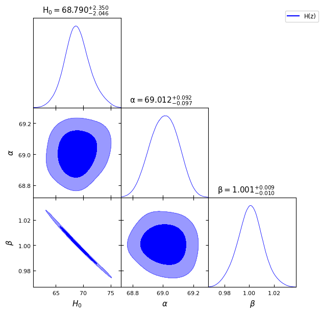
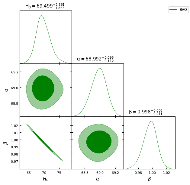
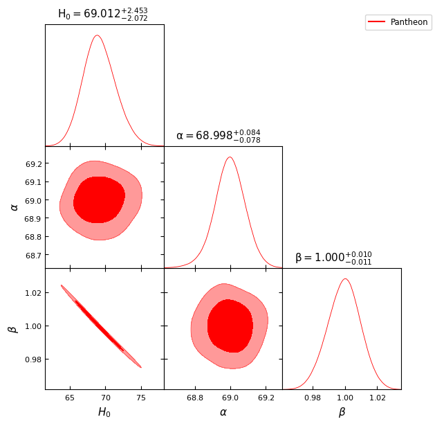
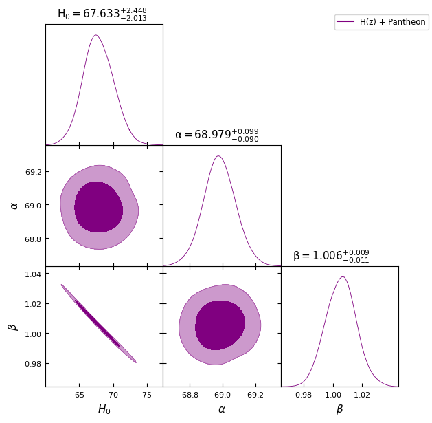
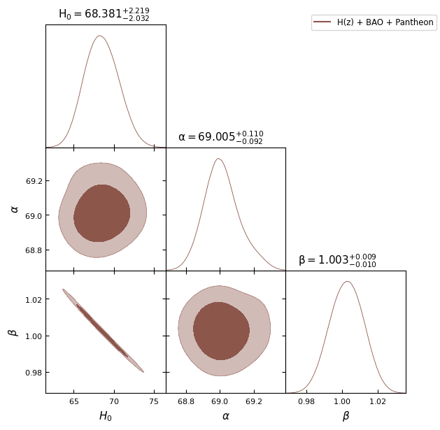
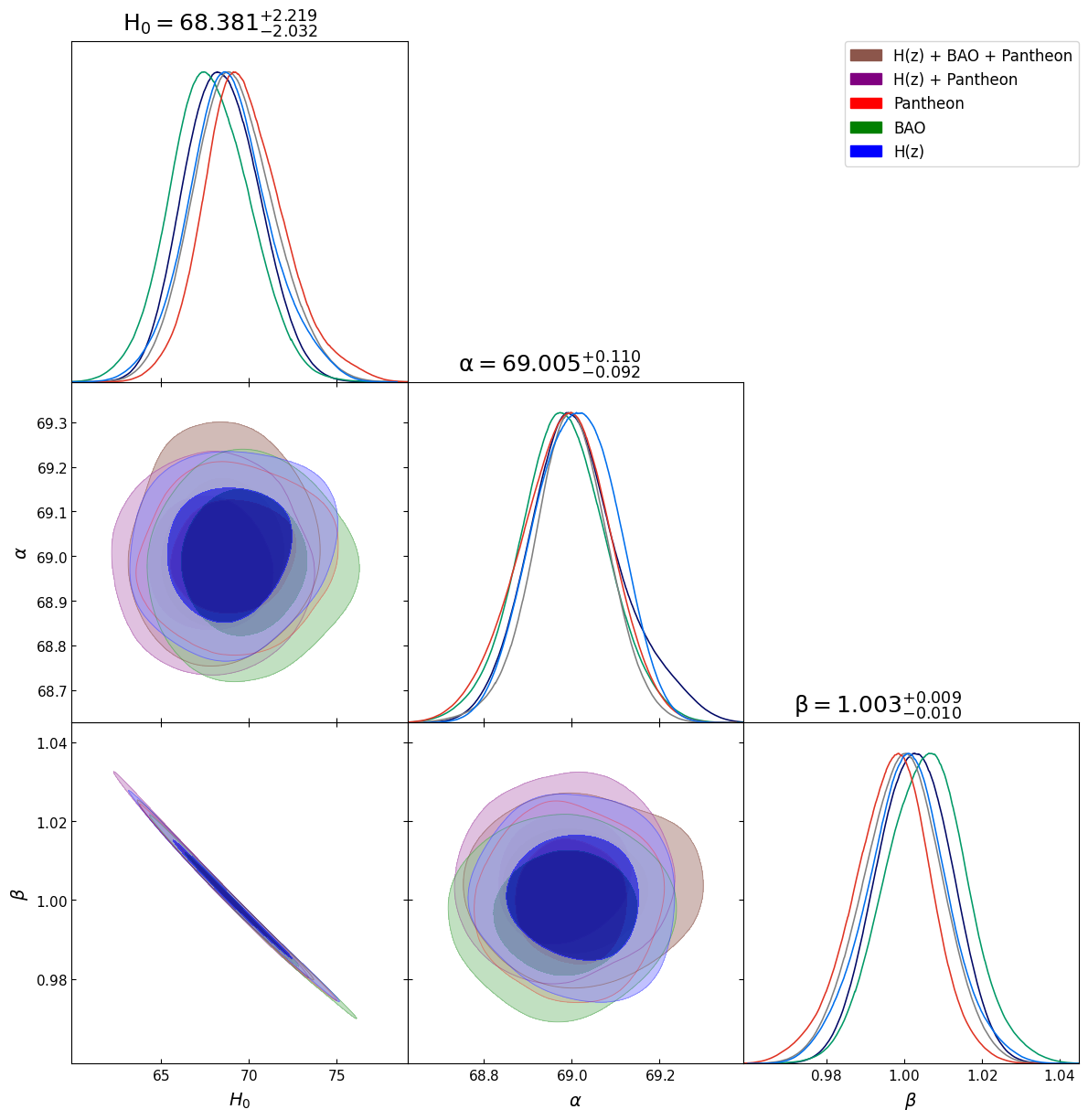
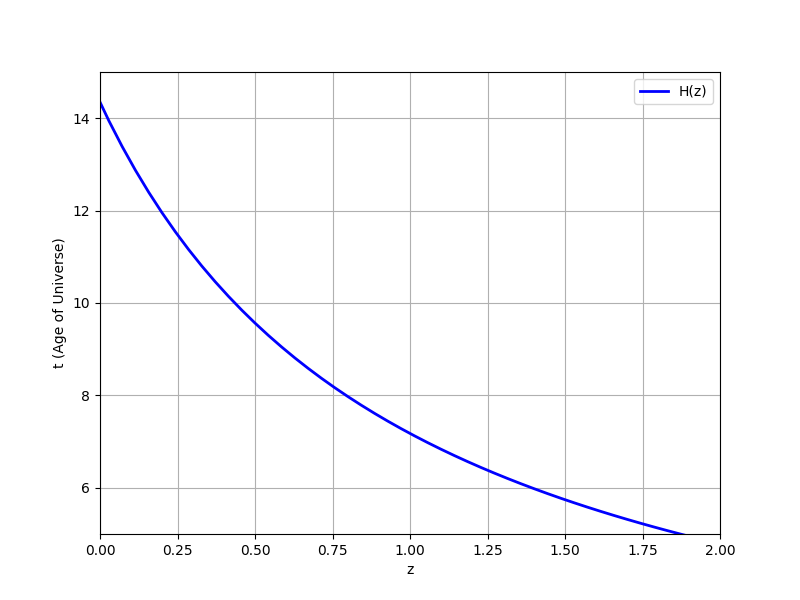
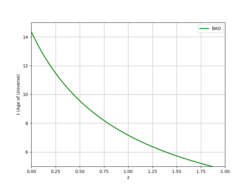
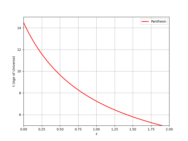
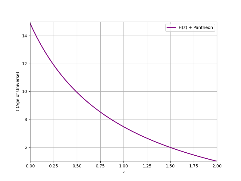
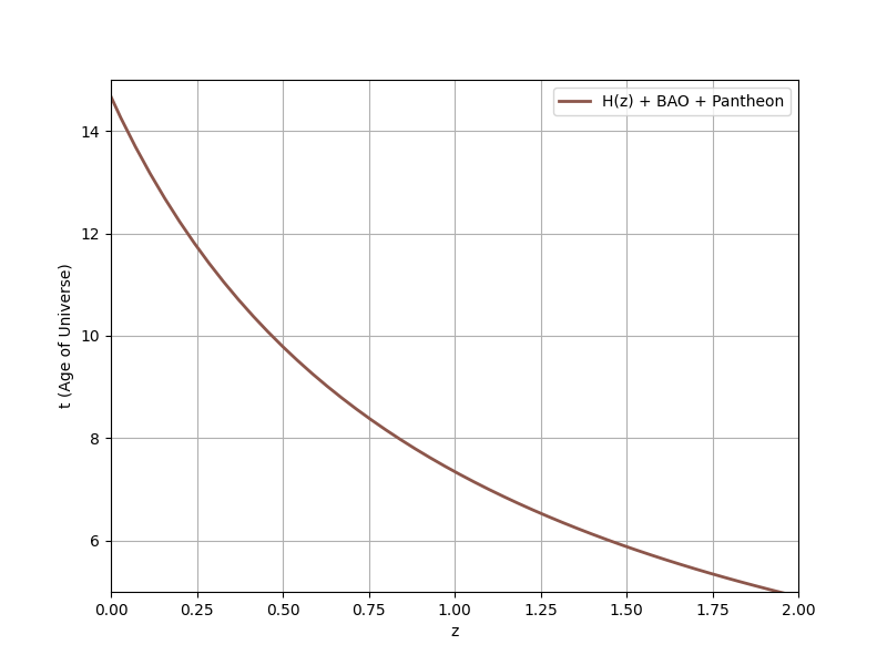
Figures 1 6 depict marginalized distribution and contour diagrams for the derived model and the estimated value of the parameters extracted from OHD, BAO, Pantheon compilation of SN Ia and joined datasets respectively. The parametric values (viz. , , and the age of Universe in Gyr ) obtained from different datasets due to MCMC and Bayesian analysis are tabulated in Table 1. The graphical representation of cosmic age over redshift in exhibited in Fig. 7. Five plots are for different combinations of , BAO, Pantheon datasets and their combinations. The Age of universe at is mentioned in Table 1.
| Parameter | H(z) | BAO | Pantheon | ||
|---|---|---|---|---|---|
4 Energy conditions and cosmological Parameters
4.1 Energy Conditions
The energy conditions analogously establish cosmic laws that elucidate the distribution of matter and energy throughout the cosmos, which can be derived from Einstein’s gravitational equations. Thus, we obtain certain conditions, viz. Weak Energy Condition (WEC), Null Energy Condition (NEC), Strong Energy Condition (SEC), and Dominant Energy Condition (DEC) reveal the distribution of matter and energy in the cosmic space.
-
1.
WEC:
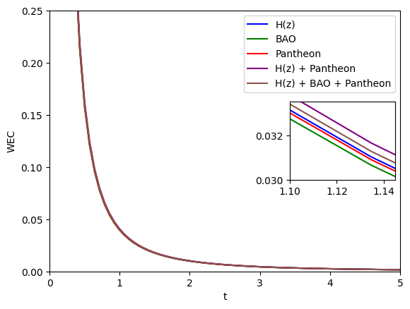
According to the WEC, energy cannot be negative or zero. This requirement keeps the laws of the cosmos impartial and constant. Using the parameters discovered using the Bayesian Analysis, Fig. 14 depicts the WEC’s nature for our model. -
2.
NEC:
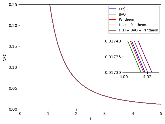
The NEC deals with light. It asserts that energy is a necessary component of all space transit for light and cannot exist in a vacuum. This constraint prevents odd occurrences from occurring and maintains the physics of the cosmos. Figure 11 illustrates the characteristics of NEC for our model utilizing the Bayesian Analysis’s parameters. -
3.
SEC:
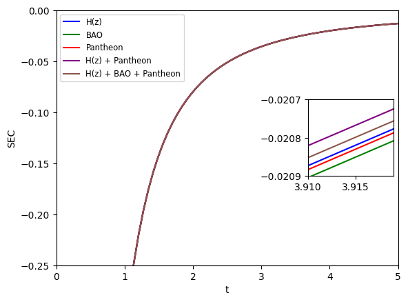
Similar to a more rigid counterpart of the NEC, the SEC guarantees that the energy cannot be negative and sets a boundary for how objects respond to gravity. The cosmos benefits from having this rule in place. Figure 13 depicts the characteristics of SEC for our model utilizing the Bayesian analysis. -
4.
DEC:
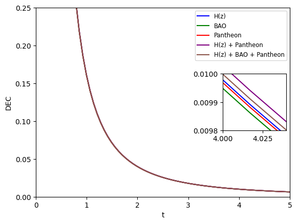
The DEC guarantees that the energy is not just non-negative but also that its distribution cannot be too volatile. It is comparable to asserting that energy cannot go out of control or travel faster than light. Based on the Bayesian Analysis, DEC is shown in Fig. 12.
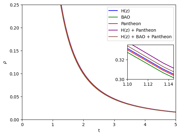
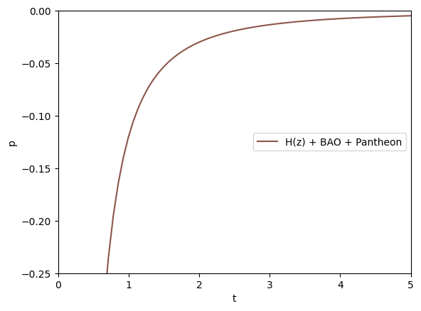
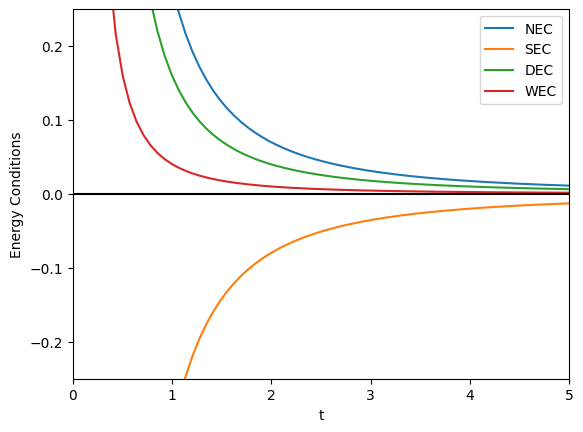
All the above-mentioned energy conditions combined are as shown in Fig. 15. Figure 8 displays the distribution of energy density wrt time , while Fig. 9 displays the distribution of pressure. Our results demonstrate that, except for SEC the others, e.g., NEC, WEC and DEC are fulfilled. The late-rapid expansion of the universe justifies the violation of SEC. The theory of gravity, having a contribution from the trace energy can suitably explain the late-time accelerated phase of the universe without invoking any need for the cosmological constant or exotic dark energy as the background agent for the phenomenon.
4.2 State Finder Diagnotics
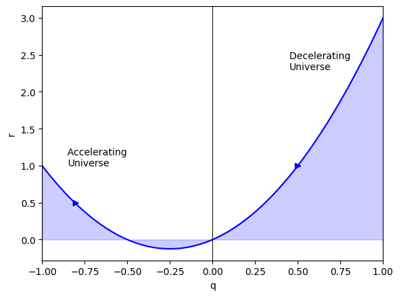
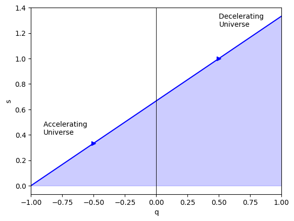
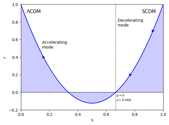
The state finder diagnostics are a kind of pathological testings which can assist to find out the puzzles of dark energy and thus the history of the cosmos. These diagnostics are based on the and parameters and we can comprehend the evolution of the cosmos by using these factors in a better way as that provide information on the expansion of the universe and the elements that make it up. These dimensionless parameters help us understand the fundamental dynamics of the cosmos having definitions as follows:
| (20) |
| (21) |
The above two equations for the model under consideration take the following forms:
| (22) |
| (23) |
The scale factor trajectories in the resulting model may be shown in Fig. 16 to follow a specific set of paths. Interestingly, our strategy is consistent with the results for the cosmic diagnostic pair from power law cosmology.
4.3 Om(z) parameter
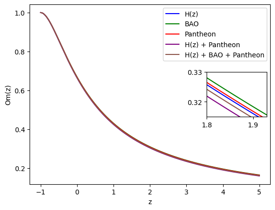
The state finder parameters and the diagnostic are usually applied to analyse various dark energy ideas. Basically, the parameter is deployed when the Hubble parameter and the cosmic redshift merge in a suitable way. The parameter in the alternative gravity is read as
| (24) |
The Hubble parameter is shown by in this case. Shahalam et al. [38] claim that the negative, zero and positive values of , respectively, represent the quintessence (), -CDM and phantom () dark energy theories. However, for the present model, we obtain this parameter as follows:
| (25) |
4.4 Jerk Parameter
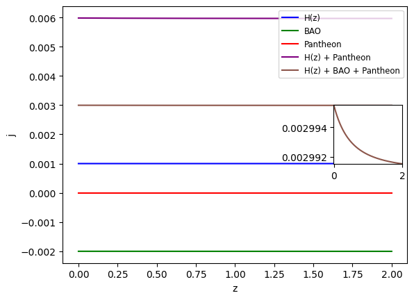
After the Hubble and deceleration parameters, the jerk parameter is one that can provide deeper insights into the universe’s history. The universe’s acceleration is tracked throughout time by the jerk parameter, indicated by the symbol . The acceleration is accelerating and speeding up phase when is positive (), whereas the acceleration is said to slow down if is negative (). However, different dark energy theories forecast various jerk parameter values, and thus, scientists can learn more about dark energy by measuring and comparing it to these predictions. The jerk parameter contributes to the improvement of our models of the cosmos when paired with other cosmic factors. It puts these models to a rigorous examination to ensure they truly reflect what we observe in the physical cosmos. In this context, we note that Fig. 18 depicts the fluctuation of with respect to redshift for our model and the derived parameters.
.
5 Conclusion
In the present work our aim was to find the possibility of a Bianchi V type Universe under gravity theory. For this purpose we have proposed for a viable Lagrangian model based on the connection between the trace of the energy-momentum tensor and the Ricci scalar . However, in order to solve the related field equations we have considered a power law for the scaling factor.
The investigation provides the following salient features:
(i) To compare the model parameters with the observational data we impose constraint on the model using the datasets from the Hubble parameter , BAO, Pantheon, combined + Pantheon, and combined + BAO + Pantheon. The outcomes for under our gravity model are as follows: km s-1 Mpc-1, km s-1 Mpc-1, km s-1 Mpc-1, km s-1 Mpc-1, km s-1 Mpc-1, respectively.
(ii) Our estimation of is remarkably consistent with various recent Planck Collaboration studies that utilize the -CDM model.
(iii) We have addressed the energy conditions, analysis and cosmographical parameters which are equivocally very responsive and informative for physical viability of our model.
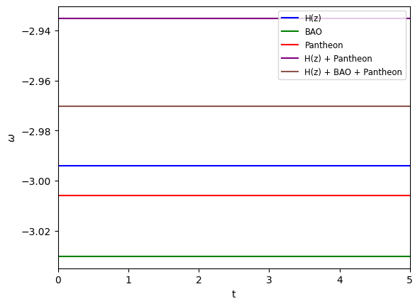
(iv) Graphical presentations of different model parameters are shown in several figures which are very informative in their nature. Among all these the Fig. 10, considering the relationship between the state parameter of the equation and the passage of time implies that dark energy plays a role in the accelerated expansion of the universe, while its exact nature varies over time. This finding could have intriguing cosmological implications.
Overall observation and conclusion can be put forward as follows: the obtained results demonstrate that the proposed model mostly agrees with the observational signatures of the cosmological scenario within a certain range of restrictions.
Data Availability
This research did not yield any new data..
Conflict of Interest
The authors declare no conflict of interest.
Acknowledgement
SR would like to express his gratitude to the ICARD facilities at CCASS, GLA University, Mathura, as well as the Visiting Research Associateship Programme at the Inter-University Centre for Astronomy and Astrophysics (IUCAA) in Pune, India.
References
- [1] A. G. Riess et al. [Supernova Search Team], Observational evidence from supernovae for an accelerating universe and a cosmological constant, Astron. J. 116, 1009-1038 (1998)
- [2] A. G. Riess et al. [Supernova Search Team], Type Ia supernova discoveries at z 1 from the Hubble Space Telescope: Evidence for past deceleration and constraints on dark energy evolution, Astrophys. J. 607, 665-687 (2004)
- [3] M. Tegmark et al. [SDSS], Cosmological parameters from SDSS and WMAP, Phys. Rev. D 69, 103501 (2004)
- [4] E. Calabrese, M. Migliaccio, L. Pagano, G. De Troia, A. Melchiorri and P. Natoli, Cosmological constraints on the matter equation of state, Phys. Rev. D 80, 063539 (2009)
- [5] Y. Wang and M. Dai, Exploring uncertainties in dark energy constraints using current observational data with Planck 2015 distance priors, Phys. Rev. D 94, no.8, 083521 (2016)
- [6] M. M. Zhao, D. Z. He, J. F. Zhang and X. Zhang, Search for sterile neutrinos in holographic dark energy cosmology: Reconciling Planck observation with the local measurement of the Hubble constant, Phys. Rev. D 96, no.4, 043520 (2017)
- [7] B. Wang, E. Abdalla, F. Atrio-Barandela and D. Pavon, Dark Matter and Dark Energy Interactions: Theoretical Challenges, Cosmological Implications and Observational Signatures, Rept. Prog. Phys. 79, 096901 (2016)
- [8] P. J. E. Peebles and B. Ratra, The Cosmological Constant and Dark Energy, Rev. Mod. Phys. 75, 559-606 (2003)
- [9] T. Padmanabhan, Cosmological constant: The Weight of the vacuum, Phys. Rept. 380, 235-320 (2003)
- [10] E. Abdalla and A. Marins, The Dark Sector Cosmology, Int. J. Mod. Phys. D 29, 2030014 (2020)
- [11] M. Li, X. D. Li, S. Wang and Y. Wang, Dark Energy: A Brief Review, Front. Phys. (Beijing) 8, 828-846 (2013)
- [12] V. Sahni, The Cosmological constant problem and quintessence, Class. Quant. Grav. 19, 3435-3448 (2002)
- [13] J. Garriga and A. Vilenkin, Solutions to the cosmological constant problems, Phys. Rev. D 64, 023517 (2001)
- [14] J. Frieman, M. Turner and D. Huterer, Dark Energy and the Accelerating Universe, Ann. Rev. Astron. Astrophys. 46, 385-432 (2008)
- [15] S. Nojiri and S. D. Odintsov, Unified cosmic history in modified gravity: from theory to Lorentz non-invariant models, Phys. Rept. 505, 59-144 (2011)
- [16] L. Samushia and B. Ratra, Constraining dark energy with gamma-ray bursts, Astrophys. J. 714, 1347-1354 (2010)
- [17] M. Yashar, B. Bozek, A. Abrahamse, A. Albrecht and M. Barnard, Exploring Parameter Constraints on Quintessential Dark Energy: the Inverse Power Law Model, Phys. Rev. D 79, 103004 (2009)
- [18] Harko, Tiberiu, Francisco SN Lobo, Shin’ichi Nojiri, and Sergei D. Odintsov, gravity, Phys. Rev. D 84, 024020 (2011)
- [19] T. Harko, Thermodynamic interpretation of the generalized gravity models with geometry - matter coupling, Phys. Rev. D 90, no.4, 044067 (2014)
- [20] L. K. Sharma, A. K. Yadav, P. K. Sahoo and B. K. Singh, Non-minimal matter-geometry coupling in Bianchi I space-time, Res. Phys. 10, 738-742 (2018)
- [21] A. K. Yadav, L. K. Sharma, B. K. Singh and P. K. Sahoo, Existence of bulk viscous universe in gravity and confrontation with observational data, New Astron. 78, 101382 (2020)
- [22] L. K. Sharma, A. K. Yadav and B. K. Singh, Power-law solution for homogeneous and isotropic universe in gravity, New Astron. 79, 101396 (2020)
- [23] L. K. Sharma, B. K. Singh and A. K. Yadav, Viability of Bianchi type V universe in gravity, Int. J. Geom. Meth. Mod. Phys. 17, 2050111 (2020)
- [24] S. Nojiri and S. D. Odintsov, Unified cosmic history in modified gravity: from theory to Lorentz non-invariant models, Phys. Rept. 505, 59-144 (2011)
- [25] S. M. Carroll, V. Duvvuri, M. Trodden and M. S. Turner, Is cosmic speed-up due to new gravitational physics? Phys. Rev. D 70, 043528 (2004)
- [26] W. Hu and I. Sawicki, Models of Cosmic Acceleration that Evade Solar-System Tests, Phys. Rev. D 76, 064004 (2007)
- [27] F. G. Alvarenga, A. de la Cruz-Dombriz, M. J. S. Houndjo, M. E. Rodrigues and D. Sáez-Gómez, Dynamics of scalar perturbations in gravity, Phys. Rev. D 87, 103526 (2013)
- [28] P. K. Sahoo, P. Sahoo and B. K. Bishi, Anisotropic cosmological models in gravity with variable deceleration parameter, Int. J. Geom. Meth. Mod. Phys. 14, 1750097 (2017)
- [29] Z. Yousaf, K. Bamba and M. Z. u. H. Bhatti, Causes of Irregular Energy Density in Gravity, Phys. Rev. D 93, 124048 (2016)
- [30] Z. Yousaf, M. Z. u. H. Bhatti and M. Ilyas, Existence of compact structures in gravity, Eur. Phys. J. C 78, 307 (2018)
- [31] Z. Yousaf, K. Bamba and M. Z. u. H. Bhatti, Influence of Modification of Gravity on the Dynamics of Radiating Spherical Fluids, Phys. Rev. D 93, 064059 (2016)
- [32] Z. Yousaf, K. Bamba, M. Z. Bhatti and U. Ghafoor, Charged Gravastars in Modified Gravity, Phys. Rev. D 100, 024062 (2019)
- [33] A. Das, F. Rahaman, B. K. Guha and S. Ray, Compact stars in gravity, Eur. Phys. J. C 76, 654 (2016)
- [34] A. K. Yadav, P. K. Sahoo and V. Bhardwaj, Bulk viscous Bianchi-I embedded cosmological model in gravity, Mod. Phys. Lett. A 34, 1950145 (2019)
- [35] S. V. Lohakare, B. Mishra, S. K. Maurya, Ksh. N. Singh, Analyzing the Geometrical and Dynamical Parameters of Modified Teleparallel- Gauss-Bonnet Model, arXiv: 2209.13197.
- [36] S. Alam et al. (eBOSS), Completed SDSS-IV extended Baryon Oscillation Spectroscopic Survey: Cosmological implications from two decades of spectroscopic surveys at the Apache Point Observatory, Phys. Rev. D 103, 083533 (2021).
- [37] D. M. Scolnic et al., The Complete Light-curve Sample of Spectroscopically Confirmed SNe Ia from Pan-STARRS1 and Cosmological Constraints from the Combined Pantheon Sample, Astrophys. J. 859, 101 (2018).
- [38] M. Shahalam, S. Sami and A. Agarwa, Mon. Not. R. Astron. Soc. 448, 2948 (2015).