Period-Luminosity-Metallicity-Color Relations of Late-type Contact Binaries in the Big Data Era

Abstract

Binary stars ubiquitous throughout the universe are important. Contact binaries (CBs) possessing Period-Luminosity (PL) relations could be adopted as distance tracers. The PL relations of CBs are influenced by metallicity abundance and color index, which are connected to both the radius and luminosity of stars. Here we propose fine relations of Period-Luminosity-Metallicity-Color (PLZC) from the ultraviolet to infrared bands based on current surveys. The accuracy of the distance estimation is 6% and 8%, respectively, depending on the PLZC relations of the CBs in the infrared and optical bands of the collected data. PLZC models are still more accurate than PLC models in determining intrinsic luminosity, notwithstanding their limited improvement. Meanwhile, these relations based on synthetic photometry are also calibrated. On the basis of the synthetic photometry, a 6% accuracy of distance is estimated. The measured or synthetic data of PLZC or PLC relations in infrared bands comes first in the list of suggestions for distance estimations, and is followed by the measured data of optical bands.

1 Introduction

In the Milky Way, more than half of stars belong to binary systems, which are important to study in many fields, such as stellar physics (Arcones & Thielemann, 2023), Galaxy and extra-galaxies (Kormendy et al., 2009), cosmology (Pietrzyński et al., 2013), and gravitational wave astronomy (Abbott et al., 2017). When the host star is filled with Roche critical volume, the process of material exchange begins accompany with the essence of energy exchange. Therefore, material and energy exchanges are inseparable physical processes, which provide conditions for the formation of some special stars, such as red novae (Tylenda et al., 2011; Matsumoto & Metzger, 2022), type Ia supernovae (Webbink, 1984; Iben & Tutukov, 1984; Whelan & Iben, 1973), short gamma-ray bursts (Shibata & Taniguchi, 2006; Fong & Berger, 2013), binary black hole mergers (Abbott et al., 2016), and kilonovae (Smartt et al., 2017; Cowperthwaite et al., 2017).

These binary systems with significant material exchange between the primary and its companion star are called close binary stars, which are common among binary systems. According to the overall evolution, close binary stars are divided into three types: detached, semi-detached, and contact phases. Contact binary stars (CBs) with two companions full of their own Roche lobes share a common external envelope. Then tidal interactions make them rotate rapidly and produce magnetic activities similar to the Sun (Devarapalli et al., 2020; Kang et al., 2004; Jeong & Kim, 2011). Generally, binary systems with common envelope will lose the shell through the outer Lagrange point, thus becoming a system with very short orbital period. Most importantly, CBs can be used as distance indicators based on Period-Luminosity relation (Ruciński, 1994).

Since CBs proposed as distance tracers by Eggen (1967), various studies have tried to establish Period-Luminosity (PL) and Period-Luminosity-Color (PLC) relations of CBs. This issue has also attracted attention and research of Ruciński (1974). Mochnacki (1981) derived the PL relation based on a sample of 37 CBs, but the work mainly focuses on the mass-brightness relation. Because the effective temperature and luminosity are interrelated, it is necessary to consider the color index term for calibrating the absolute magnitude. Ruciński (1994) calibrated the absolute magnitude based on $B$, $V$, and $I$-band of CBs in open clusters, established the first accurate PLC relations. The relations are re-calibrated based on 40 CBs with Hipparcos parallax (Ruciński & Duerbeck, 1997). Then, Eker et al. (2009) analyzed 31 CBs with the most accurate distance by applying Lutz-Kelker corrections (Lutz & Kelker, 1973) to the parallax from the Hipparcos catalog, and re-calibrated the classic PLC relation of Ruciński & Duerbeck (1997). Meanwhile, they extended the PLC relations to the near-infrared $J$, $H$, and $K_{s}$-band. Independently, Chen et al. (2016) calibrated the distances of a sample of 66 CBs from open clusters based on Hipparcos parallaxes to derived near-infrared $J$, $H$, and $K_{s}$-band PL relations. Furthermore, Chen et al. (2018) established PL relations for 12 bands from optical to mid-infrared bands based on 183 nearby CBs (within 300 pc) with accurate Tycho-Gaia parallax (Gaia Collaboration et al., 2016), obtaining that the minimum scatter of absolute magnitude is 0.16 mag. For the first time, PL and PLC relations for late-type CBs are established by Ngeow et al. (2021) based on $g$, $r$, and $i$-band light curves collected by Zwicky Transient Factory (ZTF, Graham et al., 2019).

In earlier work of Ruciński (1995, 2000), they discussed that metallicity may have an impact on the PL relation. The PL relation were more susceptible to redness correction uncertainties, so it was not necessary to retain the metallicity term in the PL relation (Ruciński, 2004). However, CBs will become brighter about 0.2 mag in the near-infrared bands when the metallicity ($[\rm Fe/H]$) decreases by 1 dex (Chen et al., 2016). Benefited from the coverage and precision of current surveys, more accurate PL relations for CBs in a large sample of all sky could be established.

In this work, we makes comparisons between PL, Period-Luminosity-Metallicity (PLZ), PLC, and Period-Luminosity-Metallicity-Color (PLZC) relations based on currently surveys. The dispersion of PLZC relation is minimal for ultraviolet to infrared bands. In Sect. 2, we describe the data of CBs adopted in this work. In Sect. 3, the fitting models and results are presented, followed by discussions and conclusions in Sect. 4.

2 Data

With the increase of high-cadence, long-term, and high-precision photometric surveys in recent years, more and more CBs have been identified, which construct a large sample to carry out various of researches. The data of CBs analyzed in this work are collected based on the General Catalogue of Variable Stars (Version GCVS 5.1, Samus’ et al., 2017), the All-Sky Automated Survey for Supernovae (ASAS-SN, Jayasinghe et al., 2019), and the Northern Catalina Sky Survey (CSS, Sun et al., 2020). The latest released data from those catalogues contains 3261, 76378, and 2335 CBs, respectively.

The photometric data analyzed in this work covers the bands of Gaia DR3 (Gaia Collaboration, 2022), WISE (Cutri et al., 2021) and GALEX (Bianchi et al., 2017). The distances (parallaxes) of the CBs are adopted from Gaia DR3. The LAMOST spectroscopic survey provides the largest database of low and median-resolution spectra to measure stellar atmospheric parameters and radial velocities for millions of stars (Cui et al., 2012; Zhao et al., 2012; Deng et al., 2012; Liu et al., 2014; Yuan et al., 2015). Metallicity abundance ($[\rm Fe/H]$) and effective temperature ($T_{\rm eff}$) of the CBs are obtained through cross-matching with the catalogs of LAMOST Data Release 9, which are derived through the LAMOST stellar parameter pipeline (LASP, Luo et al., 2015). In total, 6883 unique CBs are selected with complete information such as photometric, astrometric, and spectroscopic parameters. A summary of the CBs is shown in Table 1. The duplicate data has been removed to optimize redundancy, and the total number of duplicates is shown in parentheses.

Table 1: CBs collected from different surveys or catalogs.

Surveys	Number of CBs	LAMOST DR9	Gaia DR3	WISE	GALEX
GCVS	3,261	680	655	652	368
ASAS-SN	76,378	6,503	6,221	6,110	2,447
CSS	2,335	720	704	694	359
Total	81,974	7,903	6,883(697)	6,772(685)	2,844(330)

Based on the different distributions of orbital periods and spectral characteristics between early and late-type CBs, late-type ones are selected by using a period-temperature relation or a period cut. We apply the both methods to limit the sample to avoid mixing early and late-type CBs as much as possible. Figure 1 presents the $T_{\rm eff}$ versus $\log P$ of the CBs. The solid and dashed lines present the thresholds, $T_{\rm eff}=6710\ \rm K-1760\ K\log(P/0.5\ day)$ and $\log P=-0.30$ day given in Jayasinghe et al. (2020), respectively. After applying the thresholds, the black squares are classified into late-type CBs, while the gray triangles are considered to be the early-type ones.

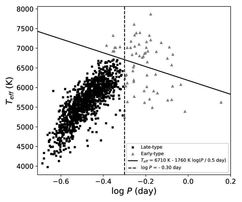
Figure 1: $\rm T_{eff}$ versus $\log P$ for CBs in our sample. Black squares denote the late-type CBs, while gray triangles early-type ones.

For the remaining late-type CBs, to make sure the reliability of the following calibrations, we exclude the inaccurate distance measurement data with $\tt Parallax\_over\_error$ less than 80. We also exclude some sources with large absolute magnitude errors, such as Gaia $G$, $B_{p}$, and $R_{p}$-band, whose absolute magnitude errors are larger than 0.04, 0.07, and 0.07 mag, respectively. Therefore, the final sample of CBs for calibrations are listed in Table 2, which could be download online.

Table 2: The final sample of CBs for calibrations.

Clo.	Name	Units	Description	Example
1	Gaia_source_id	—	Gaia SOURCE_ID	1038711452258591744	…
2	RA	deg	Degree of Right Ascension (J2000)	142.236	…
3	Dec	deg	Degree of Declination (J2000)	59.935	…
4	Parallax	mas	Gaia DR3 parallax	5.599	…
5	Parallax_over_error	—	Parallax divided by its standard error	450.226	…
6	Period	day	Orbital period	0.2488	…
7	$T_{\rm eff}$	K	Effective temperature from LAMOST	4851	…
8	$T_{\rm eff}$_err	K	Effective temperature error	32	…
9	[Fe/H]	dex	[Fe/H] from LAMOST	-0.067	…
10	[Fe/H]_err	dex	[Fe/H] error	0.027	…
11	$\langle FUV\rangle$	mag	GALEX FUV_band mean magnitude	21.806	…
12	FUV_err	mag	Error on FUV_band mean magnitude	0.231	…
13	$\langle NUV\rangle$	mag	GALEX NUV_band mean magnitude	18.973	…
14	NUV_err	mag	Error on NUV_band mean magnitude	0.023	…
15	$\langle Bp\rangle$	mag	Gaia DR3 Bp_band mean magnitude	12.537	…
16	Bp_err	mag	Error on Bp_band mean magnitude	0.010	…
17	$\langle G\rangle$	mag	Gaia DR3 G_band mean magnitude	12.025	…
18	G_err	mag	Error on G_band mean magnitude	0.004	…
19	$\langle Rp\rangle$	mag	Gaia DR3 Rp_band mean magnitude	11.336	…
20	Rp_err	mag	Error on Rp_band mean magnitude	0.008	…
21	$\langle W1\rangle$	mag	WISE W1_band mean magnitude	9.799	…
22	W1_err	mag	Error on W1_band mean magnitude	0.022	…
23	$\langle W2\rangle$	mag	WISE W2_band mean magnitude	9.831	…
24	W2_err	mag	Error on W2_band mean magnitude	0.02	…
25	$\langle W3\rangle$	mag	WISE W3_band mean magnitude	9.787	…
26	W3_err	mag	Error on W3_band mean magnitude	0.034	…
27	$\langle W4\rangle$	mag	WISE W4_band mean magnitude	8.846	…
28	W4_err	mag	Error on W4_band mean magnitude	0.331	…

Note. — The Table is published in its entirety in the machine-readable format. A portion is shown here for guidance regarding its form and content.

The extinction is estimated through the full-sky 3D dust-reddening map of $E(B-V)$ based on the dust thermal emission generated by Green et al. (2019). A value of 3.1 for $R_{\rm v}$ is adopted to estimate the extinction by applying the equation $A_{\rm v}=R_{\rm v}E(B-V)$. Additionally, extinction values in other bands are estimated based on the relative extinction values $A_{\lambda}/A_{\rm v}$ from Jordi et al. (2010), Wang et al. (2018), Wang & Chen (2019), and Rieke & Lebofsky (1985). The absolute magnitudes of the sample are deduced through the following equation,

$$M=m-5\log D+5-A_{\rm\lambda},$$ (1)

where $M$ and $m$ are absolute and apparent magnitudes, respectively. The quantity $D$ denotes the distance from Gaia astrometry, and $A_{\rm\lambda}$ is extinction described previously.

The left panel of Fig. 2 shows the locations of the CBs shift with periods in color-magnitude diagram (CMD). It demonstrates that the luminosity of late-type CBs are related to periods as well as stellar colors (e.g. $B_{p}-R_{p}$ color index from Gaia). Meanwhile, the right panel of the figure presents that metallicity-poor stars are bluer than metallicity-rich ones, which demonstrates the influences of metallicity on the positions of CBs in CMD. Therefore, the positions of CBs on CMD are related both to the period and $[\rm Fe/H]$, which confirms the influences of metallicity and color index on PL relations.

Figure 2: CBs distribution on CMD. G and $B_{p}-R_{p}$ denote the extinction corrected absolute magnitude and color index, respectively. The colorbars in left and right panels denote Period ($\log P$) and metallicity abundance ($[\rm Fe/H]$), respectively.

3 Calibration of PL relations for late-type CBs

The PLZC relations are derived with the periods, mean magnitude, metallicity abundance and color index of $B_{p}-R_{p}$ described in Sect. 2. As comparisons, the PL, PLZ, and PLC relations are derived simultaneously. These relations are calibrated by fitting the following equations,

$$M=a\log P+b,$$ (2)

$$M=a\log P+b+c[\rm Fe/H],$$ (3)

$$M=a\log P+b+d(B_{p}-R_{p}),$$ (4)

$$M=a\log P+b+c{\rm[Fe/H]}+d(B_{p}-R_{p}),$$ (5)

where $a$, $b$, $c$, and $d$ are set as free parameters to fit. To obtain the best-fitting relations, we refer to a Python implementation, emcee, of Markov Chain Monte Carlo (MCMC) proposed by Goodman & Weare (2010).

3.1 PLZC and other relations for measured data

The PL relations for each band are calibrated firstly. The fitting performances of the PL relations from ultraviolet to infrared bands are shown as corner plots in Fig. 3. These corner plots show that the PL models are well fitted. The coefficients and their errors of the best-fitting relations are texted at the tops of the panels. The numbers used for determining these relations are in the second column of Table 3. Their slopes and intercepts are listed in the third and fourth columns. To quantify the differences between absolute magnitudes from observations and these from models, a quantity $\delta$ is defined as,

$$\delta=M_{obs}-M_{model},$$ (6)

where $M_{obs}$ denote the absolute magnitude directly from observations, while $M_{model}$ is the absolute magnitude deduced through equations 2 - 5 based on period and other observed quantities. Then, the dispersion, $\sigma$, of the calibrated relations are derived by fitting the $\delta$ distribution with a Gaussian profile. The Gaussian-fitted distribution of $\delta$ are shown in Fig. 4, represented by a red dotted line. The figure shows that the dispersion of PL relations in the FUV, NUV, and W4 bands is large. The large dispersion may be due to significant photometric errors and limited sample size (Zhang & Yuan, 2023).

Figure 3: Parameters fitting for PL relations by emcee in each band, and tops of the panels are the best parameters obtained by fitting.

Table 3: Parameters of PL models for multi-band.

Band	Number	a	b	$\sigma$ (mag)
$FUV$	199	$-$11.03($\pm 0.3$)	8.40($\pm 0.13$)	1.17
$NUV$	632	$-$13.17($\pm 0.03$)	3.05($\pm 0.01$)	1.45
$B_{p}$	1,093	$-$10.11($\pm 0.01$)	$-$0.10($\pm 0.01$)	0.45
$G$	1,093	$-$9.34($\pm 0.01$)	$-$0.10($\pm 0.01$)	0.37
$R_{p}$	1,093	$-$8.33($\pm 0.01$)	$-$0.20($\pm 0.01$)	0.33
$W1$	1,019	$-$6.01($\pm 0.20$)	$-$0.16($\pm 0.01$)	0.16
$W2$	1,019	$-$6.03($\pm 0.20$)	$-$0.14($\pm 0.01$)	0.17
$W3$	992	$-$5.86($\pm 0.04$)	$-$0.14($\pm 0.02$)	0.24
$W4$	127	$-$1.71($\pm 0.19$)	$-$0.38($\pm 0.01$)	1.21

Note. — The parameters a and b are the best-fitting coefficients in equation 2, and $\sigma$ are the dispersion of PL relations.

Figure 4: Distributions of $\delta$ for each bands. The fitted Gaussian function to the histogram is shown as dash line.

To verify the influence of metallicitiy abundance on PL relations, PLZ relations from ultraviolet to infrared bands are aslo derived. Corner plots of emcee fitting of equation 3 are presented in Fig. 5. Table 4 summarizes their fitting parameters and responding dispersion. The dispersions are improved when considering the influence of [Fe/H] on PL relations. With 1.0 dex increasing of $\rm[Fe/H]$, the CBs will be dimmer of 0.28 - 2.86 mag for the ultraviolet to infrared bands. It is slightly higher than 0.2 mag proposed by Chen et al. (2016). To present the fitting results of the PLZ relations on $\rm Period$-$\rm Magnitude$ diagram, we choose three values, -1.0, -0.2, and 0.5 dex of $\rm[Fe/H]$, as examples in Fig. 6. It sees from the figure that the PLZ relations fit the observations better than hte PL relations.

Figure 5: Parameters fitting for PLZ relations by emcee.

Table 4: Parameters of PLZ models for multi-band.

Band	Number	a	b	c	$\sigma$ (mag)
$FUV$	199	$-$12.96($\pm 0.32$)	7.75($\pm 0.13$)	2.16($\pm 0.08$)	0.71
$NUV$	632	$-$17.57($\pm 0.02$)	1.36($\pm 0.02$)	2.86($\pm 0.01$)	0.82
$B_{p}$	1,093	$-$11.50($\pm 0.02$)	$-$0.79($\pm 0.01$)	0.97($\pm 0.01$)	0.28
$G$	1,093	$-$10.54($\pm 0.02$)	$-$0.71($\pm 0.01$)	0.82($\pm 0.01$)	0.25
$R_{p}$	1,093	$-$9.46($\pm 0.02$)	$-$0.76($\pm 0.01$)	0.67($\pm 0.01$)	0.22
$W1$	1,019	$-$6.37($\pm 0.02$)	$-$0.34($\pm 0.01$)	0.28($\pm 0.01$)	0.12
$W2$	1,019	$-$6.43($\pm 0.02$)	$-$0.34($\pm 0.01$)	0.31($\pm 0.01$)	0.14
$W3$	992	$-$6.20($\pm 0.04$)	$-$0.30($\pm 0.02$)	0.31($\pm 0.01$)	0.22
$W4$	127	$-$2.92($\pm 0.20$)	$-$0.90($\pm 0.09$)	1.28($\pm 0.07$)	1.40

Note. — The parameters a, b, and c are best-fitting coefficients in equation 3, and $\sigma$ denote the deviations of PLZ relations.

Figure 6: The $\rm Period$-$\rm Magnitude$ diagram. The colorbar presents the value of $[\rm Fe/H]$. The dotted-lines in each panel present examples of PLZ relation with given $\rm[Fe/H]$, while the solid lines present the best-fitting PL relations.

According to Roche-lobe theory (Eggleton, 1983), it is anticipated that the correlation between the CBs orbital period and absolute magnitudes will include both the effective temperature of the system and the color term. The PLC relations for multi bands by using equation 4 are calibrated, of which the performance are shown in Fig. 7. Table 5 summarizes their fitting parameters and dispersion. Similarly, we also show the result of PLC relations on Fig. 8. The slope of $\log P$ in the PLC relations are lower in comparison to the PL and PLZ relations, which proves the contribution of color term to calibrations. The figure shows that the magnitudes of CBs are more sensitive to color term than metallicitiy term.

Figure 7: Parameters fitting for PLC relations by emcee.

Table 5: Parameters of PLC models for multi-band.

Band	Number	a	b	d	$\sigma$ (mag)
$FUV$	199	$-$5.67($\pm 0.36$)	7.24($\pm 0.13$)	4.29($\pm 0.15$)	0.61
$NUV$	632	$-$3.74($\pm 0.03$)	0.58($\pm 0.01$)	7.94($\pm 0.02$)	0.36
$B_{p}$	1,093	$-$4.26($\pm 0.02$)	$-$0.50($\pm 0.01$)	3.34($\pm 0.01$)	0.19
$G$	1,093	$-$4.57($\pm 0.01$)	$-$0.44($\pm 0.01$)	2.73($\pm 0.01$)	0.18
$R_{p}$	1,093	$-$4.21$\pm 0.02$)	$-$0.49($\pm 0.01$)	2.36($\pm 0.01$)	0.19
$W1$	1,019	$-$4.20($\pm 0.02$)	$-$0.25($\pm 0.01$)	1.01($\pm 0.01$)	0.12
$W2$	1,019	$-$4.17($\pm 0.02$)	$-$0.24($\pm 0.01$)	1.04($\pm 0.01$)	0.12
$W3$	992	$-$4.05($\pm 0.05$)	$-$0.28($\pm 0.02$)	1.06($\pm 0.02$)	0.22
$W4$	127	2.33($\pm 0.52$)	$-$1.35($\pm 0.21$)	3.07($\pm 0.25$)	1.15

Note. — The parameters a, b, and d are best-fitting coefficients in equation 4, and $\sigma$ denote the deviations of PLC relations.

Figure 8: The $\rm Period$-$\rm Magnitude$ diagram. The colorbar denotes the $B_{p}-R_{p}$ color. The dotted-lines in each panel present examples of PLC relation with given colors, while the solid lines present the best-fitting PL relations.

Then, we consider the influence of these two terms on PL relations at the same time, that is, PLZC relations. The performances of fitting PLZC relations based on equation 5 are shown in Fig. 9. Table 6 summarizes their fitting parameters and dispersion. The coefficients of $\rm[Fe/H]$ in Table 6 are much smaller than these of color index, which demonstrates that calibrations could also make sense if metallicity term is not available when color information is provided.

Figure 9: Parameters fitting for PLZC relations by emcee.

Table 6: Parameters of PLZC models for multi-band.

Band	Number	a	b	c	d	$\sigma$ (mag)
$FUV$	199	$-$8.32($\pm 0.42$)	7.24($\pm 0.14$)	1.21($\pm 0.10$)	3.01($\pm 0.18$)	0.59
$NUV$	632	$-$7.29($\pm 0.05$)	0.30($\pm 0.02$)	1.20($\pm 0.01$)	6.51($\pm 0.02$)	0.31
$B_{p}$	1,093	$-$5.24($\pm 0.03$)	$-$0.71($\pm 0.01$)	0.06($\pm 0.01$)	3.04($\pm 0.01$)	0.18
$G$	1,093	$-$5.65($\pm 0.02$)	$-$0.66($\pm 0.01$)	0.11($\pm 0.01$)	2.40($\pm 0.01$)	0.17
$R_{p}$	1,093	$-$5.25($\pm 0.03$)	$-$0.71($\pm 0.01$)	0.06($\pm 0.01$)	2.04($\pm 0.01$)	0.18
$W1$	1,019	$-$4.28($\pm 0.03$)	$-$0.29($\pm 0.01$)	$-$0.02($\pm 0.01$)	0.99($\pm 0.01$)	0.12
$W2$	1,019	$-$4.34($\pm 0.03$)	$-$0.29($\pm 0.01$)	0.00($\pm 0.01$)	1.00($\pm 0.01$)	0.12
$W3$	992	$-$4.26($\pm 0.07$)	$-$0.31($\pm 0.02$)	0.05($\pm 0.01$)	0.99($\pm 0.03$)	0.22
$W4$	127	0.30($\pm 0.63$)	$-$1.30($\pm 0.21$)	0.81($\pm 0.14$)	2.06($\pm 0.29$)	1.15

Note. — The parameters a, b, c, and d are best-fitting coefficients in equation 5, and $\sigma$ are the deviations of PLZC relations.

3.2 Calibrations for Synthetic Photometry

In addition to calibrations to the measured data, relations based on synthetic photometry are also determined here. The Gaia Synthetic Photometry Catalogue ($\rm GSPC$) is provided by Gaia Collaboration et al. (2023a), utilizing the GaiaXPy Python package. In any suitable system, synthetic photometry by XP spectra (XP Synthetic Photometry, XPSP, hereafter) can provide optical photometry for billions of stars. When synthetic photometry is standardized in relation to these external sources, it can achieve millimag accuracy for wide and medium bands. As discussed in the methods of Gaia Collaboration et al. (2023a), synthetic photometry is based on the convolving a properly normalised mean flux (as defined in Bessell & Murphy, 2012) with a transmission curve. Therefore, it is equally applicable to binary systems with mean flux measured. Here we use the standardised Johnson-Kron-Cousin’s ($\rm JKC$, Pancino et al., 2022), $\rm SDSS$ (Thanjavur et al., 2021), PanSTARRS-1 ($\rm PS1$, Magnier et al., 2020; Xiao & Yuan, 2022) and Hubble Space Telescope ($\rm HST$, Nardiello et al., 2018) bands provided in the GSPC to calibrate PLC and PLZC relations. As shown by Gaia Collaboration et al. (2023a), the summary of GSPC content for each passband is listed in their Table 5.

Table 7: Parameters of PLC models for synthetic photometry.

Band	Number	a	b	d	$\sigma$ (mag)
$U_{\rm JKC}$	207	$-$5.36($\pm 0.15$)	$-$0.80($\pm 0.06$)	8.53($\pm 0.12$)	0.22
$B_{\rm JKC}$	865	$-$5.96($\pm 0.03$)	$-$0.23($\pm 0.01$)	5.80($\pm 0.02$)	0.27
$V_{\rm JKC}$	883	$-$5.93($\pm 0.02$)	$-$0.31($\pm 0.01$)	4.34($\pm 0.01$)	0.24
$R_{\rm JKC}$	874	$-$5.59($\pm 0.02$)	$-$0.31($\pm 0.01$)	3.83($\pm 0.01$)	0.19
$I_{\rm JKC}$	879	$-$5.27($\pm 0.02$)	$-$0.31($\pm 0.01$)	3.42($\pm 0.01$)	0.15
$u_{\rm SDSS}$	245	$-$5.44($\pm 0.14$)	$-$0.02($\pm 0.05$)	8.47($\pm 0.11$)	0.23
$g_{\rm SDSS}$	867	$-$5.92($\pm 0.02$)	$-$0.39($\pm 0.01$)	5.27($\pm 0.01$)	0.26
$r_{\rm SDSS}$	839	$-$5.68($\pm 0.02$)	$-$0.18($\pm 0.01$)	3.89($\pm 0.01$)	0.20
$i_{\rm SDSS}$	874	$-$5.39($\pm 0.02$)	$-$0.02($\pm 0.01$)	3.54($\pm 0.01$)	0.16
$z_{\rm SDSS}$	877	$-$5.03($\pm 0.02$)	0.19($\pm 0.01$)	3.33($\pm 0.01$)	0.15
$y_{\rm ps1}$	774	$-$4.74($\pm 0.04$)	0.35($\pm 0.01$)	3.37($\pm 0.02$)	0.14
$F606W_{\rm ACS/WFC}$	863	$-$5.27($\pm 0.40$)	$-$0.03($\pm 0.08$)	2.66($\pm 0.17$)	0.20
$F814W_{\rm ACS/WFC}$	882	$-$4.94($\pm 0.03$)	$-$0.09($\pm 0.01$)	2.16($\pm 0.01$)	0.16

The number of sources used for calibration in each band are displayed in Tables 7 and 8, and the best-fitting parameters and dispersion of calibrations are also included in the tables. The dispersion of PLZC relations is reduced to values between 0.12 and 0.20 mag when adopting $\rm XPSP$ for calibrations. Comparing to the results based on measured data in Sect. 3.1 and these from Chen et al. (2018), the dispersion of PLC or PLZC relations based on $\rm XPSP$ has a significant improvements. The improvements benefit probably from that $\rm XPSP$ are generated from the Gaia $B_{P}/R_{P}$ mean spectra and standardised using wide and reliable sets of external standard stars. Part of the reason comes from the GaiaXPy, which is used to analyze XP spectra, by default provides an underestimated nominal uncertainty for the synthetic flux (De Angeli et al., 2022), and the measured data typically contains some inevitable and significant systematic errors.

Table 8: Parameters of PLZC models for synthetic photometry.

Band	Number	a	b	c	d	$\sigma$ (mag)
$U_{\rm JKC}$	207	$-$5.59($\pm 0.19$)	$-$0.83($\pm 0.06$)	0.09($\pm 0.03$)	8.35($\pm 0.02$)	0.22
$B_{\rm JKC}$	865	$-$6.13($\pm 0.03$)	$-$0.26($\pm 0.01$)	0.06($\pm 0.01$)	5.69($\pm 0.01$)	0.27
$V_{\rm JKC}$	883	$-$6.10($\pm 0.03$)	$-$0.34($\pm 0.01$)	$-$0.06($\pm 0.01$)	4.25($\pm 0.02$)	0.24
$R_{\rm JKC}$	874	$-$5.42($\pm 0.02$)	$-$0.28($\pm 0.01$)	$-$0.06($\pm 0.01$)	3.93($\pm 0.01$)	0.19
$I_{\rm JKC}$	879	$-$4.81($\pm 0.03$)	$-$0.21($\pm 0.01$)	$-$0.15($\pm 0.01$)	3.69($\pm 0.02$)	0.15
$u_{\rm SDSS}$	245	$-$5.57($\pm 0.19$)	$-$0.04($\pm 0.05$)	0.05($\pm 0.04$)	8.37($\pm 0.09$)	0.23
$g_{\rm SDSS}$	867	$-$6.01($\pm 0.03$)	$-$0.40($\pm 0.01$)	0.04($\pm 0.01$)	5.21($\pm 0.02$)	0.26
$r_{\rm SDSS}$	839	$-$5.46($\pm 0.03$)	$-$0.13($\pm 0.01$)	$-$0.07($\pm 0.01$)	4.02($\pm 0.01$)	0.20
$i_{\rm SDSS}$	874	$-$4.95($\pm 0.03$)	$-$0.07($\pm 0.01$)	$-$0.14($\pm 0.01$)	3.80($\pm 0.02$)	0.16
$z_{\rm SDSS}$	877	$-$4.42($\pm 0.03$)	0.32($\pm 0.01$)	$-$0.19($\pm 0.01$)	3.69($\pm 0.02$)	0.15
$y_{\rm ps1}$	774	$-$4.09($\pm 0.05$)	0.47($\pm 0.01$)	$-$0.21($\pm 0.01$)	3.75($\pm 0.03$)	0.14
$F606W_{\rm ACS/WFC}$	863	$-$5.80($\pm 0.02$)	$-$0.29($\pm 0.01$)	$-$0.05($\pm 0.01$)	4.07($\pm 0.01$)	0.20
$F814W_{\rm ACS/WFC}$	882	$-$4.79($\pm 0.03$)	$-$0.22($\pm 0.01$)	$-$0.16($\pm 0.01$)	3.71($\pm 0.02$)	0.16

3.3 Testing and applying the PLZC relations

Considering the PLZC relations are more accurate than the other relations for estimating magnitudes, here we adopt the calibrated PLZC relations to estimate the distances of CBs. Since the PLZC relation of the $W1$-band has the smallest dispersion among these bands, we utilized it by converting equation 1 to estimate distances $D_{CB}$, i.e.,

$$\log D_{CB}={\frac{m-M_{model}-A_{\lambda}+5}{5}},$$ (7)

where $M_{model}$ is the absolute magnitude derived through equation 5.

A catalog of 388 independent CBs are obtained from Lohr et al. (2015), from where we select 148 CBs containing spectroscopic and photometric information as test samples. The distances of the 148 CBs are determined based on equation 7. Comparisons of the derived distance with these from Gaia DR3 are shown in Fig. 10. The accuracy of derived distance is estimated to be 5% (0.11 mag for $\delta$) through the independent test. Moreover, we test the distances of 2 CBs (CRTS J0254 and J0121) derived from the calibrated PLZC relations with high-precision distances from Ma et al. (2022). In this work, the distances of the systems are measured as 1017 and 1247 pc, respectively. The estimations are in good agreement with 1023 and 1087 pc from Ma et al. (2022) with deviations of 1% and 15%.

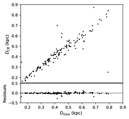
Figure 10: Comparisons of the distances derived from the PLZC relations and these from Gaia DR3. The residuals of distances is presented in below the sub-figure.

Stars in open clusters (OCs) have roughly the same age, distance, and chemical composition, while independent distances of OCs can be measured precisely. Most OCs located at high latitudes in the Milky Way are less effected by the extinction, which are preferred tools for testing calibrations. We derive the distances of CBs which are recognized as OCs membership or candidates. The name of the OCs are listed in the first column of Table 9, followed with their distances in the second column which are estimated through analyzing cluster memberships based on Gaia DR3 by Hunt & Reffert (2023). The $\rm RA$, $\rm Dec$ and periods of CBs as OCs membership (or candidates) are given in the 3-5th columns, while the corresponding literatures in the seventh column. The derived distances of the CBs ($D_{CB}$) are listed in the sixth column. The $\delta D$ in the last column presents the difference between $D_{OC}$ and $D_{CB}$ ($\delta D=D_{OC}-D_{CB}$). For the majority of the CBs, who are OC members, a comparison of the $D_{CB}$ and $D_{OC}$ reveals good agreement. For a certain CBs, the large discrepancies between $D_{CB}$ and $D_{OC}$ imply that those CBs are probably foreground or background sources of the OCs. For example, the two CBs in NGC 957 are more likely to be foreground stars in the cluster, which is consistent with the study of Luo et al. (2017).

Table 9: Distance comparisons of CBs and OCs.

Cluster	$D_{OC}$	RA	Dec	Period	$D_{CB}$	Ref. of membership or candidates	$\delta D$
	(pc)	(deg)	(deg)	(day)	(pc)		(pc)
NGC 957	2384 $\pm$ 620	38.595	57.429	0.40	872$\pm$46	Bukowiecki et al. (2009)	1512 $\pm$666
		38.108	57.445	0.31	674$\pm$84		1710 $\pm$704
NGC 1912	1140 $\pm$ 581	82.059	35.591	0.38	1541$\pm$19	Li et al. (2021)	$-$401 $\pm$600
		81.964	35.722	0.46	1028$\pm$84		112 $\pm$665
		82.299	35.722	0.38	1375$\pm$40		$-$235 $\pm$621
NGC 1245	3362$\pm$ 586	48.617	47.185	0.40	3308$\pm$10	Pepper & Burke (2006)	54 $\pm$596
King 7	3324 $\pm$ 282	60.270	51.361	0.36	698$\pm$59	Bukowiecki & Maciejewski (2008)	2626 $\pm$ 341
		60.200	51.196	0.29	2030$\pm$3		1294 $\pm$285
NGC 2126	1316 $\pm$ 287	90.895	49.612	0.44	1922$\pm$15	Liu et al. (2009)	$-$606 $\pm$302
NGC 2168	867 $\pm$ 679	92.371	24.117	0.39	2074$\pm$2	Hu et al. (2005)	$-$1207 $\pm$681
		91.779	24.401	0.32	1798$\pm$10		$-$931 $\pm$689
NGC 2355	1903 $\pm$ 370	109.349	13.781	0.31	1404$\pm$33	Wang et al. (2022)	499 $\pm$403
NGC 6819	2661$\pm$ 1115	296.165	40.080	0.30	1108$\pm$97	Li & Liu (2021)	1553 $\pm$1212
		294.929	40.147	0.44	387$\pm$33		2274 $\pm$1148
		295.196	40.350	0.46	2789$\pm$28		$-$128 $\pm$1143
		295.224	40.526	0.42	2035$\pm$44		626 $\pm$1159
NGC 6939	1905 $\pm$ 889	308.341	60.620	0.29	1732$\pm$23	Maciejewski et al. (2008)	173 $\pm$912
NGC 7142	2437 $\pm$ 522	326.118	65.776	0.33	270$\pm$14	Punanova et al. (2011)	2167 $\pm$536
NGC 7789	2087$\pm$ 1404	359.455	56.783	0.33	2086$\pm$25	Jahn et al. (1995)	1 $\pm$1429

4 Discussions and Conclusions

Considering relations between color index and stellar luminosity, as well as the influences of metallicity abundance on stellar radius and luminosity, PLZC relations for late-type CBs are calibrated based on current surveys and synthetic photometry. Starting with collecting CBs from photometry surveys and catalogs, we cross-match them with LAMOST and Gaia catalogs to obtain the spectroscopic data and distance information to construct a sample of 1093 CBs to calibrate. For the sample, PLZC relations for optical, infrared, and ultraviolet bands are derived. As comparisons, PL, PLZ, and PLC relations are also derived simultaneously. In addition to these relations for measured data, relations based on synthetic photometry are also calibrated.

Based on the PLZC relations of CBs for infrared and optical bands, distances could be measured with an accuracy of 6% (0.12 mag) and 8% (0.17 mag), respectively. In the optical bands, the dispersion of PLZC relations could be reduced to 6% (0.14 mag) when using the CBs sample with GSPC. In addition, the fitting results of FUV, NUV, W3, and W4-band are relatively poor, probably due to the small sampling rates of the observations. GALEX visits its targets with at least one epoch, mostly more than twice (Bianchi et al., 2017). W1 and W2-band have been observed with more than 30 epochs, while W3 and W4-band visited with $\sim$16 epochs (Wright et al., 2010). Gaia has made at least 15-epoch observations for its each band (Gaia Collaboration et al., 2023b).

Pollutions from other variables to CBs would affect the estimation of distances. Though variable stars such as RR Lyrae with periods ranging from 0.2 to 1.0 day have the similar periods to CBs, RR Lyrae with redder colors (than CBs) are easy to identify from CBs. As discussed in Drake et al. (2014), contamination (from RRc) leads to larger CB distances on the order of 1% (0.02 mag), which is lower than the uncertainty of calibrations in this work. Thus, pollutions from RR Lyrae are ignored here. A certain proportion of close binaries are accompanied by tertiary companions (Ruciński & Kaluzny, 1982; Hendry & Mochnacki, 1998), which is an important source of systemic uncertainty for calibrations and distance estimations. According to D’Angelo et al. (2006), the uncertainty in total luminosity introduced by a relatively bright tertiary is less than 15% (or 0.15 mag). The calibration uncertainties caused by tertiary companions could be reduced to $0.15/\sqrt{N}$ mag, where $N$ is the number of samples for calibration. Its typical value would be less than 0.01 mag for a sample with hundreds of CBs. The systemic uncertainty of distance estimation introduced by a faint tertiary star would be less than $\sim$7% even smaller. It is also expected to be effectively reduced by increasing samples. Since the sample for calibrations in this work are not tested for tertiary companions, the influence of tertiary companions is included in the calibrations by default.

Tests of the distances derived from PLZC relations with these from Gaia and literatures demonstrate the robust of the calibrations. Comparing the distances of CBs with the average distance of OCs could reveal whether the CBs are OCs memberships or not. Given the periods are well determined, the uncertainty of distances estimated based on the method depend on the uncertainties of photometry and extinction. Assuming the limiting magnitude of a photometry survey is about 24 mag (e.g. ESA’s Euclid mission’s step$-$and$-$stare survey strategy covers the full area to a depth of YJH $\sim$ 24 mag, Joachimi, 2016), the PLZC method could measure the CBs as far as 60 Kpc, which covers the distance of LMC (e.g. Chen et al., 2016).

Although considering the influence of [$\rm Fe/H$] and color index could improve the precision of model calibrations, it probably remains some improvements if the intrinsic luminosity are well studied from an theoretical view. In future work, we are going to analyze the Period-Luminosity-Color and Period-Luminosiy-Metallicity-Color relations based on stellar models and quantify the relations from a theoretical view.

References

- Abbott et al. (2016) Abbott, B. P., Abbott, R., Abbott, T. D., et al. 2016, Phys. Rev. X, 6, 041015, doi: 10.1103/PhysRevX.6.041015
- Abbott et al. (2017) Abbott, B. P., Abbott, R., Abbott, T. D., et al. 2017, ApJ, 848, L12, doi: 10.3847/2041-8213/aa91c9
- Arcones & Thielemann (2023) Arcones, A., & Thielemann, F.-K. 2023, A&A Rev., 31, 1, doi: 10.1007/s00159-022-00146-x
- Bessell & Murphy (2012) Bessell, M., & Murphy, S. 2012, PASP, 124, 140, doi: 10.1086/664083
- Bianchi et al. (2017) Bianchi, L., Shiao, B., & Thilker, D. 2017, ApJS, 230, 24, doi: 10.3847/1538-4365/aa7053
- Bukowiecki & Maciejewski (2008) Bukowiecki, L., & Maciejewski, G. 2008, Information Bulletin on Variable Stars, 5857, 1
- Bukowiecki et al. (2009) Bukowiecki, Ł., Maciejewski, G., Bykowski, W., et al. 2009, Open European Journal on Variable Stars, 112, 1
- Chen et al. (2016) Chen, X., de Grijs, R., & Deng, L. 2016, ApJ, 832, 138, doi: 10.3847/0004-637X/832/2/138
- Chen et al. (2018) Chen, X., Deng, L., de Grijs, R., Wang, S., & Feng, Y. 2018, ApJ, 859, 140, doi: 10.3847/1538-4357/aabe83
- Cowperthwaite et al. (2017) Cowperthwaite, P. S., Berger, E., Villar, V. A., et al. 2017, ApJ, 848, L17, doi: 10.3847/2041-8213/aa8fc7
- Cui et al. (2012) Cui, X.-Q., Zhao, Y.-H., Chu, Y.-Q., et al. 2012, Research in Astronomy and Astrophysics, 12, 1197, doi: 10.1088/1674-4527/12/9/003
- Cutri et al. (2021) Cutri, R. M., Wright, E. L., Conrow, T., et al. 2021, VizieR Online Data Catalog, II/328
- D’Angelo et al. (2006) D’Angelo, C., van Kerkwijk, M. H., & Rucinski, S. M. 2006, AJ, 132, 650, doi: 10.1086/505265
- De Angeli et al. (2022) De Angeli, F., Weiler, M., Montegriffo, P., et al. 2022, arXiv e-prints, arXiv:2206.06143. https://arxiv.org/abs/2206.06143
- Deng et al. (2012) Deng, L.-C., Newberg, H. J., Liu, C., et al. 2012, Research in Astronomy and Astrophysics, 12, 735, doi: 10.1088/1674-4527/12/7/003
- Devarapalli et al. (2020) Devarapalli, S. P., Jagirdar, R., Prasad, R. M., et al. 2020, MNRAS, 493, 1565, doi: 10.1093/mnras/staa031
- Drake et al. (2014) Drake, A. J., Graham, M. J., Djorgovski, S. G., et al. 2014, ApJS, 213, 9, doi: 10.1088/0067-0049/213/1/9
- Eggen (1967) Eggen, O. J. 1967, MmRAS, 70, 111
- Eggleton (1983) Eggleton, P. P. 1983, ApJ, 268, 368, doi: 10.1086/160960
- Eker et al. (2009) Eker, Z., Bilir, S., Yaz, E., Demircan, O., & Helvaci, M. 2009, Astronomische Nachrichten, 330, 68, doi: 10.1002/asna.200811041
- Fong & Berger (2013) Fong, W., & Berger, E. 2013, ApJ, 776, 18, doi: 10.1088/0004-637X/776/1/18
- Gaia Collaboration (2022) Gaia Collaboration. 2022, VizieR Online Data Catalog, I/355
- Gaia Collaboration et al. (2016) Gaia Collaboration, Brown, A. G. A., Vallenari, A., et al. 2016, A&A, 595, A2, doi: 10.1051/0004-6361/201629512
- Gaia Collaboration et al. (2023a) Gaia Collaboration, Montegriffo, P., Bellazzini, M., et al. 2023a, A&A, 674, A33, doi: 10.1051/0004-6361/202243709
- Gaia Collaboration et al. (2023b) Gaia Collaboration, Vallenari, A., Brown, A. G. A., et al. 2023b, A&A, 674, A1, doi: 10.1051/0004-6361/202243940
- Goodman & Weare (2010) Goodman, J., & Weare, J. 2010, Communications in Applied Mathematics and Computational Science, 5, doi: 10.2140/camcos.2010.5.65
- Graham et al. (2019) Graham, M. J., Kulkarni, S. R., Bellm, E. C., et al. 2019, PASP, 131, 078001, doi: 10.1088/1538-3873/ab006c
- Green et al. (2019) Green, G. M., Schlafly, E., Zucker, C., Speagle, J. S., & Finkbeiner, D. 2019, The Astrophysical Journal, 887, 93, doi: 10.3847/1538-4357/ab5362
- Hendry & Mochnacki (1998) Hendry, P. D., & Mochnacki, S. W. 1998, ApJ, 504, 978, doi: 10.1086/306126
- Hu et al. (2005) Hu, J.-H., Ip, W.-H., Zhang, X.-B., et al. 2005, Chinese J. Astron. Astrophys., 5, 356, doi: 10.1088/1009-9271/5/4/003
- Hunt & Reffert (2023) Hunt, E. L., & Reffert, S. 2023, A&A, 673, A114, doi: 10.1051/0004-6361/202346285
- Iben & Tutukov (1984) Iben, I., J., & Tutukov, A. V. 1984, ApJS, 54, 335, doi: 10.1086/190932
- Jahn et al. (1995) Jahn, K., Kaluzny, J., & Rucinski, S. M. 1995, A&A, 295, 101, doi: 10.48550/arXiv.astro-ph/9410015
- Jayasinghe et al. (2019) Jayasinghe, T., Stanek, K. Z., Kochanek, C. S., et al. 2019, Monthly Notices of the Royal Astronomical Society, 491, 13, doi: 10.1093/mnras/stz2711
- Jayasinghe et al. (2020) Jayasinghe, T., Stanek, K. Z., Kochanek, C. S., et al. 2020, MNRAS, 493, 4045, doi: 10.1093/mnras/staa518
- Jeong & Kim (2011) Jeong, J.-H., & Kim, C.-H. 2011, Journal of Astronomy and Space Sciences, 28, 163, doi: 10.5140/JASS.2011.28.3.163
- Joachimi (2016) Joachimi, B. 2016, in Astronomical Society of the Pacific Conference Series, Vol. 507, Multi-Object Spectroscopy in the Next Decade: Big Questions, Large Surveys, and Wide Fields, ed. I. Skillen, M. Balcells, & S. Trager, 401
- Jordi et al. (2010) Jordi, C., Gebran, M., Carrasco, J. M., et al. 2010, A&A, 523, A48, doi: 10.1051/0004-6361/201015441
- Kang et al. (2004) Kang, Y. W., Lee, H.-W., Hong, K. S., Kim, C.-H., & Guinan, E. F. 2004, AJ, 128, 846, doi: 10.1086/422706
- Kormendy et al. (2009) Kormendy, J., Fisher, D. B., Cornell, M. E., & Bender, R. 2009, ApJS, 182, 216, doi: 10.1088/0067-0049/182/1/216
- Li et al. (2021) Li, C.-Y., Esamdin, A., Zhang, Y., et al. 2021, Research in Astronomy and Astrophysics, 21, 068, doi: 10.1088/1674-4527/21/3/068
- Li & Liu (2021) Li, X. Z., & Liu, L. 2021, AJ, 161, 35, doi: 10.3847/1538-3881/abcb92
- Liu et al. (2009) Liu, S.-F., Wu, Z.-Y., Zhang, X.-B., et al. 2009, Research in Astronomy and Astrophysics, 9, 791, doi: 10.1088/1674-4527/9/7/008
- Liu et al. (2014) Liu, X. W., Yuan, H. B., Huo, Z. Y., et al. 2014, in Setting the scene for Gaia and LAMOST, ed. S. Feltzing, G. Zhao, N. A. Walton, & P. Whitelock, Vol. 298, 310–321, doi: 10.1017/S1743921313006510
- Lohr et al. (2015) Lohr, M. E., Norton, A. J., Payne, S. G., West, R. G., & Wheatley, P. J. 2015, A&A, 578, A136, doi: 10.1051/0004-6361/201525747
- Luo et al. (2015) Luo, A. L., Zhao, Y.-H., Zhao, G., et al. 2015, Research in Astronomy and Astrophysics, 15, 1095, doi: 10.1088/1674-4527/15/8/002
- Luo et al. (2017) Luo, C., Zhang, X., Deng, L., et al. 2017, New A, 52, 29, doi: 10.1016/j.newast.2016.10.005
- Lutz & Kelker (1973) Lutz, T. E., & Kelker, D. H. 1973, PASP, 85, 573, doi: 10.1086/129506
- Ma et al. (2022) Ma, S., Liu, J.-Z., Zhang, Y., Hu, Q., & Lü, G.-L. 2022, Research in Astronomy and Astrophysics, 22, 095017, doi: 10.1088/1674-4527/ac80ec
- Maciejewski et al. (2008) Maciejewski, G., Georgiev, T., & Niedzielski, A. 2008, Astronomische Nachrichten, 329, 387, doi: 10.1002/asna.200710889
- Magnier et al. (2020) Magnier, E. A., Schlafly, E. F., Finkbeiner, D. P., et al. 2020, ApJS, 251, 6, doi: 10.3847/1538-4365/abb82a
- Matsumoto & Metzger (2022) Matsumoto, T., & Metzger, B. D. 2022, ApJ, 938, 5, doi: 10.3847/1538-4357/ac6269
- Mochnacki (1981) Mochnacki, S. W. 1981, ApJ, 245, 650, doi: 10.1086/158841
- Nardiello et al. (2018) Nardiello, D., Libralato, M., Piotto, G., et al. 2018, MNRAS, 481, 3382, doi: 10.1093/mnras/sty2515
- Ngeow et al. (2021) Ngeow, C.-C., Liao, S.-H., Bellm, E. C., et al. 2021, AJ, 162, 63, doi: 10.3847/1538-3881/ac01ea
- Pancino et al. (2022) Pancino, E., Marrese, P. M., Marinoni, S., et al. 2022, A&A, 664, A109, doi: 10.1051/0004-6361/202243939
- Pepper & Burke (2006) Pepper, J., & Burke, C. J. 2006, AJ, 132, 1177, doi: 10.1086/505942
- Pietrzyński et al. (2013) Pietrzyński, G., Graczyk, D., Gieren, W., et al. 2013, Nature, 495, 76, doi: 10.1038/nature11878
- Punanova et al. (2011) Punanova, A. F., Popov, A. A., Krushinsky, V. V., et al. 2011, Peremennye Zvezdy Prilozhenie, 11, 32
- Rieke & Lebofsky (1985) Rieke, G. H., & Lebofsky, M. J. 1985, ApJ, 288, 618, doi: 10.1086/162827
- Ruciński (1995) Ruciński, S. 1995, PASP, 107, 648, doi: 10.1086/133603
- Ruciński (1974) Ruciński, S. M. 1974, Acta Astron., 24, 119
- Ruciński (1994) —. 1994, PASP, 106, 462, doi: 10.1086/133401
- Ruciński (2000) Ruciński, S. M. 2000, The Astronomical Journal, 120, 319, doi: 10.1086/301417
- Ruciński (2004) Ruciński, S. M. 2004, New A Rev., 48, 703, doi: 10.1016/j.newar.2004.03.005
- Ruciński & Duerbeck (1997) Ruciński, S. M., & Duerbeck, H. W. 1997, PASP, 109, 1340, doi: 10.1086/134014
- Ruciński & Kaluzny (1982) Ruciński, S. M., & Kaluzny, J. 1982, Ap&SS, 88, 433, doi: 10.1007/BF01092710
- Samus’ et al. (2017) Samus’, N. N., Kazarovets, E. V., Durlevich, O. V., Kireeva, N. N., & Pastukhova, E. N. 2017, Astronomy Reports, 61, 80, doi: 10.1134/S1063772917010085
- Shibata & Taniguchi (2006) Shibata, M., & Taniguchi, K. 2006, Phys. Rev. D, 73, 064027, doi: 10.1103/PhysRevD.73.064027
- Smartt et al. (2017) Smartt, S. J., Chen, T. W., Jerkstrand, A., et al. 2017, Nature, 551, 75, doi: 10.1038/nature24303
- Sun et al. (2020) Sun, W., Chen, X., Deng, L., & de Grijs, R. 2020, ApJS, 247, 50, doi: 10.3847/1538-4365/ab7894
- Thanjavur et al. (2021) Thanjavur, K., Ivezić, Ž., Allam, S. S., et al. 2021, MNRAS, 505, 5941, doi: 10.1093/mnras/stab1452
- Tylenda et al. (2011) Tylenda, R., Hajduk, M., Kamiński, T., et al. 2011, A&A, 528, A114, doi: 10.1051/0004-6361/201016221
- Wang et al. (2022) Wang, H., Zhang, Y., Zeng, X., et al. 2022, AJ, 164, 40, doi: 10.3847/1538-3881/ac755a
- Wang & Chen (2019) Wang, S., & Chen, X. 2019, ApJ, 877, 116, doi: 10.3847/1538-4357/ab1c61
- Wang et al. (2018) Wang, S., Chen, X., de Grijs, R., & Deng, L. 2018, ApJ, 852, 78, doi: 10.3847/1538-4357/aa9d99
- Webbink (1984) Webbink, R. F. 1984, ApJ, 277, 355, doi: 10.1086/161701
- Whelan & Iben (1973) Whelan, J., & Iben, Icko, J. 1973, ApJ, 186, 1007, doi: 10.1086/152565
- Wright et al. (2010) Wright, E. L., Eisenhardt, P. R. M., Mainzer, A. K., et al. 2010, AJ, 140, 1868, doi: 10.1088/0004-6256/140/6/1868
- Xiao & Yuan (2022) Xiao, K., & Yuan, H. 2022, AJ, 163, 185, doi: 10.3847/1538-3881/ac540a
- Yuan et al. (2015) Yuan, H.-B., Liu, X.-W., Huo, Z.-Y., et al. 2015, MNRAS, 448, 855, doi: 10.1093/mnras/stu2723
- Zhang & Yuan (2023) Zhang, R., & Yuan, H. 2023, ApJS, 264, 14, doi: 10.3847/1538-4365/ac9dfa
- Zhao et al. (2012) Zhao, G., Zhao, Y.-H., Chu, Y.-Q., Jing, Y.-P., & Deng, L.-C. 2012, Research in Astronomy and Astrophysics, 12, 723, doi: 10.1088/1674-4527/12/7/002