On the Expressive Power of a Variant of the Looped Transformer

Abstract

Besides natural language processing, transformers exhibit extraordinary performance in solving broader applications, including scientific computing and computer vision. Previous works try to explain this from the expressive power and capability perspectives that standard transformers are capable of performing some algorithms. To empower transformers with algorithmic capabilities and motivated by the recently proposed looped transformer (Yang et al., 2024; Giannou et al., 2023), we design a novel transformer block, dubbed Algorithm Transformer (abbreviated as AlgoFormer). Compared with the standard transformer and vanilla looped transformer, the proposed AlgoFormer can achieve significantly higher expressiveness in algorithm representation when using the same number of parameters. In particular, inspired by the structure of human-designed learning algorithms, our transformer block consists of a pre-transformer that is responsible for task pre-processing, a looped transformer for iterative optimization algorithms, and a post-transformer for producing the desired results after post-processing. We provide theoretical evidence of the expressive power of the AlgoFormer in solving some challenging problems, mirroring human-designed algorithms. Furthermore, some theoretical and empirical results are presented to show that the designed transformer has the potential to be smarter than human-designed algorithms. Experimental results demonstrate the empirical superiority of the proposed transformer in that it outperforms the standard transformer and vanilla looped transformer in some challenging tasks.

1 Introduction

The emergence of the transformer architecture (Vaswani et al., 2017) marks the onset of a new era in natural language processing. Transformer-based large language models (LLMs), such as BERT (Devlin et al., 2019) and GPT-3 (Brown et al., 2020), revolutionized impactful language-centric applications, including language translation (Vaswani et al., 2017; Raffel et al., 2020), text completion/generation (Radford et al., 2019; Brown et al., 2020), sentiment analysis (Devlin et al., 2019), and mathematical reasoning (Imani et al., 2023; Yu et al., 2024; Zheng et al., 2023). Beyond the initial surge in LLMs, these transformer-based models have found extensive applications in diverse domains such as computer vision (Dosovitskiy et al., 2021), time series (Li et al., 2019), bioinformatics (Zhang et al., 2023b), and addressing various physical problems (Cao, 2021). While many studies have concentrated on employing transformer-based models to tackle challenging real-world tasks, yielding superior performances compared to earlier models, the mathematical understanding of transformers remains incomplete.

The initial line of research interprets transformers as function approximators. Edelman et al. (2022) delve into the learnability and complexity of transformers for the class of sparse Boolean functions. Gurevych et al. (2022) explore the binary classification tasks, demonstrating that the transformer can circumvent the curse of dimensionality with a suitable hierarchical composition model for the posterior probability. Takakura & Suzuki (2023) investigate the approximation ability of transformers as sequence-to-sequence functions with infinite-dimensional inputs and outputs. They highlight that the transformer can avoid the curse of dimensionality under the smoothness conditions, due to the feature extraction and property sharing mechanism. However, viewing transformers solely as functional approximators, akin to feed-forward neural networks and convolutional neural networks, may not provide a fully satisfying understanding.

Another line of studies focuses on understanding transformers as algorithm learners. Garg et al. (2022) empirically investigate the performance of transformers in in-context learning, where the input tokens are input-label pairs generated from classical machine learning models, e.g., (sparse) linear regression and decision tree. They find that transformers can perform comparably as standard human-designed machine learning algorithms. Some subsequent works try to explain the phenomenon. Akyürek et al. (2023) characterize decoder-based transformer as employing stochastic gradient descent for linear regression. Bai et al. (2023) demonstrate that transformers can address statistical learning problems and employ algorithm selection, such as ridge regression, Lasso, and classification problems. Zhang et al. (2023a) and Huang et al. (2023) simplify the transformer model with reduced active parameters, yet reveal that the simplified transformer retains sufficient expressiveness for in-context linear regression problems. In Ahn et al. (2023), transformers are extended to implement preconditioned gradient descent. The looped transformer is proposed in (Giannou et al., 2023), and is shown to have the potential to perform basic operations (e.g., addition and multiplication), as well as implicitly learn iterative algorithms  (Yang et al., 2024). More related and interesting studies can be found in (Huang et al., 2023; Von Oswald et al., 2023; Mahankali et al., 2024; Sun et al., 2023).

In this paper, inspired by the recently proposed looped transformer (Yang et al., 2024; Giannou et al., 2023), we propose a novel transformer block, which we refer to as AlgoFormer, and strictly enforce it as an algorithm learner by regularizing its architecture. The transformer block consists of three sub-transformers, i.e., the pre-, looped, and post-transformers, designed to perform distinct roles. The pre-transformer is responsible for preprocessing the input data, and formulating it into some mathematical problems. The looped transformer acts as an iterative algorithm in solving the hidden problems. Finally, the post-transformer handles suitable postprocessing to produce the desired results. In contrast to standard transformers, the AlgoFormer is more likely to implement algorithms, due to its algorithmic structures shown in Figure 1.

Our main contributions can be summarized as follows:

• We introduce a novel transformer block (as shown in Figure 1), inspired by looped transformer (Yang et al., 2024; Giannou et al., 2023), namely the AlgoFormer. This block is designed as algorithm learners, mimicking the structure of human-designed algorithms. Compared with the standard transformer, AlgoFormer enjoys a lower parameter size but higher expressiveness in specific algorithmic learning tasks; Compared with the vanilla looped transformer, AlgoFormer can represent complex algorithms more efficiently; see Section 2.

• We theoretically show the expressive power of the AlgoFormer in solving three challenging tasks in implementing some practical human-designed algorithms (Theorems 3.1-3.3), including some task-specific pre- and post-processing, as well as the gradient descent; see Section 3.

• Beyond the gradient descent, we prove that the AlgoFormer can implement the (second-order) Newton’s method in linear regression problems (Theorem 4.1). While our results primarily focus on encoder-based transformers, we also extend our findings to decoder-based transformers (Theorem 4.2); see Section 4.

• We experimentally investigate the behavior of the AlgoFormer with different hyperparameters in handling some challenging in-context learning tasks. The empirical results support the stronger expressiveness and powerfulness of the AlgoFormer, compared with the standard transformer and vanilla looped transformer; see Section 5.

This paper is organized as follows. The motivation for the design of the transformer block, including a brief introduction to transformer layer architectures, the algorithmic structure of the proposed transformer block, and the advantages of lower parameter size and higher expressiveness, are presented in Section 2. We provide detailed results for the expressiveness of the designed AlgoFormer in tackling three challenging tasks, in Section 3. In Section 4, we additionally show that the designed transformer is capable of implementing Newton’s method, a second-order optimization algorithm, beyond the gradient descent. We also extend our results for decoder-only transformers, which can only access data in the previous tokens for regression. In Section 5, experimental results studying the behavior of the designed transformer block are reported. We also empirically compare it with the standard transformer and vanilla looped transformer. Some concluding remarks and potential works are discussed in Section 6.

2 Motivation

In this section, we mainly discuss the construction and intuition of the AlgoFormer. Its advantages over standard transformer is then conveyed. Before going into details, we first elaborate the mathematical definition of transformer layers.

2.1 Preliminaries

A One-layer transformer is mathematically formulated as

$$\begin{split}&\text{Attn}\left(\bm{X}\right)=\bm{X}+\sum_{i=1}^{h}\bm{W}_{V}^{(i)}\bm{X}\cdot\text{softmax}\left(\bm{X}^{\top}\bm{W}_{K}^{(i)\top}\bm{W}_{Q}^{(i)}\bm{X}\right),\\ &\text{TF}\left(\bm{X}\right)=\text{Attn}\left(\bm{X}\right)+\bm{W}_{2}\text{ReLU}\left(\bm{W}_{1}\text{Attn}\left(\bm{X}\right)+\bm{b}_{1}\right)+\bm{b}_{2},\end{split}$$ (1)

where $\bm{X}\in\mathbb{R}^{D\times N}$ is the input tokens; $h$ is the number of heads; $\{\bm{W}_{V}^{(i)},\bm{W}_{K}^{(i)},\bm{W}_{Q}^{(i)}\}$ denote value, key and query matrices at $i$-th head, respectively; $\{\bm{W}_{2},\bm{W}_{1},\bm{b}_{2},\bm{b}_{1}\}$ are parameters of the shallow feed-forward ReLU neural network. The attention layer with softmax activation function mostly exchanges information between different tokens by the attention mechanism. Subsequently, the feed-forward ReLU neural network applies nonlinear transformations to each token vector and extracts more complicated and versatile representations.

2.2 Algorithmic Structures of Transformers

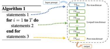
Figure 1: Algorithmic structure of the AlgoFormer. The pre-transformer conducts “statements 1” in the Algorithm; the looped transformer performs “statements 2” inner the for loop; the post-transformer carries out “statements 3”. Here, $\text{TF}_{\text{pre}}$, $\text{TF}_{\text{loop}}$, and $\text{TF}_{\text{post}}$ are multi-layer transformers; “statements” represent some fundamental operations in classical algorithms.

As discussed in the introduction, rather than simply interpreting it as a function approximator, the transformer may in-context execute some implicit algorithms learned from training data. However, it is still unverified that the standard multi-layer transformer is exactly performing algorithms.

Looped transformer. Although those works theoretically explain the success of transformers in solving (sparse) linear regression problems by the realization of (proximal) gradient descent, very little evidence implies that standard transformers are exactly implementing optimization algorithms. Note that the same mode of computation is conducted in each step of iteration. Equipped with the supposition that transformers can perform some basic operations, a shallow transformer is sufficient to represent iterative algorithms, as shown in the green part of Figure 1. The idea is first mentioned in Giannou et al. (2023), where they show that transformers can implement matrix addition and multiplication. Therefore, some iterative algorithms in scientific computing can be potentially realized by looped transformers. However, their construction does not explicitly imply the expressive power of transformers defined in Equation (1). Recently, Yang et al. (2024) empirically studied the behavior of looped transformers with different choices of hyperparameters in solving regression problems. Their experimental results further confirm the hypothesis that transformers are exactly learning iterative algorithms in solving linear regression problems, by strictly regularizing the transformer structure as looped transformers.

AlgoFormer. As shown in the green part of Figure 1, vanilla looped transformers (Yang et al., 2024; Giannou et al., 2023) admit the same structure as iterative algorithms, whose expressive power may be limited. However, real applications are usually much more complicated than linear regression problems. For example, given a task with data pairs, a well-trained researcher may first pre-process the data under some prior knowledge, and then formulate a mathematical (optimization) problem. Following that, some designed solvers, usually iterative algorithms, are performed. Finally, the desired results are obtained after further computation, namely, post-processing. The designed AlgoFormer (Algorithm Transformer), visualized in Figure 1, enjoys the same structure as wide classes of algorithms. Specifically, we separate the transformer block into three parts, i.e., pre-transformer $\text{TF}_{\text{pre}}$, looped transformer $\text{TF}_{\text{loop}}$, and post-transformer $\text{TF}_{\text{post}}$. Here, those three sub-transformers are standard multi-layer transformers in Equation (1). Given the input token vectors $\bm{X}$ and the number of iteration steps $T$, the output admits

$$\text{TF}_{\text{post}}\underbrace{\left(\text{TF}_{\text{loop}}\left(\cdots\text{TF}_{\text{loop}}\right.\right.}_{T\text{ iterations }}\left(\text{TF}_{\text{pre}}(\bm{X})\right))\cdots).$$ (2)

Compared with standard transformers, the AlgoFormer acts more as the algorithm learner, by strictly regularizing the loop structure. In comparison to the results presented in the previous work Giannou et al. (2023), our construction of AlgoFormer is closer to the transformer in real applications. In their approach, the design of the looped transformer necessitates task-specific knowledge, involving operations like token order switching. In contrast, our model is task-independent, emphasizing the learning of algorithms solely from data rather than relying on potentially unknown prior knowledge. In contrast to the looped transformer in Yang et al. (2024), we introduce pre- and post-transformers, which play essential roles in real applications, and the designed transformer block can represent complex algorithms and solve challenging tasks more efficiently.

Diffusion model. The looped transformer exhibits a structure similar to diffusion models (Sohl-Dickstein et al., 2015). This resemblance arises from the fact that diffusion models generate a clean image from a given noisy image, following a specific dynamical system governed by stochastic partial differential equations. It’s noteworthy that (iterative) optimization algorithms can also be viewed as a kind of dynamical system. Several related works leverage diffusion models for generating model parameters as meta-learners, simulating optimization dynamics (Krishnamoorthy et al., 2023; Peebles et al., 2022).

Meta-learner. The concept of a transformer as an algorithm learner shares connections with meta-learners like MAML (Finn et al., 2017) and Meta-SGD (Li et al., 2017). Meta-learners provide model parameters as initialization in a way that a small number of parameter updates and a limited amount of training samples are sufficient for achieving strong generalization performance on new tasks. Similarly, the AlgoFormer exhibits the capability to address new tasks with a modest number of (in-context) training samples.

2.3 Empirical Advantages

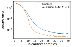
Figure 2: The validation error of trained models (the standard transformer and the AlgoFormer), assessed on sparse linear regression tasks. By choosing suitable hyperparameters (for example, we set $(T,\Delta T)=(12,10)$), defined in Equation (6), the proposed transformer has better performance than the standard transformer on the sparse linear regression.

In this subsection, we experimentally compare the performance of the AlgoFormer with the standard 12-layer transformer (i.e., GPT-2 model) in solving sparse linear regression. Note that from the algorithm learning perspective, the standard GPT-2 model can merely conduct at most 12 steps of computation, while our model exhibits higher expressive power with much lower parameter sizes but deeper loops. It is a significant advantage of the AlgoFormer, which enjoys algorithmic structures.

Lower parameter size. In the experiment, we adopt the transformer block where the three sub-transformers are all one-layer. Compared with the standard transformer (e.g., the GPT-2 model), our model is 4 times smaller in terms of the parameter size. It is imperative to note that our primary motivation was not centered around reducing the parameter size through weight sharing. Instead, our focus lies in enhancing the transformer’s role as an algorithm learner by incorporating algorithmic structures.

Higher expressiveness. Considering the (iterative) algorithm learning, in theory, the designed AlgoFormer admits even higher expressiveness than the GPT-2 model, although the latter enjoys more flexibility (large parameter size). It is also validated from the experiments (shown in Figure 2) that the designed transformer performs better than the standard transformer in sparse regression problems. The hard regularization on the transformer structure moves it closer to the algorithm learner. Note that the expressiveness of general weight-sharing models is often diminished due to their lower number of flexible parameters. However, the AlgoFormer demonstrates higher expressiveness, especially in specific iterative algorithm learning tasks, where the incorporation of deep loops plays a crucial role. In contrast to the vanilla looped transformer, the introduction of pre- and post-transformer components enables the transformer to learn more complicated and broader classes of algorithms.

Structure regularization. The transformer is intentionally designed with a structure similar to classical algorithms. The structure regularization of the transformer forces it to learn and conduct some implicit algorithms in solving in-context problems. In essence, it transforms the model into an explainable machine learning model, moving away from being a completely opaque, data-centric black-box model.

We conduct in-context learning of transformers on sparse linear regression problems. We compare the performances of the AlgoFormer (with different hyperparameters) and the GPT-2 model. As shown in Figure 2, for both two models, more in-context samples contribute to lower error, consistent with our intuition. In those simple examples, the designed AlgoFormer exhibits more competitive capabilities with the standard transformer. Due to the space limits, we put the details of the experiments in Appendix B.1. Further experiments on various tasks are presented in Section 5.

3 Expressive Power

In this section, we theoretically show by construction that AlgoFormer is capable of solving some challenging tasks, akin to human-designed algorithms. The core idea is as follows. Initially, the pre-transformer undertakes the crucial task of preprocessing the input data, such as representation transformation. The looped transformer is responsible for iterative algorithms in solving optimization problems. Finally, it is ready to output the desired result by the post-transformer. Through the analysis of AlgoFormer’s expressive power in addressing these tasks, we expect its potential to make contributions to the communities of scientific computing and machine learning.

3.1 Regression with Representation

We consider regression problems with representation, where the output behaves as a linear function of the input with a fixed representation function. Here, we adopt the $L$-layer MLPs with (leaky) ReLU activation function as the representation function $\Phi^{*}(\cdot)$. Specifically, we generate each in-context sample by first sampling the linear weight $\bm{A}$ from the prior $\mathcal{P}_{A}$, and then generating the input-label pair $\{(\bm{x}_{i},\bm{y}_{i})\}$ with $\bm{x}_{i}\in\mathbb{R}^{d}\sim\mathcal{P}_{x}$, $\bm{y}_{i}=\bm{A}\Phi^{*}(\bm{x}_{i})+\bm{\epsilon}_{i}$ and $\bm{\epsilon}_{i}\sim\mathcal{N}\left(\bm{0},\sigma^{2}\bm{I}\right)$. We aim to find the test label $\bm{y}_{\text{test}}:=\bm{A}\Phi^{*}(\bm{x}_{\text{test}})$, given the in-context samples and test data $\{\bm{x}_{1},\bm{y}_{1},\cdots,\bm{x}_{N},\bm{y}_{N},\bm{x}_{\text{test}}\}$. A reliable solver is expected first to identify the representation function and transform the input data $\bm{x}$ to its representation $\Phi^{*}(\bm{x})$. Then it reduces to a regression problem, and some optimization algorithms are performed to find the weight matrix from in-context samples. Finally, it outputs the desired result $\bm{y}_{\text{test}}$ by applying transformations on the test data. We prove by construction that there exists a AlgoFormer that solves the task, akin to the human-designed reliable solver.

Theorem 3.1.

There exists a designed AlgoFormer block with $\text{TF}_{\text{pre}}$ (an $(L+1)$-layer two-head transformer), $\text{TF}_{\text{loop}}$ (a one-layer two-head transformer), and $\text{TF}_{\text{post}}$ (a one-layer one-head transformer), that outputs $\bm{A}\Phi^{*}\left(\bm{x}_{\text{test}}\right)$ from the input-label pairs $\{\bm{x}_{1},\bm{y}_{1},\cdots,\bm{x}_{N},\bm{y}_{N},\bm{x}_{\text{test}}\}$ by fitting the representation function and applying gradient descent for multi-variate regression.

Remarks. The detailed proof is available in Appendix A.1. Our construction of the transformer block involves three distinct sub-transformers, each assigned specific responsibilities. The pre-transformer, characterized by identity attention, is dedicated to representation transformation through feed-forward neural networks. This stage reduces the task to a multivariate regression problem. Subsequently, the looped transformer operates in-context to determine the optimal weight, effectively acting as an iterative solver. Finally, the post-transformer is responsible for the post-processing and generate the desired result $\bm{A}\Phi^{*}\left(\bm{x}_{\text{test}}\right)$. Here, the input prompt to the transformer is formulated as

$$\bm{P}=\left[\begin{array}[]{ccccccc}\bm{x}_{1}&\bm{0}&\cdots&\bm{x}_{N}&\bm{0}&\bm{x}_{\text{test}}\\ \bm{0}&\bm{y}_{1}&\cdots&\bm{0}&\bm{y}_{N}&\bm{0}\\ \bm{p}_{1}^{x}&\bm{p}_{1}^{y}&\cdots&\bm{p}_{N}^{x}&\bm{p}_{N}^{y}&\bm{p}_{N+1}^{x}\end{array}\right],$$

where $\bm{p}_{i}^{x}$, and $\bm{p}_{i}^{y}$ denote positional embeddings and will be specified in the proof. Due to the differing dimensions of the input $\bm{x}$ and its corresponding label $\bm{y}$, zero padding is incorporated to reshape them into vectors of the same dimension. The structure of the prompt $\bm{P}$ aligns with similar formulations in previous works (Bai et al., 2023; Akyürek et al., 2023; Garg et al., 2022). For different input prompts $\bm{P}$, the hidden linear weights $\bm{A}$ are distinct but the representation function $\Phi^{*}(\cdot)$ is fixed. In comparison with the standard transformer adopted in Guo et al. (2024), which investigates similar tasks, the designed AlgoFormer has a significantly lower parameter size, making it closer to the envisioned human-designed algorithm. Notably, we construct the looped transformer to perform gradient descent for the multi-variate regression. However, the transformer exhibits remarkable versatility, as it has the capability to apply (ridge) regularized regression and more effective optimization algorithms beyond gradient descent. For more details, please refer to Section 4.

3.2 AR(q) with Representation

We consider the autoregressive model with representation. The dynamical (time series) system is generated by

$$\bm{x}_{t+1}=\bm{A}\Phi^{*}\left([\bm{x}_{t+1-q},\cdots,\bm{x}_{t}]\right)+\bm{\epsilon}_{t},$$

where $\Phi^{*}\left(\cdot\right)$ is a fixed representation function (e.g., we take the L-layer MLPs), and the weight $\bm{A}$ vary from different prompts. In standard AR(q) (multivariate autoregressive) models, the representation function $\Phi^{*}\left(\cdot\right)$ is identity. Here, we investigate a more challenging situation in which the representation function is fixed but unknown. A well-behaved solver should first find the representation function and then translate it into a modified autoregressive model. With standard Gaussian priors on the white noise $\bm{\epsilon}_{t}$, the Bayesian estimator of the AR(q) model parameters admits $\arg\max_{\bm{A}}\prod_{t=1}^{N}f(\bm{x}_{t}|\bm{x}_{t-1},\cdots,\bm{x}_{t-q})=\arg\min_{\bm{A}}\sum_{t=1}^{N}\left\|\bm{x}_{t}-\bm{A}\Phi^{*}\left([\bm{x}_{t-q},\cdots,\bm{x}_{t-1}]\right)\right\|_{2}^{2}$, where $f(\bm{x}_{t}|\bm{x}_{t-1},\cdots,\bm{x}_{t-q})$ is the conditional density function of $\bm{x}_{t}$, given previous $q$ observations. A practical solver initially identifies the representation function and transforms the input time series into its representation, denoted as $\Phi^{*}(\bm{x}_{t})$. Then the problem is reduced to an autoregressive form. Similar to the previous subsection, we prove by construction that there exists a AlgoFormer, akin to human-designed algorithms, capable of effectively solving the given task.

Theorem 3.2.

There exists a designed AlgoFormer block with $\text{TF}_{\text{pre}}$ (a one-layer $q$-head transformer with an $(L+1)$-layer one-head transformer), $\text{TF}_{\text{loop}}$ (a one-layer two-head transformer), and $\text{TF}_{\text{post}}$ (a one-layer one-head transformer), that predicts $\bm{x}_{N+1}$ from the data sequence $\{\bm{x}_{1},\bm{x}_{2},\cdots,\bm{x}_{N}\}$ by copying, transformation of the representation function and applying gradient descent for multi-variate regression.

Remarks. The detailed proof can be found in Appendix A.2. The technical details are similar to Theorem 3.1. Additionally, the pre-transformer copies the feature from the previous $q$ tokens, utilizing $q$ heads for parallel processing.

3.3 Chain-of-Thought with MLPs

Chain-of-Thought (CoT) demonstrates exceptional performances in mathematical reasoning and text generation (Wei et al., 2022). The success of CoT has been theoretically explored, shedding light on its effectiveness in toy cases (Li et al., 2023) and on its computational complexity (Feng et al., 2023). In this subsection, we revisit the intriguing toy examples of CoT generated by leaky ReLU MLPs, denoted as CoT with MLPs, as discussed in Li et al. (2023). We begin by constructing an L-layer MLP with leaky ReLU activation. For an initial data point $\bm{x}\sim\mathcal{P}_{x}$, the CoT point $\bm{s}^{\ell}$ represents the output of the $\ell$-th layer of the MLP. Consequently, the CoT sequence $\{\bm{x},\bm{s}^{1},\cdots,\bm{s}^{L}\}$ is exactly generated as the output of each (hidden) layer of the MLP. The target of CoT with MLPs problem is to find the next state $\hat{\bm{s}}^{\ell+1}$ based on the CoT samples $\{\bm{x}_{1},\bm{s}_{1}^{1},\cdots,\bm{s}_{1}^{L},\bm{x}_{2},\cdots,\bm{x}_{N},\bm{s}_{N}^{1},\cdots,\bm{s}_{N}^{L},\bm{x}_{\text{test}},\hat{\bm{s}}^{1},\cdots,\hat{\bm{s}}^{\ell}\}$, where $\{\hat{\bm{s}}^{1},\cdots,\hat{\bm{s}}^{\ell}\}$ denotes the CoT prompting of $\bm{x}_{\text{test}}$. We establish by construction in Theorem 3.3 that the AlgoFormer adeptly solves the CoT with MLPs problem, exhibiting a capability akin to human-designed algorithms.

Theorem 3.3.

There exists a designed AlgoFormer block with $\text{TF}_{\text{pre}}$ (a seven-layer two-head transformer), $\text{TF}_{\text{loop}}$ (a one-layer two-head transformer), and $\text{TF}_{\text{post}}$ (a one-layer one-head transformer), that finds $\hat{\bm{s}}^{\ell+1}$ from samples $\{\bm{x}_{1},\bm{s}_{1}^{1},\cdots,\bm{s}_{1}^{L},\bm{x}_{2},\cdots,\bm{x}_{N},\bm{s}_{N}^{1},\cdots,\bm{s}_{N}^{L},\bm{x}_{\text{test}},\hat{\bm{s}}^{1},\cdots,\hat{\bm{s}}^{\ell}\}$ by filtering and applying gradient descent for multi-variate regression.

Remarks. We put the proof in Appendix A.3. The pre-transformer first identifies the positional number $\ell$, and subsequently filters the input sequence into $\{\bm{s}_{1}^{\ell},\bm{s}_{1}^{\ell+1},\bm{s}_{2}^{\ell},\bm{s}_{2}^{\ell+1},\cdots,\bm{s}_{N}^{\ell},\bm{s}_{N}^{\ell+1},\hat{\bm{s}}^{\ell}\}$. This filtering transformation reduces the problem to a multi-variate regression problem. Compared with Li et al. (2023), where an assumption is made, we elaborate on the role of looped transformers in implementing gradient descent. While the CoT with MLPs may not be explicitly equivalent to CoT tasks in real applications, Theorem 3.3 somewhat implies the potential of the AlgoFormer in solving CoT-related problems.

4 Discussion

In this section, we provide complementary insights to the results discussed in Section 3. Firstly, as discussed in the remark following Theorem 3.1, we construct the looped transformer that employs gradient descent to solve (regularized) multi-variate regression problems. However, in practical scenarios, the adoption of more efficient optimization algorithms is often preferred. Investigating the expressive power of transformers beyond gradient descent is both intriguing and appealing. As stated in Theorem 4.1, we demonstrate that the AlgoFormer can proficiently implement Newton’s method for solving linear regression problems. Secondly, the definition in Equation (1) implies the encoder-based transformer. In practical applications, a decoder-based transformer with causal attention, as seen in models like GPT-2 (Radford et al., 2019), may also be favored. For completeness, it is also compelling to examine the behavior of decoder-based transformers in algorithmic learning. Our findings, presented in Theorem 4.2, reveal that the decoder-based transformer block can also implement gradient descent in linear regression problems. The primary distinction lies in the fact that the decoder-based transformer utilizes previously observed data to evaluate the gradient, while the encoder-based transformer calculates the gradient based on the full data samples.

4.1 Beyond the Gradient Descent

In the designed transformer block, the pre-transformer initially processes the input token, transforming it into an optimization problem. Subsequently, the looped transformer implements iterative algorithms, such as gradient descent, to solve the optimization problem. Finally, the post-transformer aggregates and outputs the desired results. While our construction currently adopts gradient descent as the solver for optimization problems, practical scenarios often witness the superiority of certain optimization algorithms over gradient descent. For example, Newton’s (second-order) methods enjoy superlinear convergence under some mild conditions, outperforming gradient descent with linear convergence. This raises a natural question:

Can the transformer implement algorithms beyond gradient descent, including higher-order optimization algorithms?

In this section, we address this question by demonstrating that the designed AlgoFormer can also realize Newton’s method in regression problems.

Consider the linear regression problem given by:

$$\arg\min_{\bm{w}}\frac{1}{2N}\sum_{i=1}^{N}\left(\bm{w}^{\top}\bm{x}_{i}-y_{i}\right)^{2}.$$ (3)

Denote $\bm{X}=\left[\bm{x}_{1},\bm{x}_{2},\cdots,\bm{x}_{N}\right]^{\top}\in\mathbb{R}^{N\times d}$, $\bm{y}=\left[y_{1},y_{2},\cdots,y_{N}\right]^{\top}\in\mathbb{R}^{N\times 1}$ and $\bm{S}=\bm{X}^{\top}\bm{X}$. A typical Newton’s method for linear regression problems follows the update scheme:

$$\begin{array}[]{ll}\bm{M}_{0}=\alpha\bm{S},\text{ where }\alpha\in\left(0,\frac{2}{\left\|\bm{S}\bm{S}^{\top}\right\|_{2}}\right],\\ \vspace{0.5em}\bm{M}_{k+1}=2\bm{M}_{k}-\bm{M}_{k}\bm{S}\bm{M}_{k},\\ \vspace{0.5em}\bm{w}_{0}^{\text{Newton }}=\bm{M}_{0}\bm{X}^{\top}\bm{y},\\ \bm{w}_{k+1}^{\text{Newton }}=\bm{M}_{k+1}\bm{X}^{\top}\bm{y}.\end{array}$$ (4)

As described in Söderström & Stewart (1974); Pan & Schreiber (1991), the above update scheme (Newton’s method) enjoys superlinear convergence, in contrast to the linear convergence of gradient descent. The following theorem states that Newton’s method in Equation (4) can be realized by the AlgoFormer.

Theorem 4.1.

There exists a designed AlgoFormer block with $\text{TF}_{\text{pre}}$ (a one-layer two-head transformer), $\text{TF}_{\text{loop}}$ (a one-layer two-head transformer), and $\text{TF}_{\text{post}}$ (a two-layer two-head transformer), that implements Newton’s method described by Equation (4) in solving regression problems.

Remarks. The proof can be found in Appendix A.4. The pre-transformer performs preparative tasks, such as copying from neighboring tokens. The looped-transformer is responsible for updating and calculating $\bm{M}_{k}\bm{x}_{i}$ for each token $\bm{x}_{i}$ at every step $k$. The post-transformer compute the final estimated weight $\bm{w}_{T}^{\text{Newton }}$ and outputs the desired the results $\bm{w}_{T}^{\text{Newton}\top}\bm{x}_{\text{test}}$, where $T$ is the iteration number in Equations (2) and (4). In a related study by Fu et al. (2023), similar topics are explored, indicating that transformers exactly perform higher-order optimization algorithms. However, our transformer architectures differ, and technical details are distinct. Empirically, as shown in Section 5.3 and Appendix B.3, we find that the transformer is smarter compared to some human-designed algorithms, such as Newton’s method.

4.2 Decoder-based Transformer

In the preceding analysis, the encoder-based AlgoFormer (with full attention) demonstrates its capability to solve problems by performing algorithms. Previous studies (Giannou et al., 2023; Bai et al., 2023; Zhang et al., 2023a; Huang et al., 2023; Ahn et al., 2023) also focus on the encoder-based models. We opted for an encoder-based transformer because full-batch data is available for estimating gradient and Hessian information. However, in practical applications, decoder-based models, like GPT-2, are sometimes more prevalent. In this subsection, we delve into the performance of the decoder-based model when executing iterative optimization algorithms, such as gradient descent, to solve regression problems. The results are intriguing, as the decoder-based transformer evaluates the gradient based on previously viewed data from earlier tokens.

We consider the linear regression problem in Equation (3). Due to the limitations of the decoder-based transformer, which can only access previous tokens, implementing iterative algorithms based on the entire batch data is not feasible. However, it is important to note that the current token in a decoder-based transformer can access data from all previous tokens. To predict the label $y_{i}$ based on the input prompt $\bm{P}^{i}=\left[\bm{x}_{1},y_{1},\cdots,\bm{x}_{i}\right]$, the empirical loss for the linear weight at $\bm{x}_{i}$ is given by

$$\bm{w}^{i}\in\arg\min_{\bm{w}}\mathcal{L}\left(\bm{w};\bm{P}^{i}\right):=\frac{1}{2(i-1)}\sum_{j=1}^{i-1}\left(\bm{w}^{\top}\bm{x}_{j}-y_{j}\right)^{2}.$$ (5)

In essence, the linear weight is estimated using accessible data from the previous tokens, reflecting the restricted information available in the decoder-based transformer.

Theorem 4.2.

There exists a designed AlgoFormer block with $\text{TF}_{\text{pre}}$ (a one-layer two-head transformer), $\text{TF}_{\text{loop}}$ (a one-layer two-head transformer), and $\text{TF}_{\text{post}}$ (a two-layer two-head transformer), that outputs $\bm{w}^{i\top}_{T}\bm{x}_{i}$ for each input data $\bm{x}_{i}$, where $\bm{w}_{T}^{i}$ comes from $\arg\min_{\bm{w}}\mathcal{L}\left(\bm{w};\bm{P}^{i}\right)$ after $T$ steps of gradient descent.

Remarks. The detailed proof is available in Appendix A.5. The technical details closely resemble those in Theorem 3.1, with the key distinction being that the decoder-based transformer can solely leverage data from previous tokens to determine the corresponding weight $\bm{w}^{i}$. Our findings align with those in Guo et al. (2024), although our transformer architectures and attention mechanisms differ. In a related study by Akyürek et al. (2023), similar topics are explored, demonstrating that the decoder-based transformer performs single-sample stochastic gradient descent, while our results exhibit greater strength with $\bm{w}^{i}\in\arg\min_{\bm{w}}\mathcal{L}\left(\bm{w};\bm{P}^{i}\right)$. The construction of a decoder-based transformer for representing Newton’s method is more challenging. We left it as a potential topic for future investigation.

5 Experiment

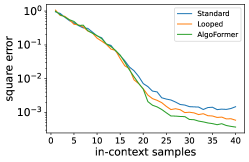
(a) Regression with representation

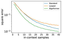
(b) AR(q) with representation

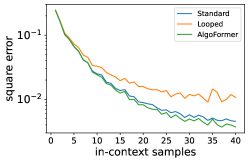
(c) CoT with MLPs

Figure 3: The validation error of trained models (the standard transformer, the vanilla looped transformer, and the AlgoFormer), assessed on regression with representation, AR(q) with representation, and CoT with MLPs tasks. By choosing suitable hyperparameters (i.e., we set $(T,\Delta T)=(20,15)$), the AlgoFormer has significantly better performance than the standard transformer and the vanilla looped transformer on those tasks.

In this section, we conduct a comprehensive empirical evaluation of the AlgoFormer’s performance in tackling challenging tasks, specifically addressing regression with representation, AR(q) with representation, and CoT with MLPs, as outlined in Section 2. Due to space limits, additional content has been provided in Appendix B. Before reporting the detailed experimental results, we provide an elaborate description of the experimental settings.

Experimental settings. In all experiments, we adopt the decoder-based AlgoFormer, standard transformer (GPT-2), and vanilla looped transformer (Yang et al., 2024). We utilize $N=40$ in-context samples as input prompts and $d=20$ dimensional vectors with $D=256$ dimensional positional embeddings for all experiments. To ensure fairness in comparisons, all models are trained using the Adam optimizer, with 500K iterations to ensure convergence. Both the pre- and post-transformers are implemented as one-layer transformers. For task-specific settings and additional details, please refer to Appendix B.1.

Training strategy. Our training strategy builds upon the methodology introduced in Yang et al. (2024). Let $\bm{P}^{i}=[\bm{x}_{1},f(\bm{x}_{1}),\cdots,\bm{x}_{i-1},f(\bm{x}_{i-1}),\bm{x}_{i}]$ represents the input prompt for $1\leq i\leq N$. We denote the AlgoFormer as $\text{TF}_{\text{Algo}}^{t}(\cdot;\bm{\Theta})$, where $f(\cdot)$ is a task-specific function and $t$ indicates the number of loops (iterations) in Equation (2), and $\bm{\Theta}$ represent the transformer parameters. Instead of evaluating the loss solely on $\text{TF}_{\text{Algo}}^{T}(\cdot;\bm{\Theta})$ with $T$ iterations, we minimize the expected loss over averaged iteration numbers:

$$\min_{\bm{\Theta}}\mathbb{E}_{\bm{P}}\left[\frac{1}{T-T_{0}}\sum_{t=T_{0}}^{T}\frac{1}{N}\sum_{i=1}^{N}\left\|\text{TF}_{\text{Algo}}^{t}(\bm{P}^{i};\bm{\Theta})-f(\bm{x}_{i})\right\|_{2}^{2}\right],$$ (6)

where $T_{0}=\max\{T-\Delta T,0\}$. Here, the prompt formulation and the above loss may slightly differ for different tasks. For example, in the AR(q) task, the prompt is reformulated as $\bm{P}^{i}=[\bm{x}_{1},\cdots,\bm{x}_{i-1},\bm{x}_{i}]$ and $\bm{x}_{i+1}=f([\bm{x}_{i+1-q},\cdots,\bm{x}_{i}])$ is the target for prediction. But the training strategy can be easily transmitted to other tasks. Here, both the iteration numbers $T_{0}$ and $T$ are hyperparameters, which will be analyzed in Appendix B.2.

5.1 AlgoFormer Exhibits Higher Expressiveness

In this subsection, we conduct a comparative analysis of the AlgoFormer against the standard and vanilla looped transformers across challenging tasks, as outlined in Section 3. Figure 3 illustrates the validation error trends, showcasing a decrease with an increasing number of in-context samples, aligning with our intuition. Crucially, the AlgoFormer consistently outperforms both the standard and the vanilla looped transformer across all tasks, highlighting its superior expressiveness in algorithm learning. Particularly in the CoT with MLPs task, both the AlgoFormer and the standard transformer significantly surpass the vanilla looped transformer. This further underscores the significance of preprocessing and postprocessing steps in handling complex real-world applications. The carefully designed algorithmic structure of the AlgoFormer emerges as an effective means of structural regularization, contributing to enhanced algorithm learning capabilities.

5.2 Impact of Hyperparameters

In this subsection, we conduct the empirical analysis of the impact of the hyperparameters on the AlgoFormer. The visualized results are provided in Appendix B.2. Notably, we observe that when training on higher values of $T$ and $\Delta T$, the AlgoFormer achieves stability with prolonged inference iterations. This observation suggests that the designed transformer exactly performs specific algorithms during its operation. However, it is important to note that larger values for $T$ and $\Delta T$ correspond to deeper transformers, leading to increased computational costs during both training and inference. On the contrary, smaller values for $T$ and $\Delta T$ may result in suboptimal performance. Striking a balance between the desired expressiveness and computational efficiency becomes imperative, highlighting the existence of a trade-off in these hyperparameters. Additionally, we investigate the influence of the number of heads and layers in the looped transformer $\text{TF}_{\text{loop}}$. We observe that a greater number of heads and layers contribute to the improved expressiveness, as shown in Figure 5. However, the overly many layers and heads may diminish the training and generalization.

5.3 Transformers May be Smarter than Human-Designed Algorithms

In this subsection, we leverage the AlgoFormer to address linear regression problems, presenting it as a pedagogical example for comparison with traditional methods such as gradient descent and Newton’s method. The hyperparameters in these experiments are detailed in Appendix B.3, with their selection grounded in a comprehensive grid search. According to the visualized results shown in Figure 6, transformers with fewer iterations outperform gradient descent and perform comparably and even better than Newton’s method. This observation suggests that transformers, through their strong expressiveness, may exhibit a higher level of algorithms compared to classical human-designed algorithms. Additional analyses and discussions on the transformers in algorithm learning comparing human-designed algorithms can be found in Appendix B.3.

6 Conclusion and Future Works

In this paper, we introduce a novel AlgoFormer, an algorithm learner designed from the looped transformer, distinguished by its algorithmic structures. Comprising three sub-transformers, each playing a distinct role in algorithm learning, the AlgoFormer demonstrates higher expressiveness while maintaining a lower parameter size compared to standard transformers. Moreover, AlgoFormer can represent algorithms more efficiently, in contrast to the vanilla looped transformer. Theoretical analysis establishes that the AlgoFormer can tackle challenging in-context learning tasks, mirroring human-designed algorithms. Our experiments further validate our claim, showing that the proposed transformer outperforms both the standard transformer and the vanilla looped transformer in specific algorithm learning tasks.

There are some potential topics for future research. For example, AlgoFormer exhibits a strikingly similar structure to diffusion models. This similarity arises from the fact that both the AlgoFormer (algorithms) and diffusion models draw inspiration from dynamical systems. Consequently, an interesting question arises: can the empirical training techniques and theoretical insights from the well-explored diffusion model literature be translated to the AlgoFormer for understanding the transformer mechanism?

Appendix A Technical Proof

In this section, we provide comprehensive proofs for all theorems stated in the main content.

Notation. We use boldface capital and lowercase letters to denote matrices and vectors respectively. Non-bold letters represent the elements of matrices or vectors, or scalers. For example, $A_{i,j}$ denotes the $(i,j)$-th element of the matrix $\bm{A}$. We use $\|\cdot\|_{2}$ to denote the 2-norm (or the maximal singular value) of a matrix.

A.1 Proof for Theorem 3.1

Positional embedding. The role of positional embedding is pivotal in the performance of transformers. Several studies have investigated its impact on natural language processing tasks, as referenced in (Kazemnejad et al., 2023; Ontanon et al., 2022; Press et al., 2022). In our theoretical construction, we deviate from empirical settings by using quasi-orthogonal vectors as positional embedding in each token vector. This choice, also employed by Li et al. (2023); Giannou et al. (2023), is made for theoretical convenience.

Lemma A.1 (Quasi-orthogonal vectors).

For any fixed $\epsilon>0$, there exists a set of vectors $\{\bm{p}_{1},\bm{p}_{2},\cdots,\bm{p}_{N}\}$ of dimension $\mathcal{O}\left(\log N\right)$ such that $\bm{p}_{i}^{\top}\bm{p}_{i}>\bm{p}_{i}^{\top}\bm{p}_{j}+\epsilon$ for all $i\neq j$.

Before going through the details, the following lemma is crucial for understanding transformers as algorithm learners.

Lemma A.2.

A one-layer two-head transformer exhibits the capability to implement a single step of gradient descent in multivariate regression.

Proof.

Let us consider the input prompt with positional embedding as follows:

$$\bm{P}:=\left[\begin{array}[]{ccccccc}\bm{x}_{1}&\bm{0}&\cdots&\bm{x}_{N}&\bm{0}&\bm{x}_{\text{test}}&\bm{0}\\ \bm{0}&\bm{y}_{1}&\cdots&\bm{0}&\bm{y}_{N}&\bm{0}&\bm{0}\\ \frac{1}{N}\bm{x}_{1}&\bm{0}&\cdots&\frac{1}{N}\bm{x}_{N}&\bm{0}&\bm{0}&\bm{0}\\ \bm{A}_{k}\bm{x}_{1}-\bm{y}_{1}&\bm{0}&\cdots&\bm{A}_{k}\bm{x}_{N}-\bm{y}_{N}&\bm{0}&\bm{A}_{k}\bm{x}_{\text{test}}&\bm{0}\\ 1&0&\cdots&1&0&1&0\\ 0&1&\cdots&0&1&0&1\\ 0&0&\cdots&0&0&1&0\\ 0&0&\cdots&0&0&0&1\end{array}\right],$$

where the 0-1 indicators are used to identify features, labels, and the test data, respectively. We denote the loss function for the multi-variate regression given samples $\{\bm{x}_{1},\bm{y}_{1},\cdots,\bm{x}_{N},\bm{y}_{N}\}$ as

$$\mathcal{L}\left(\bm{A}\right)=\frac{1}{2N}\sum_{j=1}^{N}\left\|\bm{A}\bm{x}_{j}-\bm{y}_{j}\right\|_{2}^{2},$$

then

$$\frac{\partial\mathcal{L}}{\partial\bm{A}}(\bm{A}_{k})=\frac{1}{N}\sum_{j=1}^{N}\left(\bm{A}_{k}\bm{x}_{j}-\bm{y}_{j}\right)\bm{x}_{j}^{\top}.$$

Now, let us define

$$\bm{W}_{Q}\bm{P}=\left[\begin{array}[]{ccccccc}c\bm{x}_{1}&\bm{0}&\cdots&c\bm{x}_{N}&\bm{0}&c\bm{x}_{\text{test}}&\bm{0}\\ 1&1&\cdots&1&1&1&1\end{array}\right],$$

$$\bm{W}_{K}\bm{P}=\left[\begin{array}[]{ccccccc}\frac{1}{N}\bm{x}_{1}&\bm{0}&\cdots&\frac{1}{N}\bm{x}_{N}&\bm{0}&\bm{0}&\bm{0}\\ 0&0&\cdots&0&0&0&C\end{array}\right],$$

and

$$\bm{W}_{V}\bm{P}=e^{C}\left[\begin{array}[]{ccccccc}\bm{A}_{k}\bm{x}_{1}-\bm{y}_{1}&\bm{0}&\cdots&\bm{A}_{k}\bm{x}_{N}-\bm{y}_{N}&\bm{0}&\bm{A}_{k}\bm{x}_{\text{test}}&\bm{0}\end{array}\right],$$

for some scalers $C,c>0$. Here, we denote

$$\bm{Z}:=\bm{P}^{\top}\bm{W}_{K}^{\top}\bm{W}_{Q}\bm{P}=\left[\begin{array}[]{ccccccc}\frac{c}{N}\bm{x}_{1}^{\top}\bm{x}_{1}&0&\cdots&\frac{c}{N}\bm{x}_{1}^{\top}\bm{x}_{N}&0&\frac{c}{N}\bm{x}_{1}^{\top}\bm{x}_{\text{test}}&0\\ \vdots&\vdots&\ddots&\vdots&\vdots&\vdots&\vdots\\ \frac{c}{N}\bm{x}_{N}^{\top}\bm{x}_{1}&0&\cdots&\frac{c}{N}\bm{x}_{N}^{\top}\bm{x}_{N}&0&\frac{c}{N}\bm{x}_{N}^{\top}\bm{x}_{\text{test}}&0\\ 0&0&\cdots&0&0&0&0\\ 0&0&\cdots&0&0&0&0\\ C&C&\cdots&C&C&C&C\end{array}\right],$$

then

$$e^{C}\cdot\text{softmax}\left(Z_{2i-1,2j-1}\right)\approx 1+\frac{c}{N}\bm{x}_{i}^{\top}\bm{x}_{j},$$

where the two sides of the “$\approx$” can be arbitrarily close if $C>0$ is sufficiently large and $c>0$ is sufficiently small. The constant here can be canceled by introducing another head. Therefore, the output of the attention layer is

$$\sum_{i=1}^{2}\bm{W}_{V}^{(i)}\bm{P}\cdot\text{softmax}\left(\bm{P}^{\top}\bm{W}_{K}^{(i)\top}\bm{W}_{Q}^{(i)}\bm{P}\right)\approx c\left[\begin{array}[]{ccccccc}\frac{\partial\mathcal{L}}{\partial\bm{A}}(\bm{A}_{k})\bm{x}_{1}&\bm{0}&\cdots&\frac{\partial\mathcal{L}}{\partial\bm{A}}(\bm{A}_{k})\bm{x}_{N}&\bm{0}&\frac{\partial\mathcal{L}}{\partial\bm{A}}(\bm{A}_{k})\bm{x}_{\text{test}}&\bm{0}\\ \end{array}\right].$$

The transformer layer’s output, after passing through the feed-forward neural network, is expressed as:

$$\left[\begin{array}[]{ccccccc}\bm{x}_{1}&\bm{0}&\cdots&\bm{x}_{N}&\bm{0}&\bm{x}_{\text{test}}&\bm{0}\\ \bm{0}&\bm{y}_{1}&\cdots&\bm{0}&\bm{y}_{N}&\bm{0}&\bm{0}\\ \bm{A}_{k+1}\bm{x}_{1}-\bm{y}_{1}&\bm{0}&\cdots&\bm{A}_{k+1}\bm{x}_{N}-\bm{y}_{N}&\bm{0}&\bm{A}_{k+1}\bm{x}_{\text{test}}&\bm{0}\\ 1&0&\cdots&1&0&1&0\\ 0&1&\cdots&0&1&0&1\\ 0&0&\cdots&0&0&1&0\\ 0&0&\cdots&0&0&0&1\end{array}\right].$$

This signifies the completion of one step of gradient descent with $\bm{A}_{k+1}=\bm{A}_{k}-\eta\frac{\partial\mathcal{L}}{\partial\bm{A}}(\bm{A}_{k})$ and a positive step size $\eta>0$. ∎

Proof for Theorem 3.1. We start by showing that $L$-layer transformer can represent $L$-layer MLPs. It is observed that the identity operation (i.e., $\text{Attn}\left(\bm{X}\right)=\bm{X}$) can be achieved by setting $\bm{W}_{V}=\bm{0}$ due to the residual connection in the attention layer. Each feed-forward neural network in a transformer layer can represent a one-layer MLP. Consequently, the representation function $\Phi^{*}(\cdot)$ can be realized by $L$-layer transformers. At the output layer of the $L$-th layer transformer, let $\bm{A}_{0}$ be an initial guess for the weight. The current output token vectors are then given by:

$$\bm{P}:=\left[\begin{array}[]{ccccccc}\Phi^{*}\left(\bm{x}_{1}\right)&\bm{0}&\cdots&\Phi^{*}\left(\bm{x}_{N}\right)&\bm{0}&\Phi^{*}\left(\bm{x}_{\text{test}}\right)&\bm{0}\\ \bm{0}&\bm{y}_{1}&\cdots&\bm{0}&\bm{y}_{N}&\bm{0}&\bm{0}\\ \bm{A}_{0}\Phi^{*}\left(\bm{x}_{1}\right)&\bm{0}&\cdots&\bm{A}_{0}\Phi^{*}\left(\bm{x}_{N}\right)&\bm{0}&\bm{A}_{k+1}\Phi^{*}\left(\bm{x}_{\text{test}}\right)&\bm{0}\\ \bm{p}_{1}&\bm{p}_{1}&\cdots&\bm{p}_{N}&\bm{p}_{N}&\bm{p}_{N+1}&\bm{p}_{N+1}\\ \frac{1}{N}&\frac{1}{N}&\cdots&\frac{1}{N}&\frac{1}{N}&0&0\\ 1&0&\cdots&1&0&1&0\\ 0&1&\cdots&0&1&0&1\\ 0&0&\cdots&0&0&1&0\\ 0&0&\cdots&0&0&0&1\end{array}\right].$$

Here, the set of quasi-orthogonal vectors $\{\bm{p}_{1},\cdots,\bm{p}_{N+1}\}$ is generated, according to Lemma A.1. The next transformer layer is designed to facilitate the exchange of information between neighboring tokens. Let

$$\bm{W}_{K}\bm{P}=\bm{W}_{Q}\bm{P}=\left[\begin{array}[]{ccccccc}\bm{p}_{1}&\bm{p}_{1}&\cdots&\bm{p}_{N}&\bm{p}_{N}&\bm{p}_{N+1}&\bm{p}_{N+1}\end{array}\right]$$

and

$$\bm{W}_{V}\bm{P}=\left[\begin{array}[]{ccccccc}\bm{0}&\bm{y}_{1}&\cdots&\bm{0}&\bm{y}_{N}&\bm{0}&\bm{0}\end{array}\right],$$

then

$$\bm{W}_{V}\bm{P}\cdot\text{softmax}\left(\bm{P}^{\top}\bm{W}_{K}^{\top}\bm{W}_{Q}\bm{P}\right)\approx\left[\begin{array}[]{ccccccc}\frac{1}{2}\bm{y}_{1}&\frac{1}{2}\bm{y}_{1}&\cdots&\frac{1}{2}\bm{y}_{N}&\frac{1}{2}\bm{y}_{N}&\bm{0}&\bm{0}\end{array}\right],$$

where the two sides of the “$\approx$” can be arbitrarily close if the temperature of the softmax function is sufficiently large, due to the nearly orthogonality of positional embedding vectors. It’s important to note that the feed-forward neural network is capable of approximating nonlinear functions, such as multiplication. Here, we construct a shallow neural network that calculates the multiplication between the first $d$ elements and the value $\frac{1}{N}$ in each token. Passing through the feed-forward neural network together with the indicators, we obtain the final output of the first $(L+1)$-layer transformer $\text{TF}_{\text{pre}}$:

$$\left[\begin{array}[]{ccccccc}\Phi^{*}\left(\bm{x}_{1}\right)&\bm{0}&\cdots&\Phi^{*}\left(\bm{x}_{N}\right)&\bm{0}&\Phi^{*}\left(\bm{x}_{\text{test}}\right)&\bm{0}\\ \bm{0}&\bm{y}_{1}&\cdots&\bm{0}&\bm{y}_{N}&\bm{0}&\bm{0}\\ \frac{1}{N}\Phi^{*}\left(\bm{x}_{1}\right)&\bm{0}&\cdots&\frac{1}{N}\Phi^{*}\left(\bm{x}_{N}\right)&\bm{0}&\bm{0}&\bm{0}\\ \bm{A}_{0}\Phi^{*}\left(\bm{x}_{1}\right)-\bm{y}_{1}&\bm{0}&\cdots&\bm{A}_{0}\Phi^{*}\left(\bm{x}_{N}\right)-\bm{y}_{N}&\bm{0}&\bm{A}_{0}\Phi^{*}\left(\bm{x}_{\text{test}}\right)&\bm{0}\\ \bm{p}_{1}&\bm{p}_{1}&\cdots&\bm{p}_{N}&\bm{p}_{N}&\bm{p}_{N+1}&\bm{p}_{N+1}\\ 1&0&\cdots&1&0&1&0\\ 0&1&\cdots&0&1&0&1\\ 0&0&\cdots&0&0&1&0\\ 0&0&\cdots&0&0&0&1\end{array}\right].$$

According to the construction outlined in Lemma A.2, there exists a one-layer, two-head transformer $\text{TF}_{\text{loop}}$, independent of the input data samples (tokens), that can implement gradient descent for finding the optimal weight $\bm{A}^{*}$ in the context of multivariate regression. The optimization aims to minimize the following empirical loss:

$$\min_{\bm{A}}\frac{1}{2N}\sum_{i=1}^{N}\left\|\bm{A}\Phi^{*}\left(\bm{x}_{i}\right)-\bm{y}_{i}\right\|_{2}^{2}.$$

After $k$-steps of looped transformer $\text{TF}_{\text{loop}}$, which corresponds to applying $k$ steps of gradient descent, the resulting token vectors follows

$$\left[\begin{array}[]{ccccccc}\Phi^{*}\left(\bm{x}_{1}\right)&\bm{0}&\cdots&\Phi^{*}\left(\bm{x}_{N}\right)&\bm{0}&\Phi^{*}\left(\bm{x}_{\text{test}}\right)&\bm{0}\\ \bm{0}&\bm{y}_{1}&\cdots&\bm{0}&\bm{y}_{N}&\bm{0}&\bm{0}\\ \frac{1}{N}\Phi^{*}\left(\bm{x}_{1}\right)&\bm{0}&\cdots&\frac{1}{N}\Phi^{*}\left(\bm{x}_{N}\right)&\bm{0}&\bm{0}&\bm{0}\\ \bm{A}_{k}\Phi^{*}\left(\bm{x}_{1}\right)-\bm{y}_{1}&\bm{0}&\cdots&\bm{A}_{k}\Phi^{*}\left(\bm{x}_{N}\right)-\bm{y}_{N}&\bm{0}&\bm{A}_{k}\Phi^{*}\left(\bm{x}_{\text{test}}\right)&\bm{0}\\ \bm{p}_{1}&\bm{p}_{1}&\cdots&\bm{p}_{N}&\bm{p}_{N}&\bm{p}_{N+1}&\bm{p}_{N+1}\\ 1&0&\cdots&1&0&1&0\\ 0&1&\cdots&0&1&0&1\\ 0&0&\cdots&0&0&1&0\\ 0&0&\cdots&0&0&0&1\end{array}\right].$$

These token vectors are then ready for processing by the output transformer layer $\text{TF}_{\text{post}}$. The post-transformer is designed to facilitate communication between the last two tokens and position the desired result $\bm{A}_{k}\Phi^{*}\left(\bm{x}_{\text{test}}\right)$ in the appropriate position. We can similarly set

$$\bm{W}_{K}\bm{P}=\bm{W}_{Q}\bm{P}=\left[\begin{array}[]{ccccccc}\bm{p}_{1}&\bm{p}_{1}&\cdots&\bm{p}_{N}&\bm{p}_{N}&\bm{p}_{N+1}&\bm{p}_{N+1}\end{array}\right],$$

$$\bm{W}_{V}\bm{P}=\left[\begin{array}[]{ccccccc}\bm{A}_{k}\Phi^{*}\left(\bm{x}_{1}\right)-\bm{y}_{1}&\bm{0}&\cdots&\bm{A}_{k}\Phi^{*}\left(\bm{x}_{N}\right)-\bm{y}_{N}&\bm{0}&\bm{A}_{k}\Phi^{*}\left(\bm{x}_{\text{test}}\right)&\bm{0}\end{array}\right],$$

and pass it through the feed-forward neural network. This results in the final output:

$$\left[\begin{array}[]{ccccccc}\Phi^{*}\left(\bm{x}_{1}\right)&\bm{0}&\cdots&\Phi^{*}\left(\bm{x}_{N}\right)&\bm{0}&\Phi^{*}\left(\bm{x}_{\text{test}}\right)&\bm{0}\\ \bm{0}&\bm{y}_{1}&\cdots&\bm{0}&\bm{y}_{N}&\bm{0}&\bm{A}_{k}\Phi^{*}\left(\bm{x}_{\text{test}}\right)\end{array}\right],$$

which completes the proof.

A.2 Proof for Theorem 3.2

The following lemma highlights the intrinsic “copying” capability of transformers, a pivotal feature for autoregressive models, especially in the context of time series analysis.

Lemma A.3.

A one-layer transformer with $q$ heads possesses the ability to effectively copy information from the previous $q$ tokens to the present token.

Proof.

We construct the input prompt with positional embedding as follows:

$$\left[\begin{array}[]{ccccc}\bm{x}_{0}&\bm{x}_{1}&\bm{x}_{2}&\cdots&\bm{x}_{N}\\ \bm{p}_{0}&\bm{p}_{1}&\bm{p}_{2}&\cdots&\bm{p}_{N}\\ \bm{p}_{-1}&\bm{p}_{0}&\bm{p}_{1}&\cdots&\bm{p}_{N-1}\\ \vdots&\vdots&\vdots&\ddots&\vdots\\ \bm{p}_{-q}&\bm{p}_{1-q}&\bm{p}_{2-q}&\cdots&\bm{p}_{N-q}\\ 0&1&2&\cdots&N\end{array}\right].$$

The i-th head aims to connect and communicate the current token with the previous $i$-th token. Specifically, we let

$$\bm{W}_{K}^{(i)}\bm{P}=\left[\begin{array}[]{ccccc}\bm{p}_{0}&\bm{p}_{1}&\bm{p}_{2}&\cdots&\bm{p}_{N}\end{array}\right],$$

$$\bm{W}_{Q}^{(i)}\bm{P}=\left[\begin{array}[]{ccccc}\bm{p}_{-i}&\bm{p}_{1-i}&\bm{p}_{2-i}&\cdots&\bm{p}_{N-i}\end{array}\right],$$

and

$$\bm{W}_{V}^{(i)}\bm{P}=\left[\begin{array}[]{cccccc}\bm{x}_{0}&\bm{x}_{1}&\bm{x}_{2}&\cdots&\bm{x}_{N}\end{array}\right],$$

we have

$$\bm{W}_{V}^{(i)}\bm{P}\cdot\text{softmax}\left(\bm{P}^{\top}\bm{W}_{K}^{(i)\top}\bm{W}_{Q}^{(i)}\bm{P}\right)\approx\left[\begin{array}[]{cccccc}*&\bm{x}_{1-i}&\bm{x}_{2-i}&\cdots&\bm{x}_{N-i}\end{array}\right].$$

Here, we use “*” to mask some unimportant token values. Therefore, the $q$-head attention layer outputs

$$\left[\begin{array}[]{cccccc}\bm{x}_{0}&\bm{x}_{1}&\bm{x}_{2}&\cdots&\bm{x}_{N}\\ &\bm{x}_{0}&\bm{x}_{1}&\cdots&\bm{x}_{N-1}\\ &*&\bm{x}_{0}&\cdots&\bm{x}_{N-2}\\ \vdots&\vdots&\vdots&\ddots&\vdots\\ &*&*&\cdots&\bm{x}_{N-q}\\ 0&1&2&\cdots&N\end{array}\right].$$

Here, the samples are only supported on $\{\bm{x}_{t}\}$ with $0\leq t\leq N$. It is common to alternatively define $\bm{x}_{t}=\bm{0}$ for $t<0$. Passing through the feed-forward neural network, together with the indicators at the last row, we can filter out the undefined elements, i.e.,

$$\left[\begin{array}[]{cccccc}\bm{x}_{0}&\bm{x}_{1}&\bm{x}_{2}&\cdots&\bm{x}_{N}\\ \bm{0}&\bm{x}_{0}&\bm{x}_{1}&\cdots&\bm{x}_{N-1}\\ \bm{0}&\bm{0}&\bm{x}_{0}&\cdots&\bm{x}_{N-2}\\ \vdots&\vdots&\vdots&\ddots&\vdots\\ \bm{0}&\bm{0}&\bm{0}&\cdots&\bm{x}_{N-q}\\ 0&1&2&\cdots&N\end{array}\right].$$

∎

Proof for Theorem 3.2 According to Lemma A.3 and Theorem 3.1, the $(L+2)$-layer pre-transformer $\text{TF}_{\text{pre}}$ is able to do copying and transformation of the representation function. The output after the preprocessing is given by

$$\left[\begin{array}[]{cccccc}\bm{x}_{0}&\bm{x}_{1}&\bm{x}_{2}&\cdots&\bm{x}_{N}\\ \Phi^{*}\left(\bm{x}_{1-q:0}\right)&\Phi^{*}\left(\bm{x}_{2-q:1}\right)&\Phi^{*}\left(\bm{x}_{3-q:2}\right)&\cdots&\Phi^{*}\left(\bm{x}_{N+1-q:N}\right)\end{array}\right],$$

where we denote $\bm{x}_{i:j}$ as the concatenation $[\bm{x}_{i},\bm{x}_{i+1},\cdots,\bm{x}_{j}]$ for notational simplicity. Similar to the construction in Lemma A.2, a one-layer two-head transformer $\text{TF}_{\text{loop}}$ is capable of implementing gradient descent on the multivariate regression. Finally, the post-transformer $\text{TF}_{\text{post}}$ moves the desired result to the output.

A.3 Proof for Theorem 3.3

According to Lemma 5 in (Li et al., 2023), a seven-layer, two-head pre-transformer $\text{TF}_{\text{pre}}$ is introduced for preprocessing the input CoT sequence. This pre-transformer performs filtering, transforming the input sequence into the structured form given by Equation (7).

$$\left[\begin{array}[]{cccccccccccc}\bm{0}&\cdots&\bm{s}_{1}^{\ell-1}&\bm{0}&\cdots&\bm{s}_{2}^{\ell-1}&\bm{0}&\cdots&\bm{0}&\bm{0}&\cdots&\hat{\bm{s}}^{\ell-1}\\ \bm{0}&\cdots&\bm{0}&\bm{s}_{1}^{\ell}&\cdots&\bm{0}&\bm{s}_{2}^{\ell}&\cdots&\bm{0}&\bm{0}&\cdots&\bm{0}\\ 0&\cdots&1&0&\cdots&1&0&\cdots&0&0&\cdots&1\\ 0&\cdots&0&1&\cdots&0&1&\cdots&0&0&\cdots&0\\ 0&\cdots&0&0&\cdots&0&0&\cdots&0&0&\cdots&1\\ \end{array}\right].$$ (7)

Specifically, it identifies the positional index $\ell-1$ of the last token $\hat{\bm{s}}^{\ell-1}$, retains only $\bm{s}_{i}^{\ell-1}$ and $\bm{s}_{i}^{\ell}$ for $1\leq i\leq N$, and filters out all other irrelevant tokens. In this context, the representation function $\Phi^{*}(\cdot)$ corresponds to $L$-layer leaky ReLU MLPs. Notably, the transformation $\bm{s}{i}^{\ell}=\sigma\left(\bm{W}^{\ell}\bm{s}{i}^{\ell-1}\right)$ is expressed, where $\bm{W}^{\ell}$ denotes the weight matrix at the $\ell$-th layer, and $\sigma(\cdot)$ represents the leaky ReLU activation function. Given the reversibility and piecewise linearity of the leaky ReLU activation, we can assume, without loss of generality, that $\bm{s}_{i}^{\ell}=\bm{W}^{\ell}\bm{s}_{i}^{\ell-1}$ in Equation (7). Consequently, the problem is reduced to a multi-variate regression, and a one-layer two-head transformer $\text{TF}_{\text{loop}}$ is demonstrated to effectively implement gradient descent for determining the weight matrix $\bm{W}^{\ell}$, as shown in Lemma A.2. Subsequently, the post-transformer $\text{TF}_{\text{post}}$ produces the desired result $\sigma\left(\bm{W}^{\ell}\hat{\bm{s}}{i}^{\ell-1}\right)$.

A.4 Proof for Theorem 4.1

In this section, we first show that the one-layer two-head transformer can implement a single step of Newton’s method in Equation (4), with the special form of input token vectors. Then, we introduce the pre-transformer, designed to convert general input tokens into the prescribed format conducive to the transformer’s operation. Finally, the post-transformer facilitates the extraction of the desired results through additional computations, given that the output from the looped-transformer corresponds to an intermediate product.

Lemma A.4.

A transformer with one layer and two heads is capable of implementing one step of Newton’s method in the linear regression problem in Equation (3).

Proof.

Let us consider the input prompt with positional embedding as follows:

$$\bm{P}:=\left[\begin{array}[]{ccccccc}\bm{x}_{1}&\bm{0}&\cdots&\bm{x}_{N}&\bm{0}&\bm{x}_{\text{test}}&\bm{0}\\ 0&y_{1}&\cdots&0&y_{N}&0&0\\ \bm{M}_{k}\bm{x}_{1}&\bm{0}&\cdots&\bm{M}_{k}\bm{x}_{N}&\bm{0}&\bm{0}&\bm{0}\\ 1&0&\cdots&1&0&0&0\\ 0&1&\cdots&0&1&0&0\\ 0&0&\cdots&0&0&1&0\\ 0&0&\cdots&0&0&0&1\\ \end{array}\right].$$

Let

$$\bm{W}_{Q}\bm{P}=\left[\begin{array}[]{ccccccc}\bm{M}_{k}\bm{x}_{1}&\bm{0}&\cdots&\bm{M}_{k}\bm{x}_{N}&\bm{0}&\bm{0}&\bm{0}\\ 1&1&\cdots&1&1&1&1\\ \end{array}\right],$$

$$\bm{W}_{K}\bm{P}=\left[\begin{array}[]{ccccccc}c\bm{x}_{1}&\bm{0}&\cdots&c\bm{x}_{N}&\bm{0}&c\bm{x}_{\text{test}}&\bm{0}\\ 0&0&\cdots&0&0&0&C\\ \end{array}\right],$$

and

$$\bm{W}_{V}\bm{P}=e^{C}\left[\begin{array}[]{ccccccc}\bm{M}_{k}\bm{x}_{1}&\bm{0}&\cdots&\bm{M}_{k}\bm{x}_{N}&\bm{0}&\bm{0}&\bm{0}\end{array}\right].$$

Similarly, denote $\bm{Z}:=\bm{P}^{\top}\bm{W}_{K}^{\top}\bm{W}_{Q}\bm{P}$, we can establish that

$$e^{C}\text{softmax}\left(Z_{2i-1,2j-1}\right)\approx 1+c\bm{x}_{i}^{\top}\bm{M}_{k}\bm{x}_{j}.$$ (8)

To nullify the constant term, an additional attention head can be incorporated. Therefore, the output takes the form:

$$\bm{W}_{V}\bm{P}\text{softmax}\left(\bm{P}^{\top}\bm{W}_{K}^{\top}\bm{W}_{Q}\bm{P}\right)\approx\left[\begin{array}[]{ccccccc}c\bm{M}_{k}\bm{S}\bm{M}_{k}\bm{x}_{1}&*&\cdots&c\bm{M}_{k}\bm{S}\bm{M}_{k}\bm{x}_{N}&*&*\end{array}\right].$$

Here, we use “*” to mask some unimportant token values. Upon passing through the feed-forward neural network with indicator $\left[\begin{array}[]{ccccccc}1&0&\cdots&1&0&0&0\end{array}\right]$ and weight $1/c$, the resulting output is

$$\left[\begin{array}[]{ccccccc}\bm{x}_{1}&\bm{0}&\cdots&\bm{x}_{N}&\bm{0}&\bm{x}_{\text{test}}&\bm{0}\\ 0&y_{1}&\cdots&0&y_{N}&0&0\\ \bm{M}_{k+1}\bm{x}_{1}&\bm{0}&\cdots&\bm{M}_{k+1}\bm{x}_{N}&\bm{0}&\bm{0}&\bm{0}\\ 1&0&\cdots&1&0&0&0\\ 0&1&\cdots&0&1&0&0\\ 0&0&\cdots&0&0&1&0\\ 0&0&\cdots&0&0&0&1\\ \end{array}\right],$$

where $\bm{M}_{k+1}=2\bm{M}_{k}-\bm{M}_{k}\bm{S}\bm{M}_{k}$. ∎

Proof for Theorem 4.1. For $\text{TF}_{\text{pre}}$, we adopt the following configurations:

$$\bm{W}_{Q}\bm{P}=\left[\begin{array}[]{ccccccc}\bm{x}_{1}&\bm{0}&\cdots&\bm{x}_{N}&\bm{0}&\bm{0}&\bm{0}\\ 1&1&\cdots&1&1&1&1\\ \end{array}\right],$$

$$\bm{W}_{K}\bm{P}=\left[\begin{array}[]{ccccccc}c\bm{x}_{1}&\bm{0}&\cdots&c\bm{x}_{N}&\bm{0}&c\bm{x}_{\text{test}}&\bm{0}\\ 0&0&\cdots&0&0&0&C\\ \end{array}\right],$$

and

$$\bm{W}_{V}\bm{P}=e^{C}\left[\begin{array}[]{ccccccc}\bm{x}_{1}&\bm{0}&\cdots&\bm{x}_{N}&\bm{0}&\bm{0}&\bm{0}\end{array}\right].$$

Denote $\bm{Z}:=\bm{P}^{\top}\bm{W}_{K}^{\top}\bm{W}_{Q}\bm{P}$, we can show that

$$e^{C}\text{softmax}\left(Z_{2i-1,2j-1}\right)\approx 1+c\bm{x}_{i}^{\top}\bm{x}_{j}.$$

We may include another attention head to remove the constant. Therefore, the output is formulated as

$$\bm{W}_{V}\bm{P}\text{softmax}\left(\bm{P}^{\top}\bm{W}_{K}^{\top}\bm{W}_{Q}\bm{P}\right)\approx\left[\begin{array}[]{ccccccc}c\bm{S}\bm{x}_{1}&*&\cdots&c\bm{S}\bm{x}_{N}&*&*\end{array}\right].$$

After passing through the feed-forward neural network with indicators $\left[\begin{array}[]{ccccccc}1&0&\cdots&1&0&0&0\end{array}\right]$ and weight $\alpha/c$, the resulting output becomes:

$$\left[\begin{array}[]{ccccccc}\bm{x}_{1}&\bm{0}&\cdots&\bm{x}_{N}&\bm{0}&\bm{x}_{\text{test}}&\bm{0}\\ 0&y_{1}&\cdots&0&y_{N}&0&0\\ \bm{M}_{0}\bm{x}_{1}&\bm{0}&\cdots&\bm{M}_{0}\bm{x}_{N}&\bm{0}&\bm{0}&\bm{0}\\ 1&0&\cdots&1&0&0&0\\ 0&1&\cdots&0&1&0&0\\ 0&0&\cdots&0&0&1&0\\ 0&0&\cdots&0&0&0&1\\ \end{array}\right],$$

where $\bm{M}_{0}=\alpha\bm{S}$.

As illustrated in Lemma A.4, after $T$ iterations of the looped transformer $\text{TF}_{\text{loop}}$, it produces the following output:

$$\left[\begin{array}[]{ccccccc}\bm{x}_{1}&\bm{0}&\cdots&\bm{x}_{N}&\bm{0}&\bm{x}_{\text{test}}&\bm{0}\\ 0&y_{1}&\cdots&0&y_{N}&0&0\\ \bm{M}_{T}\bm{x}_{1}&\bm{0}&\cdots&\bm{M}_{T}\bm{x}_{N}&\bm{0}&\bm{0}&\bm{0}\\ 1&0&\cdots&1&0&0&0\\ 0&1&\cdots&0&1&0&0\\ 0&0&\cdots&0&0&1&0\\ 0&0&\cdots&0&0&0&1\\ \end{array}\right].$$

In the post-transformer, additional positional embeddings are introduced to address technical considerations. The input is structured as follows:

$$\left[\begin{array}[]{ccccccc}\bm{x}_{1}&\bm{0}&\cdots&\bm{x}_{N}&\bm{0}&\bm{x}_{\text{test}}&\bm{0}\\ 0&y_{1}&\cdots&0&y_{N}&0&0\\ \bm{M}_{T}\bm{x}_{1}&\bm{0}&\cdots&\bm{M}_{T}\bm{x}_{N}&\bm{0}&\bm{0}&\bm{0}\\ \bm{p}_{1}&\bm{p}_{1}&\cdots&\bm{p}_{N}&\bm{p}_{N}&\bm{p}_{N+1}&\bm{p}_{N+1}\\ 1&0&\cdots&1&0&0&0\\ 0&1&\cdots&0&1&0&0\\ 0&0&\cdots&0&0&1&0\\ 0&0&\cdots&0&0&0&1\end{array}\right],$$

where the positional embedding vectors $\bm{p}_{1},\cdots,\bm{p}_{N+1}$ are designed to be nearly orthogonal (Lemma A.1). To initiate the weight $\bm{w}^{\text{Newton}}_{T}$, we propagate the target label $y$ to adjacent tokens using the following attention mechanism:

$$\bm{W}_{K}\bm{P}=\bm{W}_{Q}\bm{P}=\left[\begin{array}[]{ccccccc}\bm{p}_{1}&\bm{p}_{1}&\cdots&\bm{p}_{N}&\bm{p}_{N}&\bm{p}_{N+1}&\bm{p}_{N+1}\end{array}\right]$$

and

$$\bm{W}_{V}\bm{P}=2\left[\begin{array}[]{ccccccc}0&y_{1}&\cdots&0&y_{N}&0&0\end{array}\right].$$

This operation results in the attention layer producing the following output:

$$\left[\begin{array}[]{ccccccc}\bm{x}_{1}&\bm{0}&\cdots&\bm{x}_{N}&\bm{0}&\bm{x}_{\text{test}}&\bm{0}\\ y_{1}&y_{1}&\cdots&y_{N}&y_{N}&0&0\\ \bm{M}_{T}\bm{x}_{1}&\bm{0}&\cdots&\bm{M}_{T}\bm{x}_{N}&\bm{0}&\bm{0}&\bm{0}\\ \bm{p}_{1}&\bm{p}_{1}&\cdots&\bm{p}_{N}&\bm{p}_{N}&\bm{p}_{N+1}&\bm{p}_{N+1}\\ 1&0&\cdots&1&0&0&0\\ 0&1&\cdots&0&1&0&0\\ 0&0&\cdots&0&0&1&0\\ 0&0&\cdots&0&0&0&1\end{array}\right].$$

In the next layer, analogous to the construction in Equation (8), we define the following transformations:

$$\bm{W}_{Q}\bm{P}=\left[\begin{array}[]{ccccccc}c\bm{x}_{1}&\bm{0}&\cdots&c\bm{x}_{N}&\bm{0}&c\bm{x}_{\text{test}}&\bm{0}\\ 1&1&\cdots&1&1&1&1\end{array}\right],$$

$$\bm{W}_{K}\bm{P}=\left[\begin{array}[]{ccccccc}\bm{M}_{T}\bm{x}_{1}&\bm{0}&\cdots&\bm{M}_{T}\bm{x}_{N}&\bm{0}&\bm{0}&\bm{0}\\ 0&0&\cdots&0&0&0&C\end{array}\right],$$

and

$$\bm{W}_{V}\bm{P}=e^{C}\left[\begin{array}[]{ccccccc}y_{1}&y_{1}&\cdots&y_{N}&y_{N}&0&0\end{array}\right],$$

for some $C,c>0$. Defining the matrix

$$\bm{Z}:=\bm{P}^{\top}\bm{W}_{K}^{\top}\bm{W}_{Q}\bm{P}=\left[\begin{array}[]{ccccccc}c\bm{x}_{1}^{\top}\bm{M}_{T}\bm{x}_{1}&0&\cdots&c\bm{x}_{1}^{\top}\bm{M}_{T}\bm{x}_{N}&0&c\bm{x}_{1}^{\top}\bm{M}_{T}\bm{x}_{\text{test}}&0\\ \vdots&\vdots&\ddots&\vdots&\vdots&\vdots&\vdots\\ c\bm{x}_{N}^{\top}\bm{M}_{T}\bm{x}_{1}&0&\cdots&c\bm{x}_{N}^{\top}\bm{M}_{T}\bm{x}_{N}&0&c\bm{x}_{N}^{\top}\bm{M}_{T}\bm{x}_{\text{test}}&0\\ 0&0&\cdots&0&0&0&0\\ 0&0&\cdots&0&0&0&0\\ C&C&\cdots&C&C&C&C\end{array}\right],$$

we can show that

$$e^{C}\cdot\text{softmax}\left(Z_{2i-1,2j-1}\right)\approx 1+c\bm{x}_{i}^{\top}\bm{M}_{T}\bm{x}_{j},$$

where the closeness of the two sides of the approximation “$\approx$” can be achieved by selecting $C>0$ sufficiently large and $c>0$ sufficiently small. The constant term can be removed by introducing another head. Therefore, the output of the attention layer is expressed as

$$\sum_{i=1}^{2}\bm{W}_{V}^{(i)}\bm{X}\cdot\text{softmax}\left(\bm{X}^{\top}\bm{W}_{K}^{(i)\top}\bm{W}_{Q}^{(i)}\bm{X}\right)\approx c\left[\begin{array}[]{ccccccc}*&*&\cdots&*&*&\bm{w}_{T}^{\text{Newton}\top}\bm{x}_{\text{test}}&*\\ \end{array}\right].$$

Finally, the feed-forward neural network yields the desired prediction $\bm{w}_{T}^{\text{Newton}\top}\bm{x}_{\text{test}}$.

A.5 Proof for Theorem 4.2

In this section, we extend the realization of gradient descent, as demonstrated in Lemma A.2 for encoder-based transformers, to decoder-based transformers. Although the construction is similar, the key distinction lies in the decoder-based transformer’s utilization of previously viewed data for regression, consistent with our intuitive understanding. The following lemma is enough to conclude the proof for Theorem 4.2.

Lemma A.5.

The one-layer two-head decoder-based transformer can implement one step of gradient descent in linear regression problems (5).

Proof.

We consider the input prompt with positional embedding as follows:

$$\left[\begin{array}[]{cccccc}\bm{x}_{1}&\bm{0}&\cdots&\bm{x}_{i-1}&\bm{0}&\bm{x}_{i}\\ 0&y_{1}&\cdots&0&y_{i-1}&0\\ \bm{0}&\bm{x}_{1}&\cdots&\bm{0}&\bm{x}_{i-1}&\bm{0}\\ \bm{w}^{1}_{k}&\bm{0}&\cdots&\bm{w}^{i-1}_{k}&\bm{0}&\bm{w}^{i}_{k}\\ 0&0&\cdots&\frac{1}{i-2}&0&\frac{1}{i-1}\\ 1&0&\cdots&1&0&1\\ 1&0&\cdots&0&0&0\\ 0&1&\cdots&0&0&0\end{array}\right].$$

We construct the attention layer with

$$\bm{W}_{Q}\bm{P}^{i}=\left[\begin{array}[]{cccccc}\bm{w}^{1}_{k}&\bm{0}&\cdots&\bm{w}^{i-1}_{k}&\bm{0}&\bm{w}^{i}_{k}\\ 1&1&\cdots&1&1&1\end{array}\right],$$

$$\bm{W}_{K}\bm{P}^{i}=\left[\begin{array}[]{cccccc}c\bm{x}_{1}&\bm{0}&\cdots&c\bm{x}_{i-1}&\bm{0}&c\bm{x}_{i}\\ 0&C&\cdots&0&0&0\end{array}\right],$$

and

$$\bm{W}_{V}\bm{P}^{i}=e^{C}/c\left[\begin{array}[]{cccccc}\bm{x}_{1}&\bm{0}&\cdots&\bm{x}_{i-1}&\bm{0}&\bm{x}_{i}\end{array}\right].$$

Here, we adopt causal attention, where the attention mechanism can only attend to previous tokens. The output is

$$\left[\begin{array}[]{cccccc}*&*&\cdots&\sum_{j=1}^{i-2}\bm{w}^{i-1\top}_{k}\bm{x}_{j}\bm{x}_{j}&*&\sum_{j=1}^{i-1}\bm{w}^{i\top}_{k}\bm{x}_{j}\bm{x}_{j}\end{array}\right].$$

For the second head, we similarly let

$$\bm{W}_{Q}\bm{P}^{i}=\left[\begin{array}[]{cccccc}1&0&\cdots&1&0&1\\ 1&0&\cdots&1&0&1\end{array}\right],$$

$$\bm{W}_{K}\bm{P}^{i}=\left[\begin{array}[]{cccccc}0&cy_{1}&\cdots&0&cy_{i-1}&0\\ C&0&\cdots&0&0&0\end{array}\right],$$

and

$$\bm{W}_{V}\bm{P}^{i}=-e^{C}/c\left[\begin{array}[]{cccccc}\bm{0}&\bm{x}_{1}&\cdots&\bm{0}&\bm{x}_{i-1}&\bm{0}\end{array}\right].$$

Then, we have the output

$$\left[\begin{array}[]{cccccc}*&*&\cdots&-\sum_{j=1}^{i-2}y_{j}\bm{x}_{j}&*&-\sum_{j=1}^{i-1}y_{j}\bm{x}_{j}\end{array}\right]$$

The attention layer outputs

$$\left[\begin{array}[]{cccccc}\bm{x}_{1}&\bm{0}&\cdots&\bm{x}_{i-1}&\bm{0}&\bm{x}_{i}\\ 0&y_{1}&\cdots&0&y_{i-1}&0\\ \bm{0}&\bm{x}_{1}&\cdots&\bm{0}&\bm{x}_{i-1}&\bm{0}\\ \bm{w}^{1}_{k}&\bm{0}&\cdots&\bm{w}^{i-1}_{k}&\bm{0}&\bm{w}^{i}_{k}\\ &*&\cdots&\sum_{j=1}^{i-2}\left(\bm{w}^{i-1\top}_{k}\bm{x}_{j}-y_{j}\right)\bm{x}_{j}&*&\sum_{j=1}^{i-1}\left(\bm{w}^{i\top}_{k}\bm{x}_{j}-y_{j}\right)\bm{x}_{j}\\ 0&0&\cdots&\frac{1}{i-2}&0&\frac{1}{i-1}\\ 1&0&\cdots&1&0&1\\ 1&0&\cdots&0&0&0\\ 0&1&\cdots&0&0&0\end{array}\right].$$

Since the feed-forward layer is capable of approximating nonlinear functions, e.g., multiplication, the transformer layer outputs

$$\left[\begin{array}[]{cccccc}\bm{x}_{1}&\bm{0}&\cdots&\bm{x}_{i-1}&\bm{0}&\bm{x}_{i}\\ 0&y_{1}&\cdots&0&y_{i-1}&0\\ \bm{0}&\bm{x}_{1}&\cdots&\bm{0}&\bm{x}_{i-1}&\bm{0}\\ \bm{w}^{1}_{k+1}&\bm{0}&\cdots&\bm{w}^{i-1}_{k+1}&\bm{0}&\bm{w}^{i}_{k+1}\\ 0&0&\cdots&\frac{1}{i-2}&0&\frac{1}{i-1}\\ 1&0&\cdots&1&0&1\\ 1&0&\cdots&0&0&0\\ 0&1&\cdots&0&0&0\end{array}\right],$$

where $\bm{w}^{j}_{k+1}=\bm{w}^{j}_{k}-\eta\frac{\partial\mathcal{L}}{\partial\bm{w}}\left(\bm{w}_{k}^{j};\bm{P}^{j}\right)=\bm{w}^{j}_{k}-\frac{\eta}{j-1}\sum_{h=1}^{j-1}\left(\bm{w}^{h\top}_{k}\bm{x}_{h}-y_{h}\right)\bm{x}_{h}$. ∎

Appendix B Experiment

This section provides a comprehensive overview of our experiments, including detailed explanations of our experimental methodology, data/task generation processes, and the selection of hyperparameters. Subsequently, we present extended experiments aimed at exploring the AlgoFormer’s performance under various hyperparameter configurations.

B.1 Experimental Settings and Hyperparameters

Our experiments uniformly utilize 40 in-context samples. The token vectors are represented in $d=20$ dimensional feature vectors, accompanied by $D=256$ dimensional positional embeddings. We choose the Adam optimizer, setting the learning rate $\eta=1e-4$, and employ default parameters for running 500K iterations to achieve convergence. The standard transformer is designed to have $L=12$ layers while pre-, looped and post-transformers are all in one-layer. The default setting for the AlgoFormer, as well as the vanilla looped transformer, involves setting $(T,\Delta T)=(20,15)$.

Sparse linear regression. For the noisy linear regression, as defined in Equations (3) and (5), we start the process by sampling a weight matrix $\bm{w}\in\mathbb{R}^{20}$. Input-label pairs $\{(\bm{x}_{i},y_{i})\}_{i=1}^{40}$ are generated, where $\bm{x}_{i}\sim\mathcal{N}\left(\bm{0},\bm{I}_{20}\right)$, $\epsilon_{i}\sim\mathcal{N}\left(0,1\right)$ and $y_{i}=\bm{w}^{\top}\bm{x}_{i}+\epsilon_{i}$. In the case of sparse linear regression, 85% of the elements in $\bm{w}$ are masked.

Regression with representation. In this task, we instantiate a $3$-layer leaky ReLU MLPs, denoted as $\Phi^{*}(\cdot)$, which remains fixed across all tasks. The data generation process involves sampling a weight matrix $\bm{A}\in\mathbb{R}^{1\times 20}$. Subsequently, input-label pairs $\{(\bm{x}_{i},y_{i})\}_{i=1}^{40}$ are generated, where $\bm{x}_{i}\sim\mathcal{N}\left(\bm{0},\bm{I}_{20}\right)$, $\epsilon_{i}\sim\mathcal{N}\left(0,\sigma^{2}\right)$ and $y_{i}=\bm{A}\Phi^{*}(\bm{x}_{i})+\epsilon_{i}$. In Figure 3a, we specifically set $\sigma=0$. Additionally, we explore the impact of different noise levels by considering $\sigma=0.1$ and $\sigma=1$.

AR(q) with representation. For this task, we set $q=3$ and employ a $3$-layer leaky ReLU MLP denoted as $\Phi^{*}(\cdot)$, consistent across all instances. The representation function accepts a $60$-dimensional vector as input and produces $20$-dimensional feature vectors. The time series sequence $\{\bm{x}_{t}\}_{t=1}^{N}$ is generated by initially sampling $\bm{A}\sim\mathcal{N}\left(\bm{0},\bm{I}_{20\times 20}\right)$. Then the sequence is auto-regressively determined, with $\bm{x}_{t+1}=\bm{A}\Phi^{*}\left([\bm{x}_{t+1-q},\cdots,\bm{x}_{t}]\right)+\bm{\epsilon}_{t}$, where $\bm{\epsilon}_{t}\sim\mathcal{N}\left(\bm{0},\bm{I}_{20}\right)$.

CoT with MLPs. In this example, we generate a 6-layer leaky ReLU MLP to serve as a CoT sequence generator, determining the length of CoT steps for each sample to be six. The CoT sequence, denoted as $\{\bm{x},\bm{s}^{1},\cdots,\bm{s}^{L}\}$ is generated by first sampling $\bm{x}\sim\mathcal{N}\left(\bm{0},\bm{I}_{20}\right)$, where $\bm{s}^{\ell}\in\mathbb{R}^{20}$ represents the intermediate state output from the $\ell$-th layer of the MLP.

Linear regression with gradient descent and Newton’s method. We compare the AlgoFormer with the gradient descent and Newton’s method in solving classical linear regression problems. The experiments are conducted with varying noise levels, specifically $\sigma\in\{0.0,0.1,1.0\}$. The hyperparameters for AlgoFormer are kept at their default settings, as mentioned earlier. For the gradient descent, we perform a grid search for the step size, exploring values from $\{1e0,5e-1,1e-1,5e-2,1e-2,1e-3\}$. The initialization scaler $\alpha$ is selected from $\{\frac{1}{4}\alpha_{\max},\frac{1}{2}\alpha_{\max},\frac{3}{4}\alpha_{\max}\}$, where $\alpha_{\max}:=\frac{2}{\left\|\bm{S}\bm{S}^{\top}\right\|_{2}}$ in Equation (4). The reported results represent the best outcomes obtained through hyperparameter grid search.

B.2 Impact of Hyperparameters

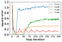
(a) $\Delta T=5$

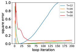
(b) $\Delta T=10$

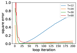
(c) $\Delta T=15$

Figure 4: The validation error of trained models, evaluated on regression with representation task, with varying hyperparameters $T$ and $\Delta T$. The AlgoFormers are trained for $T$ loops, defined in Equation (6), and the evaluation focuses on square loss at longer iterations, where the number of loop iterations far exceeds $T$.

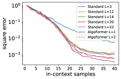
(a) Varying numbers of layers

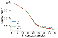
(b) Varying numbers of heads

Figure 5: The validation error of trained models, evaluated on regression with representation task, with varying numbers of layers (denoted as $L$) and heads (denoted as $h$). In the context of AlgoFormer, the number of layers $L$ corresponds to the layers in the pre-, looped, and post-transformers, all of which are $L$-layer transformers. The AlgoFormers are trained with $(T,\Delta T)=(20,15)$, defined in Equation (6).

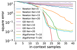
(a) Linear regression, $\sigma=0$

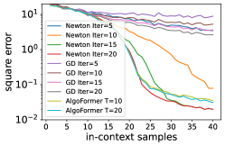
(b) Linear regression, $\sigma=0.1$

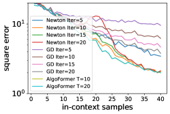
(c) Linear regression, $\sigma=1.0$

Figure 6: The validation error of trained AlgoFormer models and the linear regression models optimized by gradient descent and Newton’s method (with different iteration steps). The AlgoFormers are trained with $(T,\Delta T)=(20,15)$ and $(T,\Delta T)=(10,10)$, defined in Equation (6). Here, Newton and GD denote the Newton’s method in Equation (4) and classical gradient descent, respectively.

Loop iterations. We conduct comprehensive experiments on the AlgoFormer with varying loop numbers, on solving the regression with representation task. The results highlight the crucial role of both $T$ and $\Delta T$ in the performance of the AlgoFormer. It is observed that a larger $\Delta T$ contributes to the stable inference of transformers. Comparing Figure 4a with Figures 4b and 4c, it is evident that a larger $\Delta T$ enhances stable long-term inference. The number of loop iterations $T$ determines the model capacity in expressing algorithms. However, it is important to note that there exists a trade-off between the iteration numbers $(T,\Delta T)$ and computational costs. Larger $(T,\Delta T)$ certainly increases model capacity but also leads to higher computational costs and challenges in model training, as reflected in Figure 4.

Number of heads and layers. In our experiments on the AlgoFormer, we vary the numbers of heads and layers in $\text{TF}_{\text{loop}}$ while addressing the regression with representation task. The results reveal a consistent trend that an increase in both the number of heads and layers leads to lower errors. This aligns with our intuitive understanding, as transformers with greater numbers of heads and layers exhibit enhanced expressiveness. However, a noteworthy observation is that 4-layer and 16-head transformers may exhibit suboptimal performance, possibly due to increased optimization challenges during model training. This finding underscores the importance of carefully selecting the model size, as a larger model, while offering higher expressiveness, may present additional training difficulties. The visualized results are shown in Figure 5. Moreover, compared with the standard transformer (GPT-2), even with the same number of layers, the AlgoFormer exhibits better performance, mainly due to the introduced algorithmic structure. This finding highlights the role of the regularization of model structure. Therefore, we have reasons to believe that the good performance of the AlgoFormer not only comes from the higher expressiveness with deeper layers but also from the regularization of model architecture, which facilitates easier training and good generalization.

B.3 Comparison with Newton’s Method and Gradient Descent

In this subsection, we compare the AlgoFormer with Newton’s method and gradient descent in solving linear regression problems. We adopt the same default hyperparameters as specified in Appendix B.1.

As illustrated in Figure 6, we observe that in the noiseless case, the AlgoFormer outperforms both Newton’s method and gradient descent in the beginning stages. However, Newton’s method suddenly achieves nearly zero loss ( machine precision) later on, benefiting from its superlinear convergence. In contrast, our method maintains an error level around $1e-3$. With increasing noise levels, both Newton’s method and gradient descent converge slowly, while our method exhibits better performance.

Several aspects contribute to this phenomenon. Firstly, in the noiseless case, Newton’s method can precisely recover the weights through the linear regression objective in Equation (5), capitalizing on its superlinear convergence. On the other hand, the AlgoFormer operates as a black-box, trained from finite data. While we demonstrate good model expressiveness, the final generalization error of the trained transformer results from the model’s expressiveness, the finite number of training samples, and the optimization error. Despite exhibiting high expressiveness, the trained AlgoFormer cannot eliminate the last two errors entirely. This observation resonates with similar findings in solving partial differential equations (Raissi et al., 2019) and large linear systems (Gu & Ng, 2023) using deep learning models.

Secondly, with larger noise levels, Newton’s method shows suboptimal results. This is partly due to the inclusion of noise, which slows down the convergence rate, and Newton’s method experiences convergence challenges when moving away from the local solution. In terms of global convergence, the transformer demonstrates superior performance compared to Newton’s method.

In conclusion, although the transformer may be smarter than human-designed algorithms (Newton’s method and gradient descent), it currently cannot replace these classical algorithms in specific scientific computing tasks. Human-designed algorithms, backed by problem priors and precise computation, achieve irreplaceable performance. It’s important to note that deep learning models, including transformers, are specifically designed for solving black-box tasks where there is limited prior knowledge but sufficient observation samples. We expect that transformers, with their substantial expressiveness, hold the potential to contribute to designing implicit algorithms in solving scientific computing tasks.

References

- Ahn et al. (2023) Ahn, K., Cheng, X., Daneshmand, H., and Sra, S. Transformers learn to implement preconditioned gradient descent for in-context learning. Advances in Neural Information Processing Systems, 2023. URL https://openreview.net/forum?id=LziniAXEI9.
- Akyürek et al. (2023) Akyürek, E., Schuurmans, D., Andreas, J., Ma, T., and Zhou, D. What learning algorithm is in-context learning? investigations with linear models. In International Conference on Learning Representations, 2023. URL https://openreview.net/forum?id=0g0X4H8yN4I.
- Bai et al. (2023) Bai, Y., Chen, F., Wang, H., Xiong, C., and Mei, S. Transformers as statisticians: Provable in-context learning with in-context algorithm selection. Advances in Neural Information Processing Systems, 2023. URL https://openreview.net/forum?id=liMSqUuVg9.
- Brown et al. (2020) Brown, T., Mann, B., Ryder, N., Subbiah, M., Kaplan, J. D., Dhariwal, P., Neelakantan, A., Shyam, P., Sastry, G., Askell, A., et al. Language models are few-shot learners. Advances in Neural Information Processing Systems, 33:1877–1901, 2020. URL https://proceedings.neurips.cc/paper_files/paper/2020/file/1457c0d6bfcb4967418bfb8ac142f64a-Paper.pdf.
- Cao (2021) Cao, S. Choose a transformer: Fourier or galerkin. Advances in Neural Information Processing Systems, 34:24924–24940, 2021. URL https://proceedings.neurips.cc/paper/2021/hash/d0921d442ee91b896ad95059d13df618-Abstract.html.
- Devlin et al. (2019) Devlin, J., Chang, M.-W., Lee, K., and Toutanova, K. Bert: Pre-training of deep bidirectional transformers for language understanding. Proceedings of the 2019 Conference of the North American Chapter of the Association for Computational Linguistics: Human Language Technologies, 1:4171–4186, 2019. URL https://aclanthology.org/N19-1423.
- Dosovitskiy et al. (2021) Dosovitskiy, A., Beyer, L., Kolesnikov, A., Weissenborn, D., Zhai, X., Unterthiner, T., Dehghani, M., Minderer, M., Heigold, G., Gelly, S., Uszkoreit, J., and Houlsby, N. An image is worth 16x16 words: Transformers for image recognition at scale. In International Conference on Learning Representations, 2021. URL https://openreview.net/forum?id=YicbFdNTTy.
- Edelman et al. (2022) Edelman, B. L., Goel, S., Kakade, S., and Zhang, C. Inductive biases and variable creation in self-attention mechanisms. In International Conference on Machine Learning, pp. 5793–5831. PMLR, 2022. URL https://proceedings.mlr.press/v162/edelman22a.html.
- Feng et al. (2023) Feng, G., Gu, Y., Zhang, B., Ye, H., He, D., and Wang, L. Towards revealing the mystery behind chain of thought: a theoretical perspective. Advances in Neural Information Processing Systems, 2023. URL https://openreview.net/forum?id=qHrADgAdYu.
- Finn et al. (2017) Finn, C., Abbeel, P., and Levine, S. Model-agnostic meta-learning for fast adaptation of deep networks. In International Conference on Machine Learning, pp. 1126–1135. PMLR, 2017. URL https://proceedings.mlr.press/v70/finn17a.html.
- Fu et al. (2023) Fu, D., Chen, T.-Q., Jia, R., and Sharan, V. Transformers learn higher-order optimization methods for in-context learning: A study with linear models. arXiv preprint arXiv:2310.17086, 2023.
- Garg et al. (2022) Garg, S., Tsipras, D., Liang, P. S., and Valiant, G. What can transformers learn in-context? a case study of simple function classes. Advances in Neural Information Processing Systems, 35:30583–30598, 2022. URL https://openreview.net/forum?id=flNZJ2eOet.
- Giannou et al. (2023) Giannou, A., Rajput, S., Sohn, J.-Y., Lee, K., Lee, J. D., and Papailiopoulos, D. Looped transformers as programmable computers. In International Conference on Machine Learning, volume 202, pp. 11398–11442. PMLR, 2023. URL https://proceedings.mlr.press/v202/giannou23a.html.
- Gu & Ng (2023) Gu, Y. and Ng, M. K. Deep neural networks for solving large linear systems arising from high-dimensional problems. SIAM Journal on Scientific Computing, 45(5):A2356–A2381, 2023.
- Guo et al. (2024) Guo, T., Hu, W., Mei, S., Wang, H., Xiong, C., Savarese, S., and Bai, Y. How do transformers learn in-context beyond simple functions? a case study on learning with representations. International Conference on Learning Representations, 2024. URL https://openreview.net/forum?id=ikwEDva1JZ.
- Gurevych et al. (2022) Gurevych, I., Kohler, M., and Şahin, G. G. On the rate of convergence of a classifier based on a transformer encoder. IEEE Transactions on Information Theory, 68(12):8139–8155, 2022.
- Huang et al. (2023) Huang, Y., Cheng, Y., and Liang, Y. In-context convergence of transformers. arXiv preprint arXiv:2310.05249, 2023.
- Imani et al. (2023) Imani, S., Du, L., and Shrivastava, H. MathPrompter: Mathematical reasoning using large language models. In Proceedings of the 61st Annual Meeting of the Association for Computational Linguistics (Volume 5: Industry Track), pp. 37–42. Association for Computational Linguistics, 2023. URL https://aclanthology.org/2023.acl-industry.4.
- Kazemnejad et al. (2023) Kazemnejad, A., Padhi, I., Ramamurthy, K. N., Das, P., and Reddy, S. The impact of positional encoding on length generalization in transformers. Advances in Neural Information Processing Systems, 2023. URL https://openreview.net/forum?id=Drrl2gcjzl.
- Krishnamoorthy et al. (2023) Krishnamoorthy, S., Mashkaria, S. M., and Grover, A. Diffusion models for black-box optimization. In International Conference on Machine Learning, volume 202, pp. 17842–17857. PMLR, 2023. URL https://proceedings.mlr.press/v202/krishnamoorthy23a.html.
- Li et al. (2019) Li, S., Jin, X., Xuan, Y., Zhou, X., Chen, W., Wang, Y.-X., and Yan, X. Enhancing the locality and breaking the memory bottleneck of transformer on time series forecasting. Advances in Neural Information Processing Systems, 32, 2019. URL https://papers.neurips.cc/paper_files/paper/2019/hash/6775a0635c302542da2c32aa19d86be0-Abstract.html.
- Li et al. (2023) Li, Y., Sreenivasan, K., Giannou, A., Papailiopoulos, D., and Oymak, S. Dissecting chain-of-thought: Compositionality through in-context filtering and learning. In Advances in Neural Information Processing Systems, 2023. URL https://openreview.net/forum?id=xEhKwsqxMa.
- Li et al. (2017) Li, Z., Zhou, F., Chen, F., and Li, H. Meta-sgd: Learning to learn quickly for few-shot learning. arXiv preprint arXiv:1707.09835, 2017.
- Mahankali et al. (2024) Mahankali, A., Hashimoto, T. B., and Ma, T. One step of gradient descent is provably the optimal in-context learner with one layer of linear self-attention. International Conference on Learning Representations, 2024. URL https://openreview.net/forum?id=8p3fu56lKc.
- Ontanon et al. (2022) Ontanon, S., Ainslie, J., Fisher, Z., and Cvicek, V. Making transformers solve compositional tasks. In Proceedings of the 60th Annual Meeting of the Association for Computational Linguistics (Volume 1: Long Papers), pp. 3591–3607, 2022. URL https://aclanthology.org/2022.acl-long.251.
- Pan & Schreiber (1991) Pan, V. and Schreiber, R. An improved newton iteration for the generalized inverse of a matrix, with applications. SIAM Journal on Scientific and Statistical Computing, 12(5):1109–1130, 1991.
- Peebles et al. (2022) Peebles, W., Radosavovic, I., Brooks, T., Efros, A. A., and Malik, J. Learning to learn with generative models of neural network checkpoints. arXiv preprint arXiv:2209.12892, 2022.
- Press et al. (2022) Press, O., Smith, N., and Lewis, M. Train short, test long: Attention with linear biases enables input length extrapolation. In International Conference on Learning Representations, 2022. URL https://openreview.net/forum?id=R8sQPpGCv0.
- Radford et al. (2019) Radford, A., Wu, J., Child, R., Luan, D., Amodei, D., Sutskever, I., et al. Language models are unsupervised multitask learners. OpenAI blog, 1(8):9, 2019.
- Raffel et al. (2020) Raffel, C., Shazeer, N., Roberts, A., Lee, K., Narang, S., Matena, M., Zhou, Y., Li, W., and Liu, P. J. Exploring the limits of transfer learning with a unified text-to-text transformer. Journal of Machine Learning Research, 21(1):5485–5551, 2020. URL https://jmlr.org/papers/volume21/20-074/20-074.pdf.
- Raissi et al. (2019) Raissi, M., Perdikaris, P., and Karniadakis, G. E. Physics-informed neural networks: A deep learning framework for solving forward and inverse problems involving nonlinear partial differential equations. Journal of Computational Physics, 378:686–707, 2019.
- Söderström & Stewart (1974) Söderström, T. and Stewart, G. On the numerical properties of an iterative method for computing the moore–penrose generalized inverse. SIAM Journal on Numerical Analysis, 11(1):61–74, 1974.
- Sohl-Dickstein et al. (2015) Sohl-Dickstein, J., Weiss, E., Maheswaranathan, N., and Ganguli, S. Deep unsupervised learning using nonequilibrium thermodynamics. In International Conference on Machine Learning, pp. 2256–2265. PMLR, 2015. URL https://proceedings.mlr.press/v37/sohl-dickstein15.html.
- Sun et al. (2023) Sun, J., Zheng, C., Xie, E., Liu, Z., Chu, R., Qiu, J., Xu, J., Ding, M., Li, H., Geng, M., et al. A survey of reasoning with foundation models. arXiv preprint arXiv:2312.11562, 2023.
- Takakura & Suzuki (2023) Takakura, S. and Suzuki, T. Approximation and estimation ability of transformers for sequence-to-sequence functions with infinite dimensional input. In International Conference on Machine Learning, volume 202, pp. 33416–33447. PMLR, 2023. URL https://proceedings.mlr.press/v202/takakura23a.html.
- Vaswani et al. (2017) Vaswani, A., Shazeer, N., Parmar, N., Uszkoreit, J., Jones, L., Gomez, A. N., Kaiser, Ł., and Polosukhin, I. Attention is all you need. Advances in Neural Information Processing Systems, 30, 2017. URL https://proceedings.neurips.cc/paper_files/paper/2017/hash/3f5ee243547dee91fbd053c1c4a845aa-Abstract.html.
- Von Oswald et al. (2023) Von Oswald, J., Niklasson, E., Randazzo, E., Sacramento, J., Mordvintsev, A., Zhmoginov, A., and Vladymyrov, M. Transformers learn in-context by gradient descent. In International Conference on Machine Learning, pp. 35151–35174. PMLR, 2023. URL https://proceedings.mlr.press/v202/von-oswald23a.html.
- Wei et al. (2022) Wei, J., Wang, X., Schuurmans, D., Bosma, M., Xia, F., Chi, E., Le, Q. V., Zhou, D., et al. Chain-of-thought prompting elicits reasoning in large language models. Advances in Neural Information Processing Systems, 35:24824–24837, 2022. URL https://openreview.net/forum?id=_VjQlMeSB_J.
- Yang et al. (2024) Yang, L., Lee, K., Nowak, R. D., and Papailiopoulos, D. Looped transformers are better at learning learning algorithms. In International Conference on Learning Representations, 2024. URL https://openreview.net/forum?id=HHbRxoDTxE.
- Yu et al. (2024) Yu, L., Jiang, W., Shi, H., Yu, J., Liu, Z., Zhang, Y., Kwok, J. T., Li, Z., Weller, A., and Liu, W. Metamath: Bootstrap your own mathematical questions for large language models. International Conference on Learning Representations, 2024. URL https://openreview.net/forum?id=N8N0hgNDRt.
- Zhang et al. (2023a) Zhang, R., Frei, S., and Bartlett, P. L. Trained transformers learn linear models in-context. arXiv preprint arXiv:2306.09927, 2023a.
- Zhang et al. (2023b) Zhang, S., Fan, R., Liu, Y., Chen, S., Liu, Q., and Zeng, W. Applications of transformer-based language models in bioinformatics: a survey. Bioinformatics Advances, 3(1):vbad001, 2023b.
- Zheng et al. (2023) Zheng, C., Liu, Z., Xie, E., Li, Z., and Li, Y. Progressive-hint prompting improves reasoning in large language models. arXiv preprint arXiv:2304.09797, 2023.