Capillary levelling of thin liquid films of power-law rheology
Abstract
We find solutions that describe the levelling of a thin fluid film coating a substrate, comprising a non-Newtonian power law fluid, under the influence of surface tension. We consider the evolution from both periodic and localised initial conditions. These solutions exhibit the generic property that the profiles are weakly singular (that is, higher order derivatives do not exist), at points where the pressure gradient vanishes. Numerical solutions of the thin film equation are shown to approach one of the two cases for appropriate initial conditions.
1 Introduction
The importance of free-surface lubrication or coating flows to industry and science is well documented [Craster2009, Oron1997, Weinstein2004]. Examples of applications include the construction of smooth, or deliberately patterned, surfaces, describing the evolution of lava flows and ice sheets, among others. The mathematical modelling of such phenomena using the lubrication approximation, which allows the full governing partial differential equations and boundary conditions to be collapsed to a single equation for the film thickness, is also ubiquitous [Craster2009, Oron1997].
For small scale industrial applications in which surface tension is a dominant effect, fluids are frequently better modelled using a non-Newtonian, rather than Newtonian, rheological model. A very popular model is the power-law model:
| (1) |
where is the stress tensor, is the strain rate tensor, is the power law rheology exponent, and is a constant of proportionality (see [Myers2005] for a discussion of different rheological models). The Newtonian case is recovered when , in which case is the fluid viscosity. When , the effective viscosity is decreasing in the strain rate, while for , it is increasing. These two cases are thus known as shear-thinning and shear-thickening, respectively. Shear thinning fluids are more common in practice. The importance of rheology in the coating industry is described in [Eley2005].
From a mathematical perspective, the evolution of a lubricating film, comprising a power law fluid, under the effect of surface tension, has been considered with a focus on droplet spreading [King2001], or inclined or vertical substrates [Allouche2015, Balmforth2003, Sylvester1973]. The competition between surface tension and other effects such as van der Waals disjoining pressure, [Garg2017], and horizontally induced thermocapillary stress [Mantripragada2022].
In this article we focus on the deceptively simple problem that is the levelling of a film due to surface tension, in which a perturbed uniform film tends to flatten out over time. In the Newtonian case, this phenomenon has been studied in the context of viscometry [Benzaquen2013, Benzaquen2014, McGraw2011, McGraw2012]; by measuring the evolution of a perturbed film over time, the viscosity of the fluid may be determined. In these works, explicit similarity solutions are found that model the levelling process. This same application in the power-law fluid case has been studied to a lesser extent; [Iyer1996] perform numerical calculations of the levelling problem with a Carreau fluid and compare to experimental results. [Ahmed2015] perform a purely numerical study on power law fluids. The similarity solutions considered in the present study are also a case of nonlinear differential equations whose existence is established in [Bernis1991]. However, the explicit computation of similarity solutions that govern levelling behaviour, and comparison with numerical solutions, has not previously been undertaken in for power-law rheology.
Suitably nondimensionalised, the equation for a thin film of thickness and rheology (1) evolving purely due to surface tension in one dimension is [Garg2017, King2001]:
| (2) |
where we have explicitly defined the flux . Here is the power law exponent in the rheology; , and correspond to the shear thinning, Newtonian, and shear thickening cases, respectively. In the derivation of (2), the third derivative arises as the gradient of the Laplace pressure (the interface curvature being given by the second derivative in the lubrication approximation).
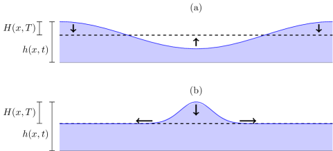
The governing equation (2) has as an exact solution a perfectly uniform film which can be taken to be identically (we are free in the nondimensionalisation to specify the characteristic thickness as the vertical length scale). In this work we consider the evolution of perturbations of this uniform film, distinguishing two cases: the evolution of a perturbation that is periodic in space, which is equivalent to a perturbation over an entire finite domain with no-flux boundary conditions; and the evolution of an initially localised perturbation in an infinite spatial domain (see Fig. 1). These two cases generalise the results of a Newtonian liquid film, which are modal linear stability of a flat interface, and the similarity solution derived in [Benzaquen2013, Benzaquen2014], respectively. We numerically determine the similarity solutions that describe each of these in the non-Newtonian case. The computed solutions demonstrate a general property of solutions to power-law thin film equations, namely, the non-existence of higher derivatives (depending on the exponent ). As well as of mathematical interest, this property is important to establish from a modelling perspective, as it affects the accuracy and potentially the correctness of numerical schemes. We also carry out numerical simulations of the fully time-dependent thin film equation, and show that solutions with more general initial conditions are attracted to the periodic or similarity solutions as appropriate.
2 Weakly singular nature and levelling solutions
2.1 Weakly singular nature
In the Newtonian case, (2) is degenerate in that the flux vanishes at points where the thickness vanishes. In the non-Newtonian case, (2) is degenerate even if is not zero, at a point where the pressure gradient (that is, the third derivative of ) is zero. A sensible expansion for near such a point is
where is an as-yet unknown power. On substitution into (2), the leading order term in the flux is
so that
Generally at such a point, thus, we thus require . For non-integer , we expect the film profile will be weakly singular, such that is times differentiable. This is particular important for shear-thinning flows () as then we only expect weak, rather than classical, solutions of the fourth order equation (2) to exist. We will observe this singular behaviour in each of the solutions constructed in this article. We note that as special cases, if , then a singularity at higher order will occur as the gradient of flux must balance with another term, while if is an integer not equal to unity, then there will be higher order noninteger powers in the flux that need to be balanced, requiring higher order non-integer powers in the expansion of . We do not consider these special cases further here.
2.2 Close-to-uniform approximation
We examine the behaviour of a film that is close to the uniform solution by writing
| (3) |
where . Then to ,
| (4) |
In the Newtonian case (), (4) is linear, and no time rescaling is necessary, but in the non-Newtonian case (), (4) remains nonlinear, and the amplitude-dependent scaling in time is necessary for the two terms in the equation to be in balance. The near-level approximation (4) has the same property of the original equation (2), in that must be weakly singular at any point where the third spatial derivative is zero in order for the evolution to be well defined.
We now construct two special classes of solutions to (4), generalising the known results for the Newtonian case (see Fig. 1). Firstly, we consider solutions periodic in , which are relevant for initial conditions that are periodic or on bounded domains with no-flux conditions. Secondly, we construct similarity solutions that are appropriate for initial conditions that are spatially localised.
2.3 Periodic initial condition
We start with solutions that are periodic in . In the Newtonian case () this is equivalent to computing the linear stability of the uniform solution. For a given wavenumber (so that the period is ) we have
where the amplitude is arbitrary (equivalent to time-translational invariance). For , the near-level behaviour is essentially nonlinear, and linear stability approaches are not appropriate. Instead, we assume a solution of (4) more generally in which the time and space dependence may be separated, or, equivalently, a similarity solution in which the spatial scale remains fixed. The appropriate ansatz depends on whether the fluid is shear thinning or thickening:
| (5) |
where is a periodic, but as yet undetermined, function (the -dependent constant is included to simplify the problem for ). The above ansatz represents infinite-time but algebraic decay for the shear thinning () case, and finite-time (at ) levelling for the shear thickening case; of course, the solutions are invariant to translations in time, and the finite levelling time will depend on the initial amplitude.
Under the ansatz (5), satisfies the ordinary differential equation
for both shear-thinning and thickening. Let , then satisfies
| (6) |
with readily found from by . Since any solution to (6) may be scaled onto another solution by , , it suffices to find a solution with period , which can then be scaled to find the solution for any other period.
2.3.1 Numerical computation
Corresponding to the behaviour of the original problem near a singular point described in Section 2.1 for noninteger , solutions to (6) will be weakly singular at points where , with an expansion of the form
In the shear-thinning case, will thus be four (but not five)-times differentiable, corresponding to the profile (and so the time-dependent profile ) being three but not four-times differentiable at points where the pressure gradient . However, since (6) is fourth order, this singularity is weak enough to be able to proceed (that is, we have essentially integrated the equation by solving for the antiderivative of ).
Assuming symmetry, we find the solution on the half period with the conditions
| (7) |
In the half-period, may be taken to be positive. We calculate solutions to the boundary value problem (6), (7) numerically using the MATLAB function bvp4c. An initial guess is provided close to from the asymptotic solution described below (Section 2.3.2). A continuous branch of solutions is then constructed by numerical continuation for decreasing and increasing power law exponent , using the previously computed solution as an initial guess for the next.
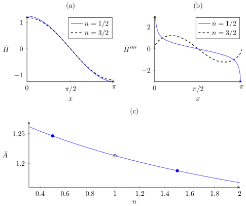
In Fig. 2 we plot the results of this computation, focussing on the values and . We include both the profiles , as well as the fourth derivative . The profiles themselves are visually difficult to distinguish from the sinusoidal profiles that are exact for the Newtonian case (), but have non-arbitrary, -dependent amplitude. In plotting the fourth derivative, the difference between the cases is stark, in particular, that the shear thinning case () is singular at the peak and trough of the periodic profile (), while for the shear-thickening case (), the fourth derivative is bounded and continuous (although the next derivative will indeed be singular). We also plot the amplitude , calculated as half of the peak to trough distance ; this value varies only weakly in the range of values calculated.
2.3.2 Close to Newtonian limit
In the above method, the starting point of the numerical solutions was found by determining the asymptotic solution to (6) in the close-to-Newtonian limit . This approximation is also of interest in itself. Defining , where :
so that if , we have
Applying the boundary conditions (7) to , we find
with the amplitude determined by a solvability condition for . Applying the same boundary conditions to , we must have that (by the Fredholm alternative)
Thus either (the trivial solution), or
| (8) |
This value agrees with the numerically computed results near (see Fig. 2). We note that in this asymptotic result we have not considered the region near where will be weakly singular, as it does not play a role in selecting the amplitude .
2.4 Localised initial condition
We now find solutions relevant for an initial condition that is localised in an infinite spatial domain. In this case, relevant solutions are similarity solutions that describe how an initial peak spreads over time.
For any value of , similarity solutions to (4), symmetric around the point , take the form
| (9) |
where are the similarity variables, is an arbitrary amplitude included so that we can specify , and the similarity exponent is determined from the two conditions that the terms in (4) have the same time dependence, and that mass is conserved. Substituting (9) into (4) results in the ordinary differential equation for similarity profiles:
subject to symmetry conditions at zero. This equation may be integrated once and the boundary conditions used to result in the third-order equation
| (10) |
A third condition is imposed by requiring solutions to decay as . Similarly to the periodic case, since we only deal with third derivatives of in (10), the singularities that are present (in particular in the fourth derivative for ) will not prevent numerical computation of the solution.
In the Newtonian case, the similarity solution has been previously identified in [Benzaquen2013, Benzaquen2014]; In this case the similarity exponent , and the equation for the profile (10) is linear:
which, given , , and decay at infinity, has exact solution in terms of hypergeometric functions:
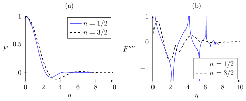
For , numerical solutions to (10) are obtained by shooting from . Since , there is one parameter that must be determined numerically by requiring that as . We use ode45 in MATLAB to solve the equation up to a sufficiently large value of , combined with a root finding method to determine the appropriate value of . The solutions so found are plotted in Fig. 3, including both the profiles and the fourth derivative, calculated from the numerical solution using
As for periodic solutions, plotting this fourth derivative shows the presence of singularities at higher order. As the similarity solution oscillates an infinite number of times as , there are an infinite sequence of such singularities.
3 Comparison with numerical simulations
In order to test the universality of the solutions found in Section 2, we simulate the time-dependent lubrication equation (2). We use a finite volume method, which naturally solves the weak formulation of a conservative transport equation. This property is particularly important in the present case as for , we do not expect (2) to have classical (four-times differentiable) solutions. We consider a domain divided into cells of width , with the th cell centre at , . The finite difference expression for the third derivative of on the face between the th and th cell is
where is taken to be the representative value of in cell , while the value of the thickness itself on the face is given by the average . These expressions are used to approximate the fluxes . The transport equation (2) then gives
No flux conditions are imposed at the two ends and , while no-slope conditions () are used to define ghost node values that allow the third derivative to be computed on all internal faces. The numerical scheme is then advanced in time using MATLAB’s ode15s implicit time-stepping algorithm.
Using this method we compute solutions of (2) for the two values of the power law exponent we have focussed on thus far ( and ), and initial conditions that test the behaviour of periodic and localised solutions, respectively. To test the behaviour of periodic solutions, we choose a domain size of and an initial condition
From the ansatz (5) we predict that the amplitude , which we calculate numerically as , will either decay algebraically or undergo finite-time levelling, depending on :
where is the (-dependent) amplitude of the solution to the profile function , and is the finite levelling time. For and , then, these become
| (11) |
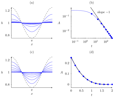
In this case, the prefactor is determined independently of the initial condition (although not of the domain size). The levelling time is initial condition-dependent, however. In Fig. 4 we show the results of the numerical simulation. The observed behaviour of the amplitudes are in agreement with the prediction (11), indicating that the levelling solutions we found in Section 2 are accurate, and are attractors of more generic initial conditions.
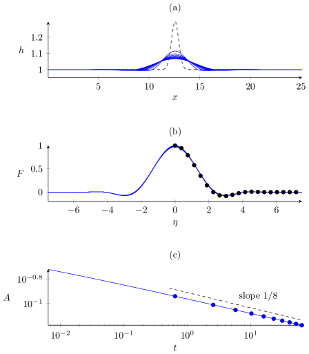
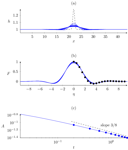
To test the behaviour of localised initial conditions, we start with a Gaussian initial condition
for both and , with domain size sufficiently large so as to avoid the boundary having an effect on the evolution. The similarity ansatz (9) predicts the amplitude, defined by , will go as
| (12) |
As is arbitrary in (9), the prefactor in this relation is dependent on initial condition. We plot the results of these simulations in Fig. 5 for , and Fig. 6 for . In each case, the profiles rapidly evolve toward the relevant similarity solution (with the appropriate value of estimated from the numerical solution at the final time), and the behaviour of the amplitude approaches the predicted power law (12). Again, the strong agreement indicates the similarity solution is an attractor for initially localised perturbations on an infinite domain.
4 Discussion
By explicitly calculating similarity solutions that describe levelling, we have determined the power-law decay of the amplitude of perturbations of a flat film. As the decay depends on the power in the rheology (1), our results imply that levelling experiments could be used to determine the rheology of fluids, in a similar way as they are used to determine the viscosity of presumed-Newtonian fluids [Benzaquen2013, Benzaquen2014].
We have also demonstrated that solutions to lubrication equations with power-law rheology will be weakly singular at points where the pressure gradient vanishes. This will be also true in more complicated models, for instance those that feature disjoining pressure, Marangoni forces, or gravity. Despite the weakly singular nature of solutions to (2), previous studies have successfully computed solutions numerically. Indeed, the distinct infinite-time and finite-time levelling, for shear-thinning and thickening fluids, respectively, can be observed in the numerical results of [Ahmed2015], although they do not interpret them as such. Numerical studies on power-law thin films are likely to numerically regularise the singularities, or be formulated in such a way that they correctly solve the weak version of the equation (as our method does). However, as the singular behaviour becomes more severe as is reduced, it is likely that it will be important to take into account for studies that wish to examine the highly shear-thinning limit (). On the other hand, studies on inclined or vertical planes, or with imposed tangent stress, may avoid this issue by never having points at which the pressure gradient vanishes.
The rheology itself may be explicitly regularised, using, for example, a Carreau-type model [Myers2005], which acts like a power law fluid except for small strain rate, where it behaves in a Newtonian manner. For more complex rheology, the flux becomes more complicated to compute, although it is possible to make progress using the method described in [Pritchard2015] (see also [Hinton2022] for the two-dimensional case). Under such a regularisation, a thin film may be expected to level in the same way as described in this paper, until the film becomes very close to level, at which point the Newtonian regime will be reached, and perturbations will switch to exponential decay according to the linear stability analysis of the Newtonian case.
Extending to two spatial dimensions is also of interest. Presumably, there exists a radially symmetric similarity solution that would describe the decay of localised perturbations. For periodic perturbations, one could imagine a radial solution for a thin film in a finite circular domain, or, for a more general shape, one would have to solve the nonlinear elliptic equation that is the counterpart to (6) in higher dimensions. The power law decay of the amplitude in time, however, would be universal.