Isotope shift analysis with the $4f^{14}6s^{2}~{}^{1}S_{0}-4f^{13}5d6s^{2}(J=2)$ transition in ytterbium

Abstract

Measurements of isotope shifts have recently been attracting considrable attentions due to their potential in searching for new forces. We report on the isotope shifts of the $4f^{14}6s^{2}~{}^{1}S_{0}-4f^{13}5d6s^{2}(J=2)$ transition at 431 nm in Yb, based on absolute frequency measurements with an accuracy of $\sim 10$ kHz. Utilizing these data, previous reports for other transitions, and theoretical calculation of electronic structure, analyses of isotope shifts on various aspects are performed, including determination of the hyperfine constants for ¹⁷³Yb, assessment of nuclear charge radii, analysis on King plots, and a search for new bosons mediating the force between an electron and a neutron. The analysis motivates further precision measurements on isotope shifts of the narrow-linewidth transitions in ytterbium, not only for the bosonic isotopes but also for the fermionic isotopes.

I Introduction

Isotopes, which differs in the number of neutrons $N$ in the nucleus within the same element, exhibit slightly varied physical properties. Such properties include macroscopic quantities, e.g., phase transition temperatures, reaction rates of chemical reactions, and diffusion constants, as well as nuclear properties specific to nuclei. The nuclear properties manifest themselves particularly well in the difference in the resonant frequency $\nu$ for a transition $\alpha$, which is called an isotope shift. Typically ranging from 100 MHz to 1 GHz, the isotope shift for an optical transition of $\sim 100$ THz is easily observed with laser spectroscopies.

Isotope shifts are conventionally attributed primarily to two sources. One is the mass difference between nuclei changing the reduced mass and correlation of electrons, which is called the mass shift. The other is the variation of the nuclear charge radii distorting the Coulomb potential inside the nucleus, referred to as the field shift. Precisely determining the amount of isotope shifts can potentially serve as a good probe of nuclear structure.

In addition to these two main factors, recent development in analysis of isotope shifts incorporates higher order terms as shown in the following equation [1].

$$\nu_{\alpha}^{AA^{\prime}}= F_{\alpha}\langle r^{2}\rangle^{AA^{\prime}}+K_{\alpha}\mu^{AA^{\prime}}+G_{\alpha}^{(4)}\langle r^{4}\rangle^{AA^{\prime}}$$ (1)

$$+G_{\alpha}^{(2)}[(\langle r^{2}\rangle^{A^{\prime\prime}})^{2}]^{AA^{\prime}}+v_{ne}D_{\alpha}N^{AA^{\prime}}$$

Here, the superscripted mass number $A$ specifies the isotope, and $X^{AA^{\prime}}\equiv X^{A}-X^{A^{\prime}}$. _α denotes the transition. Note that in this paper transitions are labeled with their wavelengths (three-digit number in the unit of nm), and all transitions of ytterbium appearing in this paper are summarized in Table 1. Coefficients $F_{\alpha}$ and $K_{\alpha}$ characterize the field shift and mass shift, respectively. $\langle r^{n}\rangle$ is the $n$th moment of the nuclear charge. $\mu^{A}=1/m^{A}$ is the inverse mass. The third and fourth terms are the quadratic field shift, where $[(\langle r^{2}\rangle^{A^{\prime\prime}})^{2}]^{AA^{\prime}}=(\langle r^{2}\rangle^{AA^{\prime\prime}})^{2}-(\langle r^{2}\rangle^{A^{\prime}A^{\prime\prime}})^{2}$, and the fourth-moment shift, respectively. The fifth term shows the effect of a Yukawa potential $V_{ne}=\hbar cv_{ne}\exp(-m_{\phi}cr/\hbar)/r$ on the electrons besides the Coulomb potential. $v_{ne}=(-1)^{s+1}y_{n}y_{e}/(4\pi\hbar c)$ characterizes a hypothetical new force between a neutron and an electron, where $s$ is the spin of the boson mediating this force, $y_{n,e}$ are coupling constants to a neutron and an electron, and $m_{\phi}$ is the mass of the boson.

The field shift term can be eliminated by a set of isotope shifts for another transition $\beta$. The resulting equation is

$$\frac{\nu_{\beta}^{AA^{\prime}}}{\mu^{AA^{\prime}}} = \frac{F_{\beta}}{F_{\alpha}}\frac{\nu_{\alpha}^{AA^{\prime}}}{\mu^{AA^{\prime}}}+K_{\beta,\alpha}+\frac{\langle r^{4}\rangle^{AA^{\prime}}}{\mu^{AA^{\prime}}}G_{\beta,\alpha}^{(4)}$$ (2)

$$+\frac{[(\langle r^{2}\rangle^{A^{\prime\prime}})^{2}]^{AA^{\prime}}}{\mu^{AA^{\prime}}}G_{\beta,\alpha}^{(2)}+\frac{v_{ne}N^{AA^{\prime}}}{\mu^{AA^{\prime}}}D_{\beta,\alpha},$$

where $X_{\beta,\alpha}=X_{\beta}-X_{\alpha}F_{\beta}/F_{\alpha}$ for $X\in\{K,D,G^{(4)},G^{(4)}\}$. The plot between $\nu_{\beta}^{AA^{\prime}}/\mu^{AA^{\prime}}$ and $\nu_{\alpha}^{AA^{\prime}}/\mu^{AA^{\prime}}$ is called King plot and approximately linear [2], as the first two terms in the right hand are major. The breakdown of the linearity is proposed to be used for searches for the new bosons [3, 4, 5], and some advanced analysis techniques are also reported to reduce the effects with large uncertainties [6, 7], along with assessments of which higher order effects are significant [8, 9, 10, 11, 12]. For heavy atoms, normalizing both sides with $\nu_{\alpha}^{AA^{\prime}}/\mu^{AA^{\prime}}$ suppresses the influence of the uncertainty in mass [7]:

$$\frac{\nu_{\beta}^{AA^{\prime}}}{\nu_{\alpha}^{AA^{\prime}}} = \frac{F_{\beta}}{F_{\alpha}}+K_{\beta,\alpha}\frac{\mu^{AA^{\prime}}}{\nu_{\alpha}^{AA^{\prime}}}+\frac{\langle r^{4}\rangle^{AA^{\prime}}}{\nu_{\alpha}^{AA^{\prime}}}G_{\beta,\alpha}^{(4)}$$ (3)

$$+\frac{[(\langle r^{2}\rangle^{xA^{\prime\prime}})^{2}]^{AA^{\prime}}}{\nu_{\alpha}^{AA^{\prime}}}G_{\beta,\alpha}^{(2)}+\frac{v_{ne}N^{AA^{\prime}}}{\nu_{\alpha}^{AA^{\prime}}}D_{\beta,\alpha}$$

Among various experimental reports on the isotope shift measurements aimed at searching for new bosons [13, 14, 15, 16], ytterbium (Yb) is one of the most extensively studied atomic species for this purpose, as well as nuclear structure, with the nonlinearity of the King plot [7, 1, 17, 18]. The isotope shifts for the 411, 436, and 467 nm transitions in Yb⁺ are measured with $\gtrsim 300$ Hz accuracy. For Yb, precise isotope shift measurements for the 361 and 578 nm transitions are reported. However, these analyses so far only cover bosonic isotopes, because the nuclear spins in fermionic isotopes potentially add extra nonlinearity that can become a background in the search for new bosons. In fact, except for the 578 nm transition in Yb, no precise isotope shift measurements are available for fermionic isotopes; only broad-linewidth transitions utilized for laser cooling have the isotope shift data for the fermionic isotopes. Particularly, regarding a newly observed narrow-linewidth transition at 431 nm [19, 20], the absolute frequency is measured for only a single fermionic isotope [19], and isotope shifts are measured for only bosonic isotopes [20].

Table 1: Transitions in Yb and Yb⁺. The numbers listed in $\alpha$ are the wavelengths of the transitions in the unit of nm. The lower-energy state for all transitions are the ground state, which is $6s^{2}~{}^{1}S_{0}$ for Yb and $6s~{}^{2}S_{1/2}$ for Yb⁺. The $4f$ orbital is fully filled with 14 electrons unless otherwise specified. $\Gamma$ is the linewidth of the excited state.

Yb			Yb+
$\alpha$	excited state	$\Gamma$	$\alpha$	excited state	$\Gamma$
361	$5d6s~{}^{1}D_{2}$	24 kHz	411	$5d~{}^{2}D_{5/2}$	22 Hz
399	$6s6p~{}^{1}P_{1}$	29 MHz	436	$5d~{}^{2}D_{3/2}$	3 Hz
431	$4f^{13}5d6s(J=2)$	0.8 mHz	467	$4f^{13}6s^{2}~{}^{2}F_{7/2}$	0.5 nHz
556	$6s6p~{}^{3}P_{1}$	184 kHz
578	$6s6p~{}^{3}P_{0}$	7 mHz

In this paper, we report absolute frequencies for the 431 nm transition in ^{170,172,173,174,176}Yb. This report completes the list of isotope shifts of the 431 transition for all stable isotopes at 10 kHz level. Based on these new measurements and some previously reported isotope shifts for other transitions, hyperfine structure, nuclear charge radii, and King plot are analyzed. The king plot analysis also leads to a search for new bosons mediating additional force between a neutron and an electron. The results provide some insights on the nuclear structure for the fermionic isotopes for ytterbium, motivating the precise isotope shift measurements for other transitions.

II Experimental Measurements

The experimental setup and sequences are previously reported elsewhere [19]. To summarize briefly, $\sim 10^{5}$ atoms at $\sim 30$ $\upmu$K are prepared in a magneto-optical trap (MOT) formed with the 556 nm transition. Atoms are then interrogated by 431 nm probe light at 10 mW power generated by second harmonics generation from the 862 nm light emitted by a titanium-sapphire laser. The frequency of the 862 nm light is stabilized to a ultralow-expansion cavity through a frequency comb and a 1064 nm laser, with all relevant radiofrequency signals referenced to the 10 MHz clock signal supplied from a physical realization of Coordinated Universal Time maintained by the National Metrology Institute of Japan. The 431 nm probe light is retroreflected, so that the atoms are immune to the Doppler shift.

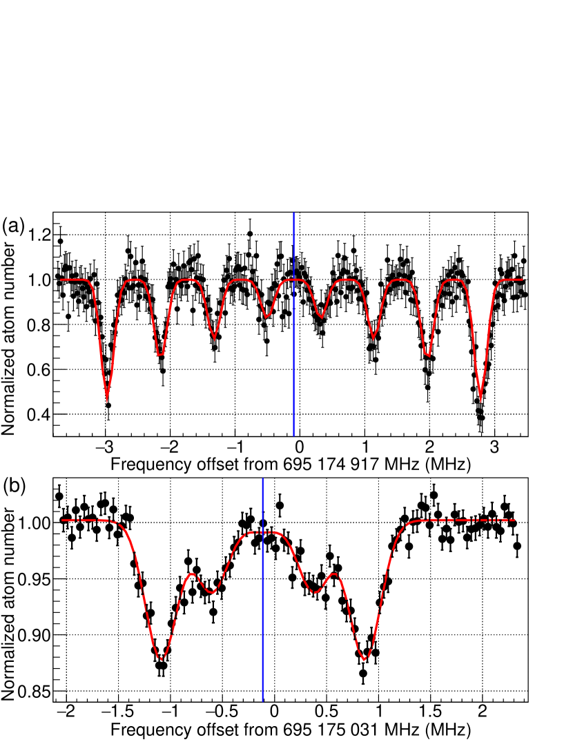
Figure 1: Spectra of the depletion of the MOT due to the 431 nm transition: (a) the $F=7/2$ hyperfine state in ¹⁷³Yb with 0.0866(13) mT bias magnetic field applied along the 431 nm probe beam. (b) ¹⁷⁴Yb. Black points show the experimental data, and the red curve is the fit of the datapoints. The blue vertical line is the average frequency obtained from the fit. See the main text for the form of the fit function.

The search for the transition is first performed for each isotope by chirping the frequency of the 431 nm light while it is irradiated to the atoms in the MOT. The chirp rate varies from 200 kHz/s to 2 MHz/s depending on the expected strength of the transition. Once the initial signal of the transition is observed, further precise measurements of the resonant frequency is performed with the frequency of the 431 nm light fixed within a cycle. For the $F=7/2,~{}5/2$, and $3/2$ hyperfine states in ¹⁷³Yb, the cycle of activating the 431 nm probe light for 3 ms while the MOT is turned off for a short preiod is repeated over 45 times. For other hyperfine states in ¹⁷³Yb and bosonic isotopes, the 431 nm light is continuously irradiated onto atoms for 1 s without turning off the MOT. In both cases, the number of atoms after the irradiation of the 431 nm light normalized by the initial atom number is estimated from the amount of fluorescence from the MOT. Every time atoms are removed and then reloaded to the MOT, the frequency of the 431 nm light is shifted to obtain the spectrum of normalized atom number $R$.

Fig. 1 (a) and (b) show sample spectra for the $F=7/2$ state in ¹⁷³Yb and ¹⁷⁴Yb, respectively. For the $F=7/2$ state in ¹⁷³Yb, distinct separation of Zeeman sublevels is observed due to a bias magnetic field of 0.0866(13) mT applied only when the MOT is deactivated, whereas the Zeeman sublevels in the ¹⁷⁴Yb spectrum overlap because of the inability of applying arbitrary bias magnetic field with the MOT active. The spectra are fitted with the following equation.

$$R=R_{0}-\sum_{i=-F}^{F}A_{|i|}\exp\left[-\frac{\left(\nu-\left(\nu_{0}+i\Delta\nu\right)\right)^{2}}{2\sigma^{2}}\right],$$ (4)

where $R_{0}$ is a constant and $\sigma$ is the width for the Gaussian. The average frequency $\nu_{0}$ is regarded as the resonant frequency for the transition, and the amount of splitting $\Delta\nu$ is induced by the Zeeman shift.

The absolute frequency of the transition is calculated by compensating systematic shifts from $\nu_{0}$. Major sources are the AC Stark shift due to the 431 nm probe beam and the Doppler shift. The former is estimated for ¹⁷³Yb and the bosonic isotopes separately, due to the potential shift in the relative position between the MOT and the probe beam. The frequency shift per 1 mW probe beam is estimated to be 2.40(1.20) kHz and 0.83(1.41) kHz for ¹⁷³Yb and ¹⁷⁴Yb as the representative of the bosonic isotopes, respectively. The Doppler shift is assumed to be zero, because the probe beam is retroreflected. However, the 3.8 kHz offset between the average of the recoil-free doublet and the bottom of the Doppler-broadened dip is added in the uncertainty [19]. For the bosonic isotopes, the frequency shift of 101.8(7.8) kHz due to the MOT is also taken into account, as estimated in Ref. [19].

Obtained absolute frequencies are summarized in Table 2. As for ¹⁶⁸Yb, which cannot be trapped with large enough number in the current setup, the absolute frequency is calculated from that for ¹⁷⁴Yb and the isotope shift reported in Ref. [20]. Differences of the absolute frequencies between bosonic isotopes reported in this work agree well within the uncertainty with the isotope shifts reported in Ref. [20].

For the $F=7/2$, $5/2$, and $3/2$ states in ¹⁷³Yb, the Landé’s $g$ factor is measured by applying bias magnetic field along the direction of the incident probe beam (See Appendix for details). The bias magnetic field is calibrated using the Zeeman splitting of the 556 nm transition with a relative uncertainty of 1.5%. The obtained $g$ factors are $g_{F}=0.662(46)$, $0.546(24)$, $0.196(24)$ for $F=7/2$, $5/2$, and $3/2$, respectively. $g_{J}$ obtained by the weighted average of these $g_{F}$ is $1.583(56)$, which is consistent with the value in Ref. [19] within an uncertainty, but is off from theoretically expected $g_{J}=1.5$ and the value in Ref. [20].

Table 2: Absolute frequencies for the 431 transition in Yb isotopes: Regarding ¹⁷¹Yb and ¹⁷³Yb, the measured quantities are the transition frequencies for each $F$ state. The number listed in the line without $F$ represents the center of gravity of all $F$ states.

$A$	F	Absolute frequency [kHz]	Reference
168		695 170 466 295(17)	[20]
170		695 172 220 247(19)	this work
171		695 172 739 827(24)
	3/2	695 171 054 858.1(8.2)	[19]
	5/2	695 173 863 140(30)	[19]
172		695 173 850 275(18)	this work
173		695 174 348 875(19)
	1/2	695 175 324 560(47)	this work
	3/2	695 175 625 655(17)	this work
	5/2	695 175 702 427(13)	this work
	7/2	695 174 916 888(12)	this work
	9/2	695 172 376 487(17)	this work
174		695 175 030 891(17)	this work
176		695 176 146 678(17)	this work

III Theoretical calculation of the electronic structure

The electronic structure of Yb is numerically calculated with configuration interaction implemented in ambit [21]. For Yb, up to $n=19$ states for $s$ and $p$ orbitals and $n=14$ states for $d$ and $f$ orbitals are included in the calculation. For Yb⁺, up to $n=16$ states are incorporated for all $s$, $p$, $d$, and $f$ orbitals. Two electron excitations from states relevant to this analysis and some other excited states and one hole excitations from the $4f$ orbital are allowed. For Yb, a hole excitation from the $5s$ and $5p$ orbitals are also allowed. $F_{\alpha}$, $K_{\alpha}$, and $D_{\alpha}$ are calculated by adjusting the initial conditions to observe the resulting energy shifts of each excited state.

In the following discussion, the results for Yb are mainly used, and the quantities for Yb⁺ are calculated to test consistency with previous reports. The calculations in this work are reasonably consistent with previous reports [7, 1, 6, 22] and experimental values [23], except for $K_{\alpha}$ for Yb⁺ ions and $K_{\beta\alpha}$, as shown in Table 6 in Appendix.

IV Data Analysis

IV.1 Hyperfine Structure

From the absolute frequencies listed in Table 2, hyperfine constants are calculated. The A constant for ¹⁷¹Yb is reported in Ref. [19]. For ¹⁷³Yb, hyperfine levels are characterized by the A, B, and C hyperfine constants $A_{h}$, $B_{h}$, and $C_{h}$ corresponding to magnetic dipole, electric quadrupole, and magnetic otcupole components (see Appendix). The best fits of the absolute frequencies with and without the octupole term are summarized in Table 3. With the octupole term, the fit quality characterized by $\chi^{2}/{\rm ndf}$ improves. However, the obtained octupole moment has only a significance $1.62\sigma$, and the shift of the dipole and quadrupole constants induced by the introduction of the octupole term is within the standard deviation. Further improvement in the precision of the spectroscopy is desired to determine whether the nucleus has a finite octupole moment. In the following analysis, to be conservative, $A_{h}$ and $B_{h}$ obtained by the fit without the octupole term are used.

Table 3: Hyperfine constants for fermionic Yb isotopes in the unit of kHz: the uncertainties include the inflation by $\sqrt{\chi^{2}/{\rm ndf}}$.

		without $C^{173}_{h}$	with $C^{173}_{h}$	Ref.
171Yb	$A^{171}_{h}$	1 123 273(13)		[19]
173Yb	$A^{173}_{h}$	-309 446.1(7.0)	-309 449.1(5.5)	this work
	$B^{173}_{h}$	-1 700 631(78)	-1 700 652(60)
	$C^{173}_{h}$		7.6(4.7)
$\chi^{2}/{\rm ndf}$		12.05	6.711

The ratio of $A_{h}$ between different isotopes equals the ratio of the nuclear $g$ factors $g^{A}$. The deviation $\Delta_{A,A^{\prime}}$ defined by the following equation is referred to as hyperfine anomaly [24]:

$$\Delta_{173,171}=\frac{A_{h}^{173}/A_{h}^{171}}{g^{171}/g^{173}}-1=\frac{A_{h}^{173}/A_{h}^{171}}{(\mu_{n}^{171}/I^{171})/(\mu_{n}^{173}/I^{173})}-1,$$ (5)

where $\mu_{n}^{A}$ and $I^{A}$ are the nuclear magnetic moment and nuclear spin, and $(\mu_{n}^{171}/I^{171})/(\mu_{n}^{173}/I^{173})=-3.6305(1)$ [25, 26, 27]. The hyperfine anomaly for the 431 nm and other transitions are summarized in Table 4. $\Delta_{173,171}$ for the $4f^{13}5d6s^{2}(J=2)$ state corresponding to the 431 nm transition is finite but particularly small compared to other states in Yb, as well as anomalies in most alkali atoms [24]. Also, it is worth noting that the singlet states tend to have large anomaly.

Table 4: Hyperfine anomalies $\Delta_{171,173}$ and electric quadrupole moments $Q$ for different states in Yb: references profvide values for the A and B constants.

State	$\Delta_{171,173}/10^{-3}$	Q ($10^{-31}$ m2)	Ref.
$6s6p~{}^{1}P_{1}$	13.90(56)	4664.6(2.5)	[28]
$4f^{13}5d6s^{2}(J=2)$	-0.156(55)	404.634(27)	this work
$6s6p~{}^{3}P_{2}$	-8.96(53)	-133.066(56)	[29]
$6s6p~{}^{3}P_{1}$	-3.856(70)	333.574(35)	[30]
$6s7s~{}^{3}S_{1}$	-3.50(34)	0.047(233)	[29]
$6s5d~{}^{1}D_{2}$	-13.0(6.7)	77.0(5.0)	[31]

In the nonrelativistic limit, $A_{h}$ and $B_{h}$ are written in the following form [24].

$$A_{h} = -\frac{1}{h}\frac{16\pi}{3}\frac{\mu_{0}}{4\pi}\mu_{B}\mu_{N}\frac{2L(L+1)}{J(J+1)}g^{A}\langle r^{-3}\rangle_{nl}$$ (6)

$$B_{h} = \frac{1}{h}\frac{e^{2}}{4\pi\epsilon_{0}}\frac{2J-1}{2J+2}\langle r^{-3}\rangle_{nl}Q$$ (7)

Here, $h$ is the Planck constant, $\mu_{0}$ and $\epsilon_{0}$ are the magnetic and electric constants, $L$ and $J$ are the electronic orbital and total angular momentum, $e$ is the elementary charge, $\mu_{B}$ and $\mu_{N}$ are the Bohr and nulcear magnetons, and $\langle r^{-3}\rangle_{nl}$ is the average over the wavefunction of the electronic state $(n,l)$. The nuclear quadrupole moment $Q$ can then be calculated as

$$Q=-\frac{\epsilon_{0}\mu_{0}}{e^{2}}\mu_{B}\mu_{N}g^{A}\frac{4L(L+1)}{J(2J-1)}\frac{B_{h}}{A_{h}}$$ (8)

The obtained $Q$ are summarized in Table 4. The values differ a lot between different states, and none of them are close to the spectroscopic nuclear quadrupole moment of $Q=2.80(4)\times 10^{-28}$ m² obtained by spectroscopy of muonic ytterbium [32]. This value is consistent with $Q\sim 2.5\times 10^{-28}$ m² for ^174,176Yb obtained from nuclear scattering experiments [33]. This suggests that significant portion of the observed quadrupole moment arises from relativistic effects, which is substantially larger than those observed in alkali atoms [24, 34].

IV.2 Nuclear charge radius

With theoretically calculated $F_{\alpha}$ and $K_{\alpha}$, $\langle r^{2}\rangle^{AA^{\prime}}$ is estimated using Eq. (1). The relative uncertainty of $\langle r^{2}\rangle^{AA^{\prime}}$ caused by the uncertainty of the spectroscopy is $\sim 10^{-5}$ (see Table 7 in Appendix), and the uncertainty for the obtained $\langle r^{2}\rangle^{AA^{\prime}}$ mainly originates from that of the theoretical calculation of $F_{\alpha}$ and $K_{\alpha}$, whose amount is difficult to estimate. To determine the uncertainty for $\langle r^{2}\rangle^{AA^{\prime}}$, $\langle r^{2}\rangle^{AA^{\prime}}_{\alpha}$ is calculated with isotope shift data for $\alpha=399$ [28], $431$, $556$ [30], and $578$ [18]. The average of them is regarded as the most likely $\langle r^{2}\rangle^{AA^{\prime}}$, and standard deviation of them is regarded as the uncertainty.

Obtained $\langle r^{2}\rangle^{AA^{\prime}}$ is plotted in Fig. 2. The values derived from the 431 nm transition result in this work are plotted together with the average values. These values tend to be smaller than the numbers in some previous reports [35, 32, 36], and closer to those in Ref. [26, 22]. The charge radii for Yb isotopes are also measured by scattering experiments with electrons [37, 38, 39] and protons [33]. Ref. [33] explicitly shows $\langle r^{2}\rangle$ for ¹⁷⁴Yb and ¹⁷⁶Yb estimated by proton scattering. Refs. [37, 38] provide experimental values of $\langle r^{2}\rangle^{A}$ for ¹⁷⁴Yb and ¹⁷⁶Yb from electron scattering, as well as values obtained by theoretical fits of their experimental values by DME and SKYRME V models. $\langle r^{2}\rangle^{AA^{\prime}}$ obtained with these methods are 0.08, -0.0532, 0.0426, and 0.0956 fm², respectively, all of which supports the relatively small $\langle r^{2}\rangle^{AA^{\prime}}$ obtained in this work.

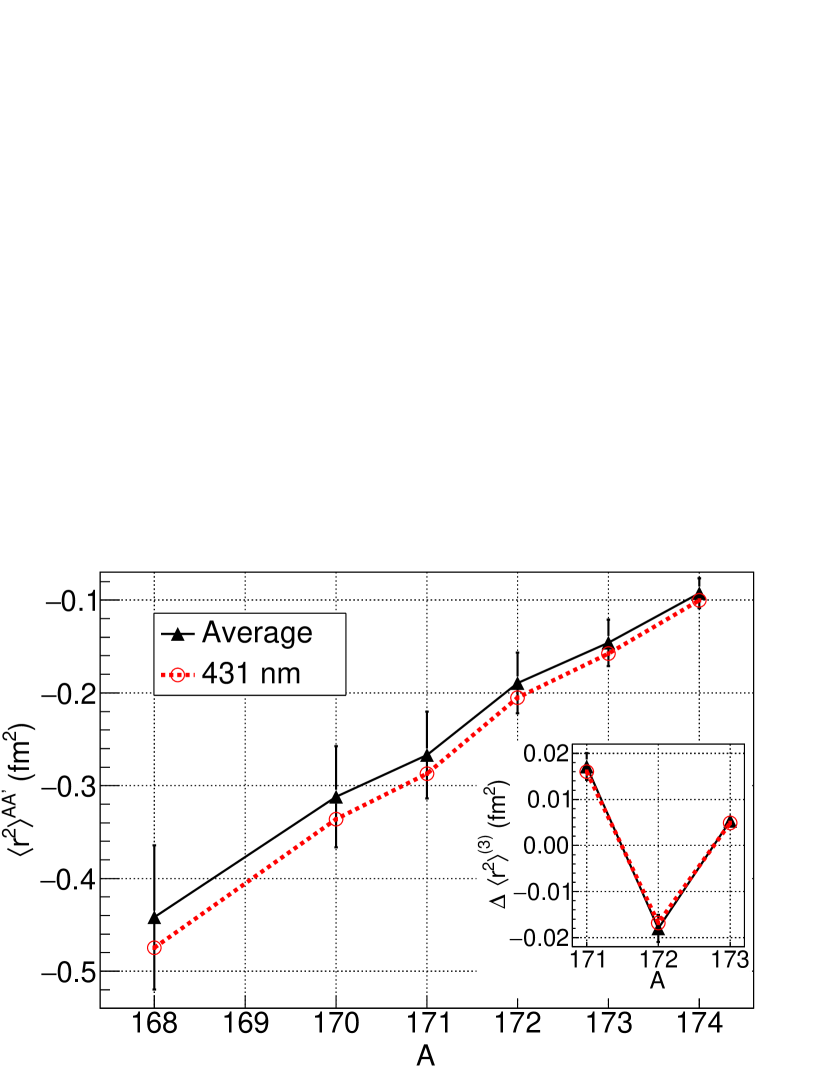
Figure 2: $\langle r^{2}\rangle^{AA^{\prime}}$ calculated from isotope shifts with $A^{\prime}=176$: red circles show the values obtained from the absolute frequencies of the 431 nm transition, and black triangles show the average over the 399, 431, 556, and 578 nm transitions. The inset shows $\Delta\langle r^{2}\rangle^{(3)}$.

From these data, three point odd-even staggering $\Delta\langle r^{2}\rangle^{(3)}$ is calculated as

$$\Delta\langle r^{2}\rangle^{(3)}=\frac{1}{2}(\langle r^{2}\rangle^{A+1}-2\langle r^{2}\rangle^{A}+\langle r^{2}\rangle^{A-1}).$$ (9)

This is plotted in the inset of Fig. 2. Compared to the odd-even staggering observed in other atoms [40, 41, 42, 43], this effect is relatively large for stable isotopes. This could be attributed to the fact that both the number of protons and neutrons are far from the magic numbers (50 and 82).

IV.3 King Plot

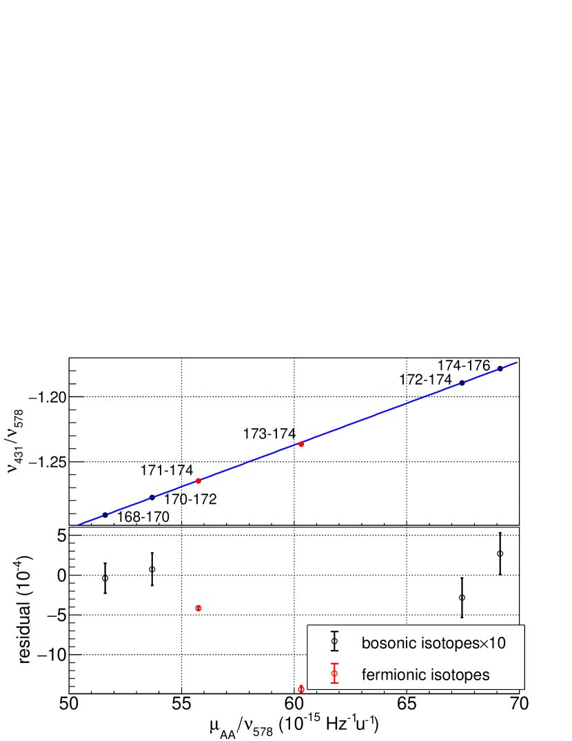
Figure 3: Normalized King plot for the 431 nm transition: the plot is normalized with the 578 nm transition. Texts near each data point show the pair of isotopes that generated the data point. The blue line shows the linear fit of the black data points. See Table 6 in Appendix for the fit parameters. The bottom half displays the residual of each data point from the fitted line. The residuals for the bosonic isotopes (black points) are magnified by a factor of 10.

The normalized King plot between the 431 nm transition and the 578 nm transition following Eq. 3 is shown in Fig. 3. In addition to the data points for bosonic isotopes, data points for fermionic isotopes are plotted. The representative transition frequency for a fermionic isotope is calculated as the center of gravity frequency of the hyperfine levels, and the isotope shift is calculated as the shift from the transition frequency for ¹⁷⁴Yb, so that the data points lie between those of bosonic isotopes and have smaller uncertainties. First, to assess the level of nonlinearity of the King plot, linear fit for the bosonic isotopes is performed by Eq. 3 with only the first two terms on the right hand side. The plot exhibits slight nonlinearity beyond the standard deviation for some data points, as characterized by $\chi^{2}/{\rm ndf}=1.264$. However, as the probability for this level of deviation from $\chi^{2}/{\rm ndf}=1$ is 28.24%, the data points are linear within 95% confidence level.

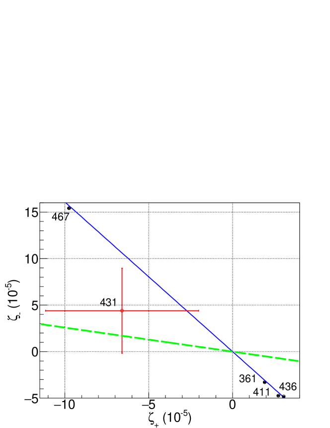
Figure 4: Observed nonlinearity in the normalized King plot displayed on the $(\zeta_{+},\zeta_{-})$ basis. The blue line is the linear fit for the black points with a line on the origin. Best fit is $\zeta_{-}=-1.609(14)\zeta_{+}$, with $\chi^{2}/{\rm ndf}=5.826$. The green dashed line is the nonlinearity pattern generated by the new bosons.

Although the amount of the nonlinearity is consistent with zero, the residual $d^{A}$ for isotope $A$ can be decomposed onto the two dimensional space made by $\zeta_{\pm}=d^{168}-d^{170}\pm(d^{172}-d^{174})$, as introduced in Ref. [7]. The nonlinearity of the 431 nm transition shown in Fig. 4 is consistent with the one-parameter fit for the 361, 411, 436 and 467 nm transitions within one standard deviation. This finding supports the argument made in Ref. [1] that the major part of the nonlinearities in the King plots for Yb originates from several nuclear effects. This consistency observed between the previous results, as well as the almost linear behavior on the King plot, ensures that the measurements are not significantly affected by any systematic shifts beyond the obtained uncertainties.

Table 5: Residual $\delta\nu^{A}$ from the linear fit of the King plot for fermionic isotopes: the residual on the plot is multiplied by $\nu^{AA^{\prime}}_{578}$ and displayed in the unit of kHz.

$\alpha$	$\delta\nu^{171}$ (kHz)	$\delta\nu^{173}$ (kHz)
399	380(218)	3302(266)
431	-754(29)	-792(25)
556	1233(79)	455(76)

$d^{A}$ for the fermionic isotopes is significantly larger than the uncertainties on it, as shown in the bottom half of Fig. 3. To investigate the origin of this offset, the normalized King plots are made for the 399 and 556 nm transitions as well, and $\delta\nu^{A}=d^{A}\nu_{578}^{AA^{\prime}}$ is extracted, as shown in Table 5. On one hand, it is at most $\sim 1$ MHz and thus not significant in older experiments with large uncertainties [44, 45, 46]. On the other hand, with an accuracy of $\sim 10$ kHz, this is significant. $\delta\nu^{171}$, $\delta\nu^{173}$, and $\delta\nu^{173}/\delta\nu^{171}$ are plotted against $Q$ in Table 4, $\Delta_{171,173}/10^{-3}$, $A_{h}^{171}$, $B_{h}^{173}$ , $B_{h}^{173}/A_{h}^{173}$, and $F_{\alpha}$ (See Figs. 8, 9, and 8 in Appendix). Quantities with largest correlation are $B^{173}$ for $\delta\nu_{173}$ and $F_{\alpha}$ for $\delta\nu_{171}$, respectively. $\delta\nu^{173}/\delta\nu^{173}$ does not look to have any good correlation against other quantities. However, it is not evident enough to state these quantities are related, because the $\chi^{2}/{\rm ndf}$ for the linear fit are 7.155 and 5.492, respectively, and both fitted lines do not cross the origin on the two-dimensional plot. One reason why the analysis is inconclusive is because $\delta\nu_{171}$ for the 399 nm transition has a large relative uncertainty. More precise spectroscopy, not only limited to the 399, 431, and 556 nm transitions but also for other narrow-linewidth transitions, is desired to figure out the source of the large $d^{A}$ for fermionic isotopes.

IV.4 Search for new bosons

Together with theoretically calculated $D_{\alpha}$ and the linearity in the King plot for the 431 nm transition, a constraint on the existence of new bosons mediating the force between an electron and a neutron is set. It should be noted that with the relative uncertainty of $\sim 1\times 10^{-5}$ for the isotope shifts in the 431 nm transition, simple analysis with a two-dimensional King plot is good enough, as other sources of uncertainties such as the ones on $\mu^{AA^{\prime}}$ is orders of magnitude smaller. To be most conservative, the effect of the nuclear deformation along the blue line in Fig. 4 is first subtracted from the data point for the 431 nm transition, so that all nonlinearity would arise from the new bosons. As shown in Fig. 4, the effect of the new boson on the $\zeta_{+}-\zeta_{-}$ plane has a slope of -0.2585. On this line, $-6.685\times 10^{5}<v_{ne}D_{431,578}<2.182\times 10^{6}$ is the allowed region for the new bosons with 95% confidence level, which includes $v_{ne}=0$. Thus, such bosons are excluded in the region beyond this, as plotted in Fig. 5. The constraint is more than an order of magnitude worse compared to the most stringent constraint reported in Ref. [1].

With an improvement in the accuracy of the isotope shift measurement for the 431 nm transition, it is expected to increase the sensitivity to the region that has never been investigated before. Fig. 5 shows the sensitivity for the improved accuracy by three orders of magnitude (down to $\sim 18$ Hz), with an assumption that the uncertainty in the isotope shifts for the 431 nm transition is the primary source of the uncertainty. At this point, analysis with three transitions described in Ref. [6] is necessary.

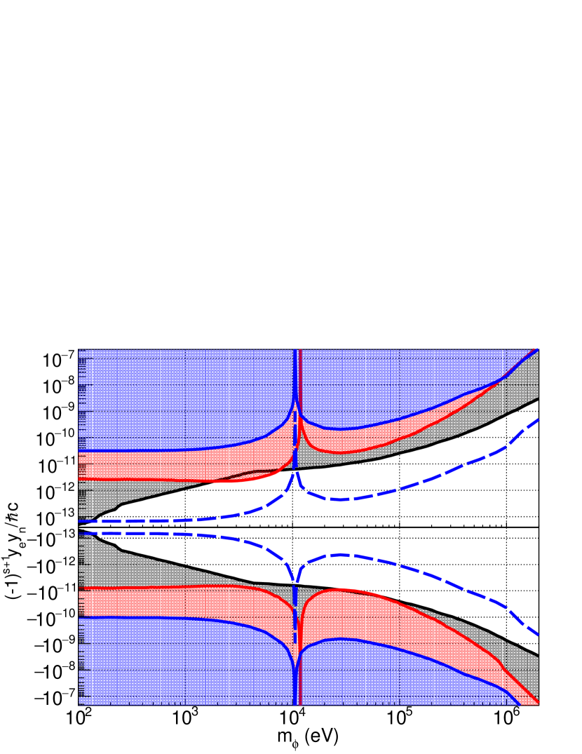
Figure 5: Constraint on the existence of new bosons mediating the force between an electron and a neutron: the black region is excluded by electron $g-2$ measurements and neutron scattering experiments [3]. The red region is the most stringent exclusion reported so far in Ref. [1], obtained from the analysis with the 436, 467, and 578 nm transitions. The blue region is the excluded region by the 431 and 578 nm transitions obtained in this work. The blue dashed line is the expected sensitivity when the accuracy in isotope shifts for the 431 nm is improved by a factor of 1000.

V Conclusion

The full list of absolute frequencies for the 431 nm transition in ^{170,172,173,174,176}Yb is reported, and various analyses based on the data are performed. The King plot analysis did not show as much nonlinearity as reported for other transitions. On one hand, this can ensure the absence of any significant systematic shifts in the measurement, but on the other hand, further improvement in accuracy is desired to investigate the effects inducing the nonlinearity, including the new bosons mediating the force between an electron and a neutron. The hyperfine constants are precisely determined. However, the observed octupole moment is not statistically significant, and this also motivates more precise spectroscopy. The difference in root-mean-square nuclear charge radii between isotopes is determined by averaging isotope shifts of multiple transitions, supporting smaller values compared to some of the previous reports.

Appendix A Summary of the result of theoretical calculation

The result of the theoretical calculation described in Section III is summarized in Table 6. Also, Ref. [6] calculates $K_{578}=-655$ GHz$\cdot$u.

Table 6: Result of the theoretical calculation of the electronic structure in ytterbium: the units of $\nu_{\alpha}$, $F_{\alpha}$, $K_{\alpha}$, $D_{\alpha}$, $K_{\beta,\alpha}$, and $D_{\beta,\alpha}$ are THz, GHz/fm², GHz$\cdot$u, $10^{3}$ THz, GHz$\cdot$u, and $10^{3}$ THz, respectively. $D_{\alpha}$ values are at $m_{\phi}=1$ eV. Ref [1] values are ones calculated by ambit. Experimental values for $\nu_{\alpha}$ are cited from Ref. [23], and the exact value differs by a few GHz according to isotope shifts. Experimental values for $F_{\beta}/F_{\alpha}$ and $K_{\beta\alpha}$ are obtained by the linear fit of King plots for the bosonic isotopes (see Section IV.3).

	this work	Ref. [1]	Ref [22]	Experiment
$\nu_{361}$	875.19	819.47		829.76
$\nu_{399}$	744.82			751.53
$\nu_{411}$	691.88	707.00		729.48
$\nu_{431}$	810.67			695.17
$\nu_{436}$	649.86	679.86		688.35
$\nu_{467}$	727.06	1051.44		642.12
$\nu_{556}$	524.06		543.18	539.39
$\nu_{578}$	500.53	522.78	522.68	518.29
$F_{361}$	-11.988	-13.528
$F_{399}$	-7.020
$F_{411}$	-15.534	-14.715
$F_{431}$	17.771
$F_{436}$	-15.770	-14.968
$F_{467}$	35.260	36.218
$F_{556}$	-9.893		-10.951(21)
$F_{578}$	-9.692	-9.719	-10.848(21)
$K_{361}$	-926
$K_{399}$	412
$K_{411}$	-308	-752
$K_{431}$	10172
$K_{436}$	-158	-661
$K_{467}$	10167	12001
$K_{556}$	-532		-280(72)
$K_{578}$	-527		-288(75)
$D_{361}$		5.6683
$D_{399}$
$D_{411}$	43.37	43.158
$D_{431}$	-94.34
$D_{436}$	49.74	48.634
$D_{467}$	-295.06	-352.38
$D_{556}$
$D_{578}$	-39.49	-42.855
$F_{399}/F_{578}$	0.7243			0.4453(12)
$F_{431}/F_{578}$	-1.8336			-1.62301(8)
$F_{556}/F_{578}$	1.0207			1.00594(26)
$K_{399,578}$	793.7			1332(17)
$K_{431,578}$	9205.7			6430.9(1.4)
$K_{556,578}$	5.929			33.2(4.0)
$D_{431,578}$	-266.7

Appendix B Table for $\langle r^{2}\rangle^{AA^{\prime}}$

Values for $\langle r^{2}\rangle^{AA^{\prime}}$ that were used to generate Fig. 2 are summarized in Table 7.

Table 7: Summary of $\langle r^{2}\rangle^{AA^{\prime}}$. The second column is the valued obtained from the isotope shift of the 431 nm transition. The third column shows the average over the 399, 431, 556, and 578 transition data. The uncertainties for the second column are originated from the spectroscopy only, and the uncertainties in the third column are the standard deviation over the values derived from four transitions.

$A$	$\langle r^{2}\rangle^{AA^{\prime}}$ (fm2)
	431 nm	average
168	-0.474 791 6(21)	-0.442(78)
170	-0.335 961 7(22)	-0.312(54)
171	-0.286 988 3(25)	-0.267(47)
172	-0.205 025 1(23)	-0.189(33)
173	-0.157 682 6(23)	-0.146(25)
174	-0.100 263 6(22)	-0.093(16)
176	0	0

Appendix C Details of the $g$ factor determination

To determine the $g$ factors for the $F=7/2$ and $5/2$ states in ¹⁷³Yb, the bias magnetic field $B_{\parallel}$ along the direction of the propagation of the 431 nm probe beam is varied to obtain the amount of Zeeman splitting. These are shown in Fig. 6. The plot is fitted with the fit function $\Delta\nu=g_{F}\mu_{B}\sqrt{(B_{\parallel}-B_{0})^{2}+B_{\perp}^{2}}$ to accomodate the transverse magnetic field $B_{\perp}$, where $g_{F}$, $B_{0}$, and $B_{\perp}$ are fitting parameters. $g_{F}$ is converted to $g_{J}$ with the relation

$$g_{J}\simeq\frac{2F(F+1)}{F(F+1)-I(I+1)+J(J+1)}g_{F}.$$ (10)

With the uncertainty obtained by the fit, the contribution of the nuclear spin to $g_{F}$ is negligible.

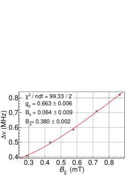
(a) The $F=7/2$ state

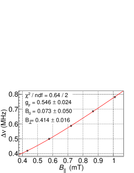
(b) The $F=5/2$ state

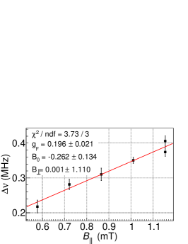
(c) The $F=3/2$ state

Figure 6: The amount of Zeeman splitting $\Delta\nu$ for applied bias magnetic field $B_{\parallel}$ for hyperfine states in ¹⁷³Yb. The uncertainties on the final values for $g_{F}$ in the main text are inflated by $\sqrt{\chi^{2}/{\rm ndf}}$. if $\sqrt{\chi^{2}/{\rm ndf}}>1$.

Appendix D Details of the absolute frequency determination

Several spectra are taken for the absolute frequency measurement for each isotope and hyperfine state to confirm the consistency of the data. Weighted average of these data are regarded as the absolute frequencies, as shown in Fig. 7. The statistical uncertainty is inflated by $\sqrt{\chi^{2}/{\rm ndf}}$ if $\sqrt{\chi^{2}/{\rm ndf}}>1$, and then merged with the systematic uncertainties.

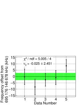
(a) ¹⁷⁶Yb

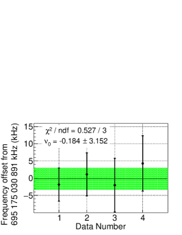
(b) ¹⁷⁴Yb

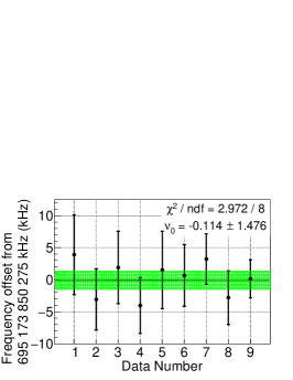
(c) ¹⁷²Yb

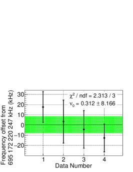
(d) ¹⁷⁰Yb

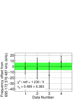
(e) the $F=9/2$ state in ¹⁷³Yb

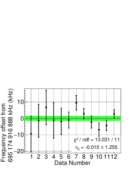
(f) the $F=7/2$ state in ¹⁷³Yb

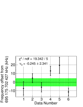
(g) the $F=5/2$ state in ¹⁷³Yb

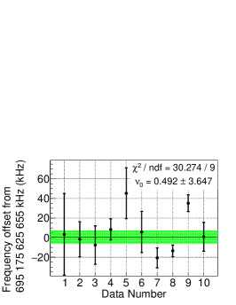
(h) the $F=3/2$ state in ¹⁷³Yb

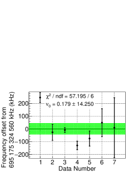
(i) the $F=1/2$ state in ¹⁷³Yb

Figure 7: Plots for determining absolute frequencies: $\nu_{0}$ in the box shows the weighted average. The uncertainty on $\nu_{0}$ is without the inflation by $\sqrt{\chi^{2}/{\rm ndf}}$, whereas the green band is with the inflation if $\sqrt{\chi^{2}/{\rm ndf}}>1$.

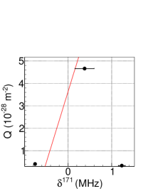
(a)

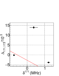
(b)

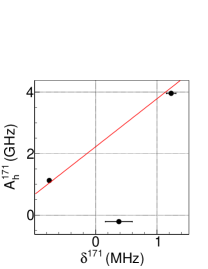
(c)

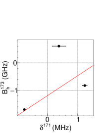
(d)

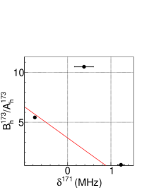
(e)

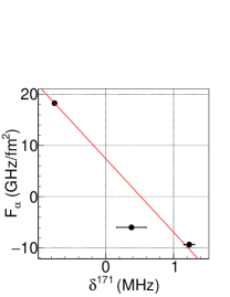
(f)

Figure 8: Plots of the quadrupole moment $Q$ in Table 4, hyperfine anomaly $\Delta_{171,173}/10^{-3}$, hyperfine constants $A_{h}^{171}$, $B_{h}^{173}$, $B_{h}^{173}/A_{h}^{173}$, and field shift $F_{\alpha}$ against $\delta\nu^{171}$: three points correspond to the 399, 431, and 556 nm data. The red line is the linear fit.

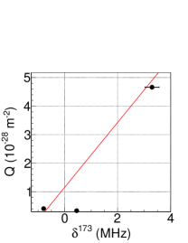
(a)

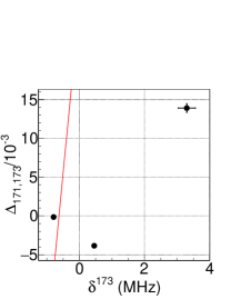
(b)

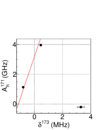
(c)

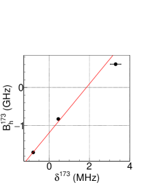
(d)

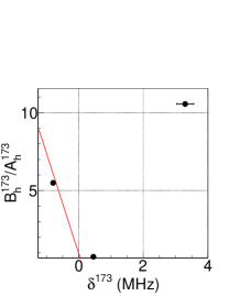
(e)

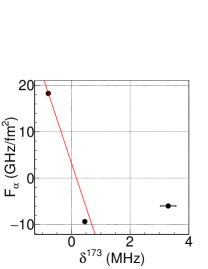
(f)

Figure 9: Plots of the quadrupole moment $Q$ in Table 4, hyperfine anomaly $\Delta_{171,173}/10^{-3}$, hyperfine constants $A_{h}^{171}$, $B_{h}^{173}$, $B_{h}^{173}/A_{h}^{173}$, and field shift $F_{\alpha}$ against $\delta\nu^{171}$: three points correspond to the 399, 431, and 556 nm data. The red line is the linear fit.

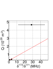
(a)

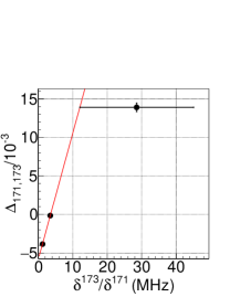
(b)

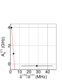
(c)

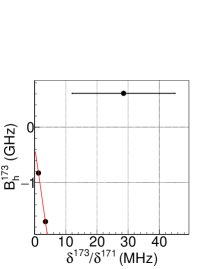
(d)

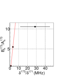
(e)

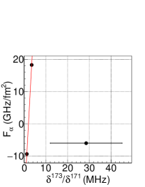
(f)

Figure 10: Plots of the quadrupole moment $Q$ in Table 4, hyperfine anomaly $\Delta_{171,173}/10^{-3}$, hyperfine constants $A_{h}^{171}$, $B_{h}^{173}$, $B_{h}^{173}/A_{h}^{173}$, and field shift $F_{\alpha}$ against $\delta\nu^{173}/\delta\nu^{171}$: three points correspond to the 399, 431, and 556 nm data. The red line is the linear fit.

Appendix E Details of the analysis for the residual from the King plot

Plots of $Q$, $\Delta_{171,173}/10^{-3}$, $A_{h}^{171}$, $B_{h}^{173}$ , $B_{h}^{173}/A_{h}^{173}$, and $F_{\alpha}$ against $\delta\nu^{171}$, $\delta\nu^{173}$, and $\delta\nu^{173}/\delta\nu^{171}$ are shown in Figs. 8, 9, and 10.

Appendix F Formula for hyperfine structure

The absolute frequency for each hyperfine level in ¹⁷³Yb satisfies the following equation.

$$\nu = \nu_{\rm ave}+A_{h}^{173}\frac{K}{2}+B_{h}^{173}\frac{3K(K+1)4I(I+1)J(J+1)}{8I(2I-1)(2J-1)}$$ (11)

$$+C_{h}^{173}\frac{5K^{3}+20K^{2}+4K(I(I+1)+J(J+1)+3-3I(I+1)J(J+1))-20I(I+1)J(J+1)}{4I(I-1)(2I-1)J(J-1)(2J-1)}$$

with $\nu_{\rm ave}$, $A_{h}^{173}$, $B_{h}^{173}$, and $C_{h}^{173}$ being constants that can be determined by measurements, $I$ being nuclear spin, $J$ being total electronic angular momentum, and $K=F(F+1)-I(I+1)-J(J+1)$, with ${\bf F}={\bf I}+{\bf J}$. The 2nd, 3rd, and 4th terms correspond to the magnetic dipole, electric quadrupole, and magnetic octupole components, respectively.

References

- Hur et al. [2022] J. Hur, D. P. L. Aude Craik, I. Counts, E. Knyazev, L. Caldwell, C. Leung, S. Pandey, J. C. Berengut, A. Geddes, W. Nazarewicz, et al., Evidence of two-source King plot nonlinearity in spectroscopic search for new boson, Phys. Rev. Lett. 128, 163201 (2022).
- King [1984] W. H. King, Isotope Shifts in Atomic Spectra, 1st ed., Physics of Atoms and Molecules (Springer New York, NY, 1984).
- Berengut et al. [2018] J. C. Berengut, D. Budker, C. Delaunay, V. V. Flambaum, C. Frugiuele, E. Fuchs, C. Grojean, R. Harnik, R. Ozeri, G. Perez, and Y. Soreq, Probing new long-range interactions by isotope shift spectroscopy, Phys. Rev. Lett. 120, 091801 (2018).
- Mikami et al. [2017] K. Mikami, M. Tanaka, and Y. Yamamoto, Probing new intra-atomic force with isotope shifts, Eur. Phys. J. C 77, 896 (2017).
- Flambaum et al. [2018] V. V. Flambaum, A. J. Geddes, and A. V. Viatkina, Isotope shift, nonlinearity of King plots, and the search for new particles, Phys. Rev. A 97, 032510 (2018).
- Berengut et al. [2020] J. C. Berengut, C. Delaunay, A. Geddes, and Y. Soreq, Generalized King linearity and new physics searches with isotope shifts, Phys. Rev. Res. 2, 043444 (2020).
- Counts et al. [2020] I. Counts, J. Hur, D. P. L. Aude Craik, H. Jeon, C. Leung, J. C. Berengut, A. Geddes, A. Kawasaki, W. Jhe, and V. Vuletić, Evidence for nonlinear isotope shift in Yb+ search for new boson, Phys. Rev. Lett. 125, 123002 (2020).
- Allehabi et al. [2021] S. O. Allehabi, V. A. Dzuba, V. V. Flambaum, and A. V. Afanasjev, Nuclear deformation as a source of the nonlinearity of the king plot in the Yb+ ion, Phys. Rev. A 103, L030801 (2021).
- Tanaka and Yamamoto [2020] M. Tanaka and Y. Yamamoto, Relativistic effects in the search for new intra-atomic force with isotope shifts, Prog. Theor. Exp. Phys. 2020, 103B02 (2020).
- Reinhard et al. [2020] P.-G. Reinhard, W. Nazarewicz, and R. F. Garcia Ruiz, Beyond the charge radius: The information content of the fourth radial moment, Phys. Rev. C 101, 021301 (2020).
- Allehabi et al. [2020] S. O. Allehabi, V. A. Dzuba, V. V. Flambaum, A. V. Afanasjev, and S. E. Agbemava, Using isotope shift for testing nuclear theory: The case of nobelium isotopes, Phys. Rev. C 102, 024326 (2020).
- Müller et al. [2021] R. A. Müller, V. A. Yerokhin, A. N. Artemyev, and A. Surzhykov, Nonlinearities of King’s plot and their dependence on nuclear radii, Phys. Rev. A 104, L020802 (2021).
- Solaro et al. [2020] C. Solaro, S. Meyer, K. Fisher, J. C. Berengut, E. Fuchs, and M. Drewsen, Improved isotope-shift-based bounds on bosons beyond the standard model through measurements of the interval in Ca+, Phys. Rev. Lett. 125, 123003 (2020).
- Rehbehn et al. [2021] N.-H. Rehbehn, M. K. Rosner, H. Bekker, J. C. Berengut, P. O. Schmidt, S. A. King, P. Micke, M. F. Gu, R. Müller, A. Surzhykov, and J. R. C. López-Urrutia, Sensitivity to new physics of isotope-shift studies using the coronal lines of highly charged calcium ions, Phys. Rev. A 103, L040801 (2021).
- Rehbehn et al. [2023] N.-H. Rehbehn, M. K. Rosner, J. C. Berengut, P. O. Schmidt, T. Pfeifer, M. F. Gu, and J. R. C. López-Urrutia, Narrow and ultranarrow transitions in highly charged Xe ions as probes of fifth forces, Phys. Rev. Lett. 131, 161803 (2023).
- Chang et al. [2023] T. T. Chang, B. B. Awazi, J. C. Berengut, E. Fuchs, and S. C. Doret, New limit on isotope-shift-based bounds for beyond standard model light bosons via King’s linearity in Ca+ (2023), arXiv:2311.17337 [physics.atom-ph] .
- Figueroa et al. [2022] N. L. Figueroa, J. C. Berengut, V. A. Dzuba, V. V. Flambaum, D. Budker, and D. Antypas, Precision determination of isotope shifts in ytterbium and implications for new physics, Phys. Rev. Lett. 128, 073001 (2022).
- Ono et al. [2022] K. Ono, Y. Saito, T. Ishiyama, T. Higomoto, T. Takano, Y. Takasu, Y. Yamamoto, M. Tanaka, and Y. Takahashi, Observation of nonlinearity of generalized King plot in the search for new boson, Phys. Rev. X 12, 021033 (2022).
- Kawasaki et al. [2023] A. Kawasaki, T. Kobayashi, A. Nishiyama, T. Tanabe, and M. Yasuda, Observation of the clock transition at 431 nm in , Phys. Rev. A 107, L060801 (2023).
- Ishiyama et al. [2023] T. Ishiyama, K. Ono, T. Takano, A. Sunaga, and Y. Takahashi, Observation of an inner-shell orbital clock transition in neutral ytterbium atoms, Phys. Rev. Lett. 130, 153402 (2023).
- Kahl and Berengut [2019] E. Kahl and J. Berengut, AMBiT: A programme for high-precision relativistic atomic structure calculations, Comput. Phys. Commun. 238, 232 (2019).
- Schelfhout and McFerran [2021] J. S. Schelfhout and J. J. McFerran, Isotope shifts for yb lines from multiconfiguration Dirac-Hartree-Fock calculations, Phys. Rev. A 104, 022806 (2021).
- Kramida et al. [2022] A. Kramida, Yu. Ralchenko, J. Reader, and and NIST ASD Team, NIST Atomic Spectra Database (ver. 5.10), [Online]. Available: https://physics.nist.gov/asd [2023, February 22]. National Institute of Standards and Technology, Gaithersburg, MD. (2022).
- Arimondo et al. [1977] E. Arimondo, M. Inguscio, and P. Violino, Experimental determinations of the hyperfine structure in the alkali atoms, Rev. Mod. Phys. 49, 31 (1977).
- Olschewski [1972] L. Olschewski, Messung der magnetischen kerndipolmomente an freien 43Ca-, 87Sr-, 135Ba-, 137Ba-, 171Yb- und 173Yb-atomen mit optischem pumpen, Z. Phys. 249, 205 (1972).
- Mårtensson-Pendrill et al. [1994] A.-M. Mårtensson-Pendrill, D. S. Gough, and P. Hannaford, Isotope shifts and hyperfine structure in the 369.4-nm 6s-6 resonance line of singly ionized ytterbium, Phys. Rev. A 49, 3351 (1994).
- Stone [2005] N. Stone, Table of nuclear magnetic dipole and electric quadrupole moments, At. Data Nucl. Data Tables 90, 75 (2005).
- Das et al. [2005] D. Das, S. Barthwal, A. Banerjee, and V. Natarajan, Absolute frequency measurements in Yb with uncertainty: Isotope shifts and hyperfine structure in the line, Phys. Rev. A 72, 032506 (2005).
- Wakui et al. [2003] T. Wakui, W.-G. Jin, K. Hasegawa, H. Uematsu, T. Minowa, and H. Katsuragawa, High-resolution diode-laser spectroscopy of the rare-earth elements, J. Phys. Soc. of Jpn 72, 2219 (2003).
- Atkinson et al. [2019] P. E. Atkinson, J. S. Schelfhout, and J. J. McFerran, Hyperfine constants and line separations for the intercombination line in neutral ytterbium with sub-doppler resolution, Phys. Rev. A 100, 042505 (2019).
- Berends and Maleki [1992a] R. W. Berends and L. Maleki, Hyperfine structure and isotope shifts of transitions in neutral and singly ionized ytterbium, J. Opt. Soc. Am. B 9, 332 (1992a).
- Zehnder et al. [1975] A. Zehnder, F. Boehm, W. Dey, R. Engfer, H. Walter, and J. Vuilleumier, Charge parameters, isotope shifts, quadrupole moments, and nuclear excitation in muonic 170–174,176Yb, Nucl. Phys. A 254, 315 (1975).
- Ichihara et al. [1984] T. Ichihara, H. Sakaguchi, M. Nakamura, T. Noro, F. Ohtani, H. Sakamoto, H. Ogawa, M. Yosoi, M. Ieiri, N. Isshiki, and S. Kobayashi, Multipole moments of , , , and from 65 MeV polarized proton inelastic scattering and density dependence of the effective interaction, Phys. Rev. C 29, 1228 (1984).
- Belin and Svanberg [1971] G. Belin and S. Svanberg, Electronic factors, natural lifetimes, and electric quadrupole interaction for Rb87 in the np2P3/2 series of the Rb I spectrum, Phys. Scr. 4, 269 (1971).
- Clark et al. [1979] D. L. Clark, M. E. Cage, D. A. Lewis, and G. W. Greenlees, Optical isotopic shifts and hyperfine splittings for yb, Phys. Rev. A 20, 239 (1979).
- Lee and Boehm [1973] P. L. Lee and F. Boehm, X-ray isotope shifts and variations of nuclear charge radii in isotopes of Nd, Sm, Dy, Yb, and Pb, Phys. Rev. C 8, 819 (1973).
- Sasanuma [1979] T. Sasanuma, Electron Scattering from Deformed Heavy Nuclei, PhD thesis, Massachusetts Institute of Technology (1979).
- Creswell [1977] C. W. Creswell, Electron Scattering Studies of 166Er, 176Yb, and 238U, PhD thesis, Massachusetts Institute of Technology (1977).
- Cooper et al. [1976] T. Cooper, W. Bertozzi, J. Heisemberg, S. Kowalski, W. Turchinetz, C. Williamson, L. Cardman, S. Fivozinsky, J. Lightbody, and S. Penner, Shapes of deformed nuclei as determined by electron scattering: , , , , , and , Phys. Rev. C 13, 1083 (1976).
- An et al. [2022] R. An, X. Jiang, L.-G. Cao, and F.-S. Zhang, Odd-even staggering and shell effects of charge radii for nuclei with even from 36 to 38 and from 52 to 62, Phys. Rev. C 105, 014325 (2022).
- Day Goodacre et al. [2021] T. Day Goodacre, A. V. Afanasjev, A. E. Barzakh, B. A. Marsh, S. Sels, P. Ring, H. Nakada, A. N. Andreyev, P. Van Duppen, N. A. Althubiti, et al., Laser spectroscopy of neutron-rich isotopes: Illuminating the kink and odd-even staggering in charge radii across the shell closure, Phys. Rev. Lett. 126, 032502 (2021).
- Xie et al. [2019] L. Xie, X. Yang, C. Wraith, C. Babcock, J. Bieroń, J. Billowes, M. Bissell, K. Blaum, B. Cheal, L. Filippin, et al., Nuclear charge radii of 62-80Zn and their dependence on cross-shell proton excitations, Phys. Lett. B 797, 134805 (2019).
- de Groote et al. [2020] R. P. de Groote, J. Billowes, C. L. Binnersley, M. L. Bissell, T. E. Cocolios, T. Day Goodacre, G. J. Farooq-Smith, D. V. Fedorov, K. T. Flanagan, S. Franchoo, et al., Measurement and microscopic description of odd–even staggering of charge radii of exotic copper isotopes, Nat. Phys. 16, 620 (2020).
- Berends and Maleki [1992b] R. W. Berends and L. Maleki, Hyperfine structure and isotope shifts of transitions in neutral and singly ionized ytterbium, J. Opt. Soc. Am. B 9, 332 (1992b).
- Loftus et al. [2001] T. Loftus, J. R. Bochinski, and T. W. Mossberg, Optical double-resonance cooled-atom spectroscopy, Phys. Rev. A 63, 023402 (2001).
- van Wijngaarden and Li [1994] W. A. van Wijngaarden and J. Li, Measurement of isotope shifts and hyperfine splittings of ytterbium by means of acousto-optic modulation, J. Opt. Soc. Am. B 11, 2163 (1994).