The Staggered Mesh Method: Accurate Exact Exchange towards the Thermodynamic Limit for Solids

Abstract

In periodic systems, the Hartree-Fock (HF) exchange energy exhibits the slowest convergence of all HF energy components as the system size approaches the thermodynamic limit. We demonstrate that the recently proposed staggered mesh method for Fock exchange energy [Xing, Li, and Lin, Math. Comp., 2024], which is specifically designed to sidestep certain singularities in exchange energy evaluation, can expedite the finite-size convergence rate for the exact exchange energy across a range of insulators and semiconductors when compared to the regular and truncated Coulomb methods. This remains true even for two computationally cheaper versions of this new method, which we call Non-SCF and Split-SCF staggered mesh. Additionally, a sequence of numerical tests on simple solids showcases the staggered mesh method’s ability to improve convergence towards the thermodynamic limit for band gaps, bulk moduli, equilibrium lattice dimensions, energies, and phonon force constants.

1 Introduction

Wavefunction-based methods are becoming increasingly popular for use in electronic structure calculations of solid-state materials.^{1, 2, 3, 4, 5}. However, a longstanding, inherent problem with these methods is the finite-size error; specifically, what finite size of the periodic lattice is required to reach chemical accuracy with respect to the simulation of the infinite lattice, that is, the thermodynamic limit (TDL)? One approach to this problem is to simply increase the number of unit cells along the lattice dimensions; however, doing so will increase the number of electrons, atoms, and basis functions, in the unit cell resulting in greater computational expense. When performing periodic Hartree-Fock (HF) calculations, which is used as a reference for wavefunction methods and used in exact exchange for hybrid Density Functional Theory (DFT), many solid-state quantum chemistry codes use an equivalent yet more efficient approach called k-point sampling, where k is a momentum vector in a Bloch wavefunction. In this approach, the TDL is defined as the limit when the number of k-points sampled over the First Brillouin Zone (FBZ) increases towards infinity.

The standard approach in sampling the FBZ is to use the Monkhorst-Pack (MP) mesh ⁶, which is constructed to evenly sample the FBZ given a number of points to sample along each dimension. Using this mesh, the error in the HF exchange energy as one approaches the TDL decreases as $\mathcal{O}(N_{\mathrm{k}}^{-1/3})$ with an increasing number of k-points $N_{\mathrm{k}}$. This slow convergence rate is primarily due to the excluded divergent term when $|\mathbf{q}+\mathbf{G}|=\mathbf{0}$ in the unscreened Coulomb kernel ⁷. To reduce the error due to the Coulomb singularity, a common practice is to include the Madelung constant correction ^{8, 9}. Interpreting the Madelung constant correction as a singularity subtraction technique allows for a rigorous proof that the finite-size error reduces to $\mathcal{O}(N_{\mathrm{k}}^{-1})$ ⁷.

To reduce the number of k-points sampled and thus the computation time, one can leverage the symmetry of a unit cell for more efficient sampling. For example, sampling all k-points via the MP mesh in a unit cell with high space-group symmetry is redundant; only k-points in the irreducible Brillouin zone (IBZ) need to be sampled, and therefore the computation time can be reduced by a factor approximately equal to the number of symmetry operators in the point group.^{10, 11, 12}. The use of generalized regular k-point grids ^{13, 14, 15}, or even a simple shift of the $\Gamma$-centered MP mesh can be used to accomplish this. However, these methods reduce the calculation runtime by a prefactor that is strongly dependent upon the level of symmetry within the unit cell. Modifications to the Coulomb kernel, including truncation¹⁶ and averaging¹⁷, as well as resolution-of-identity schemes¹⁸ have also been used to either reduce the number of k-points sampled increase computational efficiency when computing exact exchange towards the TDL.

The staggered mesh method is a simple alternative approach for accelerating convergence towards the TDL. Recent studies have demonstrated its effectiveness in improving the asymptotic convergence towards TDL for HF Exchange, Second-order Moller-Plesset Perturbation Theory (MP2), and the Random Phase Approximation (RPA) ^{7, 19, 20}. Consider the two-electron integral in reciprocal space; in the integrand of periodic HF exchange is a denominator that depends on $\left|\mathbf{q}\right|=\left|\mathbf{k}_{j}-\mathbf{k}_{i}\right|$, which is the difference between the $\mathbf{k}$-points of the two Bloch orbitals in a pair density. We exploit the fact that if the two sets of k-points are staggered by a half k-mesh size, then the term with $\mathbf{q}=\mathbf{0}$ is no longer included in the expression for the exchange energy. Under the condition of removable discontinuity, the convergence rate of HF exchange energy to the TDL can be accelerated to $\mathcal{O}(N_{\mathrm{k}}^{-5/3})$ [Corollary 6.7, Ref. 7]. This acceleration has been demonstrated using a model potential.⁷

In this work, we compare the performance of the staggered mesh method, along with two computationally cheaper variants, with the regular method and the Truncated Coulomb method ^{16, 21} in reducing finite size errors for computing HF exchange energies, band gaps, several insulators. We find that all three versions of the staggered mesh method are competitive in computing HF exchange energies and band gaps, with the original staggered mesh method showing a distinct advantage in computing phonon force constants, lattice parameters, and bulk moduli. Furthermore, this method of k-point selection is highly appealing in that it requires minimal modification to most solid-state quantum chemistry packages that are capable of band structure calculations.

2 Theory

One way to approach the TDL in solid-state calculations is to use the supercell model, where one explicitly repeats the unit cell in one or more directions. For this work, however, we use k-point sampling of the FBZ in reciprocal space, which is equivalent to the supercell model. We focus primarily on the convergence of the exchange energy $E_{\mathrm{K}}$ with respect to $N_{\textbf{\text{k}}}$, which contributes most to the finite size error in the HF theory. For notation, AOs are denoted by $\mu,\nu,\lambda,\sigma$, occupied MOs are denoted by $i,j,k,l$, and virtual MOs are denoted by $a,b,c,d$.

We use the Bloch orbital framework:

$$\psi_{\mu_{\mathbf{k}}}(\mathbf{r})=\frac{1}{\sqrt{N_{\textbf{k}}}}\sum_{\mathbf{R}\in\mathbb{L}}\mathrm{e}^{\mathrm{i}\mathbf{k}\cdot\mathbf{R}}\phi_{\mu}(\mathbf{r}-\mathbf{R}),$$

where $\mathbf{R}$ is a vector in the real space Bravais-lattice, $\mathbb{L}$, and $\phi_{\mu}$ is an atomic orbital (AO). Consider a unit cell $\Omega$ with volume $\left|\Omega\right|$ and a corresponding supercell $\Omega^{s}$ of volume $\left|\Omega^{s}\right|=N_{\textbf{k}}\left|\Omega\right|$. Furthermore, define the pair density as

$$\rho_{\mu_{\mathbf{k}_{\mu}}\nu_{\mathbf{k}_{\nu}}}(\mathbf{r})=\phi_{\mu_{\mathbf{k}_{\mu}}}^{*}\left(\mathbf{r}\right)\phi_{\nu_{\mathbf{k}_{\nu}}}\left(\mathbf{r}\right):=\frac{1}{|\Omega|}\sum_{\mathbf{G}\in\mathbb{L}^{*}}\hat{\rho}_{\mu_{\mathbf{k}_{\mu}}\nu_{\mathbf{k}_{\nu}}}(\mathbf{G})e^{\mathrm{i}\mathbf{G}\cdot\mathbf{r}},$$

where $\hat{\rho}_{\mu_{\mathbf{k}_{\mu}}\nu_{\mathbf{k}_{\nu}}}(\mathbf{G})$ is the Fourier transform of the pair density. Then the two-electron integral in the AO basis is defined as

$$\left(\nu_{\mathbf{k}_{\nu}}\lambda_{\mathbf{k}_{\lambda}}\mid\sigma_{\mathbf{k}_{\sigma}}\mu_{\mathbf{k}_{\mu}}\right) =\int_{\Omega^{s}}\mathrm{~{}d}\mathbf{r}_{1}\int_{\Omega^{s}}\mathrm{~{}d}\mathbf{r}_{2}\psi_{\nu_{\mathbf{k}_{\nu}}}^{*}\left(\mathbf{r}_{1}\right)\psi_{\lambda_{\mathbf{k}_{\lambda}}}\left(\mathbf{r}_{1}\right)(\mathbf{G})V_{\text{coul}}\left(\mathbf{r}_{1},\mathbf{r}_{2}\right)\psi_{\sigma_{\mathbf{k}_{\sigma}}}^{*}\left(\mathbf{r}_{2}\right)\psi_{\mu_{\mathbf{k}_{\mu}}}\left(\mathbf{r}_{2}\right)$$

$$=\frac{1}{\left|\Omega^{S}\right|}\sideset{}{{}^{\prime}}{\sum}_{\mathbf{G}\in\mathbb{L}^{*}}\hat{\rho}_{\nu_{\mathbf{k}_{\nu}}\lambda_{\mathbf{k}_{\lambda}}}(\mathbf{G})\hat{V}_{\mathrm{coul}}\left(\mathbf{q}+\mathbf{G}\right)\hat{\rho}_{\sigma_{\mathbf{k}_{\sigma}}\mu_{\mathbf{k}_{\mu}}}\left(\mathbf{G}_{\mathbf{k}_{\lambda},\mathbf{k}_{\mu}}^{\mathbf{k}_{\nu},\mathbf{k}_{\sigma}}-\mathbf{G}\right).$$ (1)

Here, $\mathbf{G}_{\mathbf{k}_{\lambda},\mathbf{k}_{\mu}}^{\mathbf{k}_{\nu},\mathbf{k}_{\sigma}}:=\mathbf{k}_{\lambda}+\mathbf{k}_{\mu}-\mathbf{k}_{\nu}-\mathbf{k}_{\sigma}\in\mathbb{L}^{*}$ by crystal momentum conservation, $\mathbf{q}=\mathbf{k}_{\lambda}-\mathbf{k}_{\nu}$ is the k-point difference, $\sum^{\prime}$ denotes that the term where $\mathbf{q}+\mathbf{G}=\mathbf{0}$ is excluded, and $V_{\text{coul}}(\mathbf{r})$ and $\hat{V}_{\text{coul}}(\mathbf{G})$ are the Coulomb kernel in real and reciprocal space respectively. We use both the default periodic Coulomb kernel in 3D $\hat{V}_{\text{coul}}(\mathbf{G})=\frac{4\pi}{|\mathbf{q}+\mathbf{G}|^{2}}$ and the truncated coulomb kernel ^{16, 21}. If we define $C_{\mu i}^{\mathbf{k}}$ to be the MO-coefficient matrix,

$$\psi_{i_{\mathbf{k}}}(\mathbf{r})=\sum_{\mu\in n_{ao}}C_{\mu i}^{\mathbf{k}}\psi_{\mu_{\mathbf{k}}}(\mathbf{r}),$$

then the density matrix at that same k, $P^{\mathbf{k}}$, is defined as

$$P_{\mu\nu}^{\mathbf{k}}=\sum_{i\in\mathrm{occ}}C_{\mu i}^{\mathbf{k}}\left(C_{\nu i}^{\mathbf{k}}\right)^{*}.$$ (2)

2.1 Fock exchange energy and its Madelung constant correction

With a finite-size mesh $\mathcal{K}$, the Fock exchange energy per unit cell is computed as

$$E_{K}^{N_{\mathbf{k}}}=\dfrac{1}{N_{\mathbf{k}}}\left(-\frac{1}{2}\sum_{i,j}\sum_{\mathbf{k}_{i},\mathbf{k}_{j}\in\mathcal{K}}(i_{\mathbf{k}_{i}},j_{\mathbf{k}_{j}}|j_{\mathbf{k}_{j}},i_{\mathbf{k}_{i}})\right).$$ (3)

In the TDL with $\mathcal{K}$ converging to $\Omega^{*}$ and $N_{\mathbf{k}}\rightarrow\infty$, the energy converges as

$$E_{K}^{\text{TDL}}=\lim_{N_{\mathbf{k}}\rightarrow\infty}E_{K}^{N_{\mathbf{k}}}=\int_{\Omega^{*}}d\mathbf{k}_{i}\int_{\Omega^{*}}d\mathbf{k}_{j}\ \sum_{i,j}F_{K}^{ij}\left(\mathbf{k}_{j},\mathbf{k}_{i}\right),$$ (4)

where the integrand is

$$F_{K}^{ij}(\mathbf{k}_{j},\mathbf{k}_{i})=-\frac{N_{\mathbf{k}}}{2|\Omega^{*}|^{2}}\sum_{i,j}(i_{\mathbf{k}_{i}},j_{\mathbf{k}_{j}}|j_{\mathbf{k}_{j}},i_{\mathbf{k}_{i}}).$$

Note that each of the ERIs above consists of an $N_{\mathbf{k}}^{-1}$ factor and the overall integrand is independent of $N_{\mathbf{k}}$. From a numerical quadrature perspective, the finite-size energy $E_{K}^{N_{\mathbf{k}}}$ approximates the TDL energy $E_{K}^{\text{TDL}}$ by discretizing the integral of $\mathbf{k}_{i}$ and $\mathbf{k}_{j}$ over $\Omega^{*}\times\Omega^{*}$ by a $\mathcal{K}\times\mathcal{K}$ uniform mesh i.e., a trapezoidal rule. By studying the singularity structure of the integrand $F_{X}^{j,i}(\mathbf{k}_{j},\mathbf{k}_{i})$, Ref. 7 provides a tight estimate of this finite-size error as

$$\left|E_{K}^{\text{TDL}}-E_{K}^{N_{\mathbf{k}}}\right|=\mathcal{O}(N_{\mathbf{k}}^{-\frac{1}{3}}).$$

To further reduce this error, a common approach is to introduce the Madelung constant correction ^{8, 9, 22} to the Coulomb kernel involved in the $E_{K}^{N_{\mathbf{k}}}$ calculation as

$$\hat{V}_{\text{coul}}(\mathbf{G})=\begin{cases}\frac{4\pi}{|\mathbf{G}|^{2}}&\mathbf{G}\neq\mathbf{0}\\ -|\Omega|N_{\mathbf{k}}\xi&\mathbf{G}=\mathbf{0}\end{cases},$$ (5)

which leads to a Madelung-corrected exchange energy calculation as

$$E_{K}^{N_{\textbf{k}},\xi}=E_{K}^{N_{\textbf{k}}}+n_{\mathrm{occ}}\xi.$$ (6)

The Madelung constant $\xi$ above is defined as

$$\xi =\left(\frac{|\Omega^{*}|}{N_{\mathbf{k}}}\sum_{\mathbf{q}\in\mathcal{K}_{\mathbf{q}}}-\int_{\Omega^{*}}d\mathbf{q}\right)\left(\frac{1}{(2\pi)^{3}}\sideset{}{{}^{\prime}}{\sum}_{\mathbf{G}\in\mathbb{L}^{*}}\frac{4\pi e^{-|\mathbf{q}+\mathbf{G}|^{2}/\eta}}{|\mathbf{q}+\mathbf{G}|^{2}}\right)+\sideset{}{{}^{\prime}}{\sum}_{\mathbf{R}\in\mathbb{L}_{\mathcal{K}_{\mathbf{q}}}}\frac{\operatorname{erfc}\left(\eta^{1/2}|\mathbf{R}|/2\right)}{|\mathbf{R}|}-\frac{4\pi}{|\Omega|N_{\mathbf{k}}\eta},$$ (7)

where $\mathcal{K}_{\mathbf{q}}$ is a uniform mesh in $\Omega^{*}$ that contains the $\Gamma$-point and has the same size as $\mathcal{K}$, and $\mathbb{L}_{\mathcal{K}_{\mathbf{q}}}$ is the real space lattice associated with all points $\mathbf{q}+\mathbf{G}$ in reciprocal space with $\mathbf{q}\in\mathcal{K}_{\mathbf{q}}$, $\mathbf{G}\in\mathbb{L}^{*}$. Note that $\xi$ is a constant for any arbitrary $\eta>0$. Connecting to the equivalent supercell model, $\mathbb{L}_{\mathcal{K}_{\mathbf{q}}}$ is exactly the Bravais lattice of the supercell and $\mathbf{q}+\mathbf{G}$ defines the associated reciprocal lattice. This method may also be physically interpreted as placing a probe electron at the origin in a uniform charge-compensating background and calculating the potential energy due to interactions with the electron’s periodic images via Ewald summation^{23, 24}.

The Madelung constant correction reduces the finite-size error of the exchange energy to $\mathcal{O}(N_{\mathbf{k}}^{-1})$⁷. The effectiveness of this correction can be rigorously justified from a numerical quadrature perspective. It turns out that $\mathbf{q}$ in (7) can be interpreted as the momentum transfer vector $\mathbf{k}_{i}-\mathbf{k}_{j}$ in the exchange energy calculation (3), which also explains the definition of $\mathcal{K}_{\mathbf{q}}$ in $\xi$. Plugging the definition of $\xi$ into (6), the two terms in the bracket of (7) effectively replace the numerical quadrature of the leading singular term in the integrand $F^{ij}(\mathbf{k}_{i},\mathbf{k}_{j})$ by its exact integral. As a result, the Madelung constant correction improves the integrand smoothness in the finite-size exchange energy calculation (viewed as a numerical quadrature) and thus results in quadrature error reduction. Such a correction is connected to a common numerical quadrature technique for singular integrals called the singularity subtraction method.

2.2 Staggered Mesh Method for Fock exchange

To approximate the TDL exchange energy as an integral in (4), a general finite-size calculation is to discretize the integrals of $\mathbf{k}_{i}$ and $\mathbf{k}_{j}$ separately using two arbitrary uniform meshes $\mathcal{K}_{i}$ and $\mathcal{K}_{j}$, i.e.,

$$E_{K}^{N_{\textbf{k}}}\left(\mathcal{K}_{i},\mathcal{K}_{j}\right) =\dfrac{|\Omega^{*}|^{2}}{N_{\mathbf{k}}^{2}}\sum_{\mathbf{k}_{i}\in\mathcal{K}_{i},\mathbf{k}_{j}\in\mathcal{K}_{j}}\sum_{i,j}F^{ij}_{K}(\mathbf{k}_{i},\mathbf{k}_{j})$$

$$=\frac{1}{N_{\mathbf{k}}}\left(-\frac{1}{2}\sum_{\mathbf{k}_{i}\in\mathcal{K}_{i},\mathbf{k}_{j}\in\mathcal{K}_{j}}\sum_{i,j}\left(j_{\mathbf{k}_{j}}i_{\mathbf{k}_{i}}\mid i_{\mathbf{k}_{i}}j_{\mathbf{k}_{j}}\right)\right).$$ (8)

In this setting, the regular exchange energy calculation $E_{K}^{N_{\mathbf{k}}}$ in (3) requires the two $\mathbf{k}$-meshes to be the same, i.e., $\mathcal{K}_{i}=\mathcal{K}_{j}=\mathcal{K}$. The Madelung constant correction in (6) to the regular exchange energy calculation can also be generalized accordingly ⁷ for the case with two general uniform meshes $\mathcal{K}_{i}$ and $\mathcal{K}_{j}$.

The staggered mesh method for exchange energy calculation is based on the key observation that the ERI $\left(j_{\mathbf{k}_{j}}i_{\mathbf{k}_{i}}\mid i_{\mathbf{k}_{i}}j_{\mathbf{k}_{j}}\right)$ with zero momentum transfer $\mathbf{q}=\mathbf{k}_{i}-\mathbf{k}_{j}=\mathbf{0}$ can lead to significant finite-size error due to the involved Coulomb singularity at $\mathbf{q}+\mathbf{G}=\mathbf{0}$, both with and without the Madelung constant correction. Part of this error in a regular exchange energy calculation can be traced back to the fact that the same $\mathbf{k}$-mesh is used for both $\mathbf{k}_{i}$ and $\mathbf{k}_{j}$. To eliminate this error source, the staggered mesh method applies two different meshes $\mathcal{K}_{i}$ and $\mathcal{K}_{j}$ in (8) so that there is no ERI with zero momentum transfer in the exchange energy calculation. More specifically, we choose $\mathcal{K}_{i}$ to be an arbitrary uniform mesh $\mathcal{K}$ and define $\mathcal{K}_{j}$ as $\mathcal{K}^{1/2}$ by shifting $\mathcal{K}$ by a half-mesh-size in all directions. See Figure 1 for an illustration of such two $\mathbf{k}$-meshes.

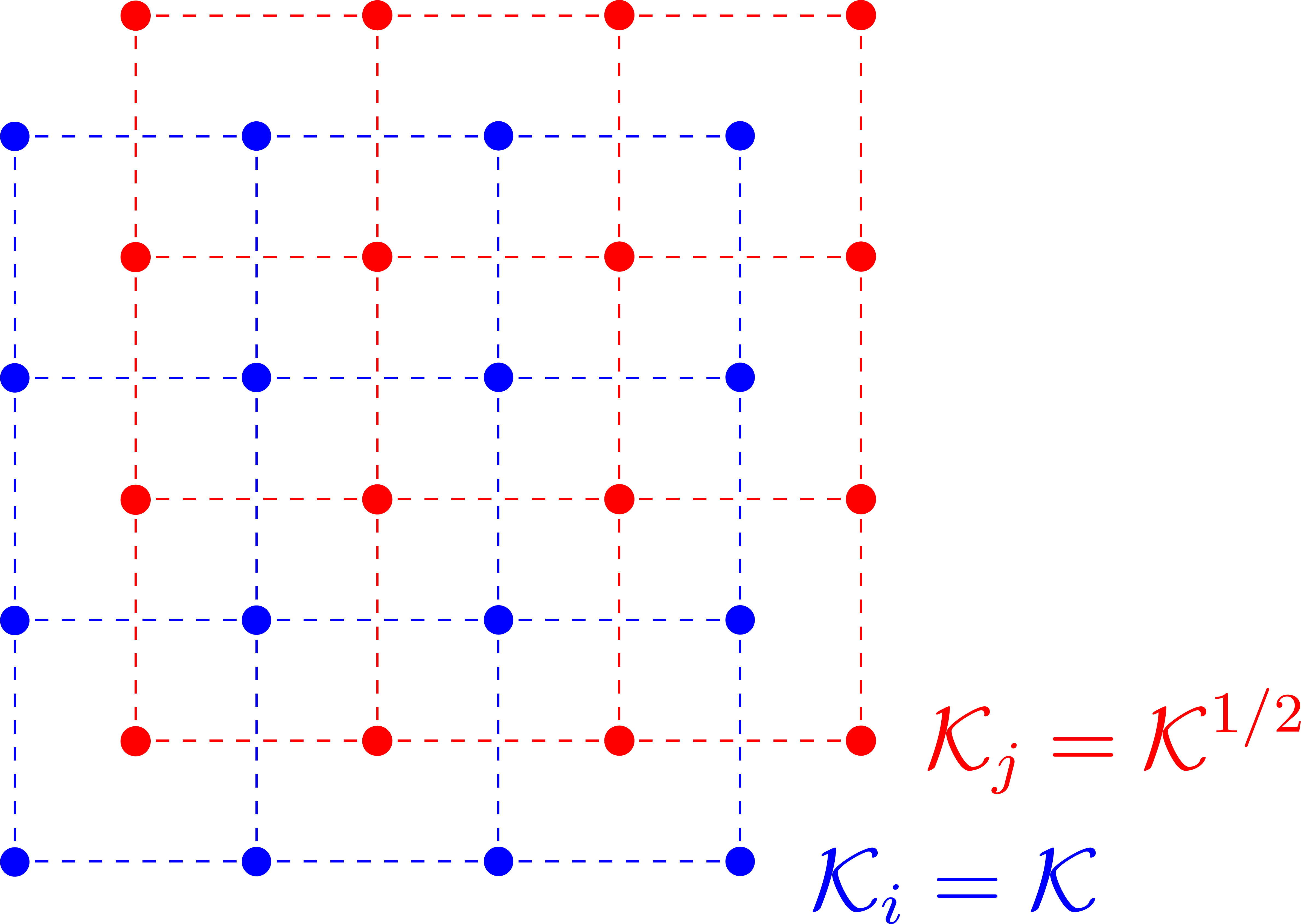
Figure 1: Schematic of the k-point grids used in the staggered mesh method in 2D.

Due to the two staggered $\mathbf{k}$-meshes $\mathbf{k}_{i}\in\mathcal{K}$ and $\mathbf{k}_{j}\in\mathcal{K}^{1/2}$, the minimum images of all possible momentum transfer vectors $\mathbf{q}=\mathbf{k}_{i}-\mathbf{k}_{j}$ in $\Omega^{*}$ no longer lie in $\mathcal{K}_{\mathbf{q}}$ in (7) that contains the $\Gamma$ point. For arbitrary $\mathcal{K}$, those momentum transfer vectors instead form another uniform mesh $\mathcal{K}_{\mathbf{q}}^{1/2}$ which comes from a half-mesh-size shift of $\mathcal{K}_{\mathbf{q}}$ in all directions. From this observation and the numerical quadrature explanation about Madelung constant correction for regular exchange energy calculation, the Madelung-like correction for the staggered mesh method can be generalized accordingly as (Remark 5.2 in Ref. 7)

$$\xi_{1/2} =\lim_{\eta\rightarrow+\infty}\left(\frac{|\Omega^{*}|}{N_{\mathbf{k}}}\sum_{\mathbf{q}\in\mathcal{K}_{\mathbf{q}}^{1/2}}-\int_{\Omega^{*}}d\mathbf{q}\right)\frac{1}{(2\pi)^{3}}\sum_{\mathbf{G}\in\mathbf{L}^{*}}\frac{4\pi e^{-|\mathbf{q}+\mathbf{G}|^{2}/\eta}}{|\mathbf{q}+\mathbf{G}|^{2}}.$$ (9)

This generalization consists of the first two terms in the bracket in (6) with $\mathcal{K}_{\mathbf{q}}$ replaced by $\mathcal{K}_{\mathbf{q}}^{1/2}$ while dropping the remaining two terms in (6) (these two terms decay to zero with $\eta\rightarrow+\infty$). Note that the above term in (9) with any $\eta>0$ can asymptotically reduce the finite-size error and taking $\eta$ to $\infty$ is mainly to be consistent with the standard Madelung constant correction. This correction $\xi_{1/2}$ can be numerically computed by increasing $\eta$, which converges rapidly.

Finally, the staggered mesh method with Madelung-like correction for Fock exchange energy is defined as

$$E_{K}^{N_{\textbf{k}},\xi_{1/2}}\left(\mathcal{K},\mathcal{K}^{1/2}\right)=E_{K}^{N_{\textbf{k}}}\left(\mathcal{K},\mathcal{K}^{1/2}\right)+n_{\mathrm{occ}}\xi_{1/2}.$$ (10)

This approach to calculating the exchange energy not only reduces the errors that arise from the Coulomb singularity term in (1) but also further improves the convergence to $\mathcal{O}(N_{\textbf{k}}^{-5/3})$ under certain conditions ⁷. Specifically, $\mathcal{O}(N_{\textbf{k}}^{-5/3})$ is guaranteed when the unit cell has cubic symmetry. In practice, as will be demonstrated next in the results, to have a cubic unit cell is a sufficient but not necessary condition.

3 Computational Details

3.1 Implementation of Staggered Mesh for HF Exchange

In practical calculations with AOs, the generalized exchange energy in (8) can be formulated and computed as

$$E_{K}^{N_{\textbf{k}}}\left(\mathcal{K}_{i},\mathcal{K}_{j}\right) =-\frac{1}{2N_{\textbf{k}}}\sum_{\mathbf{k}_{i}\in\mathcal{K}_{i},\mathbf{k}_{j}\in\mathcal{K}_{j}}\sum_{\mu,\nu,\lambda,\sigma}P_{\mu\nu}^{\mathbf{k}_{j}}\left(\nu_{\mathbf{k}_{j}}\lambda_{\mathbf{k}_{i}}\mid\sigma_{\mathbf{k}_{i}}\mu_{\mathbf{k}_{j}}\right)P_{\lambda\sigma}^{\mathbf{k}_{i}}$$ (11)

$$=-\frac{1}{2N_{\textbf{k}}}\sum_{\mathbf{k}_{j}\in\mathcal{K}_{j}}\sum_{\mu,\nu}P_{\mu\nu}^{\mathbf{k}_{j}}K_{\nu\mu}^{\mathbf{k}_{j}},$$ (12)

where the exchange matrix is defined as

$$K_{\nu\mu}^{\mathbf{k}_{j}}=\frac{\partial E_{K}}{\partial P_{\mu\nu}^{\mathbf{k}_{j}}}=-\sum_{\mathbf{k}_{i}\in\mathcal{K}_{i}}\sum_{\sigma\lambda}\left(\nu_{\mathbf{k}_{j}}\lambda_{\mathbf{k}_{i}}\mid\sigma_{\mathbf{k}_{i}}\mu_{\mathbf{k}_{j}}\right)P_{\lambda\sigma}^{\mathbf{k}_{i}}.$$ (13)

We introduce the staggered mesh method along with two computationally cheaper versions, which essentially all differ in how they compute the densities $P^{\mathbf{k}}$ in equation (11).

1. (Original) staggered mesh. This delineates the original version of the staggered mesh method. In this procedure, an SCF calculation is done on the combined set of the unshifted and shifted k-points. In other words, this means solving for $P^{\mathbf{k}_{l}}$, where $\mathbf{k}_{l}\in\mathcal{K}^{0+1/2}=\mathcal{K}\cup\mathcal{K}^{1/2}$. If the original unshifted k-mesh has $N_{\textbf{k}}$ k-points, then this SCF calculation solves for a total of $2N_{\textbf{k}}$ k-points. Then, we construct $K^{\mathbf{k}_{j}}$ via (13), where $\mathbf{k}_{j}\in\mathcal{K}_{j}=\mathcal{K}^{1/2}$ and $\mathbf{k}_{i}\in\mathcal{K}_{i}=\mathcal{K}$. Finally, we compute the corrected exchange energy via (12) and (10), As the construction of $K$ dominates the SCF calculation cost with a scaling of $\mathcal{O}(N_{\textbf{k}}^{2})$, this approach is expected to cost approximately 4x as much as a regular HF exchange calculation, making it the most expensive of the three options described here. To keep the subsequent $N_{\textbf{k}}$ convergence plots consistent with the other methods, we say that this version of staggered mesh uses $N_{\mathbf{k}}$ points if the unshifted mesh $\mathcal{K}$ by itself contains $N_{\mathbf{k}}$ points.

2. Split-SCF staggered mesh. In terms of computational expense, an intermediate option is to follow the approach above, except we perform two separate SCF calculations, one on $\mathcal{K}$ and the other on $\mathcal{K}^{1/2}$. This allows us to separately compute $P_{\mu\nu}^{\mathbf{k}_{i}}$ and $P_{\mu\nu}^{\mathbf{k}_{j}}$. This is then followed by the exchange energy computation in (12). Therefore, the cost is expected to be 2x that of an SCF calculation. Here, there will still be some discrepancies arising from the fact that the two densities are effectively being optimized in different mean-field potentials.

3. Non-SCF staggered mesh. This is the cheapest of the three options. First, an SCF calculation is done on $\mathcal{K}$, so $\mathbf{k}_{i},\mathbf{k}_{j}\in\mathcal{K}_{i}=\mathcal{K}$, which gives us $P^{\mathbf{k}_{i}}$. Then, using this density matrix to create an effective potential, we construct $K^{\mathbf{k}_{j}}$ via (13), where $\mathbf{k}_{i}\in\mathcal{K}_{i}=\mathcal{K}$, but $\mathbf{k}_{j}\in\mathcal{K}_{j}=\mathcal{K}^{1/2}$. This exchange matrix is used to build the Fock matrix $F^{\mathbf{k}_{j}}$ which is then diagonalized to yield $P^{\mathbf{k}_{j}}$, that is, the elements of the density matrix on the shifted k-mesh. This is equivalent to performing a band structure calculation on the shifted k-mesh based on the mean-field potential induced by the densities at the unshifted k-mesh. Finally, this new density matrix is used to calculate the staggered mesh exchange energy in (12).

The staggered mesh method, along with the Split and Non-SCF versions, are implemented in a development version of Q-Chem ²⁵. Unless specified otherwise, all geometries were obtained from the Materials Project²⁶, which were optimized using the PBE functional ²⁷. The exceptions are the ammonia crystal, which was obtained from the X23 dataset ²⁸ and the H2 molecule, which is two H atoms at the center of a 6-bohr box with an interatomic distance of 1.4 bohr. All calculations were performed using the SZV-GTH basis set ²⁹ except for the band gap calculations, which were performed with the uncontracted def2-QZVP-GTH basis set³⁰. For computing pair densities in the two-electron integrals, we used the Gaussian and Planewaves (GPW) density fitting scheme, also known as Fast-Fourier-Transform Density Fitting (FFTDF) ^{31, 29}.

4 Results

4.1 Exchange Energies

A total of twelve crystal systems were tested for the convergence of the exact exchange energy $E_{K}$. Among these systems, two are molecular (H2 and ammonia), and the rest are simple solids made of either one (diamond, silicon, graphite) or two elements (LiH; LiF; SiC; hexagonal and cubic BN; AlN; and MgO). Plotting the computed exchange energies versus increasing number of $\mathbf{k}$-points is shown in Fig. 3. For some systems (especially those with large unit cells and hence a large $n_{AO}$), certain lines and data points are missing due to insufficient compute capabilities. In particular, for AlN, the Stagger and Stagger Split-SCF lines stop at $N_{\mathbf{k}}=4^{3}$ and $N_{\mathbf{k}}=5^{3}$ respectively, and for the ammonia crystal, these lines are not available.

The trend that stands out in these results is that all staggered mesh methods display accelerated convergence towards the TDL, even outperforming the Truncated Coulomb method. This is a significant result given that the Truncated Coulomb kernel converges exponentially towards the TDL for insulating systems due to the exponential localization of the single-particle density matrix.^{16, 32} Amongst the three variants of the staggered mesh method, the original version performs the best (albeit by a small margin) for most systems as expected, with the notable exceptions of SiC, Si, Cubic BN, and AlN where the Non-SCF and Split-SCF versions perform slightly better.

However, the original version of the staggered mesh method has a larger memory footprint. For large systems such as the ammonia crystal system and AlN, we can only perform the Non-SCF version of the staggered mesh method.

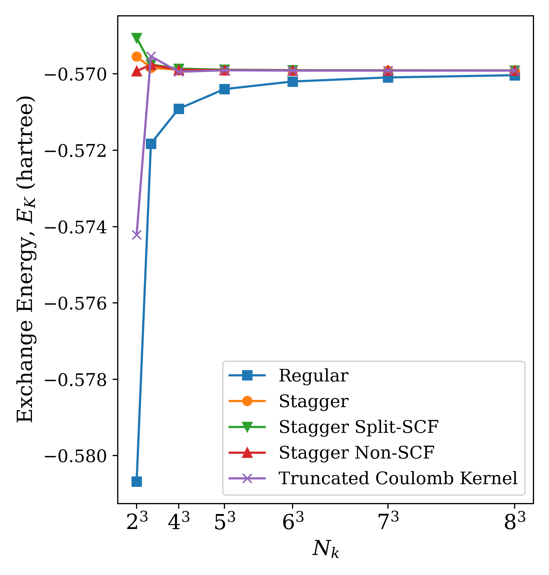
(a) H2

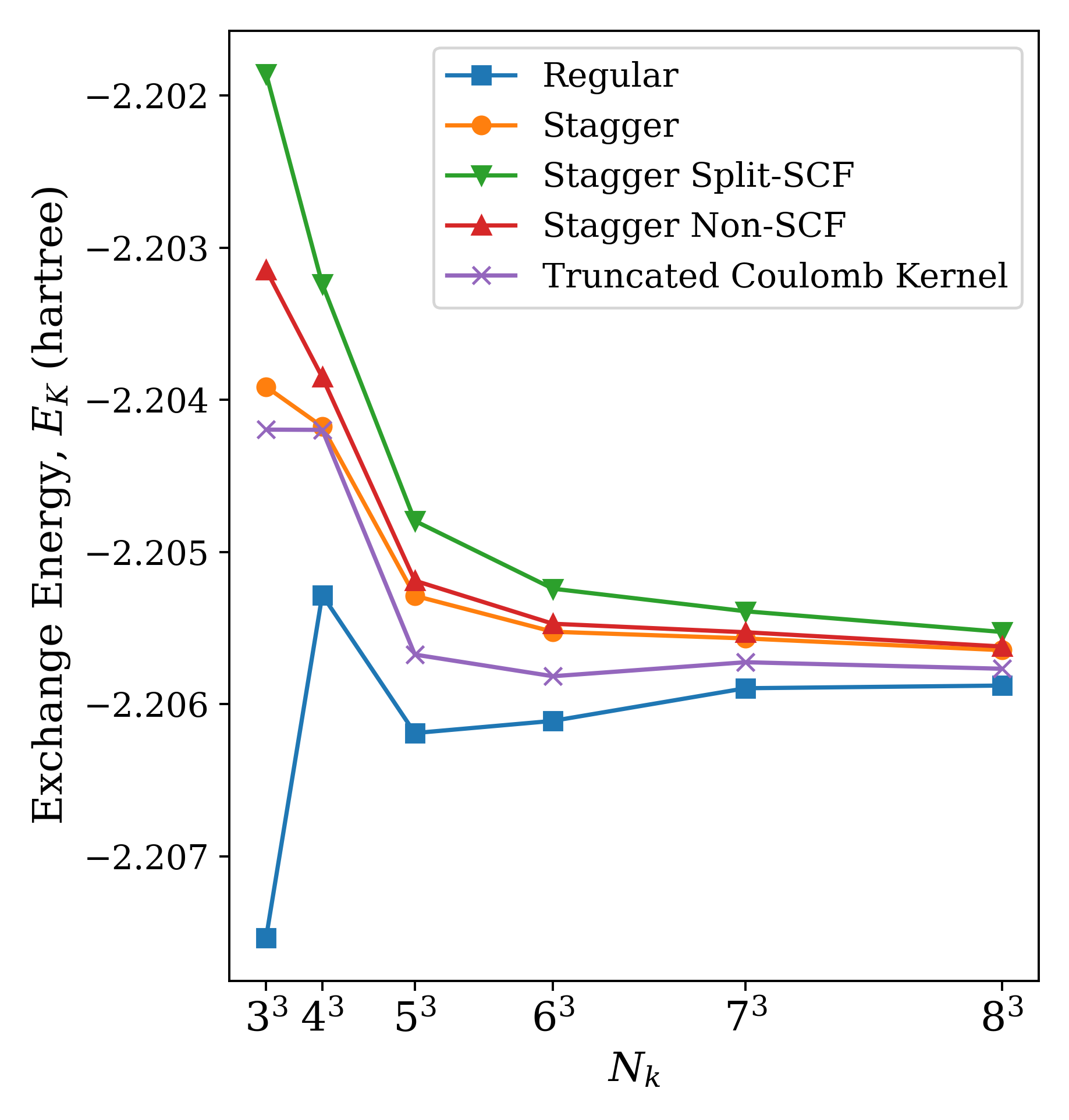
(b) LiH

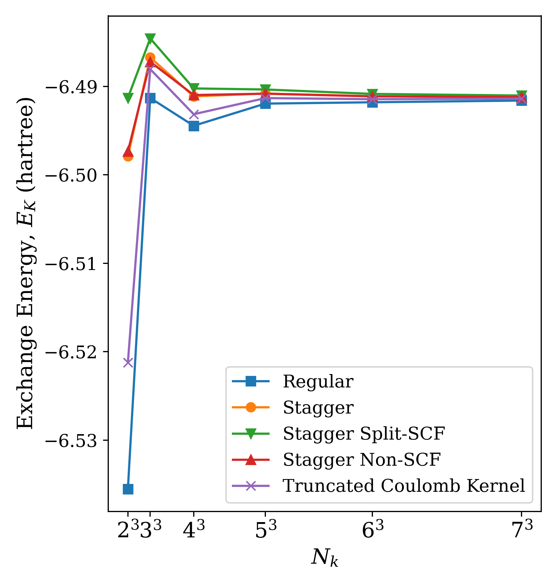
(c) LiF

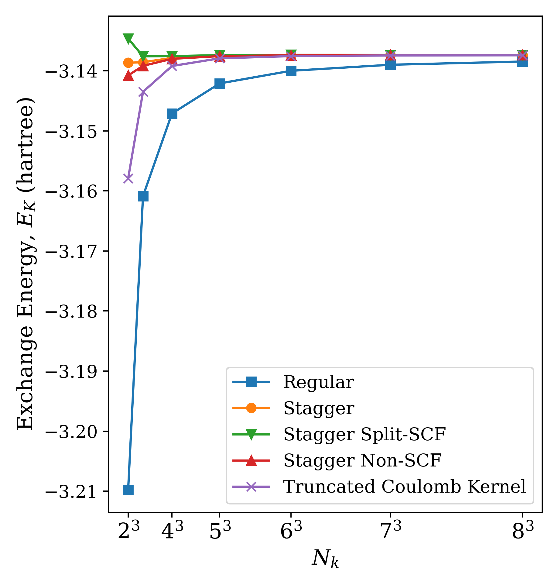
(d) Diamond

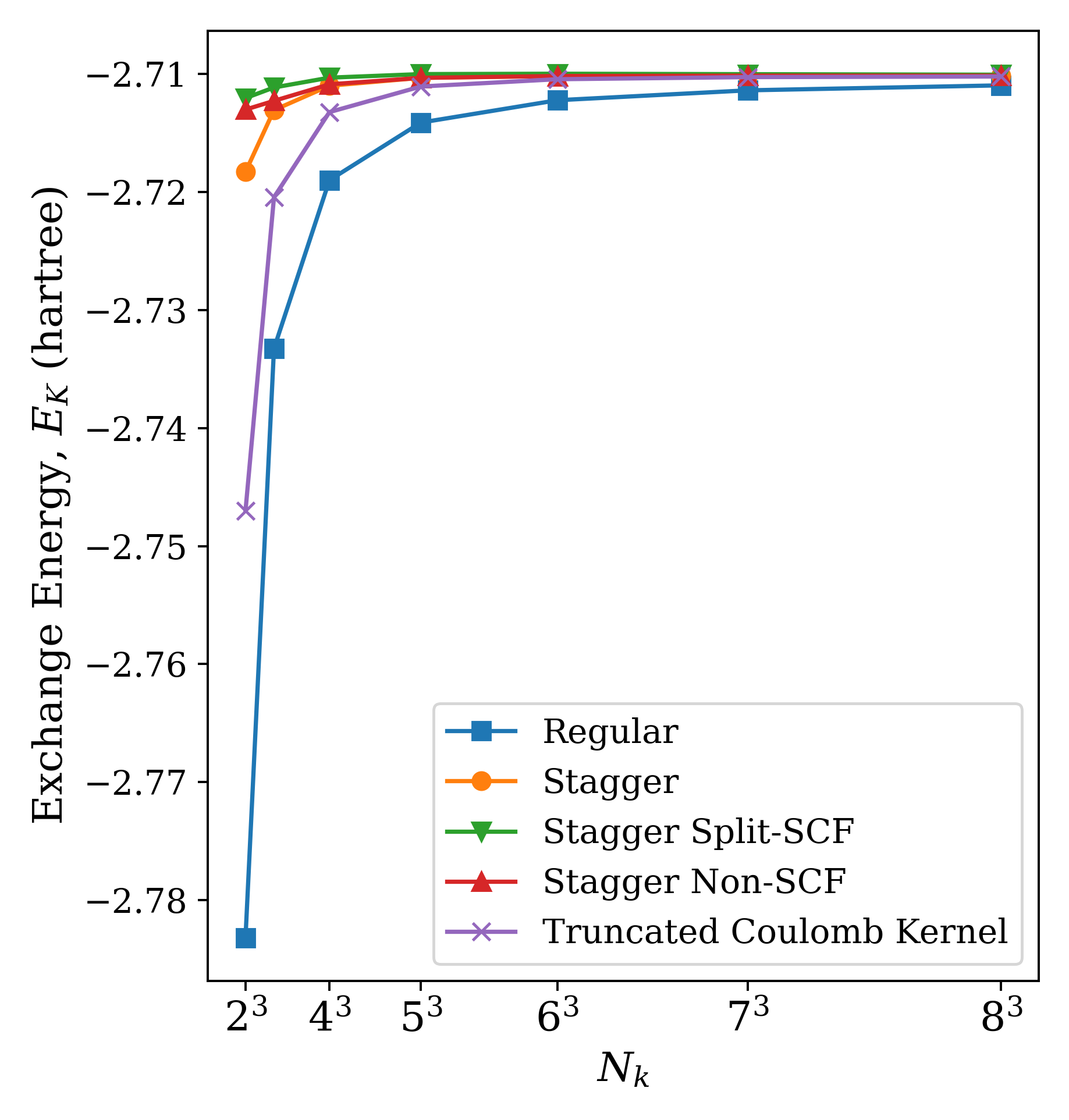
(e) SiC

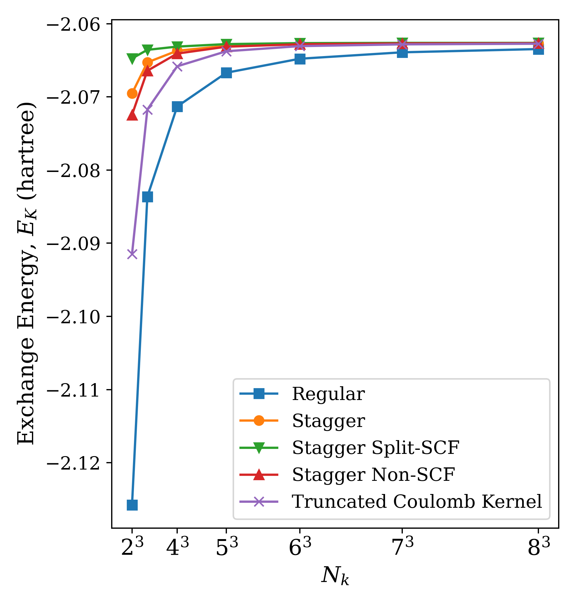
(f) Si

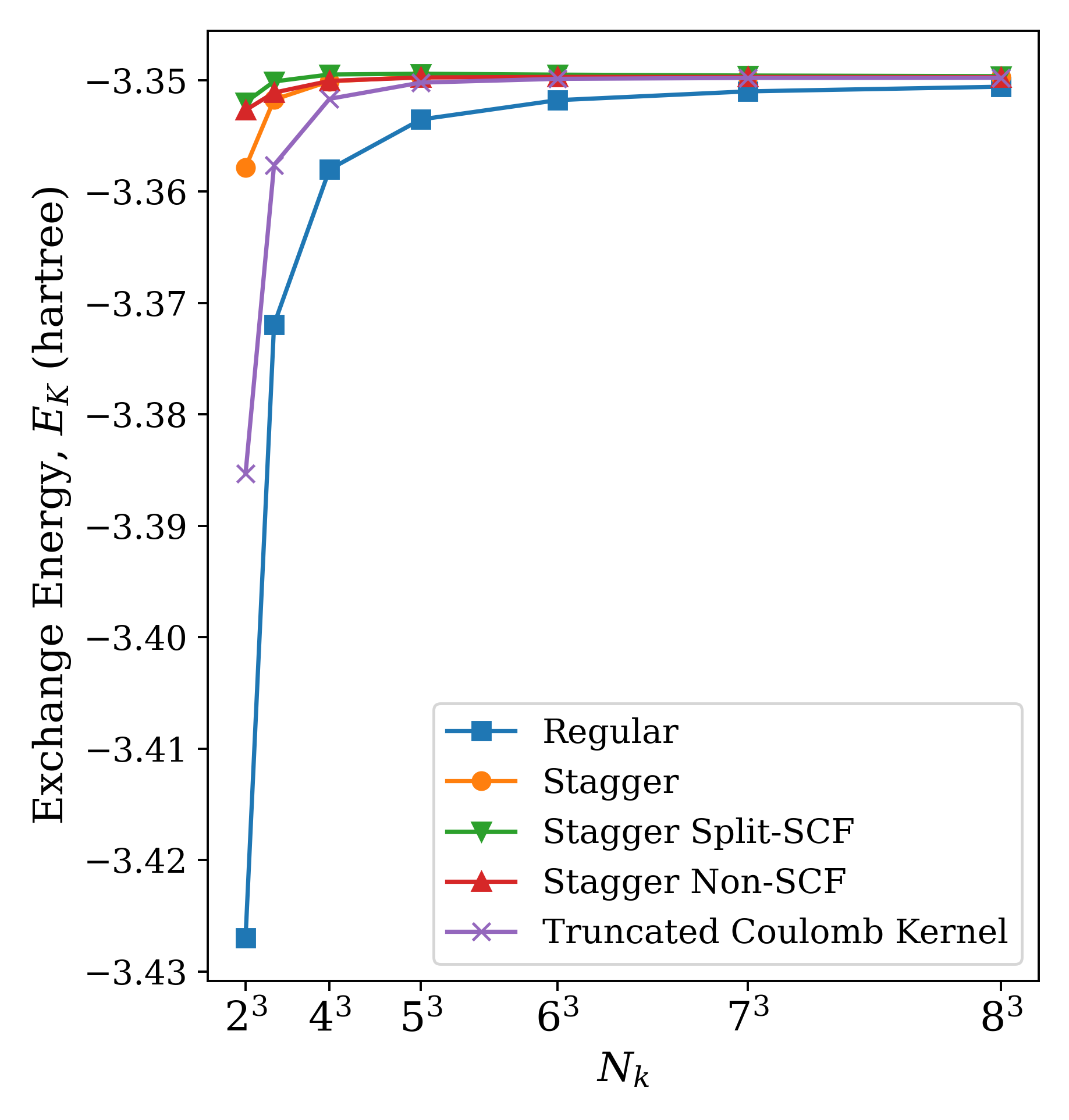
(g) Cubic BN

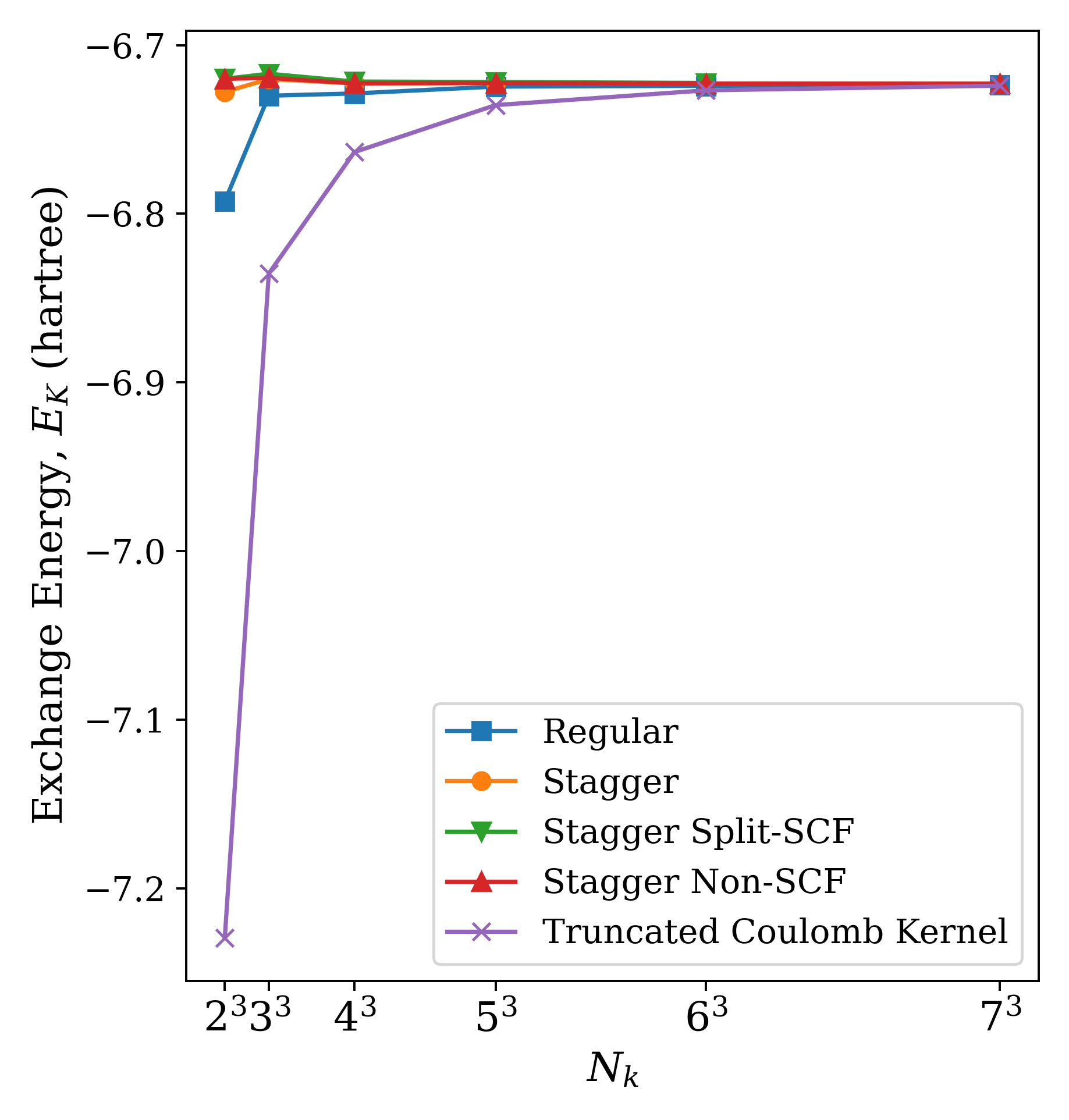
(h) Hexagonal BN

(i) Graphite

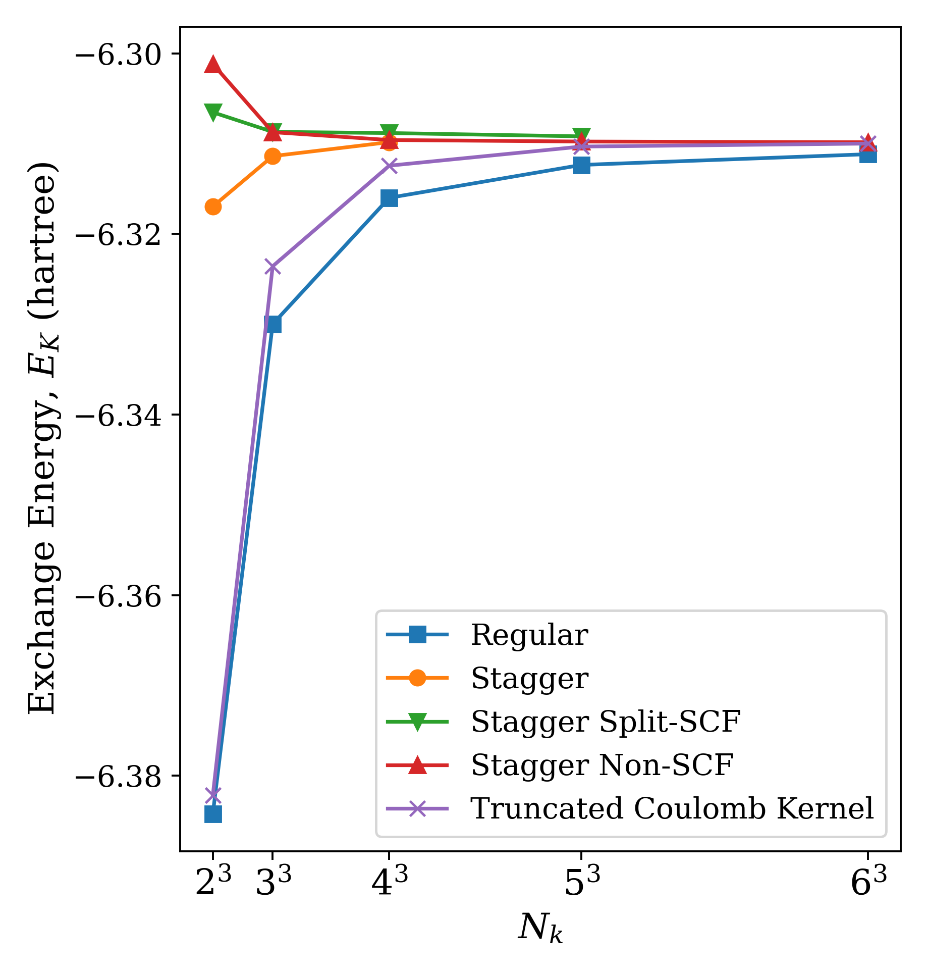
(a) AlN

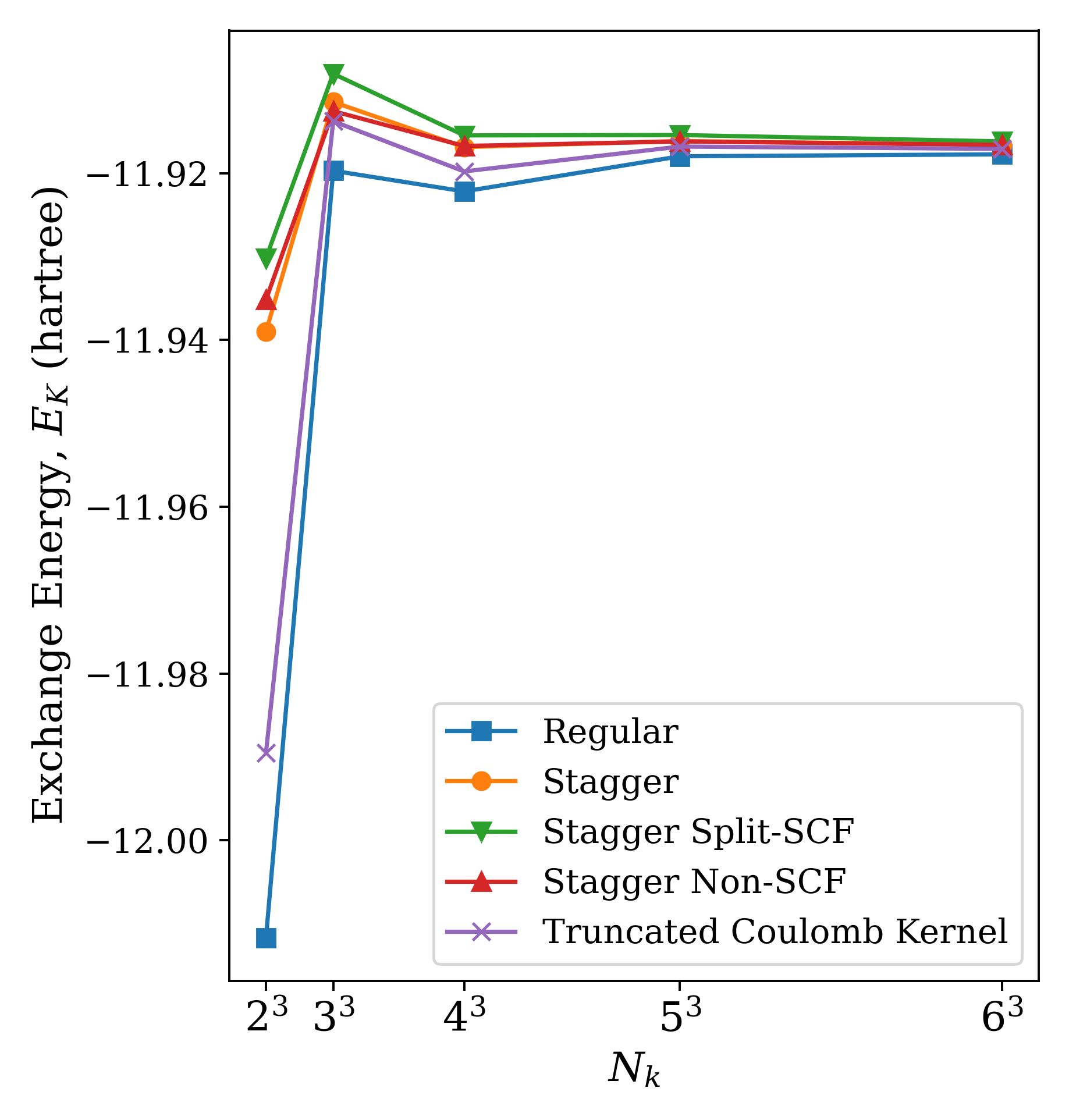
(b) MgO

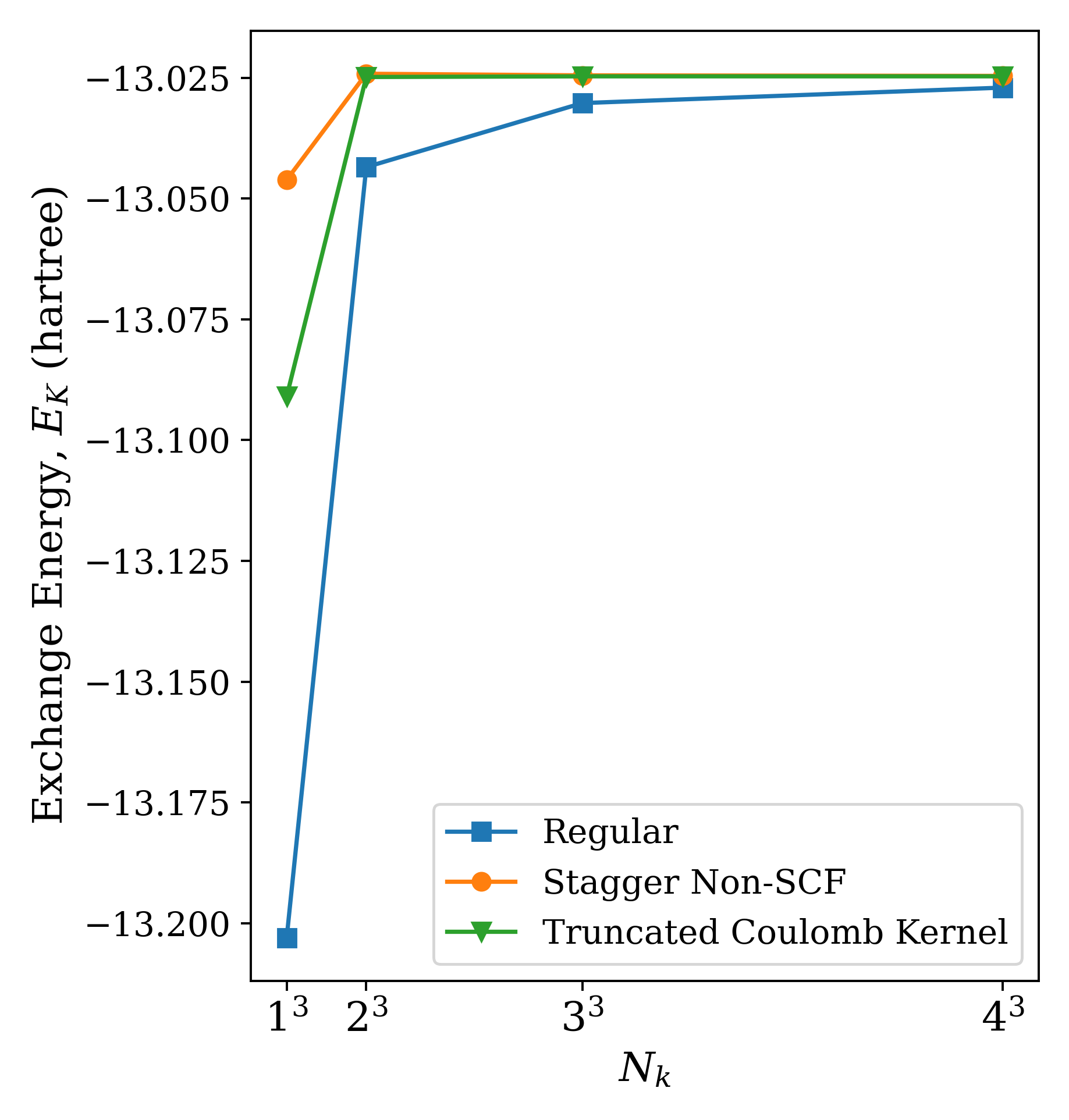
(c) Ammonia Crystal

Figure 3: $N_{\mathbf{k}}$ Convergence Plots

Asymptotic Convergence

In Fig. 4, a power-law curve is fitted to the convergence of energy in diamond and silicon, which both have a rhombohedral primitive cell and exhibit cubic symmetry. In addition to a more favorable prefactor than the regular method, these curves demonstrate a convergence rate faster than $\mathcal{O}(N_{\mathbf{k}}^{-1})$, aligning more closely with the $\mathcal{O}(N_{\mathbf{k}}^{-5/3})$ trend. Conversely, we can expect that the staggered mesh method could become less effective (i.e. converge at the same rate as the regular method) in systems where the unit cell has lower symmetry⁷. To highlight this, we compare diamond (Fig. 2(d)) to graphite (Fig. 2(i)), which both have two carbon atoms in their primitive cells, but graphite has trigonal symmetry instead of cubic. There, we also observe that the staggered mesh method experiences approximately the same degree of oscillation as the regular and Truncated Coulomb methods even when $N_{\mathbf{k}}=6^{3}$ or higher.

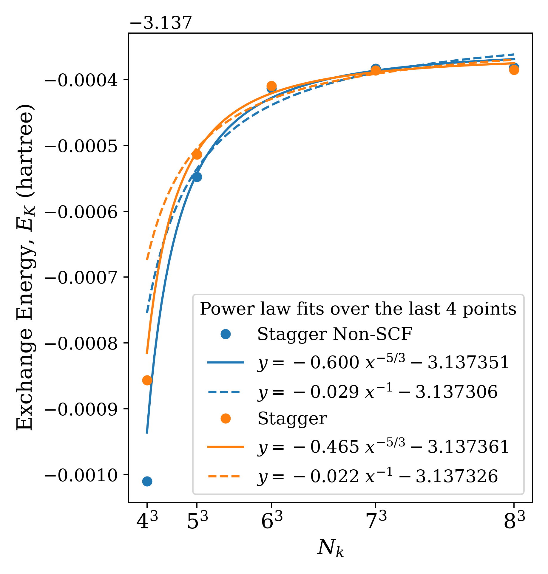
(a) Diamond

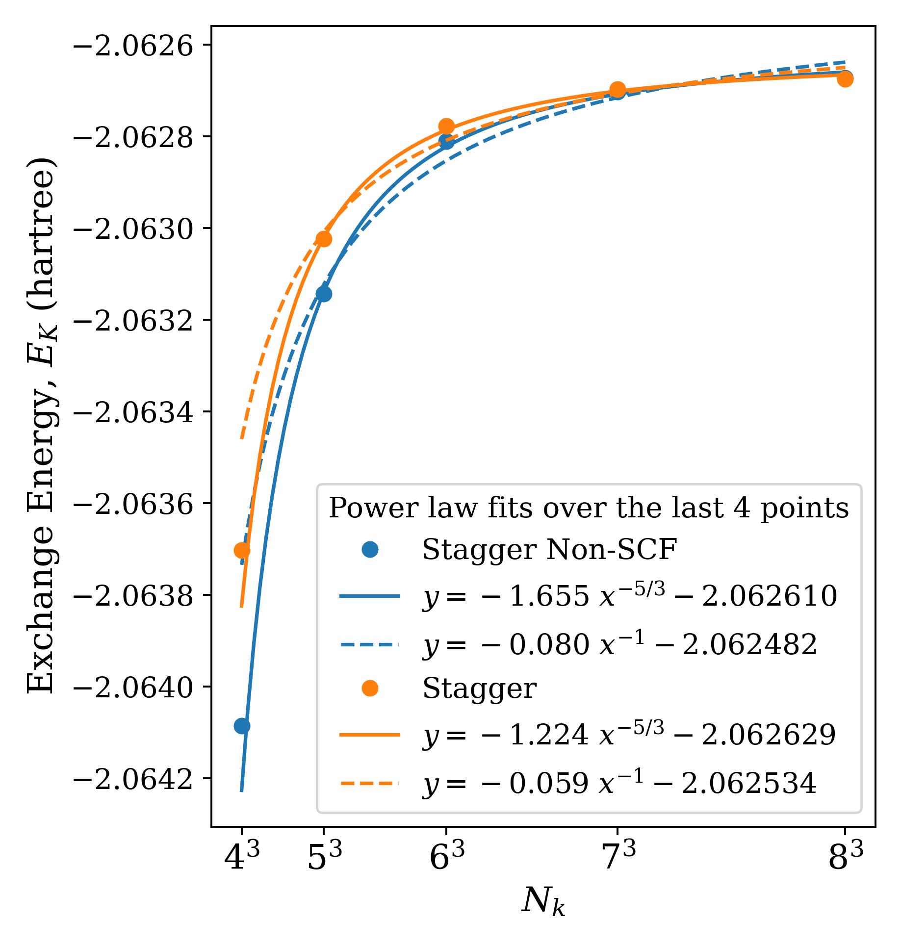
(b) Si

Figure 4: Power Law Fits for the Exchange Energy

Basis Set Effects

We also tested the effect of using the larger GTH-DZVP AO basis set on the performance of the different versions of the staggered mesh method on LiH, BN, silicon, and diamond. The results, shown in Fig. 6 show similar shapes to their SZV-GTH counterparts, with the three staggered mesh methods giving much more similar curves to each other than to the regular method. This points to the use of the Non-SCF version being the most cost-effective variant, while providing similar convergence rates to the original and Split-SCF versions.

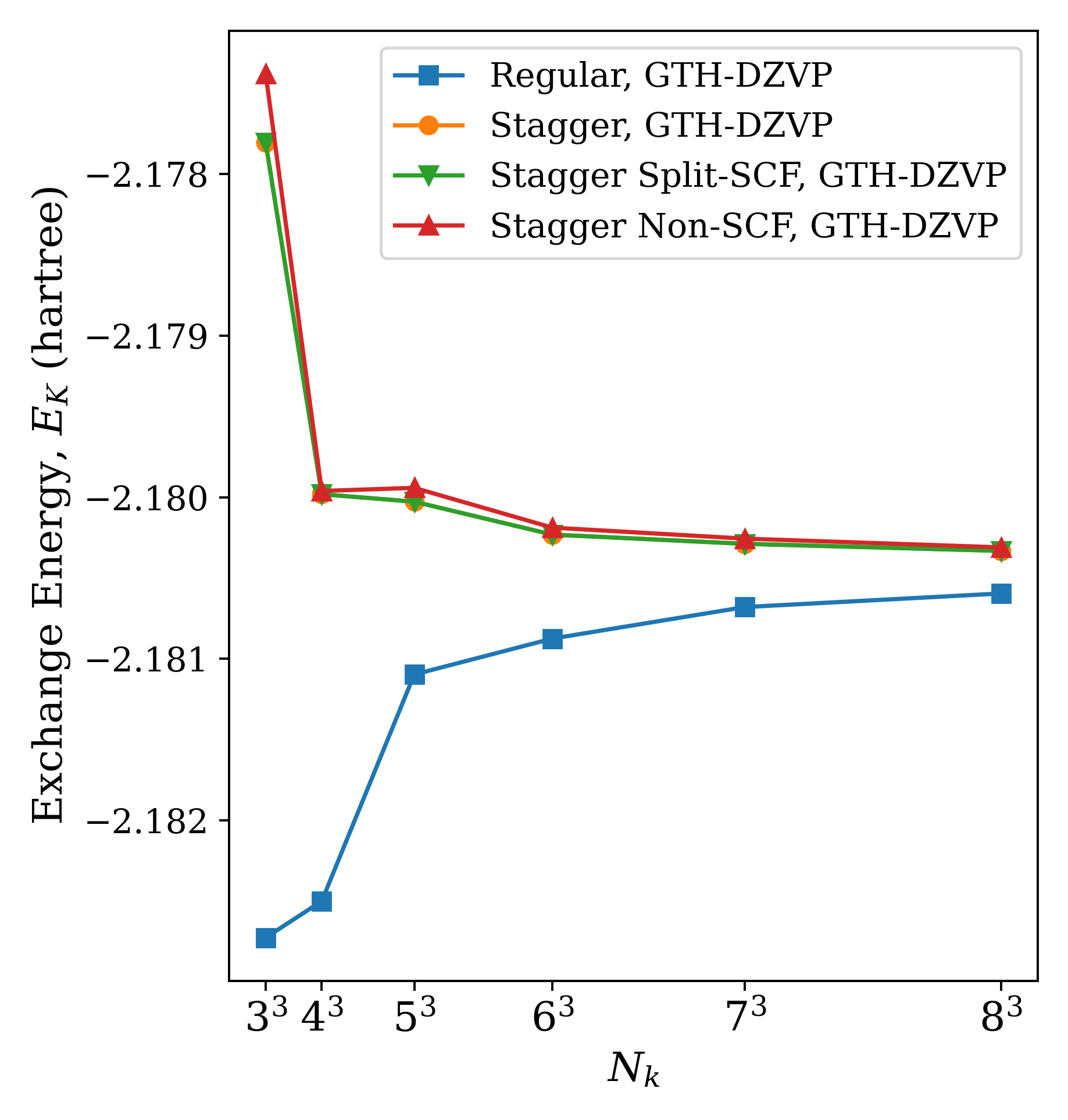
(a) LiH. Compare with Fig. 2(b)

(b) BN. Compare with Fig. 2(g)

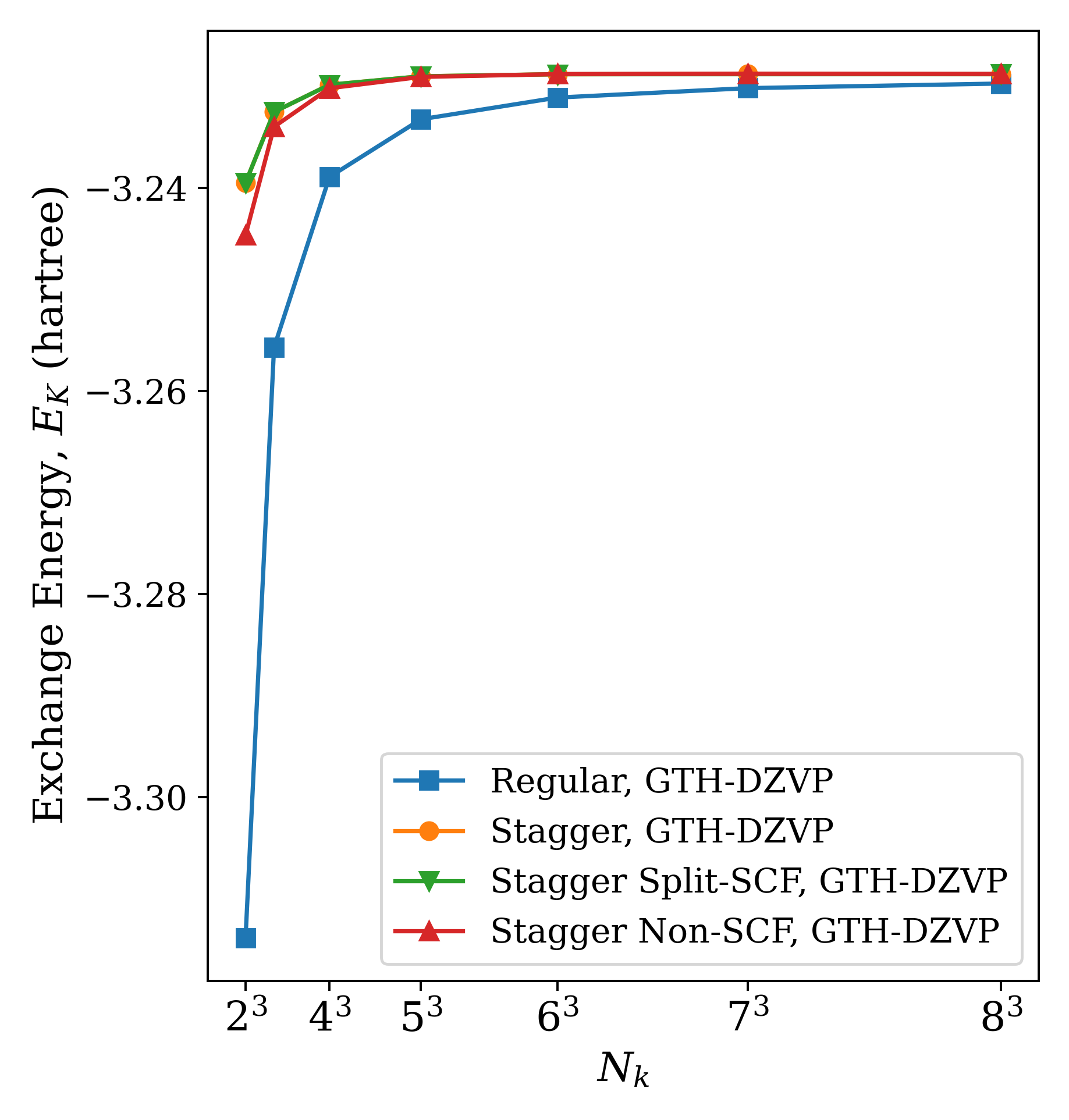
(a) Diamond. Compare with Fig. 2(d)

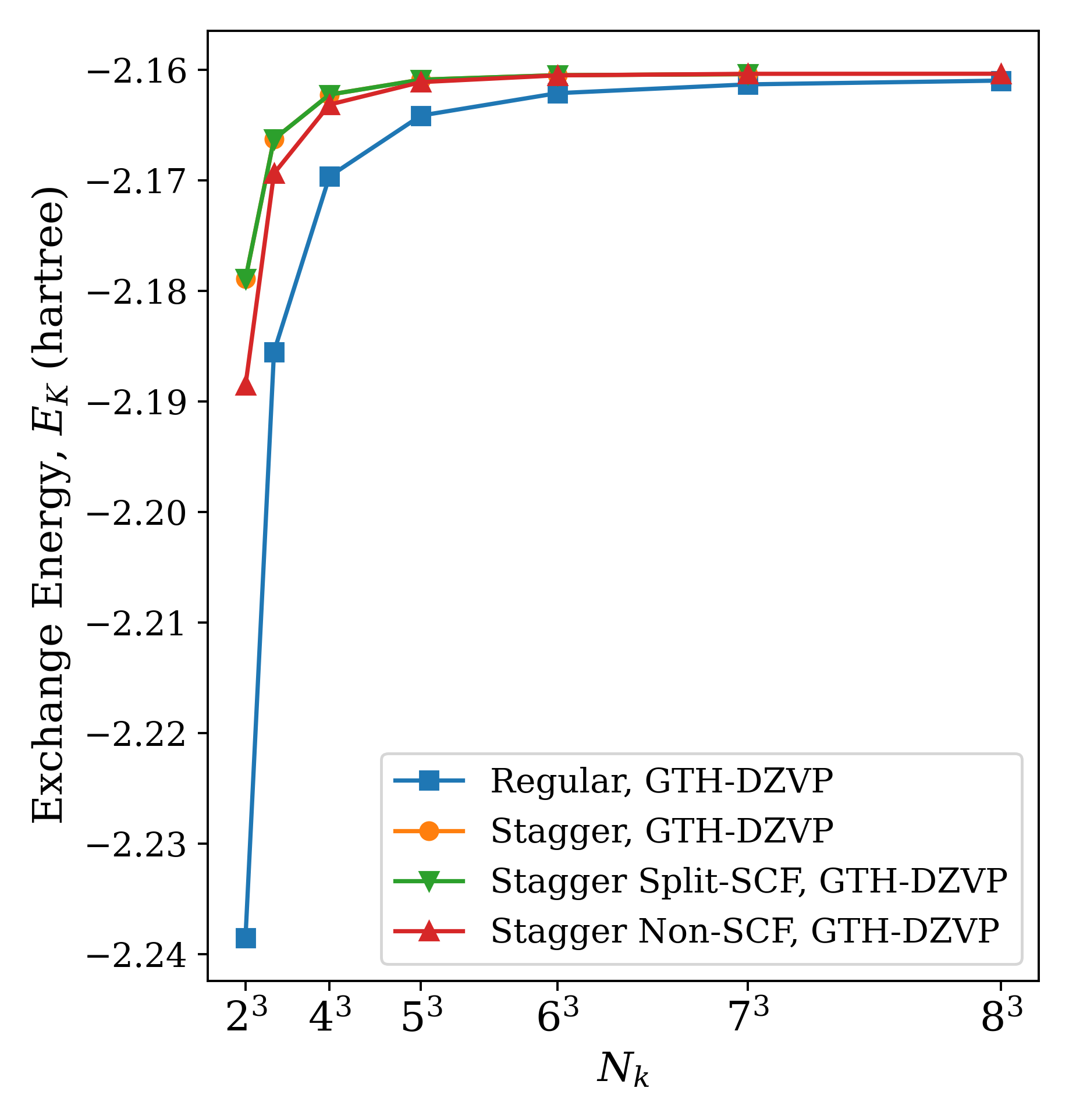
(b) Silicon. Compare with Fig. 2(f)

Figure 6: Finite Size Effects of the Exchange Energy at GTH-DZVP

4.2 Other Physical Observables

Band Gaps

We tested the convergence of band gaps for LiH and diamond towards the TDL. While the former has a direct gap at the $X$ point, the latter has an indirect gap. Similar to the accelerated convergence demonstrated in the calculation of the exchange energy, the staggered mesh method is also expected to converge faster in computing the band gap. This is because the staggered mesh method also computes orbital energies without running into singular terms containing $|\mathbf{q}+\mathbf{G}|=\mathbf{0}$, similar to the proof of the $\mathcal{O}(N_{\textbf{k}}^{-1})$ (or $\mathcal{O}(N_{\textbf{k}}^{-1})$ under the removable discontinuity condition discussed earlier) convergence rates for exchange energy ⁷. We define the exchange contribution to the orbital energy of band $j$ at k-point $\mathbf{k}_{j}\in\mathcal{K}_{j}$ as

$$\varepsilon_{K,j_{\mathbf{k}_{j}}}\left(\mathcal{K}_{i}\right)=-\frac{1}{2N_{k}}\sum_{\mathbf{k}_{i}\in\mathcal{K}_{i}}\sum_{i}\left(j_{\mathbf{k}_{j}}i_{\mathbf{k}_{i}}\mid i_{\mathbf{k}_{i}}j_{\mathbf{k}_{j}}\right)$$ (14)

where $\mathcal{K}_{i}$ is the k-mesh used to converge the SCF calculation. The band gap from the regular method is defined to be when the k-mesh for sampling the band structure is $\mathcal{K}_{j}=\mathcal{K}_{i}$. Then, we define the band gap from the staggered mesh method to be when $\mathcal{K}_{i}=\mathcal{K}^{1/2}_{j}$, that is, the k-mesh used to converge the SCF calculation must be a half shift from the that used to sample the band structure. Therefore, to have a direct comparison between the regular and staggered mesh methods, the $\mathcal{K}_{j}$ must be the same for both. To reduce basis set incompleteness effects, we used the uncontracted def2-QZVP-GTH basis for band gap calculations ³⁰.

For LiH, since the direct band gap is at the $X$ point, which corresponds to the point $\left[0.5,0.5,0\right]$ in the basis of reciprocal lattice vectors, we must set the bands k-mesh $\mathcal{K}_{j}$ as the $\Gamma$-centered MP mesh shifted whose points are all shifted by $\left[0.5,0.5,0\right]$, and therefore, $\mathcal{K}_{i}$ is the $\Gamma$-centered MP mesh shifted whose points are all shifted by $\left[0,0,0.5\right]$. Following the definition of the regular and staggered mesh methods above, we demonstrate the relative rates of convergence of the band gap calculation in Fig. 7(a), with good fits to polynomials of order -1 (regular) and -5/3 (staggered) respectively. The staggered mesh method is clearly superior.

The case for the staggered mesh method becomes somewhat weaker for diamond with its indirect gap. The indirect gap means it becomes more difficult to sample both the HOMO and LUMO in a single MP mesh, which can lead to oscillations as $N_{\mathbf{k}}$ increases as shown in Fig. 7(b). Here, we use the $\Gamma$-centered MP mesh to sample the band structure. Nevertheless, absolute errors are still lower for the staggered mesh method at nearly all $N_{\mathbf{k}}$.

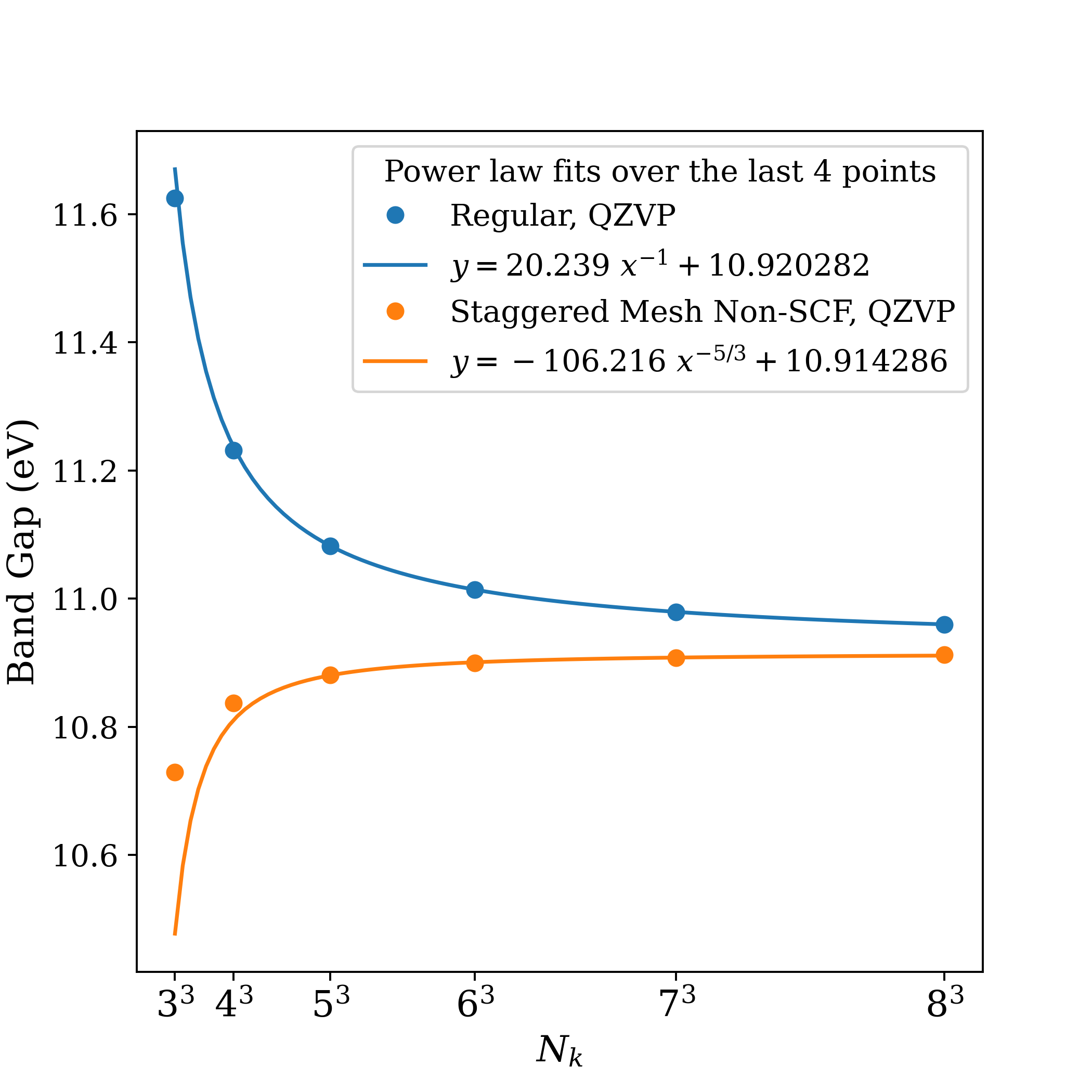
(a) LiH

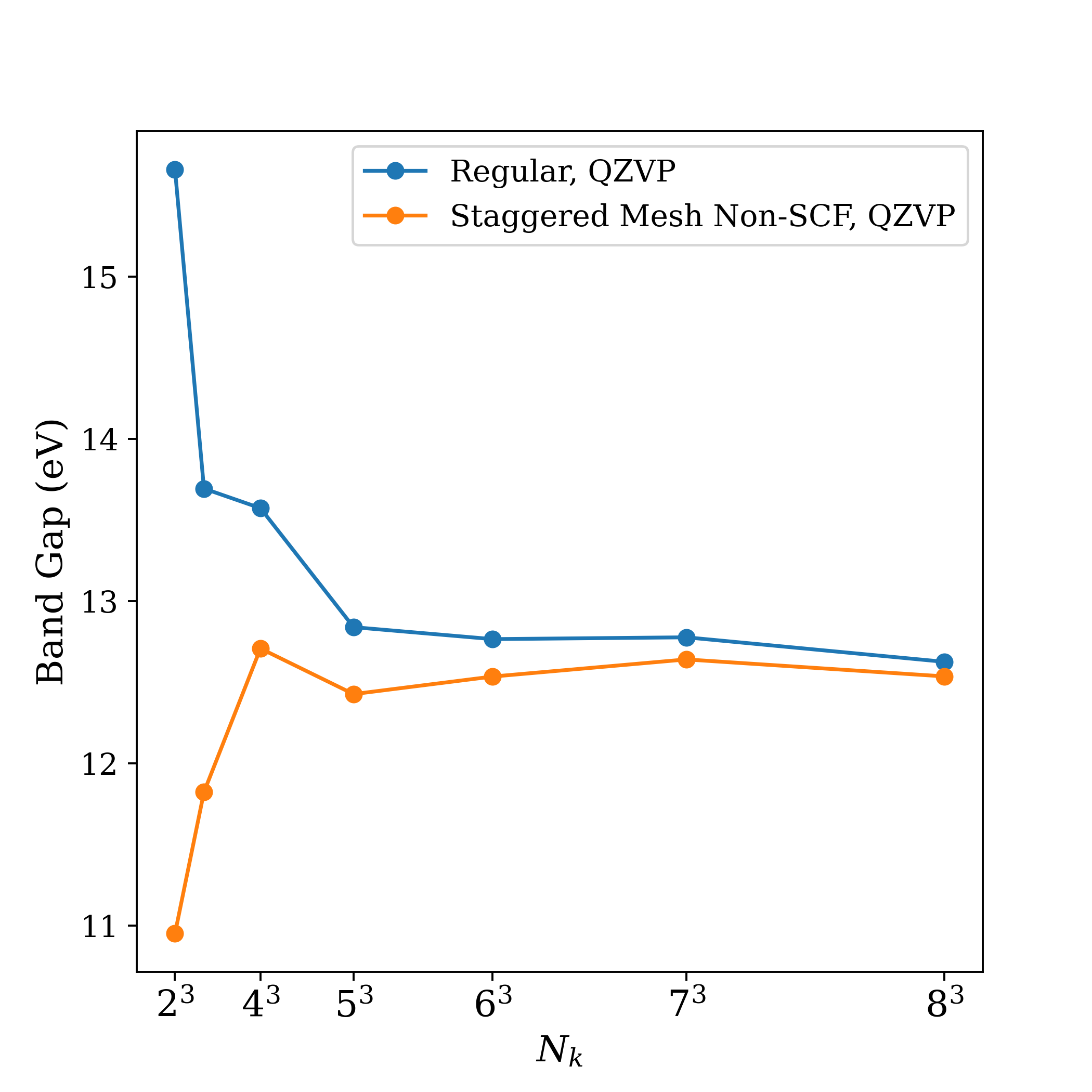
(b) Diamond

Figure 7: Band Gaps

Lattice Parameters and Bulk Moduli

We next demonstrate the effectiveness of the staggered mesh method in computing properties derived from varying the lattice parameter, $a$, of the unit cell. In particular, computing the total energy as a function of $a$ around the equilibrium lattice parameter $a_{0}$ and fitting a Birch-Murnaghan equation of state (EOS) ^{33, 34} allows one to estimate $a_{0}$, the equilibrium total energy $E_{0}$, the bulk modulus $B_{0}$, and the bulk modulus derivative $B^{\prime}_{0}=(\partial B/\partial P)_{T}$ as parameters. The EOS is shown below.

$$E_{\mathrm{total}}(a)=E_{0}+\frac{9V_{0}B_{0}}{16}\left\{\left[\left(\frac{a_{0}}{a}\right)^{2}-1\right]^{3}B_{0}^{\prime}\right.\left.+\left[\left(\frac{a_{0}}{a}\right)^{2}-1\right]^{2}\left[6-4\left(\frac{a_{0}}{a}\right)^{2}\right]\right\}$$ (15)

In Fig. 8 we show the Birch-Murnaghan curves for LiH and Si using each method with $N_{\mathbf{k}}=6^{3}$. The EOS as a function of $N_{\mathbf{k}}$ leads to the data shown in Figs. 9, 11 and 10; the convergence plots of $a_{0}$, $E_{0}$, and $B_{0}$ respectively. These plots paint a stronger picture of the difference in accuracy among the staggered mesh methods. In all plots, the original staggered mesh method performs significantly better than the Split-SCF and Non-SCF variants. Even when considering that the original variant requires double the k-points as Non-SCF, a simple comparison of the original staggered mesh at $N_{\mathbf{k}}=4^{3}=64$ versus the Split- and Non-SCF variants at $N_{\mathbf{k}}=5^{3}=125$ (or the former at $N_{\mathbf{k}}=5^{3}$ vs. the latter at $N_{\mathbf{k}}=6^{3}=216$) shows that the original staggered mesh is still more accurate. In fact, in the convergence of $B_{0}$ in Fig. 9, the Split- and Non-SCF versions appear to do even worse than the regular method at low $N_{\mathbf{k}}$.

Thus, although the Split-SCF and Non-SCF versions of staggered mesh may be more efficient in computing exchange energies, recovering measures of curvature like $B_{0}$ is best done through the original version of staggered mesh. We expect that the superior performance of the original version is due to (1) the invoking of a single SCF calculation on the combined mesh, which means the density matrices used in computing the exchange energy are fully self-consistent with each other, and (2) the other components of total energy such as the two-electron Coulomb matrix $J$ are also being recovered with the higher density k-mesh.

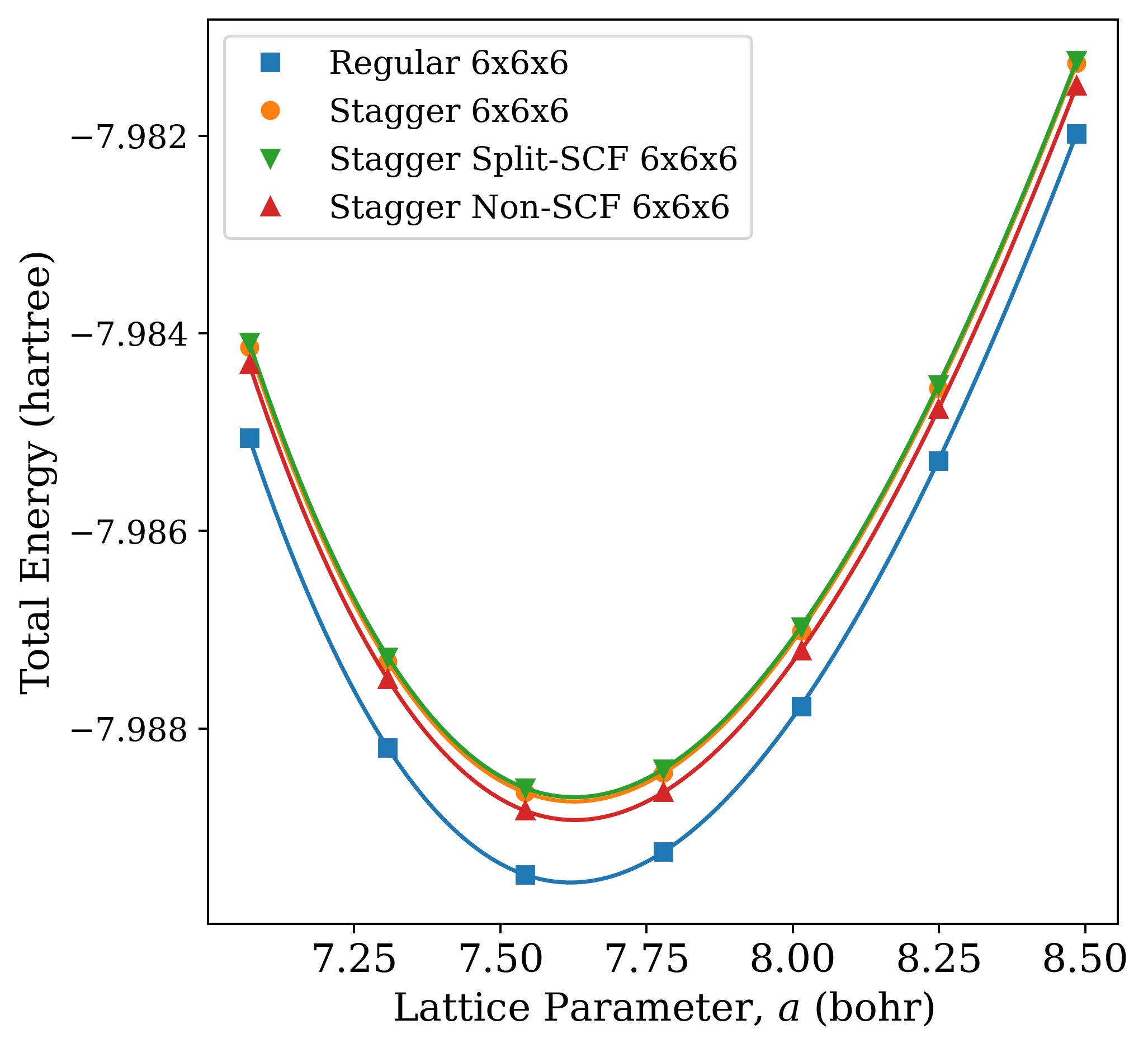
(a) LiH

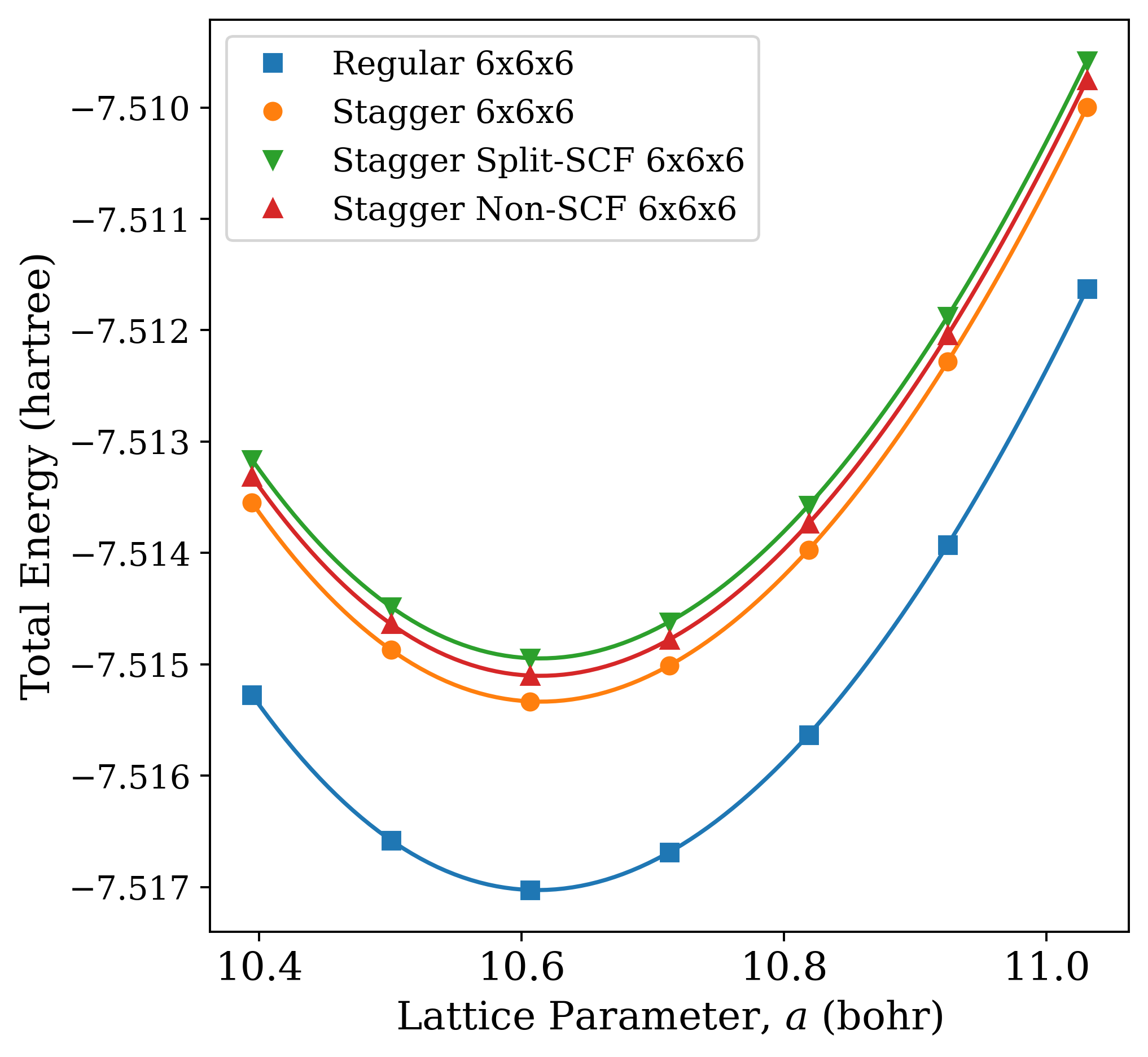
(b) Si

Figure 8: Birch-Murnaghan Fits

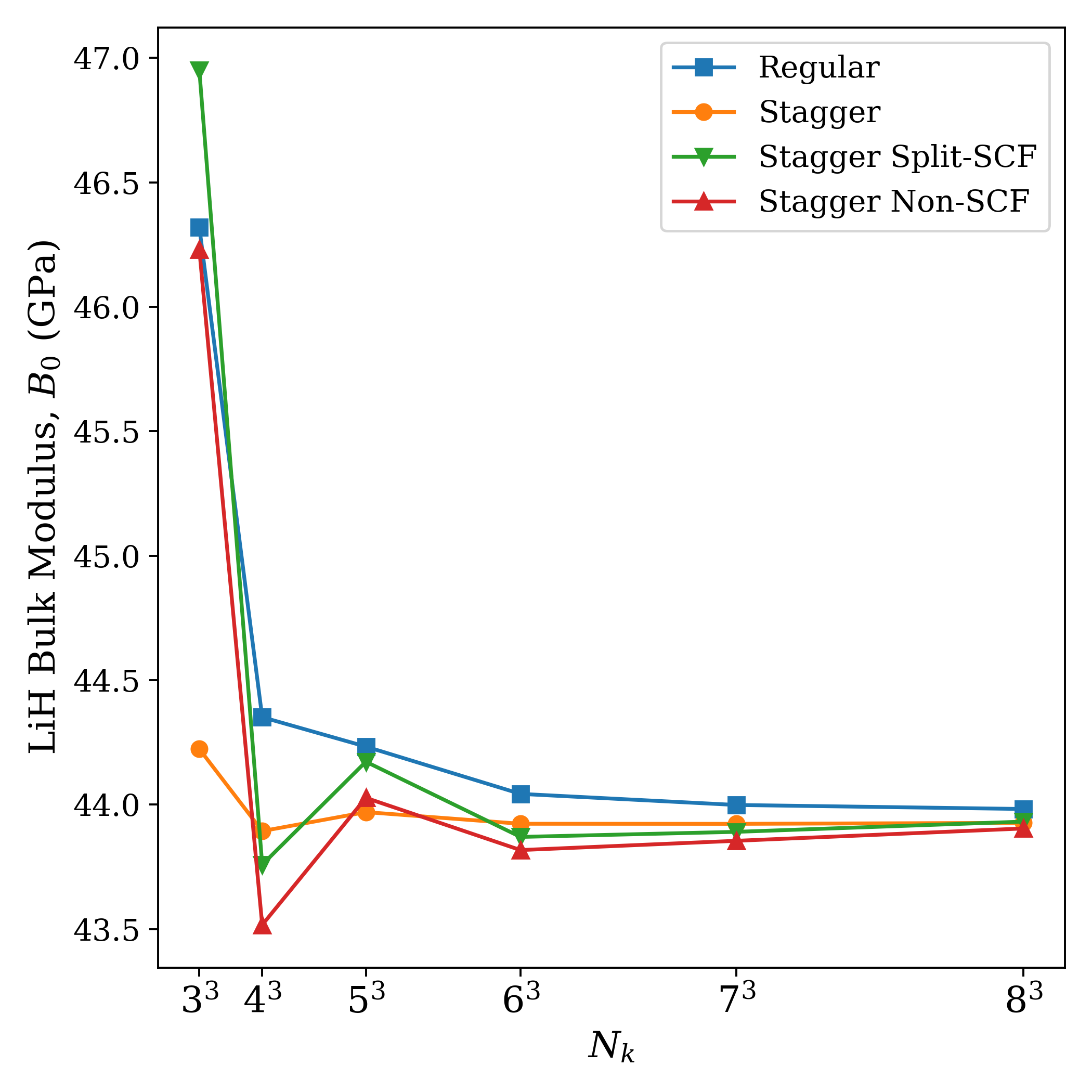
(a) LiH

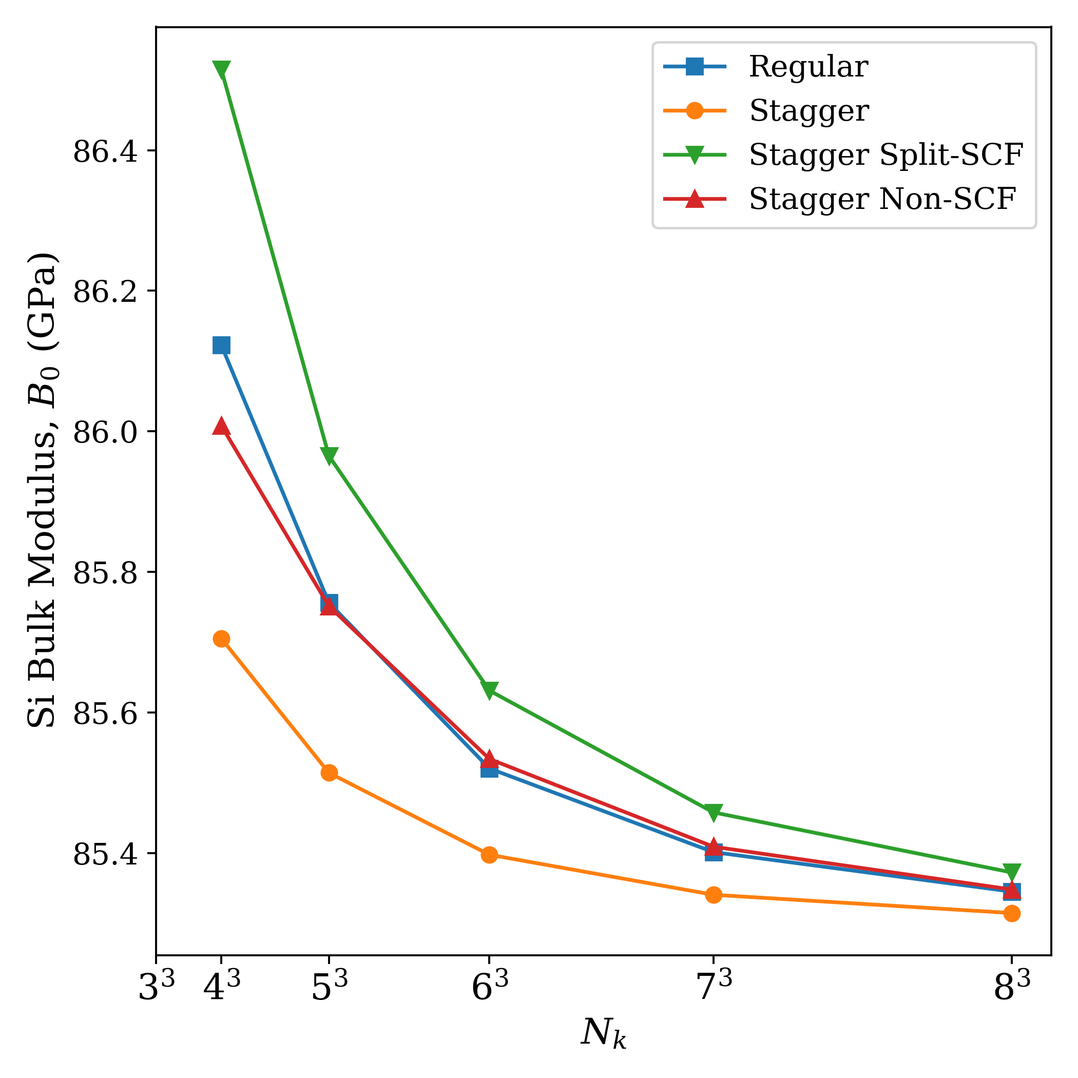
(b) Si

Figure 9: Finite Size Effects of Bulk Modulus

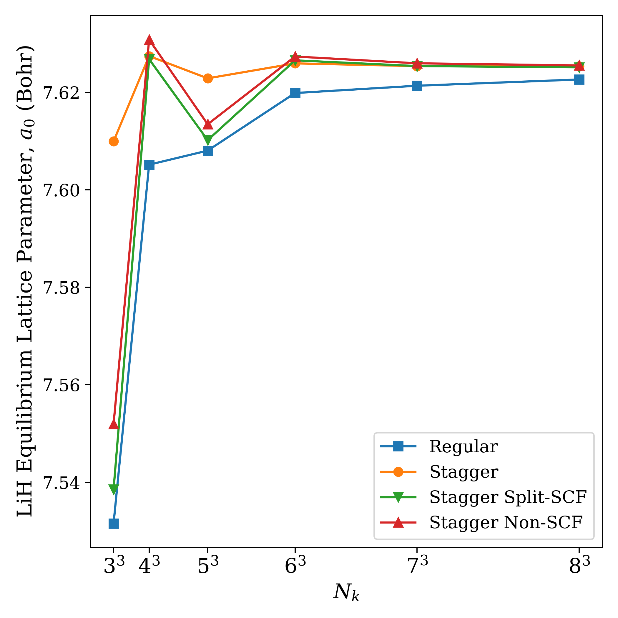
(a) LiH

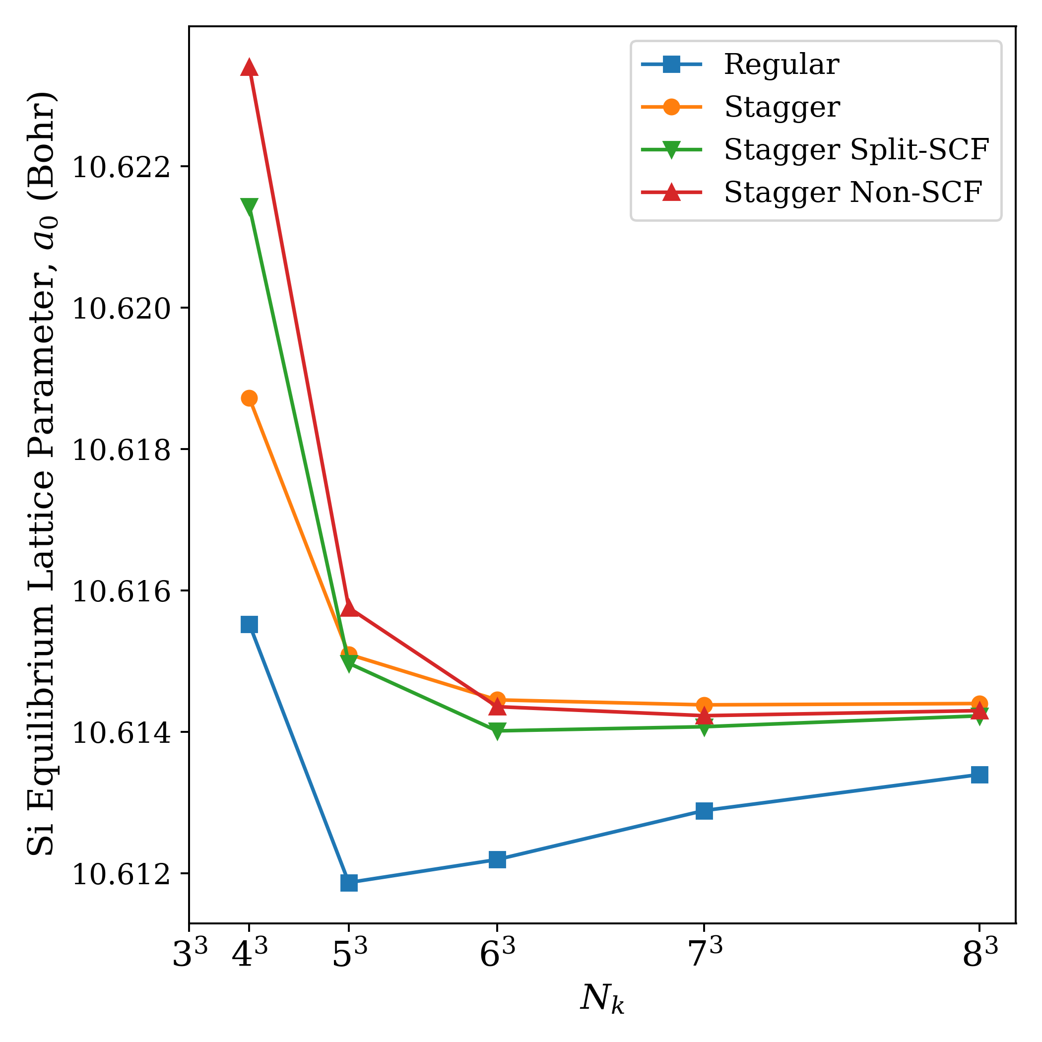
(b) Si

Figure 10: Finite Size Effects of Equilibrium Lattice Parameter

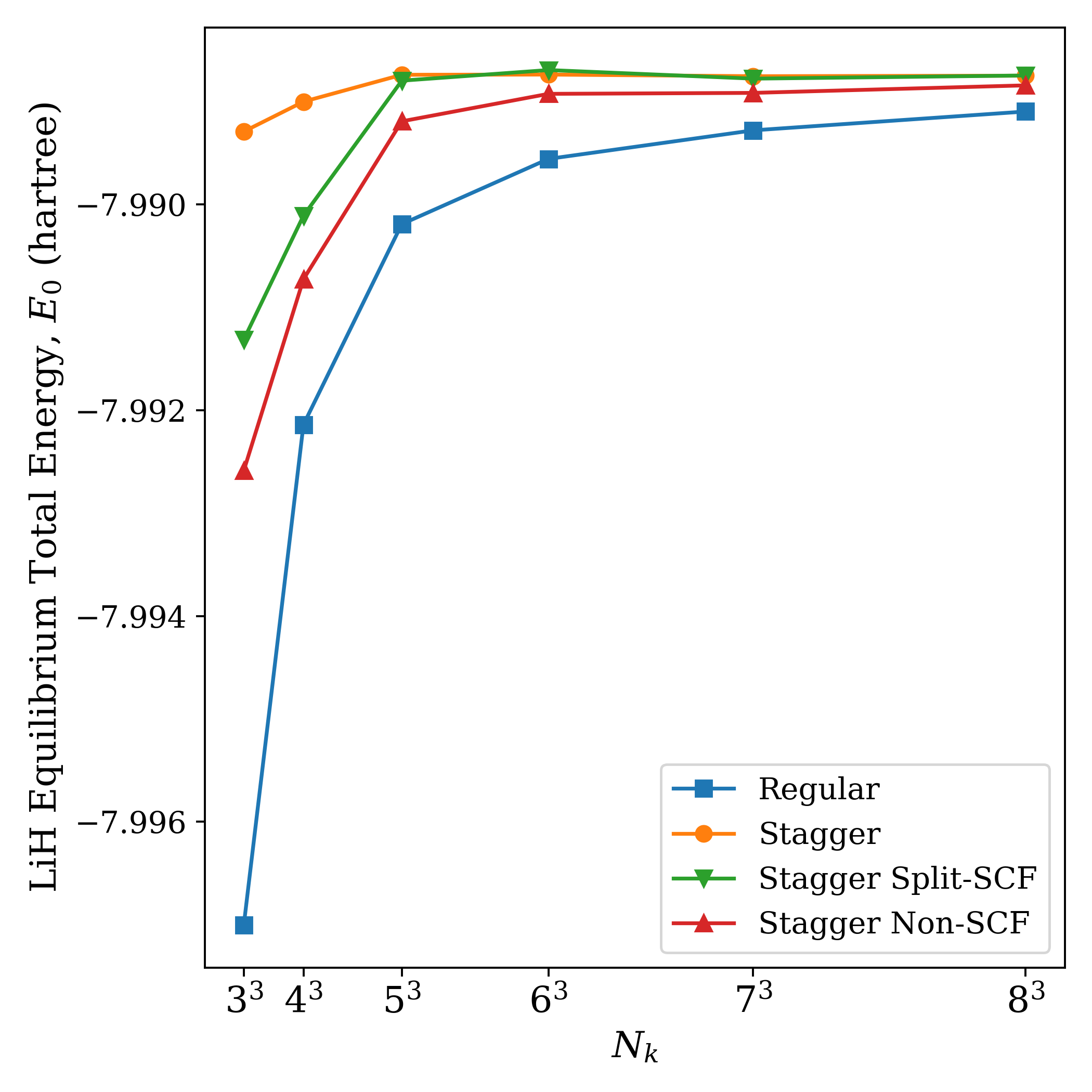
(a) LiH

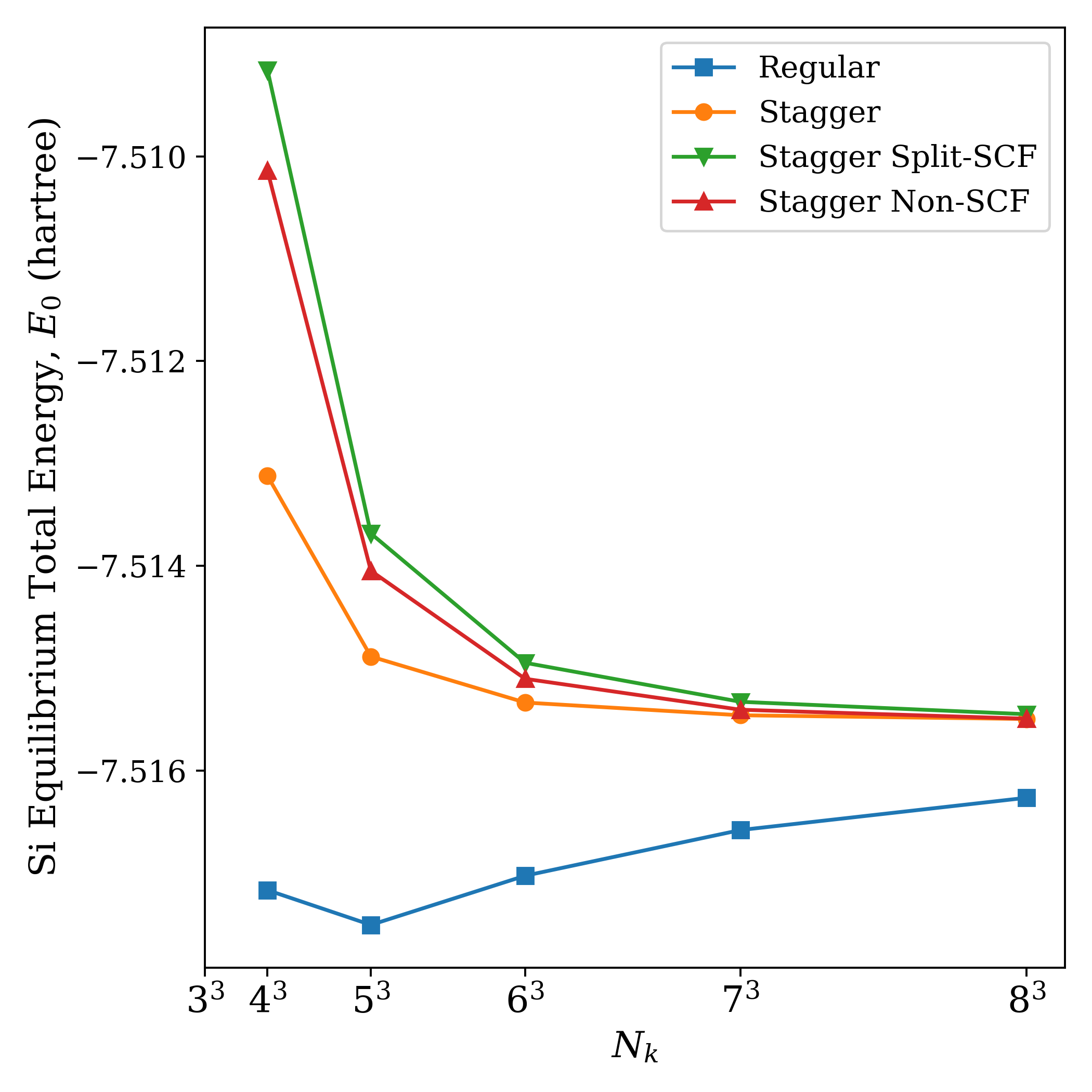
(b) Si

Figure 11: Finite Size Effects of Equilibrium Total Energy

Phase Transition Energies

The ability to predict the phase transition energy between two polymorphs of a material also presents a good test for the ability of the staggered mesh method to accurately recover measurable properties that are energy differences. For this study, we look at the transition (1) from diamond to rhombohedral graphite ^{35, 36, 37} and (2) from cubic to hexagonal BN ³⁸. The diamond-to-graphite transition shows a particularly marked improvement for the original staggered mesh method relative to the regular method. The other two staggered mesh variants, like the regular method, display severe oscillations towards the TDL. The original staggered mesh method attenuates such oscillations, which justifies its use of double $\mathbf{k}$-points compared to a normal calculation. For the cubic-to-hexagonal BN transition, all three staggered mesh methods perform similarly to each other, while the regular method appears to overshoot the TDL. Thus, just as shown in the convergence of the Burch-Murnaghan curves, all three versions of the staggered mesh method outperform the regular method, with the original version being the most suitable for these calculations.

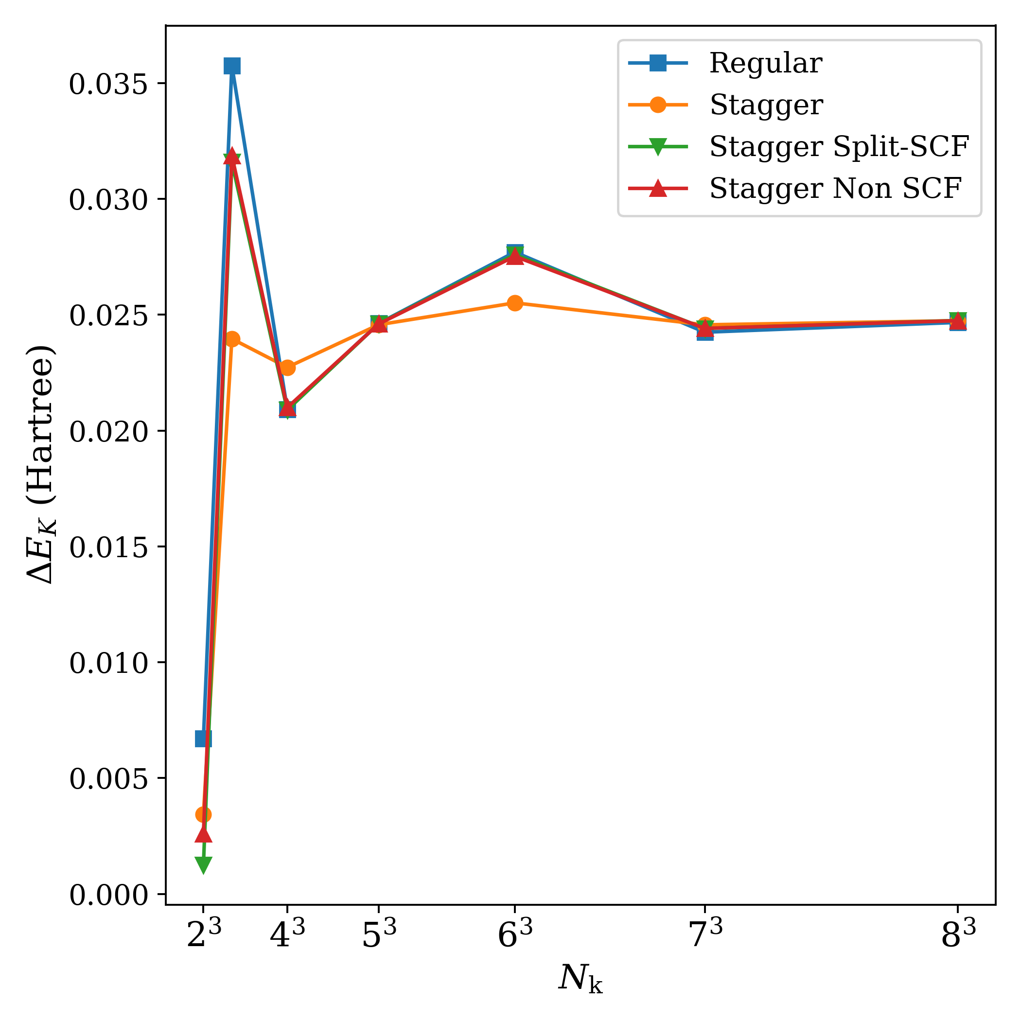
(a) Diamond to Graphite

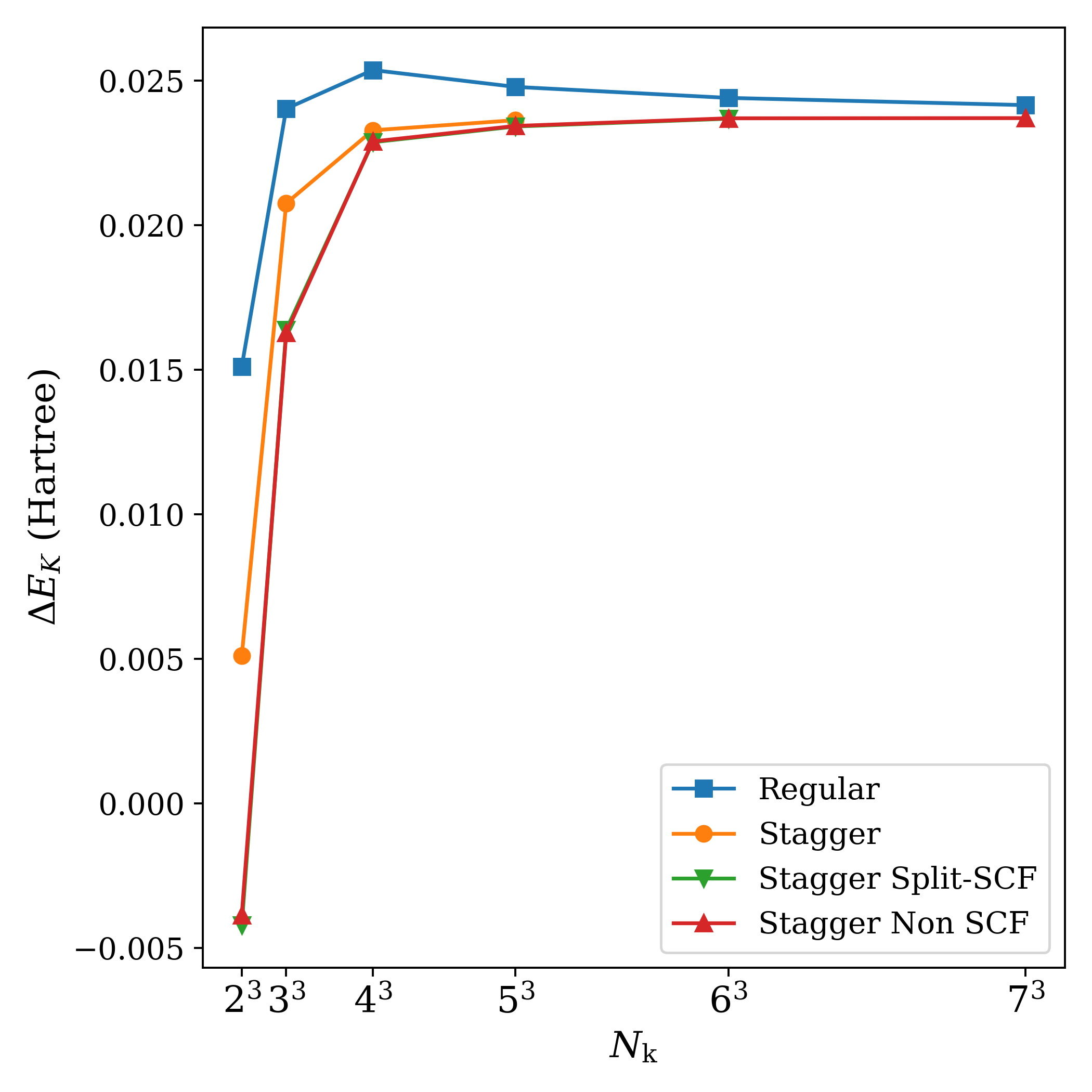
(b) Cubic to Hexagonal BN.

Figure 12: Finite size effects of phase transition energies. For Fig. 12(b), the incomplete data in the Stagger and Stagger Split-SCF lines is due to insufficient compute capabilities or SCF convergence issues.

Phonon Force Constants

We test the staggered mesh method’s ability to recover TDL potential energy surfaces (PES) around the equilibrium geometry for LiH and diamond. Specifically, by perturbing the atoms in the direction of a phonon, we can perform a quadratic fit of the total energy as a function of mode coordinate. For both LiH and diamond, we picked the highest frequency phonon at the $\Gamma$ point, which was verified by a Quantum Espresso calculation ³⁹ and the Phonon Visualizer by Materials Cloud ⁴⁰. For LiH, this corresponds to the oscillation of the H atom along the direction of a single lattice vector. We define a parametrized mode coordinate $\lambda$, so the phonon corresponds to [$\lambda$, 0.5, 0.5] in the basis of the rhombohedral primitive cell lattice vectors for LiH. Similarly, for diamond (which also has a rhombohedral primitive cell), we examine the mode corresponding to the oscillation of one of the carbon atoms along the direction of a lattice vector and define the parametrized coordinate of that atom as [$\lambda$, 0.25 0.25]. Subsequently, $\lambda=0.5$ and $\lambda=0.25$ represent the equilibrium positions for LiH and diamond respectively.

For the $6\times 6\times 6$ case, the PESs and their quadratic fits are shown in Fig. 13, while the convergence of the force constant with $N_{\textbf{k}}$ for each method is shown in Fig. 14 with their corresponding modes visualized. The original staggered mesh method shows improvement over its two other versions as well as the regular method, especially at low $N_{\textbf{k}}$. We note that for diamond specifically in Fig. 14(b), the force constant from the regular method may appear to be converging to a different TDL than those of the staggered mesh methods. This is because the regular method has slightly overshot the TDL value and is still increasing even at $N_{\textbf{k}}=8^{3}$. When comparing the staggered mesh methods the Split- and Non-SCF versions only begin to perform comparably to the original staggered mesh method at high $N_{\textbf{k}}$. Thus, despite its slightly higher cost, the original staggered mesh method shows the most promise in computing properties that are derivatives of the total energy, such as phonon force constants.

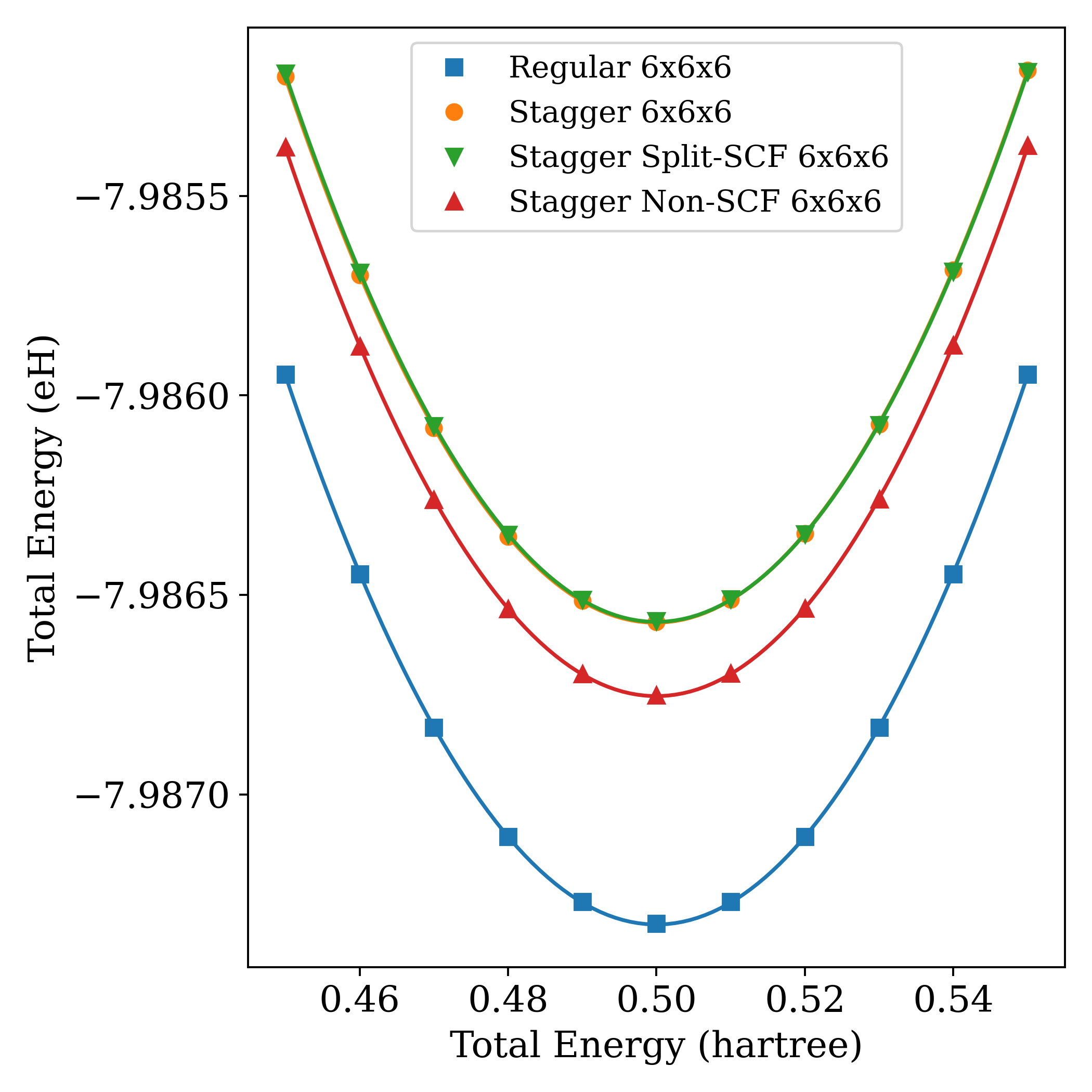
(a) LiH

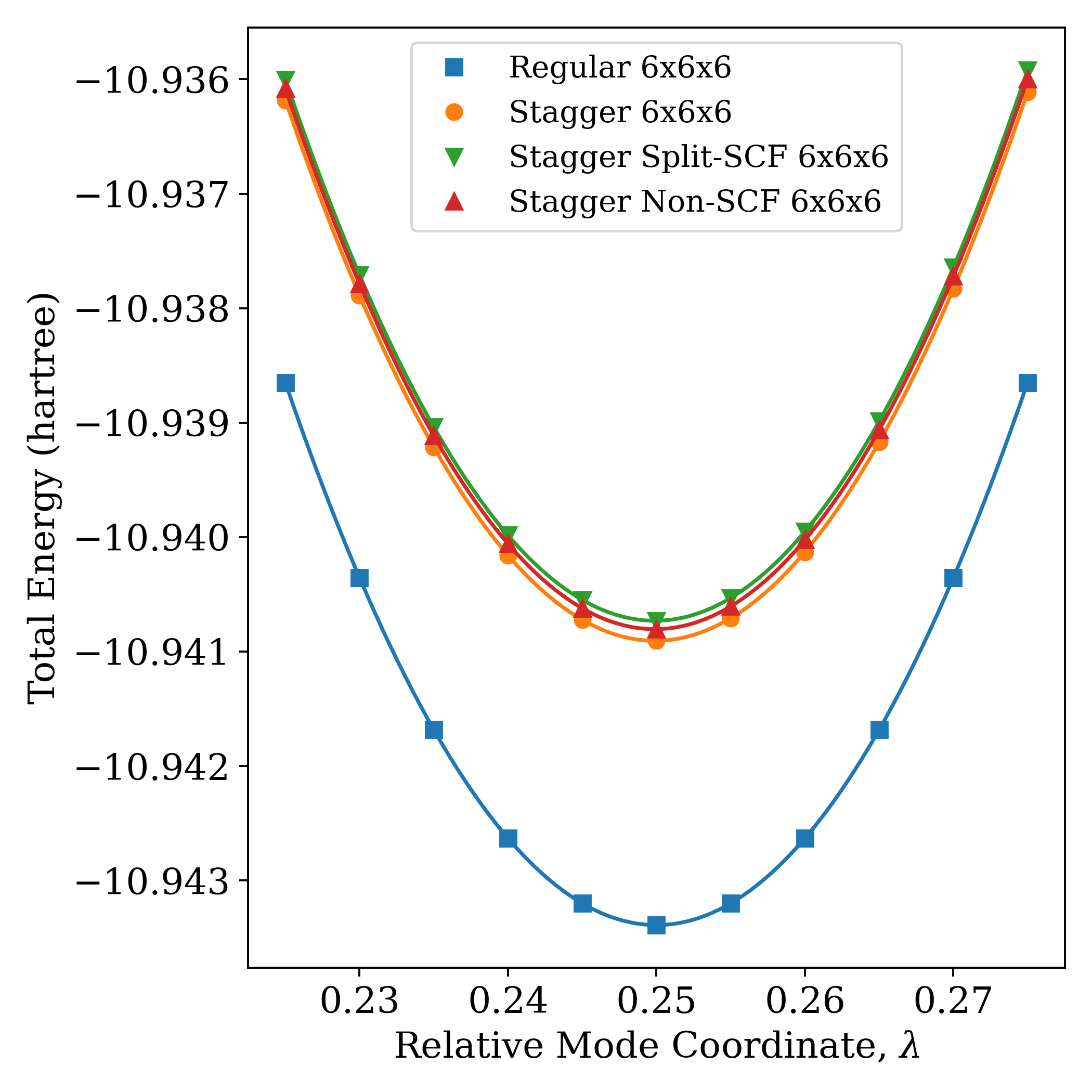
(b) Diamond

Figure 13: Energy Surfaces Recovered by the Regular and staggered mesh methods

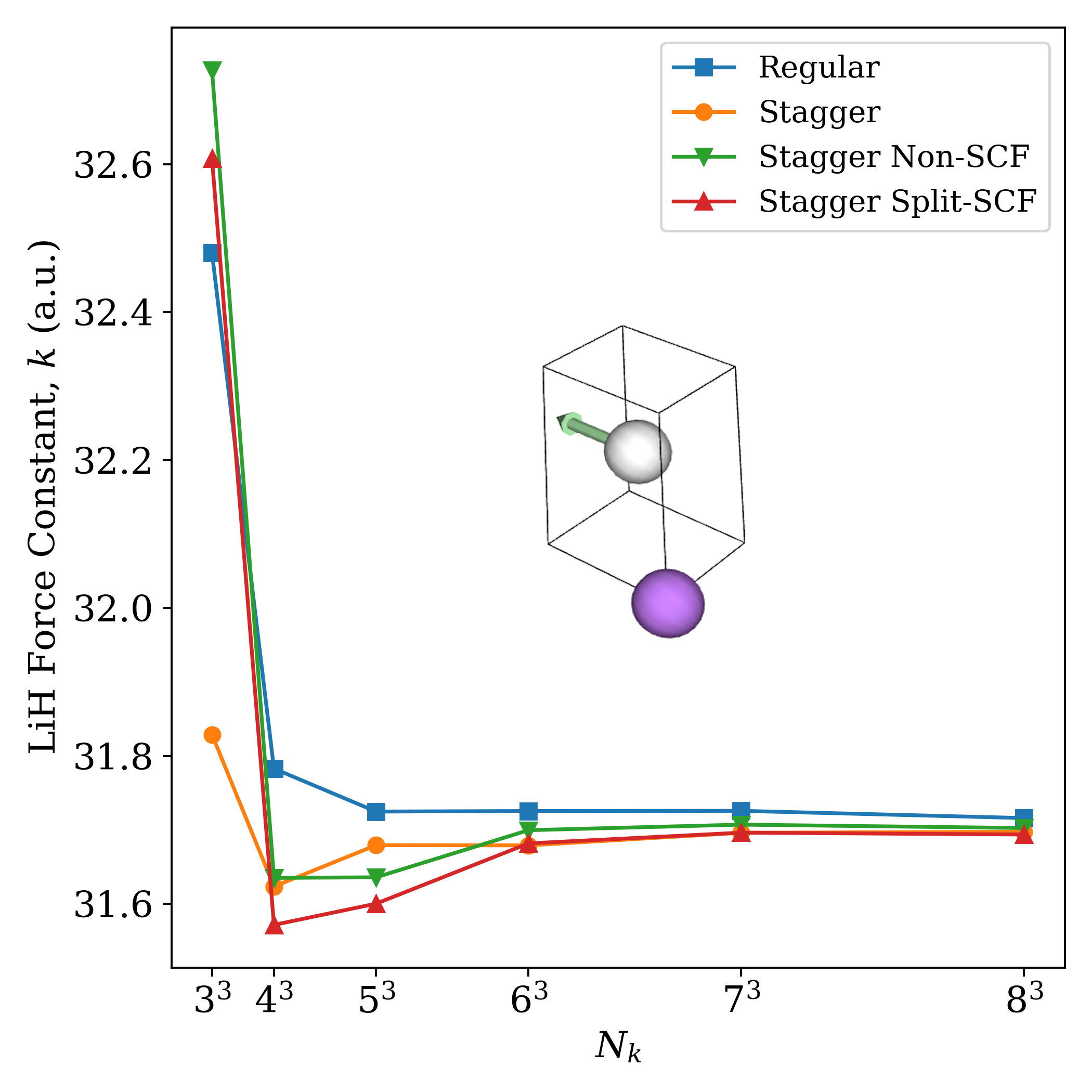
(a) LiH

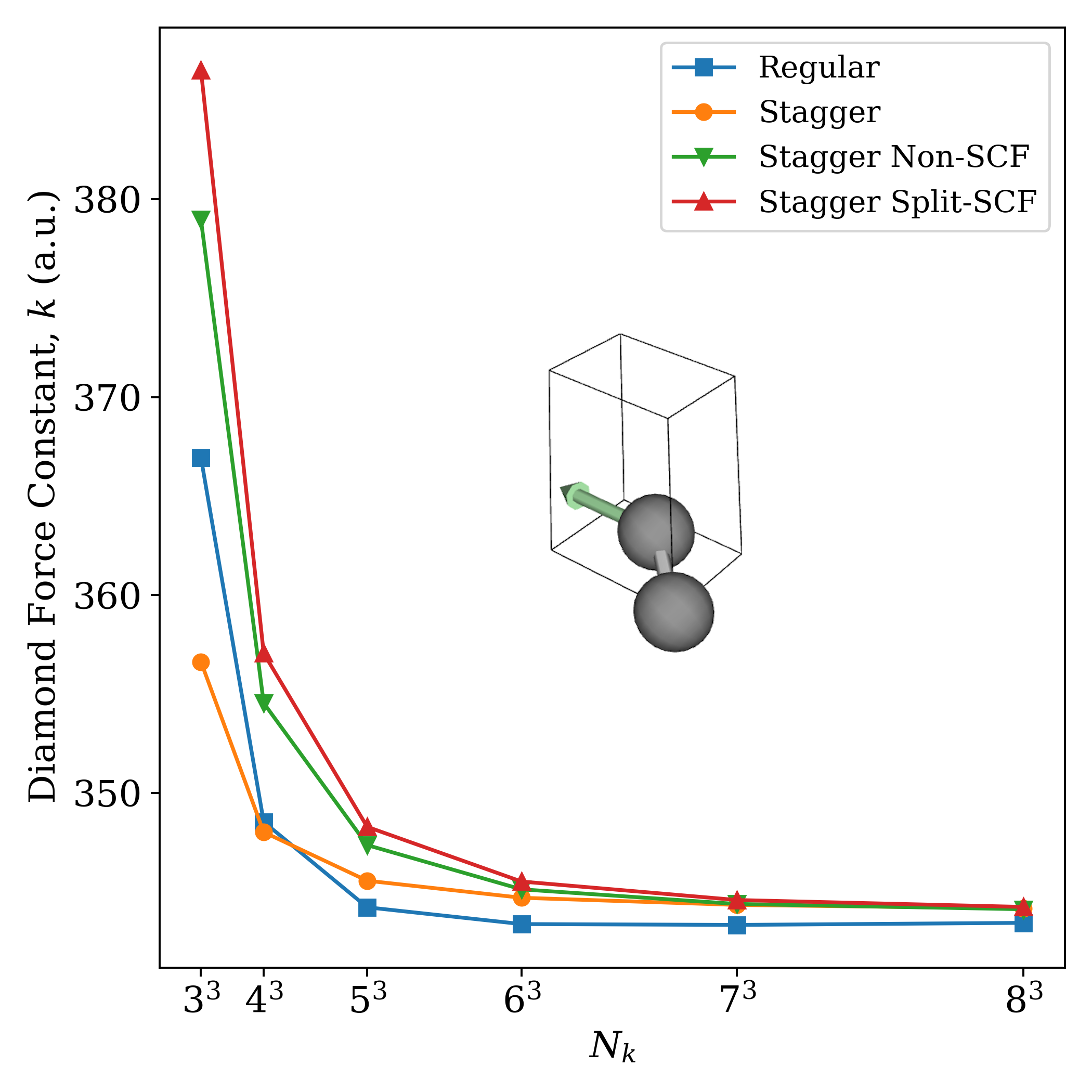
(b) Diamond

Figure 14: Force Constant Finite Size Effect

5 Discussion

The staggered mesh method presents a promising way to accelerate the convergence of the exact exchange energy towards the thermodynamic limit while requiring minimal modification to the SCF and band structure calculation procedures found in many solid-state quantum chemistry codes. It therefore has immediate applications in recovering more accurate energies obtained from using the increasingly popular hybrid functionals in periodic calculations. We also assessed the effectiveness of two other versions of the staggered mesh method designed to further reduce its cost: the Non-SCF and Split-SCF variants. We find that using staggered mesh Non-SCF recovers exchange energies and band gaps faster than the regular method as a function of $N_{\textbf{k}}$, at the cost of only an extra SCF cycle. In computing other properties of interest, including the bulk modulus, equilibrium lattice parameter, and equilibrium energy, the original version performs the best.

Beyond its utility in recovering more accurate energies, the staggered mesh method points to a new technique for reducing finite-size errors in periodic calculations by avoiding unnecessary singularities. Although this work discusses only the Hartree-Fock exchange energy, the energy gradients present a natural next step for testing the effectiveness of the staggered mesh method for a range of realistic systems. Staggered mesh techniques have also been developed for Second Order Moller-Plesset Perturbation theory (MP2) ¹⁹, coupled cluster, and random phase approximation (RPA) calculations²⁰. We also aim to extend the staggered mesh method to MP3 and its improved variants, in conjunction with acceleration techniques, such as tensor hypercontraction (THC) ⁴¹. While the present work primarily deals with 3D extended systems, studies on 2D (e.g. graphene, hexagonal BN) and 1D extended systems (polymers, nanotubes) ^{42, 43, 44, 45, 46} also present an opportunity for rigorous testing of the staggered mesh method in the wavefunction methods mentioned above.

This material is based upon work supported by the National Science Foundation Graduate Research Fellowship Program under Grant No. DGE 2146752 (SJQ) and the U.S. Department of Energy, Office of Science, Office of Advanced Scientific Computing Research and Office of Basic Energy Sciences, Scientific Discovery through Advanced Computing (SciDAC) program under Award Number DE-SC0022364 (LL, MHG). LL is a Simons Investigator in Mathematics.

Raw data for exchange energies, total energies, band gaps, Birch-Murnaghan fit data, and phonon data for the systems discussed in the work.

References

- Booth et al. 2013 Booth, G. H. et al. Towards an exact description of electronic wavefunctions in real solids. Nature 2013, 493, 365–370
- Raabe 2002 Raabe, D. Don’t trust your simulation - computational materials science on its way to maturity? Advanced Engineering Materials 2002, 4, 255–267
- Pisani et al. 2008 Pisani, C. et al. Periodic local MP2 method for the study of electronic correlation in crystals: Theory and preliminary applications. Journal of Computational Chemistry 2008, 29, 2113–2124
- Huang and Carter 2008 Huang, P.; Carter, E. A. Advances in correlated electronic structure methods for solids, surfaces, and nanostructures. Annual Review of Physical Chemistry 2008, 59, 261–290
- Jain et al. 2013 Jain, A. et al. Commentary: The Materials Project: A materials genome approach to accelerating materials innovation. APL Materials 2013, 1, 011002
- Monkhorst and Pack 1976 Monkhorst, H. J.; Pack, J. D. Special points for Brillouin-zone integrations. Phys. Rev. B 1976, 13, 5188–5192
- Xing et al. 2023 Xing, X.; Li, X.; Lin, L. Unified analysis of finite-size error for periodic Hartree-Fock and second order Møller-Plesset perturbation theory. Math. Comp. 2023,
- Fraser et al. 1996 Fraser, L. M. et al. Finite-size effects and Coulomb interactions in quantum Monte Carlo calculations for homogeneous systems with periodic boundary conditions. Phys. Rev. B 1996, 53, 1814–1832
- Drummond et al. 2008 Drummond, N. D. et al. Finite-size errors in continuum quantum Monte Carlo calculations. Phys. Rev. B 2008, 78, 125106
- Erba et al. 2023 Erba, A. et al. CRYSTAL23: a program for computational solid state physics and chemistry. J. Chem. Theory Comput. 2023, 19, 6891–6932
- Orlando et al. 2014 Orlando, R. et al. On the full exploitation of symmetry in periodic (as well as molecular) self-consistent-field ab initio calculations. The Journal of Chemical Physics 2014, 141, 104108
- Dovesi 1986 Dovesi, R. On the role of symmetry in the ab initio hartree-fock linear-combination-of-atomic-orbitals treatment of periodic systems. International Journal of Quantum Chemistry 1986, 29, 1755–1774
- Moreno and Soler 1992 Moreno, J.; Soler, J. M. Optimal meshes for integrals in real- and reciprocal-space unit cells. Phys. Rev. B 1992, 45, 13891–13898
- Morgan et al. 2018 Morgan, W. S. et al. Efficiency of Generalized Regular k-point grids. Computational Materials Science 2018, 153, 424–430
- Hart et al. 2019 Hart, G. L. W. et al. A robust algorithm for k-point grid generation and symmetry reduction. J. Phys. Commun. 2019, 3, 065009
- Spencer and Alavi 2008 Spencer, J.; Alavi, A. Efficient calculation of the exact exchange energy in periodic systems using a truncated Coulomb potential. Phys. Rev. B 2008, 77, 193110
- Schäfer et al. 2023 Schäfer, T. et al. Sampling the reciprocal Coulomb potential in finite and anisotropic cells. 2023; \urlhttp://arxiv.org/abs/2310.13608, arXiv:2310.13608 [physics]
- Bussy and Hutter 2024 Bussy, A.; Hutter, J. Efficient periodic resolution-of-the-identity Hartree–Fock exchange method with k-point sampling and Gaussian basis sets. The Journal of Chemical Physics 2024, 160, 064116
- Xing et al. 2021 Xing, X.; Li, X.; Lin, L. Staggered mesh method for correlation energy calculations of solids: second-order Møller–Plesset perturbation theory. J. Chem. Theory Comput. 2021, 17, 4733–4745
- Xing and Lin 2022 Xing, X.; Lin, L. Staggered mesh method for correlation energy calculations of solids: Random Phase Approximation in direct ring coupled cluster doubles and adiabatic connection formalisms. J. Chem. Theory Comput. 2022, 18, 763–775
- Guidon et al. 2009 Guidon, M.; Hutter, J.; VandeVondele, J. Robust periodic Hartree-Fock exchange for large-scale simulations using gaussian basis sets. J. Chem. Theory Comput. 2009, 5, 3010–3021
- mar 2004 Martin, R. M., Ed. Electronic Structure: Basic Theory and Practical Methods; Cambridge University Press: Cambridge, 2004; pp 499–511
- Hub et al. 2014 Hub, J. S. et al. Quantifying artifacts in Ewald simulations of inhomogeneous systems with a net charge. J. Chem. Theory Comput. 2014, 10, 381–390
- Paier et al. 2005 Paier, J. et al. The Perdew–Burke–Ernzerhof exchange-correlation functional applied to the G2-1 test set using a plane-wave basis set. The Journal of Chemical Physics 2005, 122, 234102
- Epifanovsky et al. 2021 Epifanovsky, E. et al. Software for the frontiers of quantum chemistry: An overview of developments in the Q-Chem 5 package. The Journal of Chemical Physics 2021, 155, 084801
- Jain et al. 2011 Jain, A. et al. A high-throughput infrastructure for density functional theory calculations. Computational Materials Science 2011, 50, 2295–2310
- Perdew et al. 1996 Perdew, J. P.; Burke, K.; Ernzerhof, M. Generalized gradient approximation made simple. Phys. Rev. Lett. 1996, 77, 3865–3868
- Dolgonos et al. 2019 Dolgonos, G. A.; Hoja, J.; Boese, A. D. Revised values for the X23 benchmark set of molecular crystals. Phys. Chem. Chem. Phys. 2019, 21, 24333–24344
- VandeVondele and Hutter 2007 VandeVondele, J.; Hutter, J. Gaussian basis sets for accurate calculations on molecular systems in gas and condensed phases. The Journal of Chemical Physics 2007, 127, 114105
- Lee et al. 2021 Lee, J. et al. Approaching the basis set limit in Gaussian-orbital-based periodic calculations with transferability: Performance of pure density functionals for simple semiconductors. J. Chem. Phys. 2021, 155, 164102, Publisher: American Institute of Physics
- Lippert et al. 1997 Lippert, G.; Hutter, J.; Parrinello, M. A hybrid Gaussian and plane wave density functional scheme. Molecular Physics 1997, 92, 477–488
- Kohn 1996 Kohn, W. Density functional and density matrix method scaling linearly with the number of atoms. Phys. Rev. Lett. 1996, 76, 3168–3171
- Birch 1947 Birch, F. Finite elastic strain of cubic crystals. Phys. Rev. 1947, 71, 809–824
- Sholl and Steckel 2009 Sholl, D. S.; Steckel, J. A. Density Functional Theory: A Practical Introduction, 1st ed.; Wiley, 2009
- Wen et al. 2006 Wen, B. et al. n-diamond: an intermediate state between rhombohedral graphite and diamond? New J. Phys. 2006, 8, 62
- Lipson and Stokes 1942 Lipson, H.; Stokes, A. R. The structure of graphite. Proceedings of the Royal Society of London. Series A, Mathematical and Physical Sciences 1942, 181, 101–105
- White et al. 2021 White, M. A. et al. The relative thermodynamic stability of diamond and graphite. Angewandte Chemie International Edition 2021, 60, 1546–1549
- Cazorla and Gould 2019 Cazorla, C.; Gould, T. Polymorphism of bulk boron nitride. Science Advances 2019, 5, eaau5832
- Giannozzi et al. 2017 Giannozzi, P. et al. Advanced capabilities for materials modelling with Quantum ESPRESSO. J. Phys.: Condens. Matter 2017, 29, 465901
- Talirz et al. 2020 Talirz, L. et al. Materials Cloud, a platform for open computational science. Sci Data 2020, 7, 299
- Bertels et al. 2019 Bertels, L. W.; Lee, J.; Head-Gordon, M. Third-order Møller–Plesset perturbation theory made useful? Choice of orbitals and scaling greatly improves accuracy for thermochemistry, kinetics, and intermolecular interactions. J. Phys. Chem. Lett. 2019, 10, 4170–4176
- Shanmugam et al. 2022 Shanmugam, V. et al. A review of the synthesis, properties, and applications of 2D materials. Particle & Particle Systems Characterization 2022, 39, 2200031
- Faulstich et al. 2023 Faulstich, F. M. et al. Interacting models for twisted bilayer graphene: A quantum chemistry approach. Phys. Rev. B 2023, 107, 235123
- Maschio 2018 Maschio, L. Direct inversion of the iterative subspace (DIIS) convergence accelerator for crystalline solids employing Gaussian basis sets. Theor Chem Acc 2018, 137, 60
- Ruipérez 2019 Ruipérez, F. Application of quantum chemical methods in polymer chemistry. International Reviews in Physical Chemistry 2019, 38, 343–403
- Kastinen et al. 2016 Kastinen, T. et al. Intrinsic properties of two benzodithiophene-based donor–acceptor copolymers used in organic solar cells: a quantum-chemical approach. J. Phys. Chem. A 2016, 120, 1051–1064