An Effective Incorporating Heterogeneous Knowledge Curriculum Learning for Sequence Labeling

Abstract

Sequence labeling models often benefit from incorporating external knowledge. However, this practice introduces data heterogeneity and complicates the model with additional modules, leading to increased expenses for training a high-performing model. To address this challenge, we propose a two-stage curriculum learning (TCL) framework specifically designed for sequence labeling tasks. The TCL framework enhances training by gradually introducing data instances from easy to hard, aiming to improve both performance and training speed. Furthermore, we explore different metrics for assessing the difficulty levels of sequence labeling tasks. Through extensive experimentation on six Chinese word segmentation (CWS) and Part-of-speech tagging (POS) datasets, we demonstrate the effectiveness of our model in enhancing the performance of sequence labeling models. Additionally, our analysis indicates that TCL accelerates training and alleviates the slow training problem associated with complex models.

Keywords: Curriculum Learning, Sequence Labeling, Difficulty Measure

1.   Introduction

Sequence labeling is a fundamental task in natural language processing (NLP) that involves assigning labels to individual elements in a sequence. Recent advancements in neural network approaches have demonstrated remarkable performance in sequence labeling tasks  Zhang et al. (2014); Chen et al. (2017); Zhang et al. (2018); Tian et al. (2020a); Nguyen et al. (2021); Hou et al. (2021); Liu et al. (2021). Some of these works have explored the integration of external knowledge, such as n-grams, lexicons, and syntax, to enhance sequence labeling models. However, this integration increases the heterogeneity and complexity of the input data. Furthermore, incorporating knowledge into sequence labeling models often requires additional encode modules, such as attention mechanisms  Liu et al. (2021); Tian et al. (2020a) or graph neural network (GNN) Gui et al. (2019); Nie et al. (2022). These additional modules increase the model’s parameters, making it more time-consuming and resource-intensive to develop a high-performing system.

Curriculum Learning (CL) is an effective approach to tackle these challenges  Bengio et al. (2009), as it mimics the human learning process by gradually introducing training samples from easy to hard, thereby enabling efficient learning in heterogeneous data while improving both the speed and quality of the model Wang et al. (2021). CL has demonstrated success in various NLP tasks, including machine translation Wan et al. (2020), dialogue generation Zhu et al. (2021), and text classification Zhang et al. (2022).

In CL, data-selection curriculum strategies play a crucial role. Recently,  Mohiuddin et al. (2022) proposed metrics that rely on the similarity of parallel sentence pairs to guide data selection in machine translation tasks. Similarly,  Yuan et al. (2022) introduced difficulty metrics for entity typing based on training loss. However, these difficulty metrics primarily focus on the sentence level, and there is a lack of token-level and word-level metrics to measure the difficulty of sequence labeling tasks.

To address this gap, in this paper, we introduce a two-stage curriculum learning (TCL) framework specifically designed for sequence labeling tasks. The first stage is data-level CL, where we train a basic teacher model on all available training data, aiming to alleviate the cold start problem of the student model. The second stage is model-level CL, where we start training the student model on a selected subset of the teacher model and gradually expand the training subset by considering the difficulty of the data and the state of the student model. Furthermore, we explore different difficulty metrics for sequence labeling tasks within the TCL framework. These metrics include a pre-defined metric, such as sentence length, and model-aware metrics, namely Top-N least confidence (TLC), Maximum normalized log-probability (MNLP), and Bayesian uncertainty (BU). Finally, we choose the classical sequence labeling tasks, Chinese word segmentation and part-of-speech tagging, to validate our proposed approach.

In summary, our work makes the following contributions:

• We propose a TCL framework for sequence labeling tasks. In the first stage, we train a simple transfer teacher model using all available data, which establishes the initial sample order for the student model and helps it warm up. In the second stage, we dynamically adjust the order of samples based on the current state of the student model.

• We design and compare various difficulty metrics tailored for sequence labeling tasks within the TCL framework. These metrics offer a more comprehensive assessment of the difficulty at the token and word levels, going beyond the traditional sentence-level metrics.

• We conduct extensive evaluations on six datasets encompassing sequence labeling tasks. Experiments and analyses show that our model accelerates training speed and the proposed difficulty metrics can plan more efficient learning paths for the model. Moreover, our approach exhibits flexibility and can be easily applied to other sequence labeling models.

2.   Related Work

In recent years, neural network methods have achieved remarkable success in sequence labeling tasks Zhang et al. (2014); Chen et al. (2017); Zhang et al. (2018); Gui et al. (2019); Tian et al. (2020a); Nguyen et al. (2021); Hou et al. (2021); Lobov et al. (2022). These studies commonly employ the fusion of external knowledge to enhance the performance of sequence labeling models. This external knowledge includes pre-trained embeddings Zhang et al. (2018); Shao et al. (2017), n-grams and lexicons Tian et al. (2020b); Liu et al. (2021), and syntax information Tian et al. (2020a); Tang et al. (2022). Specialized structures are employed to incorporate the knowledge, such as various variants of attention modules Liu et al. (2021); Tian et al. (2020a); Tang and Su (2022) and graph neural networks Gui et al. (2019); Huang et al. (2021); Tang et al. (2022). These structures effectively encode the relevant information from the input data. Nevertheless, their integration poses two challenges. Firstly, the inclusion of words, n-grams, and syntax information introduces heterogeneity and complexity to the input data. Secondly, the encoding modules increase the number of training parameters, making it more computationally expensive to train a model.

Curriculum learning (CL), introduced by Bengio et al. (2009), revolves around the principle of “training from easier data to harder data”. CL has been successfully applied to various NLP tasks, including machine translation Wan et al. (2020), dialogue generation Zhu et al. (2021), and text classification Zhang et al. (2022). It serves as an effective approach to address data heterogeneity and improve the performance of tasks.

The CL framework comprises two key components: difficulty measurement and training schedule. The former determines the relative “easiness” of each data example, which can be pre-defined or determined automatically. The latter determines the sequence of data subsets during the training process,guided by the judgment from the difficulty measurer Wang et al. (2021), using either a linear or non-linear scheduler. When both components are designed based on human prior knowledge, it is referred to as pre-defined CL. On the other hand, if one of the components is driven by a data-driven algorithm, it is known as automatic CL, exemplified by self-paced learning and transfer teacher. Pre-defined difficulty measurer is typically designed by considering data characteristics such as sentence length and word rarity. In general, designing difficulty metrics specifically tailored to the task at hand is more efficient and typically involves data-driven algorithms. For instance,  Mohiuddin et al. (2022) developed three deterministic scoring methods for machine translation that leverage the similarity of a parallel sentence pairs and cross-entropy.  Zhu et al. (2021) evaluated sample difficulty in dialogue generation based on model loss.  Lobov et al. (2022) utilized metrics such as sentence length, average confidence, and perplexity value to assess difficulty in named entity recognition (NER). However, these metrics primarily concentrate on the sentence-level and do not adequately address token- and word-level difficulty.

3.   Method

The framework proposed in this study consists of three main components: a teacher sequence labeling model, a student sequence labeling model, and a TCL training strategy. It is worth noting that the TCL is independent of the sequence labeling model. In line with previous studies, we adopt an encoder-to-decoder framework for the sequence labeling model, where the encoder is typically a pre-trained language model (PLM), and the decoder can be either a conditional random field (CRF) layer or a Softmax layer. Figure 1 illustrates the overall architecture of the proposed model.

Following previous works Zhang et al. (2018); Gong et al. (2019); Fu et al. (2020), in sequence labeling tasks, we feed an input sentence $X=\{x_{1},...x_{i}...,x_{M}\}$ into the encoder, and the decoder then outputs a label sequence $Y^{*}=\{y_{1}^{*},...y_{i}^{*}...y_{M}^{*}\}$, where $y_{i}^{*}$ represents a label from a pre-defined label set $T$, and $M$ denotes the length of sentence.

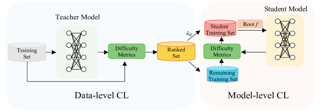
Figure 1: The framework of the proposed model consists of a teacher model, a student model, and a TCL strategy. Here, “Root f” represents Root function.

3.1.   Two-stage Curriculum Learning

Algorithm 1 Training Process

1:Original corpus D, difficulty metric $S(\cdot)$, training epochs of the teacher model $E_{0}$, training epochs of the student model $E_{s}$, training scheduler $\lambda$, length function $|\cdot|$.

2:A trained student model $\theta$

3:// data level curriculum learning

4:Train the teacher model $\theta_{0}$ with D for $E_{0}$ epochs

5:Get $S(\theta_{0})$ for each sample in D

6:Rank samples in D based on $S(\theta_{0})$ from small to large to get $\textit{D}_{r}$

7:// model level curriculum learning

8:Initial size of the training set of the student model: $m=\lambda|D|$

9:Initial training set for the student model: $D_{s}=D_{r}[0:m]$

10:The remaining training data: ${D}_{o}={D}_{r}[m:]$

11:for $epoch=1,2,..E_{s}$ do

12:     if  $\lambda$ <1 then

13:         a) Train the student model on $\textit{D}_{s}$ get

14:         current model $\theta_{*}$

15:         b) Get $S(\theta_{*})$ for each sample in $\textit{D}_{o}$

16:         c) Rank samples in $\textit{D}_{o}$ based on

17:         $S(\theta_{*})$ from small to large to get $\textit{D}_{r}$

18:         d) Update $\lambda$

19:         e) Obtain the number of new training

20:         data: $m=\lambda|D|-|D_{s}|$

21:         f) Add new training data into the

22:         student training set: ${D}_{s}+={D}_{r}[0:m]$

23:         g) The remaining data: ${D}_{o}={D}_{r}[m:]$

24:     else

25:         Train the student model on $\textit{D}_{s}$

26:     end if

27:end for

We present a novel two-stage curriculum learning approach: data-level CL and model-level CL. The Algorithm 1 provides a detailed explanation of the process.

At the data level, the algorithm begins by training a basic transfer teacher model on the entire training dataset $D$ for a specified number of epochs ($E_{0}$) to obtain the teacher model parameter $\theta_{0}$ (Line 1). It is worth noting that $E_{0}$ is selected to be smaller than the total number of epochs required for achieving convergence.

Next, the algorithm utilizes the teacher model $\theta_{0}$ to calculate a difficulty score $S(\theta_{0})$ for each sample in the training dataset $D$ (Line 2). These samples in D are then sorted in ascending order based on their difficulty scores, resulting in a newly organized dataset $\textit{D}_{r}$ (Line 3).

At the model level, the algorithm addresses the cold-start problem by initializing the training set of the student model, denoted as $D_{s}$, with a certain percentage of samples from $D_{r}$ (Line 4-5). The parameter $\lambda$ represents the proportion of these samples and plays a crucial role in controlling the curriculum learning process. The remaining data in $D_{r}$ that is not included in $D_{s}$ is represented as $D_{o}$ (Line 6). Gradually, the algorithm incorporates the samples from $D_{o}$ into $D_{s}$ by adjusting the threshold parameter $\lambda$. In the algorithm, we denote the number of new data to be added by $m$, and the value of $m$ is determined by $\lambda$ (Line 4, 15-16).

Next, we describe the update process of $D_{s}$. In the algorithm, the student model is initially trained on $D_{s}$ to obtain the updated model parameter $\theta_{*}$ (Line 9-10). The remaining data $D_{o}$ is then ranked according to the difficulty metric $S(\theta)$, resulting in a new ranked dataset $D_{r}$ (Line 11-13).

The algorithm proceeds to update the threshold parameter $\lambda$ (line 14) and calculates the number of new training samples to be added to the student training set $D_{s}$ from $D_{r}$ based on this parameter (lines 15-19). This process gradually incorporates new and more challenging samples into the student model training set. Consequently, as $\lambda$ reaches 1, all the data in $D_{o}$ is incorporated into $D_{s}$. Finally, the complete dataset is used to train the student model until convergence is achieved.

In algorithm 1, two crucial components play a significant role: the difficulty metrics $S(\cdot)$ and the threshold $\lambda$. These elements control the difficulty ranking of training samples and the progression of training samples feeding into the model, respectively. In the following sections, we will describe the design of each of these two elements.

3.2.   Difficulty Metrics

In sequence labeling tasks, the difficulty of samples is intricately associated with each token in the sequence. However, since it is difficult to assess the difficulty of individual tokens, we draw on the concept of uncertainty commonly used in active learning to reflect the difficulty of the samples, which quantifies whether the current model is confident or hesitant in labeling the training samples. In short, if the model is confident in predicting a sample, it is considered an easy sample. Therefore, the difficulty of the sample is dynamically evaluated based on the model capacity.

Next, we provide detailed formulations of various strategies for computing the difficulty $S(\cdot)$ in Algorithm 1.

Top-N least confidence (TLC). Culotta and McCallum (2005) proposed a confidence-based strategy for sequence models called least confidence (LC). This approach sorts the samples in ascending order based on the probability of the most possible label predicted by the model.

The least confidence of each token is calculated as follows.

$$\phi_{(x_{i},\theta)}^{LC}=1-max_{y_{i}\in T}P(y_{i}|x_{i})$$ (1)

where $x_{i}$ is the $i_{th}$ token in the input sentence, $\theta$ denotes model parameters, $y_{i}$ is a pre-defined label, $T$ represents the pre-defined label set. $max_{y_{i}\in T}P(y_{i}|x_{i})$ aims to find the probability of the most possible label predicted by the model. The smaller $\phi_{(x_{i},\theta)}^{LC}$ reflects the more confident the model is in predicting the label of $x_{i}$.

According to Agrawal et al. (2021), the confidence level of a sentence in a sequence labeling task is typically determined based on a set of representative tokens. Therefore, we select the top $N$ tokens with the highest least confidence in the sentence and then use their average value as the difficulty score of the sentence. Finally, the TLC difficulty metric is formulated as follows.

Maximum normalized log-probability (MNLP). Shen et al. (2018) used MNLP as a confidence strategy to find the product of the maximum probabilities of each token, which is equivalent to taking the logarithm of each probability and summing them. Finally, it is normalized to obtain the confidence score of the sentence as follows.

$$\prod_{i=1}^{M}max_{y_{i}\in T}P(y_{i}|x_{i})\Longleftrightarrow$$ (3)

$$\sum_{i=1}^{M}log\{max_{y_{i}\in T}P(y_{i}|x_{i})\}$$

where $M$ is the length of the sentence. The difficulty of a sentence decreases as the confidence level increases. To account for this relationship, we introduce a negative sign. Additionally, in order to reduce the impact of sentence length, we apply a normalization operation. Finally, MNLP is formulated as follows.

Bayesian uncertainty (BU). Buntine and Weigend (1991) proposed that model uncertainty can be assessed by the Bayesian Neural network. According to Wang et al. (2019), the higher predicted probability variance reflects the higher uncertainty that the model has with respect to the sample. Thus, if the model has a large variance in the predicted probability of the sample, the sample is difficult, and vice versa. In this work, we employ the widely used Monte Carlo dropout Gal and Ghahramani (2016) to approximate Bayesian inference.

First, we use Monte Carlo dropout Gal and Ghahramani (2016) to obtain samples of token-level tagging probabilities. We perform $K$ times prediction for each sample in the training set to obtain ${P(y_{i}|x_{i})}_{1}$,…, ${P(y_{i}|x_{i})}_{K}$. Then the expectation of token-level tagging probability can be approximated by

The variance of token-level tagging probability on the label set can be approximated by

$$var(x_{i},\theta)\approx$$ (6)

$$\leavevmode\resizebox{399.2946pt}{}{$\sum_{y_{i}\in T}(\frac{1}{K}\sum_{k=1}^{K}{P(y_{i}|x_{i})}_{k}^{2}-\{\mathbb{E}[P(y_{i}|x_{i})]\}^{2})$}$$

Now, we obtain the variance of each token $var(x_{i},\theta)$, then we use the average variance score of all tokens in the sequence as the sentence-level variance as follows.

The maximum variance score $var(\theta)_{max}$ also is valuable, which reflects the highest uncertainty in the sequence.

$$var(\theta)_{max}=max_{i\in[0,M]}var(x_{i},\theta)$$ (8)

The final uncertainty score or difficulty score of each sequence is calculated as follows.

$$S(\theta)^{BU}=var(\theta)_{max}+var(\theta)_{aver.}$$ (9)

Both at the data level and model level, the difficulty of training samples is measured by the above various $S(\theta)$.

3.3.   Training Scheduler

The training scheduler controls the pace of CL. In our work, we use the Root function as the control function, which allocates ample time for the model to learn newly added examples while gradually reducing the number of newly added examples during the training process.

$$\lambda\ =\ min(1,\sqrt{\frac{1-\lambda_{0}^{2}}{E_{grow}}\cdot E_{s}+\lambda_{0}^{2}})$$ (10)

where $E_{grow}$ represents the number of epochs at which $\lambda$ first reaches 1. Here, $\lambda_{0}>0$ denotes the initial proportion of the easiest training samples, and $E_{s}$ represents the number of training epochs. When $\lambda$ reaches 1, it indicates the model can use the entire training set.

4.   Experiments

4.1.   Dataset and Experimental Configurations

Chinese word segmentation (CWS) and part-of-speech (POS) tagging are representative sequence labeling tasks. So we evaluate our approach using six CWS and POS tagging datasets, including Chinese Penn Treebank version 5.0, 6.0, and 9.0, as well as the Chinese portion of Universal Dependencies(UD) and PKU  Jin and Chen (2008). Since the data in the UD dataset is in traditional Chinese, we converted it to simplified Chinese. Regarding the CTB datasets, we follow the same approach as previous works Shao et al. (2017); Tian et al. (2020a) by splitting the data into train/dev/test sets. In the case of PKU, We randomly select 10% of the training data to create the development set. For the UD dataset, we used the official splits of the train/dev/test sets. It is important to note that the UD dataset has two versions: UD1, which consists of 15 POS tags, and UD2, which includes 42 POS tags. The details of the six datasets are given in Table 1.

Datasets		CTB5	CTB6	CTB9	UD1	UD2	PKU
Train	Sent.	18k	23K	106k	4k	4k	17k
	Word	494k	641	1696k	99k	99k	482k
Dev	Sent.	350	2K	10k	500	500	1.9k
	Word	7k	60K	136k	13k	13k	53k
Test	Sent.	348	3K	16k	500	500	3.6k
	Word	8k	82K	242k	12k	12k	97k

Table 1: Detail of the six datasets.

Various methods have shown significant progress in fine-tuning Pretrained Language Models (PLM) for sequence labeling tasks Tian et al. (2020a, b); Liu et al. (2021). In this study, we use BERT-based Devlin et al. (2019) and RoBERTa-based Liu et al. (2019) models as encoders, following their default settings. According to Qiu et al. (2020), there is little difference in the decoding effects between Softmax and Conditional Random Fields (CRF) for sequence labeling tasks. Consequently, we opt for Softmax as the decoder. The framework of the basic transfer teacher is BERT+Softmax. As for the student model, we choose two simpler models (BERT/RoBERTa+Softmax) and two representative complex models introduced by  Tian et al. (2020a) and  Tang et al. (2023). In their work,  Tian et al. (2020a) employed a two-way attention mechanism, known as MCATT, to integrate dependency relations, POS labels, and syntactic constituents for the joint CWS and POS tagging task. They employed BERT as the encoder for this setup. On the other hand,  Tang et al. (2023) incorporated syntax and semantic knowledge into sequence labeling tasks using a GCN module called SynSemGCN. They applied RoBERTa as the sequence encoder in their experiment.

The values of $\lambda_{0}$ and $E_{grow}$ in Eq. 10 are set to 0.3 and 10, respectively. For the TLC difficulty metric, the key hyperparameter $N$ is set to 5. For the BU difficulty metric, the key hyperparameter $K$ is set to 3. The number of training epochs for the teacher model denoted as $E_{0}$, is set to 5. For further details on the important hyper-parameters of the model, please refer to Table 2.

Curriculum Learning Baselines. There are two baseline difficulty metrics for curriculum Learning: a. Random, which assigns samples in a random order; b. Sentence length (Length), which ranks samples from shortest to longest based on the intuition that longer sequences are more challenging to encode.

Hyper-parameters
$E_{0}$	5
$E_{s}$	50
$\lambda_{0}$	0.3
$E_{grow}$	10
$K$	3
$N$	5

Table 2: Experiment hyper-parameters setting.

Model					TCL Setting	CTB5		CTB6		CTB9		UD1		UD2	PKU
		CWS	POS	CWS	POS	CWS	POS	CWS	POS	CWS	POS	CWS	POS
BERT	NA	98.49	96.34	97.29	94.71	97.53	94.61	98.20	95.70	98.25	95.33	98.01	95.49
	Random	98.77	96.80	97.35	94.83	97.35	94.71	98.26	95.74	98.32	95.51	98.32	96.30
	Length	98.88	96.81	97.44	94.88	97.75	95.03	98.34	95.94	98.27	95.35	98.40	96.29
	TLC	98.71	96.85	97.41	94.91	97.74	94.99	98.30	95.81	98.25	95.47	98.40	96.33
	MNLP	98.90	96.99	97.40	94.92	97.74	95.01	98.27	95.78	98.30	95.58	98.40	96.31
	BU	98.84	96.80	97.45	94.92	97.75	95.00	98.28	95.84	98.32	95.60	98.41	96.32
RoBERTa	NA	98.66	96.50	97.31	94.80	97.58	94.70	98.25	95.80	98.17	95.32	98.30	95.85
	Random	98.70	96.75	97.48	94.90	97.33	94.23	98.34	95.82	98.23	95.42	98.51	96.51
	Length	98.73	96.73	97.42	94.91	97.77	95.09	98.26	95.80	98.25	95.47	98.53	96.47
	TLC	98.79	96.86	97.41	94.98	97.75	95.03	98.32	95.91	98.20	95.52	98.63	96.50
	MNLP	98.72	96.85	97.47	95.06	97.74	95.07	98.23	95.78	98.30	95.50	98.51	96.54
	BU	98.77	96.80	97.42	95.00	97.77	95.09	98.21	95.85	98.29	95.60	98.54	96.50
MCATT	NA	97.72	96.55	97.39	94.80	97.28	93.92	98.28	95.70	98.28	95.40	98.20	96.25
	Random	98.81	96.84	97.37	94.90	97.13	93.83	98.25	95.61	98.31	95.47	98.38	96.27
	Length	98.83	96.85	97.35	94.82	97.60	94.71	98.23	95.66	98.34	95.61	98.40	96.25
	TLC	98.83	96.89	97.37	94.83	97.60	94.68	98.33	95.61	98.15	95.53	98.41	96.30
	MNLP	98.85	96.81	97.41	94.92	97.64	94.70	98.42	95.87	98.26	95.35	98.41	96.30
	BU	98.91	96.87	97.42	94.90	97.69	94.88	98.34	95.66	98.18	95.49	98.43	96.32
SynSemGCN	NA	98.75	96.73	97.89	94.95	97.70	94.91	98.24	95.93	98.21	95.51	98.37	96.17
	Random	98.84	97.86	97.99	95.05	97.50	94.54	98.25	95.85	98.22	95.44	98.48	96.40
	Length	98.80	96.84	97.40	94.94	98.01	95.54	98.22	95.89	98.24	95.57	98.53	96.48
	TLC	98.83	97.81	97.98	95.02	98.00	95.53	98.36	95.99	98.28	95.50	98.61	96.55
	MNLP	98.78	97.72	98.04	95.13	98.02	95.53	98.26	95.89	98.30	95.61	98.56	96.48
	BU	98.90	97.95	98.05	95.14	98.03	95.48	98.34	96.06	98.23	95.48	98.59	96.54

Table 3: Experimental results of different models using different TCL settings on test sets of six datasets. SynSemGCN represents the model from Tang et al. (2023) and MCATT denotes the model from Tian et al. (2020b). Here, “CWS” represents the F1 value of CWS, and “POS” means the F1 value of the joint CWS and POS tagging. “NA” means without the TCL training strategy. The maximum F1 scores for each dataset are highlighted.

Model				CTB5		CTB6		CTB9		UD1		UD2	PKU
	CWS	POS	CWS	POS	CWS	POS	CWS	POS	CWS	POS	CWS	POS
Chen et al. (2017)	-	93.19	-	-	-	-	-	-	-	-	-	90.16
Shao et al. (2017)	98.02	94.38	-	-	96.67	92.34	95.16	89.75	95.09	89.42	-	-
Zhang et al. (2018)	98.50	94.95	96.36	92.51	-	-	-	-	-	-	96.35	94.14
Zhao et al. (2020)	99.04	96.11	97.75	94.28	97.75	94.28	-	-	-	-	97.48	95.35
Tian et al. (2020b)(MCATT)	98.73	96.60	97.30	94.74	97.69	94.78	98.29	95.50	98.27	95.38	-	-
Tian et al. (2020a)(TWASP)	98.77	96.77	97.43	94.82	97.75	94.87	98.32	95.60	98.33	95.46	-	-
Liu et al. (2021)(LEBERT)	-	97.14	-	-	-	-	-	96.06	-	95.74	-	-
Tang et al. (2023)(SynSemGCN)	98.83	96.77	97.86	94.98	97.67	94.92	98.31	95.83	98.25	95.50	98.05	95.50
BERT+TCL(BU)	98.84	96.80	97.45	94.92	97.75	95.00	98.28	95.84	98.32	95.60	98.41	96.32
RoBERTa+TCL(BU)	98.77	96.80	97.42	95.00	97.77	95.09	98.21	95.85	98.29	95.60	98.54	96.50
MCATT+TCL(BU)	98.91	96.87	97.42	94.90	97.69	94.88	98.34	95.66	98.18	95.49	98.43	96.32
SynSemGCN+TCL(BU)	98.90	97.95	98.05	95.14	98.03	95.48	98.34	96.06	98.23	95.48	98.59	96.54

Table 4: Performance on the test set of six datasets from previous studies, and different models trained with our approach (using the TCL strategy with the BU difficulty metric).

4.2.   Overall Experimental Results

Table 3 presents the experimental results of four models with different CL settings. The reported F1 values for CWS and the joint task represent the averages obtained from three experiments. The experimental results reveal several noteworthy conclusions.

Firstly, the TCL methodology proposed in this paper exhibits flexibility as it can be integrated with both simple and complex models. It is evident that the TCL approach enhances the performance of all four models in terms of F1 values, which indicates the effectiveness of our approach.

Secondly, we compare our approach with various difficulty metrics in the TCL strategy, including Random, Length, TLC, MNLP, and BU. As observed in Table 3, the difficulty metrics proposed in this study outperform Random and Length metrics across most datasets. Moreover, the BU metric performs the best on the majority of datasets, outperforming models utilizing TLC and MNLP metrics. In particular, the SynSemGCN model, utilizing the TCL approach with the BU difficulty metric, achieves a 1.22% improvement in POS tagging F1 value on the CTB5 dataset compared to the model without TCL. Furthermore, it is worth noting that the impact of the TCL strategy is more pronounced when applied to larger datasets compared to smaller ones. Specifically, the datasets UD1 and UD2 exhibit less notable improvement compared to the CTB series datasets. This observation aligns with the finding from a previous study conducted by Wang et al. (2022), which supports the effectiveness of CL in addressing data heterogeneity. Therefore, it is particularly beneficial for datasets like CTB that encompass a wide range of diverse text types.

Finally, we compare our model with previous methods that incorporate external knowledge or resources into the encoder, such as lexicons Liu et al. (2021), orthographical features Shao et al. (2017), n-grams Tian et al. (2020b); Zhao et al. (2020); Zhang et al. (2018); Chen et al. (2017), and syntax knowledge Tian et al. (2020a); Tang et al. (2023). Table 4 lists the comparison of different models, where X+CL(BU) indicates training the model using the proposed TCL method with the BU difficulty metric. The results demonstrate that models using CL exhibit further enhancements in performance, outperforming previous methods across the majority of datasets.

4.3.   Effect of Two-stage Curriculum Learning

Model	CTB5		PKU
	CWS	POS	CWS	POS
Ours	98.90	97.95	98.59	96.54
w/o data CL(BU)	98.90	97.88	98.53	96.32
w/o model CL(BU)	98.85	97.51	98.41	96.20
w/o TCL	98.75	96.73	98.37	96.17

Table 5: Ablation experimental results of TCL. The baseline model “w/o CL” denotes the model SynSemGCN; “w/o model CL” means the student model always uses the initial data order sorted by the transfer teacher model; “w/o data CL” indicates the initial training samples for the student model is drawn randomly from the training set; “Ours” indicates “SynSemGCN+CL(BU)”. All models with CL in this table use BU as the difficulty metric.

In this section, we discuss the influence of TCL. We perform ablation studies by removing either the data-level CL or the model-level CL. The results of ablation experiments are summarized in Table 5. Notably, both curricula prove effective within the model and complement each other. Consequently, it is reasonable to incorporate a teacher transfer model that guides the student model during the initial stages of self-paced learning.

In particular, model-level CL contributes more significantly than data-level CL. This observation is intuitive, as model-level CL plays a more significant role throughout the entire training process of the student model, whereas data-level CL is primarily involved in the initial stages of training the student model.

Additionally, we compare the training time of models with and without TCL. The experimental results are presented in Table 6, where all models were trained for 50 epochs, and the time of models using TCL includes the time spent on training the teacher model and calculating the difficulty values for the student model.

Analyzing the results, it becomes evident that TCL reduces training time significantly. This is because only selected data are involved in training during the model-level CL phase. Notably, TCL not only enhances model performance but also reduces training time for both models by over 20%.

Model			TCL(BU)	CTB5
		CWS	POS	Time
MCATT	×	98.72	96.55	645m
	✓	98.91	96.87	507m
SynSemGCN	×	98.75	96.73	393m
	✓	98.90	97.95	287m

Table 6: Comparison of experimental results and training time (in minutes) on CTB5 dataset for baseline models MCATT and SynSemGCN with and without CL(BU).

4.4.   Comparison of Difficulty Metrics

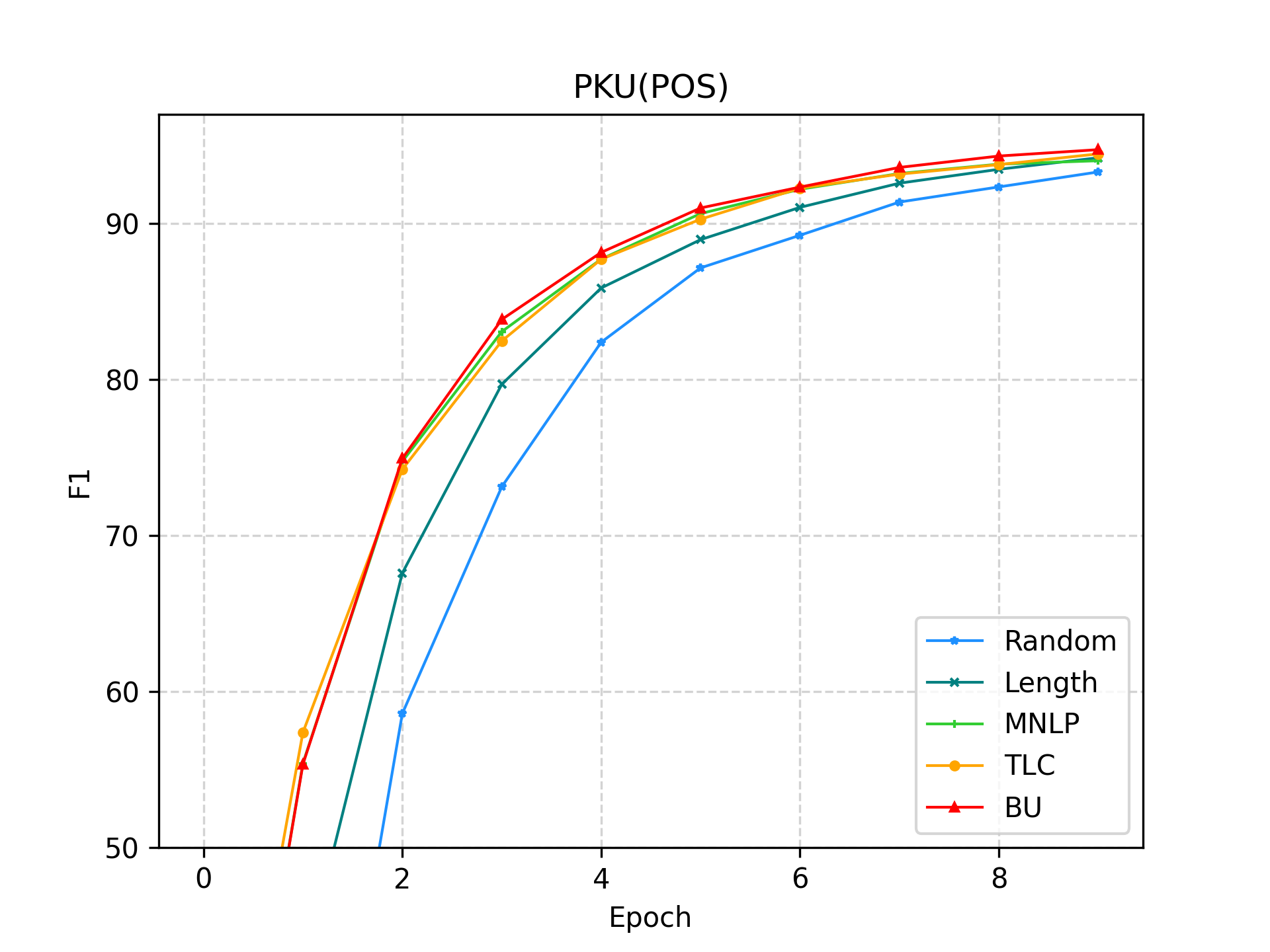
Figure 2: The F1 scores on the dev set of PKU with different difficulty metrics in the model-level CL training process.

In this section, we investigate the impact of various difficulty metrics during the model-level CL training process for the SynSemGCN model.

Figure 2 depicts the change in F1 scores on the PKU dataset development set over the initial 10 epochs of the model-level CL process. After 10 epochs, all training data are employed, so the initial 10 epochs offer insights into the influence of different metrics.

Observing the figure, we can discern that the four alternative difficulty metrics outperform the Random metric. Notably, a significant performance gap is evident between the Length metric and the three metrics introduced in this paper. BU, in particular, achieves the highest performance, suggesting that uncertainty-based metrics can select samples that align better with the model’s learning path, resulting in accelerated learning for the model.

4.5.   Effect of Hyper-parameters

$E_{grow}$		CTB5		PKU
	CWS	POS	CWS	POS
5	98.84	97.82	98.55	96.55
10	98.90	97.95	98.59	96.54
15	98.87	97.88	98.55	96.48

Table 7: The effect of $E_{grow}$ in Eq. 10.

$E_{0}$		CTB5		PKU
	CWS	POS	CWS	POS
5	98.90	97.95	98.59	96.54
10	98.88	97.82	98.54	96.51
15	98.91	97.83	98.54	96.49

Table 8: The impact of the number of epochs of teacher model, $E_{0}$.

In this section, we explore the impact of the hyperparameters on the performance of CL. The adjustment of the parameters is based on the SynSemGCN+TCL(BU) model.

First, we investigate the impact of the hyper-parameter $\lambda_{0}$ on CL performance. We conduct the experiments on the CTB5 dataset, tuning the value of $\lambda_{0}$ in the model-level pacing function Eq. 10, and the experimental results are represented by a line graph as shown in Figure 3. As observed, the model achieves optimal performance when $\lambda_{0}=0.3$. However, when the value exceeds 0.4, the model’s performance gradually deteriorates.

Additionally, we examine the impact of $E_{grow}$ in Eq. 10, which controls the number of epochs for $\lambda$ to reach 1. As shown in Table 7, when $E_{grow}$ is set to 10, the model exhibits superior performance on both the CTB5 and PKU datasets. Therefore, we adopt $E_{grow}$ as 10 epochs in our experiments.

Next, we assess the impact of the training epochs $E_{0}$ of the teacher model, which initializes the difficulty ranking of the training data for the student model. We aim to investigate whether a more mature teacher model contributes to improved performance. For this purpose, we conduct experiments on both the CTB5 and PKU datasets, utilizing teacher models trained for 5, 10, and 15 epochs to rank the initial training data for the student models.

The experimental results, as shown in Table 8, reveal that a more mature teacher model does not necessarily lead to better performance. Instead, the student model achieves optimal results when the teacher model is trained for 5 epochs. One possible explanation for this finding is that a teacher model with fewer training epochs aligns better with the initial state of the student model, allowing for a more suitable estimation of sample difficulty.

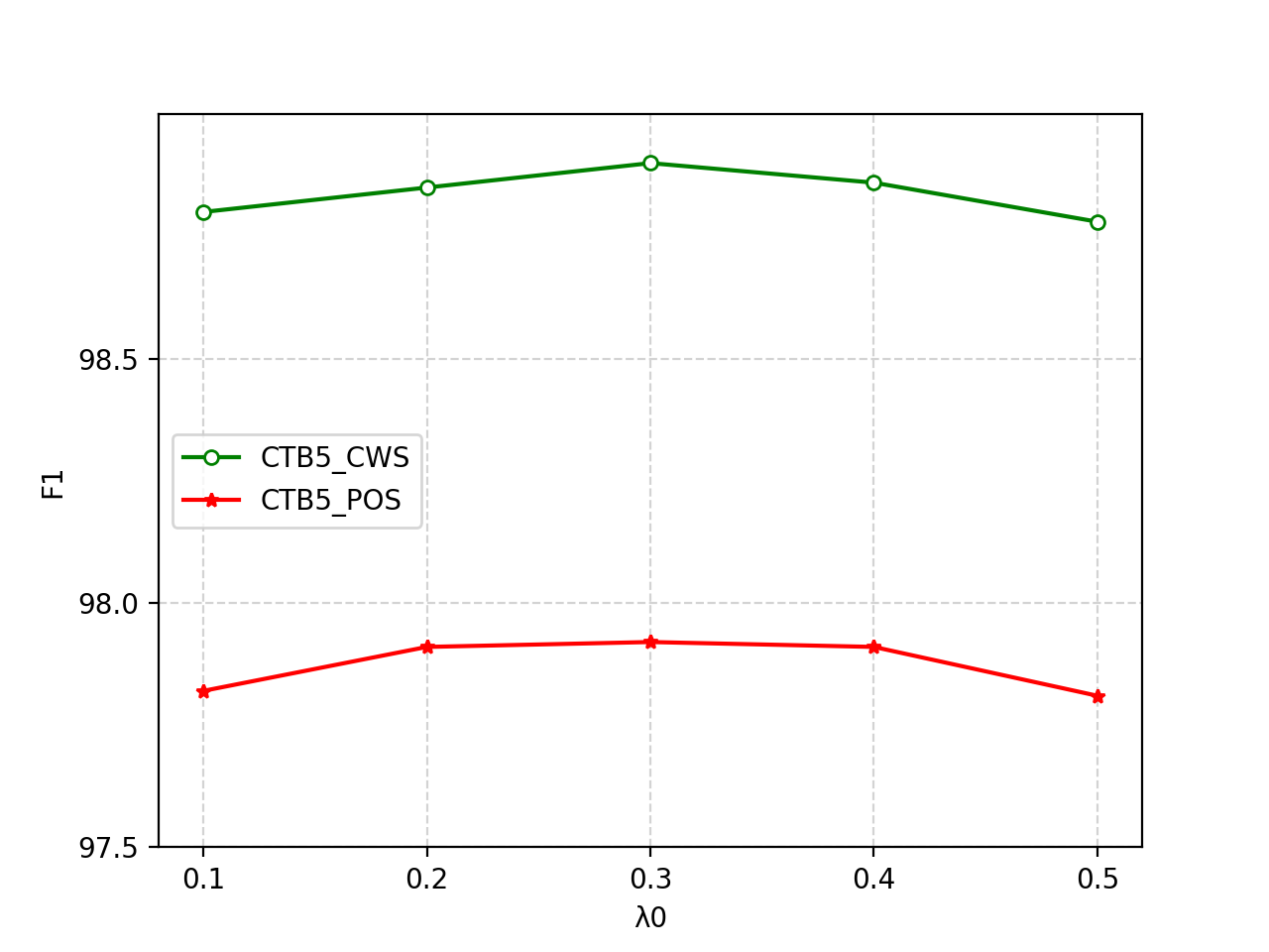
Figure 3: The impact of model-level curriculum learning hyper-parameters $\lambda_{0}$.

Finally, we explore the impact of different $K$ values on the BU difficulty metric, which determines the number of dropout times. The experiments are conducted on the CTB6 dataset, and the results are summarized in Table 9. Notably, the model achieves optimal performance when $K=3$. Therefore, we select $K=3$ for all the above experiments.

Due to space constraints, we do not report the experimental results for the variation of $N$ in the TLC metric. However, we can state that the best performance was experimentally demonstrated when $N=5$. In the future, we will add these experimental results in the appendix.

Para.		CTB6		PKU
	CWS	POS	CWS	POS
$K$=2	98.01	95.11	98.55	96.53
$K$=3	98.05	95.14	98.59	96.54
$K$=4	98.03	95.13	98.52	96.46

Table 9: The effect of of $K$ times dropout in BU difficulty metric.

5.   Conclusion

This paper introduces a novel two-stage curriculum learning framework aimed at enhancing performance and accelerating the training process for sequence labeling tasks. Focusing on the sequence labeling task of CWS and POS tagging, this framework demonstrates its effectiveness in improving results. To further broaden the scope of this framework, future research could explore its application to other sequence labeling tasks, such as named entity recognition

There are some limitations. First, our approach may not yield significant improvement when applied to small datasets. Additionally, the design of our difficulty metrics involves the setting of many hyperparameters, which may pose a challenge in terms of optimization.

6.   Bibliographical References