Abstract.

Online decision-makers today can often obtain predictions on future variables, such as arrivals, demands, inventories, and so on. These predictions can be generated from simple forecasting algorithms for univariate time-series, all the way to state-of-the-art machine learning models that leverage multiple time-series and additional feature information. However, the prediction quality is often unknown to decisions-makers a priori, hence blindly following the predictions can be harmful. In this paper, we address this problem by giving algorithms that take predictions as inputs and perform robustly against the unknown prediction quality.

We consider the online resource allocation problem, one of the most generic models in revenue management and online decision-making. In this problem, a decision maker has a limited amount of resources, and requests arrive sequentially. For each request, the decision-maker needs to decide on an action, which generates a certain amount of rewards and consumes a certain amount of resources, without knowing the future requests. The decision-maker’s objective is to maximize the total rewards subject to resource constraints. We take the shadow price of each resource as prediction, which can be obtained by predictions on future requests. Prediction quality is naturally defined to be the $\ell_{1}$ distance between the prediction and the actual shadow price. Our main contribution is an algorithm which takes the prediction of unknown quality as an input, and achieves asymptotically optimal performance under both requests arrival models (stochastic and adversarial) without knowing the prediction quality and the requests arrival model beforehand. We show our algorithm’s performance matches the best achievable performance of any algorithm had the arrival models and the accuracy of the predictions been known. Finally, we empirically validate our algorithm with experiments.

Key words: online resource allocation; decision-making with predictions; regret analysis; competitive analysis

1. Introduction

Allocating a limited number of resources to satisfy different requests as they arrive is a key ingredient to many operations problems. For example, companies in the airline industry need to decide on whether or not to accept a certain offer for a seat at a given price, while the total number of seats are limited (Talluri & Van Ryzin (2006); Ball & Queyranne (2009)); in online shopping, companies can choose a limited number of products to display to when a customer browses (McFadden et al. (1973); Gallego et al. (2004); Luce (2012)); internet search engine companies run a large auction at each time a consumer typing in keywords, where businesses place bids for their advertisements (Edelman et al. (2007); Mehta et al. (2007); Varian (2007)). Because resources are limited, making good decisions can be challenging. The Online Resource Allocation Problem is a generic model that covers these problems. In the Online Resource Allocation Problem, at each time period a request arrives, and the decision-maker needs to decide on an action to respond in an online fashion, i.e. without knowing future requests. Each action generates some reward and consumes some resources. The total number of resources are limited, and the objective is to maximize the total reward across all time periods subject to the resource constraint. While the Online Resource Allocation Problem is arguably ubiquitous in practice today, it may be worth highlighting a few motivating examples:

• Assortment: Consider an online marketplace. When a customer search for products on the site, the company needs to decide on a subset of products to display on each pages based on the customer’s preferences. The customer then chooses each product with a certain probability based on different assortments shown. In this assortment problem, the requests are customers’ searches, the set of actions are the set of possible assortments that the company can display, the reward of an action is the expected profit earned by displaying a certain assortment, and the resources are the inventories of the products. Therefore this assortment problem can be modelled as the Online Resource Allocation Problem.

• Revenue Management: One of the most traditional examples of revenue management appears in airline industry, where requests of seats arrive one by one, each comes with a difference price. The company needs to decide on whether or not to accept a request as it arrives. The total number of seats is limited, which can naturally be viewed as resources in the Online Resource Allocation Problem.

• Online Matching (AdWords, Online Auctions): Online matching is itself a general model formulating various two-sided markets, such as AdWords, online auctions, and so on. In the context of the Online Resource Allocation Problem, the online nodes (impressions in AdWords) can be viewed as the arrivals, and the capacities of the offline nodes (budgets of bidders) can be viewed as resources. Hence this class of problems is also a particular instance of the Online Resource Allocation Problem.

At present, there are by and large two existing approaches to the Online Resource Allocation Problem. The traditional approach to this problem is to assume an arrival model and develop algorithms that have worst-case guarantees. The two most popular arrival models are stochastic and adversarial, where the former assumes each arrival is drawn independently from an unknown underlying distribution, and the later assumes nothing on the future arrivals – they can be as bad as possible. Under the stochastic arrival model the performance of an algorithm is measured by its regret, and under the adversarial arrival model the performance of an algorithm is measured by its competitive ratio. Balseiro et al. (2023) gave an algorithm for the Online Resource Allocation Problem that achieves the optimal performance under both arrival models without knowing the actual arrival model, which solved the problem in the worst-case. However, the worst-case algorithms might be too pessimistic, since in reality the decision-maker often does have some insights on the future arrivals based on data/forecasts. This extra information can help us go beyond the worst-case analysis, which motivates another approach to the problem.

With developments in data acquisition and machine learning forecasts, the modern approach is to utilize some sort of predictions of information on the future arrivals. These predictions can be generic (i.e. with no statistical assumptions), ranging from simple time-series models to state-of-the-art machine learning algorithms. The de facto approach in practice is to then take these predictions as facts, that is, the decision-maker solves the problem offline using these predictions as true arrivals and take actions accordingly. However, because the decision-maker does optimization based on predictions, if predictions are inaccurate, their actions’ performances are bad. Moreover, it is possible to have inaccurate predictions due to factors such as insufficient amount of data, bad machine-learning model, and so on. Therefore, blindly following predictions also has its drawbacks.

To summarize so far, the Online Resource Allocation Problem admits algorithms with optimal worst-case guarantees, which can be made significantly better or worse by following predictions depending on the prediction quality. This suggests the opportunity to design an algorithm that leverages predictions optimally, in the sense that the predictions are utilized when accurate, and ignored when inaccurate. Ideally, such an algorithm should operate without knowledge of (a) the accuracy of the predictions and (b) the method with which they are generated. This is precisely what we accomplish in this paper.

1.1. The Online Resource Allocation with Predictions

The primary purpose of this paper is to develop an algorithm that optimally incorporates predictions (defined in the most generic sense possible) into the Online Resource Allocation Problem. Without predictions, the Online Resource Allocation Problem consists a finite horizon of $T$ time periods and a limited number of $m$ types of resources. At each time period, a decision must be made which will consume a certain set of resources and yield a certain reward. The form of these individual decision problems changes over time and is unknown in advance.

We consider two different arrival models: stochastic and adversarial. The stochastic arrival model assumes the arrivals are drawn independently from an unknown underlying distribution. Under the stochastic arrival model, we measure the performance of any algorithm using regret, which is the expected difference in the total reward earned by an optimal algorithm that “knows” the entire arrival sequence beforehand versus the reward earned by the algorithm. At minimum we aim to design algorithms that achieves sub-linear (i.e. $o(T)$) regret, as such an algorithm would earn a per-period reward that is on average no worse than the optimal, as $T$ grows. Under the adversarial arrival model, sub-linear regret is impossible to achieve in the worst case, so instead we measure the performance of any algorithm using competitive ratio, which is the ratio between the total reward earned by an optimal algorithm that “knows” the entire arrival sequence beforehand and the reward earned by the algorithm. In other words, if an algorithm is $\alpha$-competitive, then it can always obtain a total reward that is no less than $\frac{1}{\alpha}$ times the reward of the optimal algorithm. Arlotto & Gurvich (2019) proved that, without predictions, under the stochastic arrival model any algorithm incurs at least $\Omega(\sqrt{T})$ regret, and Balseiro & Gur (2019) proved that, without predictions, under the adversarial arrival model any algorithm has at least an $\alpha^{*}$ competitive ratio where $\alpha^{*}$ depends on the problem parameters. We seek to design algorithms that go beyond these worst-case bounds using predictions.

To this base problem, we introduce the notion of predictions. Our prediction is of the form of an $m$-dimensional vector $\hat{\mu}$ whose coordinates represent a predicted shadow price of each of the $m$ resources. We will show that this form of prediction satisfies certain nice properties including that it (a) immediately translates to a decision policy, and (b) there always exists “perfect” predictions which achieve near-optimal reward.

We naturally measure the quality of any prediction $\hat{\mu}$ by its $\ell_{1}$ distance from the closest perfect prediction $\mu^{*}$. Specifically, we use an accuracy parameter $a\in[0,\infty]$, defined as the largest $a$ such that $||\hat{\mu}-\mu^{*}||_{1}\in O(T^{-a})$. Notice that when $a=0$ the prediction is effectively useless, and as $a$ increases the prediction becomes more and more accurate. The intuition behind the dependence of $a$ on $T$ is the following: for the same prediction, the prediction is often more accurate if we are using it for the near future, say a week, as oppose to use it for a longer period of time, say a year. Therefore, for the same prediction $\hat{\mu}$, the accuracy parameter $a$ decreases as the time horizon $T$ increases. We call this problem the Online Resource Allocation with Predictions. Our primary challenge will be to design algorithms with performances that are robust in the prediction quality without having access to $a$.

1.2. Our Contributions

Our primary contributions can be summarized as follows.

1. Optimal Algorithms: We construct an algorithm that optimally leverages predictions, i.e. it is robust to unknown prediction accuracy. Suppose we are given a prediction $\hat{\mu}$ with accuracy parameter $a\in[0,\infty]$, i.e. $||\hat{\mu}-\mu^{*}||_{1}\in O(T^{-a})$. We give a single algorithm that achieves the optimal performance using predictions, without knowing the underlying arrival model (stochastic or adversarial) and without knowing the prediction accuracy.

Theorem 1.1 (Informal).

Without knowing the underlying arrival model (stochastic or adversarial) and without knowing $a$, given any constant $0<\delta<1$, there exists an algorithm which, with some mild (and tight) assumptions, achieves regret $\tilde{O}(T^{\frac{1}{2}-a})$ under the stochastic arrival model, and achieves reward $\max\{\frac{1}{\alpha^{*}}\textup{OPT},\textup{PRD}\}-\delta T$ under the adversarial arrival model.

Here $\alpha^{*}$ is the best competitive ratio which depends on the problem parameters that we will specify later, and OPT represents the optimal reward of a clairvoyant’s algorithm that knows the entire arrival sequence at the beginning. In other words, the highest achievable reward by any algorithm is $\frac{1}{\alpha^{*}}\text{OPT}$ under adversarial arrivals without predictions (Balseiro & Gur (2019)). On the other hand, simply following the actions induced by the prediction at each time also yields a certain amount of reward, which we denote by PRD. As we pointed out (and we will prove this later formally), for good predictions, PRD can be higher than $\frac{1}{\alpha^{*}}\text{OPT}$, and in fact it can be as high as OPT.

Our theoretical results are summarized in bold in Table 1, with a comparison to the problem with no predictions and the problem with prediction of known accuracy. Under the stochastic arrival model the performances listed are regrets, and under the adversarial arrival model the performances listed are rewards.

Arrival Model	Without	With Predictions of	With Predictions of
	Predictions	Known Accuracy	Unknown Accuracy
Stochastic (regret)	$O(T^{\frac{1}{2}})$	$O(T^{\frac{1}{2}-a})$	$\bm{\tilde{O}(T^{\frac{1}{2}-a})}$
Adversarial (reward)	$\frac{1}{\alpha^{*}}\text{OPT}$	$\max\{\frac{1}{\alpha^{*}}\text{OPT},\text{PRD}\}$	$\bm{\max\{\frac{1}{\alpha^{*}}\textbf{OPT},\textbf{PRD}\}-\delta T}$

Table 1. Summary of our main theoretical results (in bold). Each entry has a corresponding algorithm that, without knowing the underlying arrival model, achieves the stated performance simultaneously for both stochastic arrivals and adversarial arrivals. Each entry also has a matching lower bound.

2. Empirical Results: Finally, we demonstrate the practical value of our model (namely the Online Resource Allocation with Predictions) and our algorithm via empirical results on an H&M (Hennes & Mauritz AB) dataset, which contains two-year online sales data of 105,542 products. The experiment we conducted corresponds to the assortment problem we motivated above: when each customer checks out, we need to decide on three products to recommend based on the customer and the items in the shopping cart. The resources are the inventories of the products and the reward is the expected profit earned by our recommendation. At the beginning of each experiment, we are given a prediction on the shadow price of each product. The given predictions have varying qualities, which we generated using three different popular forecasting and machine learning algorithms. For each experiment, which runs for three months, we applied our algorithm and compared its performance against the two most-natural baseline algorithms: the optimal algorithm without predictions, and the simple policy which always utilizes the prediction (these correspond to the two “existing approaches” described previously). On any given experimental instance (i.e. a time-series and a prediction), the maximum (minimum) of the rewards gained by these two baselines can be viewed as the best (worst) we can hope for. Thus we measure performance in terms of the proportion of the gap between these two rewards gained by our algorithm, so if this “optimality gap” is close to 1, our algorithm performs almost as good as the better one of the two baselines.

We use three forecasting algorithms to generate predictions of various quality. We find that with Prophet forecasts, the average optimality gap is 0.68; with ARIMA forecasts, the average optimality gap is 0.58; with Exponential Smoothing forecasts, the average optimality gap is 0.53. This demonstrates that our algorithm performs well, irrespective of the quality of the predictions.

The remainder of this paper is organized as follows. The current section concludes with a literature review. In Section 2 we introduce our model of the Online Resource Allocation with Predictions. In Section 3 we present preliminary results of the problem without predictions as well as our main results. We then introduce our algorithms and proofs of main results in Section 4, which solves the Online Resource Allocation with Predictions under both arrival models without knowing the underlying arrival model. Section 5 contains our experimental results, and Section 6 concludes the paper.

1.3. Literature Review

Online Resource Allocation. Allocating scarce resources to satisfy requests arriving online has been extensively studied under various models. Related works assuming the arrivals are stochastic (i.i.d. or random order) including Devanur & Hayes (2009); Feldman et al. (2010); Devanur et al. (2011); Agrawal et al. (2014); Kesselheim et al. (2014) and Gupta & Molinaro (2016) where the objective is generally to achieve sub-linear worst-case regret. Another popular arrival model is the adversarial arrival model, under which is usually impossible to achieve sub-linear worst-case regret. Instead, the objective is to obtain a certain factor of the rewards of the offline optimum, which is called competitive analsis. For example, Mehta et al. (2007) and Buchbinder et al. (2007) studied the AdWords problem where they obtained a $(1-1/e)$-fraction of the optimal allocation in hindsight.

Apart from considering different arrival models separately, there has been a recent line of work in developing algorithms that achieve good performance under various arrival models simultaneously without knowing the underlying arrival model. Mirrokni et al. (2012) considered the AdWords problem and gave an algorithm with the optimal competitive ratio under adversarial arrivals and improved competitive ratios (though not asymptotic optimality) under stochastic arrivals. Balseiro et al. (2023) studied the Online Resource Allocation Problem and provided a mirror descent algorithm that achieves the optimal worst-case regret under stochastic arrivals and the optimal competitive ratio under adversarial arrivals. The main algorithm in our paper also attains the optimal performance under both stochastic and adversarial arrivals. Different from above, we first consider the two arrival models separately, and then perform a sequence of hypothesis tests to update the arrival model that our algorithm is based on. A popular approach for solving resource allocation problems is to design primal- and/or dual-based algorithms, and the algorithms in our paper also follow this regime.

Algorithms with Predictions. With the ubiquity of large data-sets and machine-learning models, theory and practice of augmenting online algorithms with machine-learned predictions have been emerging. This framework has lead to new models of algorithm analysis for going beyond worst-case analysis. Some applications on optimization problems including revenue optimization (Munoz & Vassilvitskii (2017); Balseiro et al. (2022); Golrezaei et al. (2023)), caching (Lykouris & Vassilvitskii (2021); Rohatgi (2020)), online matching (Lavastida et al. (2021); Jin & Ma (2022)), online scheduling (Purohit et al. (2018); Lattanzi et al. (2020)), the secretary problem (Antoniadis et al. (2020); Dütting et al. (2021, 2023)), and the nonstationary newsvendor problem (An et al. (2023)). Most of the related works analyzed the algorithms’ performances using competitive analysis and obtain optimal consistency-robustness (consistency-competitiveness) trade-off, where consistency is the competitive ratio of the algorithm when the prediction is accurate, and robustness (competitiveness) is the competitive ratio of the algorithm regardless the prediction’s accuracy. In contrary, under the stochastic arrivals we do regret analysis on our algorithm and prove our algorithm has near-optimal worst-case regret without knowing the prediction quality. Other papers that do regret analysis under the prediction model that we are aware of include Munoz & Vassilvitskii (2017) (revenue optimization in auctions), An et al. (2023) (nonstationary newsvendor), and Hu et al. (2024) (constrained online two-stage stochastic optimization). In general this approach is still largely new.

Finally, the closest works to our own are Balseiro et al. (2022) and Golrezaei et al. (2023), both of which are limited in the following two ways. First, the “base” problems they analyze (i.e. without predictions) are strict special cases of the Online Resource Allocation Problem we study. Second, they treat prediction quality as binary: predictions are either entirely accurate or entirely inaccurate. Under this assumption, they successfully designed algorithms that achieve the optimal consistency-robustness (consistency-competitiveness) tradeoff. On the other hand, as stated earlier, we will quantify prediction quality, and provide tight guarantees for predictions of any quality.

2. Model: The Online Resource Allocation with Predictions

In this section, we first formally define the Online Resource Allocation with Predictions problem, and then describe two standard arrival models (stochastic and adversarial) as well as their respective performance metrics.

2.1. Problem Formulation

Online Resource Allocation: Consider a problem over $T$ time periods labeled $t=1,\dots,T$. Assume there are $m$ different types of resources. The total number of resources available is denoted by $\rho T$, where $\rho\in\mathbb{R}^{m}_{+}$ is a non-negative $m$-dimensional vector. At each time period $t$, the decision-maker receives an arrival $\gamma_{t}=(r_{t},g_{t},\mathcal{X}_{t})\in\mathcal{S}$. Here, $r_{t}:\mathcal{X}_{t}\to\mathbb{R}_{+}$ is a non-negative reward function, $g_{t}:\mathcal{X}_{t}\to\mathbb{R}^{m}_{+}$ is a non-negative resource consumption function, $\mathcal{X}_{t}\subset\mathbb{R}^{d}_{+}$ is a compact action space, and $\mathcal{S}$ denotes the set of all possible arrivals. Note that we impose no convexity assumptions: $r_{t}(\cdot)$ can be non-concave, $g_{t}(\cdot)$ can be non-convex, and $\mathcal{X}_{t}$ can be non-convex or discrete. At each arrival $\gamma_{t}$, without knowing any of the future arrivals, an action $x_{t}\in\mathcal{X}_{t}$ must be selected, which yields $r_{t}(x_{t})$ reward and consumes $g_{t}(x_{t})$ resources. The objective is to maximize the total reward subject to the resource constraint. Finally, we assume that $\mathcal{X}_{t}$ always contains a $0$ vector representing a “void” action that consumes no resources and yields no rewards: $r(0)=0$ and $g_{t}(0)=0$. This ensures that there is always a feasible action available. This is the problem we will refer to as Online Resource Allocation (without predictions).

It will be convenient here to introduce some notation that will appear in our results later on (though our algorithms will not depend on these parameters). We denote by $\underline{\rho}=\min_{j\in[m]}\rho_{j}>0$ the lowest resource parameter and $\bar{\rho}=\max_{j\in[m]}\rho_{j}=||\rho||_{\infty}$ the highest resource parameter. Similarly, let $\bar{r}\geq 0$ be a constant which satisfies $\max_{x\in\mathcal{X}}r(x)\leq\bar{r}$ for every $(r,g,\mathcal{X})\in S$, and let $\bar{g}\geq\underline{g}>0$ be constants satisfying $\underline{g}\leq||g(x)||_{\infty}\leq\bar{g}$ for every $x\in\mathcal{X}$ and $x\neq 0$.

Primal and Dual: For any series of arrivals $\vec{\gamma}=(\gamma_{1},\dots,\gamma_{T})$, we use $\text{OPT}(\vec{\gamma})$ to denote the offline/hindsight optimum, which is the reward of the optimal solution when $\vec{\gamma}$ is known in advance:

(2.1) $$\text{OPT}(\vec{\gamma}):=\max_{x_{t}\in\mathcal{X}_{t}}\sum_{t=1}^{T}r_{t}(x_{t})\quad\text{ s.t. }\quad\sum_{t=1}^{T}g_{t}(x_{t})\leq\rho T.$$

As we will describe momentarily, it will be natural to consider predictions in terms of the dual space, so the Lagrangian dual problem of Eq. 2.1 plays a key role. Let $\mu\in\mathbb{R}^{m}_{+}$ be the vector of dual variables, where each $\mu_{j}$ can be thought of as the shadow price of resource $j$. We define

(2.2) $$r^{*}_{t}(\mu):=\sup_{x\in\mathcal{X}_{t}}\{r_{t}(x)-\mu^{\top}g_{t}(x)\}$$

as the optimal opportunity-cost-adjusted reward of request $\gamma_{t}$, where the opportunity cost is calculated according to the shadow prices $\mu$. Note that $r_{t}^{*}(\mu)$ is a generalization of the convex conjugate of $r_{t}(x)$ that takes the resource consumption function $g_{t}(x)$ and the action space $\mathcal{X}_{t}$ into account. In particular, when $g_{t}(x)=x$ and $\mathcal{X}_{t}$ is the whole space, $r_{t}^{*}(\mu)$ becomes the standard convex conjugate. For fixed arrivals $\vec{\gamma}$, we define the Lagrangian dual function $D(\mu\mid\vec{\gamma}):\mathbb{R}_{m}^{+}\to\mathbb{R}$ to be

(2.3) $$D(\mu\mid\vec{\gamma}):=\sum_{t=1}^{T}r_{t}^{*}(\mu)+\mu^{\top}\rho T.$$

This allows us to move the constraints of Eq. 2.1 to the objective, which is easier to work with. We equip the primal space of the resource constraints $\mathbb{R}^{m}$ with the $\ell_{\infty}$ norm $||\cdot||_{\infty}$, and the Lagrangian dual space with the $\ell_{1}$ norm $||\cdot||_{1}$. Such choices of norms come naturally from our analysis. Similar performance guarantees of our algorithms with the dependence on the number of resources can be obtained using the $\ell_{p}$ norm for the primal space and the $\ell_{q}$ norm for the primal space with $1/p+1/q=1$ and $p\in[2,\infty]$.

We will assume that the primal optimization problems in Eq. 2.2 admit an optimal solution. This is to simplify the exposition – our results still holds if we have an approximate of the optimal solution (see Balseiro et al. (2023)). By Weierstrass’ theorem, a sufficient condition for the existence of optimal solutions is that the reward function $r(\cdot)$ is upper-semicontinuous, the resource consumption function $g(\cdot)$ is component-wise lower-semicontinuous, and the action set $\mathcal{X}$ is compact.

Predictions: So far, we have presented the problem of Online Resource Allocation without predictions. As described in the introduction, it is often the case that when this problem is faced in practice, some notion of a “prediction” can be made which might guide us in selecting actions. Such predictions can come from a diverse set of sources ranging from simple human judgement, to forecasting algorithms built on previous demand data, to more-sophisticated machine learning algorithms trained on feature information. The process of sourcing or constructing such predictions is orthogonal to our work. Instead, we treat these predictions as given to us endogenously (and in particular, we make no assumption on the accuracy of these predictions), and attempt to use these predictions optimally.

Notice that from Eq. 2.2, at each time $t$, given a dual variable $\mu\in\mathbb{R}_{+}^{m}$ there is a natural action to take, namely the action

$$x^{\mu}_{t}\in\operatorname*{arg\,max}_{x\in\mathcal{X}_{t},\sum_{s=1}^{t-1}g_{s}(x_{s})+g_{t}(x)\leq\rho T}\left\{r_{t}(x)-\mu^{\top}g_{t}(x)\right\}.$$

In words, $x^{\mu}_{t}$ is the “greedy” action that, subject to the resource constraint, maximizes the opportunity-cost-adjusted reward according to the shadow prices $\mu$. Therefore, dual variables induces action, which makes them a natural quantity to predict. We will use the phrase “following $\mu$” to represent an algorithm which takes the actions induced by $\mu$ at every time period. We say a dual variable $\mu^{*}$ is a “perfect” dual variable if following $\mu^{*}$ yields rewards that is at most a constant away from OPT (which is essentially optimal). It can be shown that there always exists a “perfect” dual variable to follow:

Proposition 2.1 (“Perfect” Dual Variable).

Let $\mu^{*}\in\operatorname*{arg\,max}_{\mu\in\mathbb{R}^{m}_{+}}\sum_{t=1}^{T}r_{t}(x^{\mu}_{t})$ where $x^{\mu}_{t}\in\operatorname*{arg\,max}_{x\in\mathcal{X}_{t},\sum_{s=1}^{t-1}g_{s}(x_{s})+g_{t}(x)\leq\rho T}\left\{r_{t}(x)-{\mu}^{\top}g_{t}(x)\right\}$ are the actions induced by $\mu$. Then

$$\sum_{t=1}^{T}r_{t}(x^{\mu^{*}}_{t})+(\bar{g}/\underline{g}+1)(m+1)\bar{r}\geq\textup{OPT}(\vec{\gamma}).$$

The proof of Proposition 2.1 appears in Appendix A, and utilizes the Shapley-Folkman Theorem. In words, Proposition 2.1 shows that there exists a dual variable $\mu^{*}$ that is essentially optimal to follow. Note that there may exist multiple perfect dual variables.

With the understanding of the key role that dual variables play in our problem, we are ready to formally introduce the notion of predictions. We assume that before the first time period, the decision-maker receives a prediction $\hat{\mu}\in\mathbb{R}^{m}_{+}$ of the dual variable $\mu$. We measure the prediction error of $\hat{\mu}$ by $||\hat{\mu}-\mu^{*}||_{1}$, its $\ell_{1}$ distance from $\mu^{*}$. In the case that multiple perfect dual variables exist, we take $\mu^{*}$ to be the perfect dual variable that is closest to $\hat{\mu}$. We quantify the prediction error using the accuracy parameter, which is the smallest $a\in[0,\infty]$ such that

(2.4) $$||\hat{\mu}-\mu^{*}||_{1}\leq\kappa T^{-a}.$$

Here $\kappa>0$ is a scaling constant that we can choose (later in this section we will see a natural choice of $\kappa$, but any $\kappa$ that ensures $a\in[0,\infty]$ can be chosen, and it will not change our performance bound asymptotically). The two extreme cases of the prediction error are (1) $a=0$, in which case $\hat{\mu}$ is almost a constant away from $\mu^{*}$, so the prediction is effectively useless; and (2) $a=\infty$, in which case $\hat{\mu}=\mu^{*}$, so the prediction is perfect. We will always assume that $a$ is unknown to the decision-maker.

In reality, a prediction $\hat{\mu}$ is unlikely to be completely useless. We make the following technical assumption on the prediction quality:

Assumption 2.1 (Non-trivial Prediction).

There exists a (known) function $\epsilon(T)=o(1)$ such that $||\hat{\mu}-\mu^{*}||_{1}=o(\epsilon(T))$.

Note that 2.1 does not eliminate the case $a=0$. In practice $\epsilon(T)$ can be chosen to be a function close to 1 without hurting the algorithm’s performance guarantee.

2.2. Arrival Models and Performance Metrics

An online algorithm ALG, at each time period $t$, takes an action $x_{t}$ (potentially randomized, but deterministic here to save on notation) based on the prediction $\hat{\mu}$, the current request $\left(r_{t},g_{t},\mathcal{X}_{t}\right)$ and the previous history $\mathcal{H}_{t-1}:=\left\{r_{s},g_{s},\mathcal{X}_{s},x_{s}\right\}_{s=1}^{t-1}$, i.e., $x_{t}=\text{ALG}\left(r_{t},g_{t},\mathcal{X}_{t}\mid\hat{\mu},\mathcal{H}_{t-1}\right)$. We denote the reward received by an algorithm on an arrival sequence $\vec{\gamma}$ as

$$R(\text{ALG}\mid\vec{\gamma})=\sum_{t=1}^{T}r_{t}\left(x_{t}\right).$$

Note that when defining the notion of predictions, we essentially introduced one algorithm, which is simply to follow the prediction $\hat{\mu}$. Here we formally define this algorithm, which we call the Prediction Algorithm (PRD):

Inputs: Prediction $\hat{\mu}$, total time periods $T$, initial resources $G_{1}=\rho T$;

for $t=1,\ldots,T$  do

       Receive request $\left(r_{t},g_{t},\mathcal{X}_{t}\right)$;

       Make the primal decision $x_{t}$ and update the remaining resources $G_{t}$:

       $x_{t}\in\arg\max_{x\in\mathcal{X}_{t},g_{t}(x)\leq G_{t}}\left\{r_{t}(x)-\hat{\mu}^{\top}g_{t}(x)\right\}$;
$G_{t+1}\leftarrow G_{t}-g_{t}\left(x_{t}\right).$

Algorithm 1 Prediction Algorithm (PRD)

As stated in Proposition 2.1, if $a=\infty$, i.e., if $\hat{\mu}=\mu^{*}$, then $R(\text{PRD}\mid\vec{\gamma})+(\bar{g}/\underline{g}+1)(m+1)\overline{r}\geq\textup{OPT}(\vec{\gamma})$, which shows the Prediction Algorithm is essentially optimal if we have a perfect prediction.

Note that for any sequence of dual variables $\mu_{1},\dots,\mu_{T}$, following $\mu_{t}$ at time period $t$ gives a series of actions $x_{1},\dots,x_{t}$. We define the depletion time of resource $j$ by following $\mu_{1},\dots,\mu_{T}$ to be the first time period such that the remaining amount of resources $j$ is less than $\underline{g}$, that is, after this time period no actions that consumes resource $j$ is feasible (if this never happens we set the depletion time to be $T$). We will use the depletion time to quantify the behavior of $\hat{\mu}$. Intuitively, dual variables close to $\hat{\mu}$ induce similar actions in most time periods as long as $\hat{\mu}$ is not always on the “boundary” of decisions, and hence their depletion time should be similar. We make this idea formal using the following assumption on the depletion time.

Assumption 2.2 (Non-degenerate Prediction).

There exists a constant $\zeta>0$ that satisfies the following: for any sequence of dual variables $\mu_{1},\dots,\mu_{T}$ where $\mu_{t}\in\mathbb{R}^{m}_{+}$ and $||\hat{\mu}-\mu_{t}||_{1}\leq\zeta$ for all $t$, the difference between the depletion time of resource $j$ by following $\mu_{1},\dots,\mu_{T}$ and by following $\hat{\mu}$ is in $o(T)$ for every resource $j$.

2.2 roughly states that, for a sequence of dual variables that is close to the prediction, the action induced by the sequence of dual variables and the action induced by the prediction deplete resources at similar times. This assumption is reasonable and mild for the following reasons: in reality, most actions sets are discrete (such as $\{\text{accept,reject}\}$, $\mathbb{N}$, etc.). Therefore for most $\hat{\mu}$, as long as it is not at the “boundary” (which is often a measure-zero set), dual variables close to $\hat{\mu}$ all induce the same action. Moreover, in practice it is also unlikely for the “boundaries” at each time period to be the same across a majority of time periods since $r_{t}(\cdot)$ and $g_{t}(\cdot)$ vary over time, in which case 2.2 is satisfied with any prediction $\hat{\mu}$. Finally, perturbing each input with some small noise also turns a degenerate prediction into a non-degenerate one.

There are two primary arrival models when studying online problems: the stochastic (i.i.d) arrival model and the adversarial arrival model, both which we define formally below. Our goal is to design algorithms that have good performances under both arrival models, and for predictions of different qualities. Additionally, our algorithms should be oblivious to the arrival model and the prediction quality, i.e., they should have good performance without knowing the arrival model and the prediction quality.

Stochastic (i.i.d.) Arrival Model: The arrivals are drawn independently from an (unknown) underlying probability distribution $\mathcal{P}\in\Delta(\mathcal{S})$, where $\Delta(\mathcal{S})$ is the space of all probability distributions over $\mathcal{S}$. We measure the performance of an algorithm by its regret. Given an underlying arrival distribution $\mathcal{P}$, the regret incurred by an algorithm ALG under $\mathcal{P}$ is defined as $\mathbb{E}_{\vec{\gamma}\sim\mathcal{P}^{T}}[\text{OPT}(\vec{\gamma})-R(\text{ALG}\mid\vec{\gamma})]$. We will be concerned with the worst-case regret over all distributions in $\Delta(\mathcal{S})$: we define the regret of ALG to be

$$\text{Regret}(\text{ALG})=\sup_{\mathcal{P}\in\Delta(\mathcal{S})}\mathbb{E}_{\vec{\gamma}\sim\mathcal{P}^{T}}[\text{OPT}(\vec{\gamma})-R(\text{ALG}\mid\vec{\gamma})].$$

Note that if the regret $\text{Regret}(\text{ALG})$ is sub-linear in $T$, then algorithm ALG is essentially optimal on average as $T$ goes to infinity.

Adversarial Arrival Model: The arrivals are arbitrary and chosen adversarially. Unlike the stochastic arrival model, regret here can be shown to grow linearly with $T$ for any algorithm, so it is less meaningful to study the order of regret over $T$. Instead, we use competitive ratio as the performance metric. We say that an algorithm ALG is asymptotically $\alpha$-competitive if $\alpha\geq 1$ is the smallest number such that

$$\limsup_{T\to\infty}\sup_{\vec{\gamma}\in\mathcal{S}^{T}}\left\{\frac{1}{T}\big{(}\text{OPT}(\vec{\gamma})-\alpha R(\text{ALG}\mid\vec{\gamma})\big{)}\right\}\leq 0.$$

In words, if an algorithm is asymptotically $\alpha$-competitive, then it can obtain at least $1/\alpha$ fraction of the optimal reward in hindsight as $T$ goes to infinity.

Now Balseiro & Gur (2019) proved that, without predictions, the lowest competitive ratio that any algorithm can achieve is $\alpha^{*}=\max\{\sup_{(r,g,\mathcal{X})\in\mathcal{S}}\sup_{j\in[m],x\in\mathcal{X}}g(x)_{j}/\rho_{j},1\}$. Balseiro et al. (2023) gave a mirror descent algorithm that achieves this competitive ratio, which we will introduce in the next subsection. This is, loosely speaking, the best we might hope to achieve with “bad” predictions. On the other hand, we can always obtain $R(\text{PRD}\mid\vec{\gamma})$ by following the prediction, which may exceed $\text{OPT}(\vec{\gamma})/\alpha^{*}$ with “good” predictions (indeed, as we have seen in Proposition 2.1, $R(\text{PRD}\mid\vec{\gamma})$ can be as large as $\text{OPT}(\vec{\gamma})$).

If we knew the prediction quality beforehand, we could obtain the maximum of the two by simply choosing the better approach (this is in fact the best we can hope for). Using this as the benchmark, we will compare an algorithm’s reward to this maximum. That is, for an algorithm ALG, we will analyze the following quantity:

$$\limsup_{T\to\infty}\sup_{\vec{\gamma}\in\mathcal{S}^{T}}\left\{\frac{1}{T}\left(\max\left\{\frac{1}{\alpha^{*}}\text{OPT}(\vec{\gamma}),R(\text{PRD}\mid\vec{\gamma})\right\}-R(\text{ALG}\mid\vec{\gamma})\right)\right\}.$$

3. Main Results

In this section, we first present previous results for the Online Resource Allocation problem without predictions, and then give our main results on the full problem (with predictions) along with matching lower bounds.

3.1. Prior Results: Online Resource Allocation without Predictions

Balseiro et al. (2023) studied no-prediction version of our problem,and gave a mirror descent algorithm which achieves the “best” achievable performance under both arrival models without knowing the underlying arrival model.

Inputs: Initial dual solution $\mu_{1}$, total time periods $T$, initial resources $G_{1}=\rho T$, reference function $h(\cdot):\mathbb{R}^{m}\rightarrow\mathbb{R}$, and step-size $\eta$;

for $t$ from $1$ to $T$ do

       Receive request $\left(r_{t},g_{t},\mathcal{X}_{t}\right)$;

       Make the primal decision $x_{t}$ and update the remaining resources $G_{t}$: $x_{t}\in\arg\max_{x\in\mathcal{X}_{t},g_{t}(x)\leq G_{t}}\left\{r_{t}(x)-\mu_{t}^{\top}g_{t}(x)\right\}$;
$G_{t+1}\leftarrow G_{t}-g_{t}\left(x_{t}\right).$

      Obtain a sub-gradient of the dual function: $\phi_{t}\leftarrow-g_{t}\left(x_{t}\right)+\rho.$

      Update the dual variable by mirror descent:

(3.1) $$\mu_{t+1}\leftarrow\arg\min_{\mu\in\mathbb{R}_{+}^{m}}\phi_{t}^{\top}\mu+\frac{1}{\eta}V_{h}\left(\mu,\mu_{t}\right),$$

where $V_{h}(x,y):=h(x)-h(y)-\nabla h(y)^{\top}(x-y)$ is the Bregman divergence.

Algorithm 2 Mirror Descent Algorithm (MDA)

The Mirror Descent Algorithm takes an initial dual variable, a step-size, and a reference function as inputs. At each time period $t$, the algorithm takes the action induced by the current dual variable $\mu_{t}$, and performs a first-order update on the dual variable. For the updating step, note we can write the dual function in Eq. 2.3 as $D(\mu\mid\vec{\gamma}):=\sum_{t=1}^{T}D_{t}(\mu\mid\vec{\gamma})$ where the $t$-th term of the dual function is given by $D_{t}(\mu\mid\vec{\gamma})=r_{t}^{*}(\mu)+\mu^{\top}\rho$. Then it follows that $\phi_{t}:=-g_{t}\left(x_{t}\right)+\rho$ is a sub-gradient of $D_{t}(\mu\mid\vec{\gamma})$ at $\mu_{t}$ under our assumptions by Danskin’s Theorem (see, e.g., Proposition B.25 in Bertsekas (1997)), and the algorithm uses $\phi_{t}$ to update the dual variable by performing a mirror descent step in Eq. 3.1 with step-size $\eta$ and reference function $h(\cdot)$. Intuitively, the Mirror Descent Algorithm tries to find dual variables via gradient information such that these dual variables induce actions with good primal performances. For more on mirror descent algorithms in general, see Nemirovskij & Yudin (1983); Beck & Teboulle (2003); Hazan et al. (2016); Lu et al. (2018).

For completeness, we state the standard assumptions on choosing the reference function $h(\cdot)$ for mirror descent algorithms (Beck & Teboulle (2003); Bubeck et al. (2015); Lu et al. (2018); Lu (2019)). These assumptions are applicable to all algorithms in our paper.

• $h(\mu)$ is either differentiable or essentially smooth (Bauschke et al. (2001)) and Lipschitz in $\mathbb{R}^{m}_{+}$;

• $h(\mu)$ is $\sigma$-strongly convex with respect to the $\ell_{1}$-norm in $\mathbb{R}^{m}_{+}$, i.e., $h(\mu_{1})\geq h(\mu_{2})+\nabla h(\mu_{2})^{\top}(\mu_{1}-\mu_{2})+\frac{\sigma}{2}||\mu_{1}-\mu_{2}||_{1}^{2}$ for all $\mu_{1},\mu_{2}\in\mathbb{R}^{m}_{+}$.

• $h(\mu)$ coordinately-wise separable, i.e., $h(\mu)=\sum_{j=1}^{m}h_{j}(\mu_{j})$ where $h_{j}:\mathbb{R}_{+}\to\mathbb{R}$ is an univariate function. Moreover, for every resource $j$ the function $h_{j}$ is $\sigma^{\prime}$-strongly convex with respect to the $\ell_{1}$-norm over $[0,\mu_{j}^{\max}]$ where $\mu_{j}^{\max}:=\bar{r}/\rho_{j}+1$.

Note that by Weierstrass’ Theorem our assumptions guarantee that the projection step in Eq. 3.1 always admits a solution.

Balseiro et al. (2023) proved the following performance guarantee for the Mirror Descent Algorithm:

Proposition 3.1 (Theorem 1 and Theorem 2 in Balseiro et al. (2023)).

Consider the Mirror Descent Algorithm (MDA) with step-size $\eta\sim T^{-1/2}$ and initial solution $\mu_{1}\in\mathbb{R}^{m}_{+}$. It holds that:

• If the arrivals are stochastic,

  $$\textup{Regret}(\textup{MDA})\leq C_{1}+(C_{2}+C_{3})\sqrt{T};$$

• If the arrivals are adversarial, for any adversarially chosen $\vec{\gamma}$,

  $$\textup{OPT}(\vec{\gamma})-\alpha^{*}R(\textup{MDA}\mid\vec{\gamma})\leq C_{1}+\alpha^{*}(C_{2}+C_{3})\sqrt{T};$$

where $C_{1}=\bar{r}\bar{g}/\underline{\rho}$, $C_{2}=(\bar{g}+\bar{\rho})^{2}/2\sigma$, $C_{3}=\max\{V_{h}(\mu,\mu_{1}):\mu\in\{0,(\bar{r}/\rho_{1})e_{1},\dots,(\bar{r}/\rho_{m})e_{m}\}\}$ and where $e_{j}\in\mathbb{R}^{m}$ is the $j$-th unit vector.

Proposition 3.1 shows that the Mirror Descent Algorithm achieves $O(\sqrt{T})$ regret and is $\alpha^{*}$-competitive, which are both optimal (Arlotto & Gurvich (2019); Balseiro & Gur (2019)).

Finally, as a technical aside, there is now a natural choice for the scaling constant $\kappa$ in defining the prediction error Eq. 2.4: Balseiro et al. (2023) showed that if the initial dual solution satisfies $\mu_{1}\leq\mu^{\max}$ where $\mu^{\max}_{j}=\bar{r}/\rho_{j}+1$, then $\mu_{t}\leq\mu^{\max}$ for any $t$. This implies that it is enough to only consider dual variables that lie in the $m$-dimensional rectangle $[0,\mu^{\max}_{1}]\times\cdots\times[0,\mu^{\max}_{m}]\in\mathbb{R}_{+}^{m}$. Therefore we may assume without loss of generality that the prediction $\hat{\mu}$ we receive lies inside this rectangle (otherwise we could project $\hat{\mu}$ onto this rectangle). Thus setting $\kappa=||\mu^{\max}||_{1}$ ensures $a\in[0,\infty]$.

3.2. Prior Results: Lower Bounds

As a final step before describing our results, we present previous lower bounds for the full problem with predictions and known arrival model.

Stochastic Arrivals: Without predictions, the best achievable regret by any algorithm is on the order of $O(\sqrt{T})$ (Arlotto & Gurvich (2019)). With predictions, Orabona (2013) gave the following lower bound on the best achievable regret with known accuracy parameter $a$:

Proposition 3.2 (Corollary of Theorem 2 in Orabona (2013)).

Under the stochastic arrival model, given a prediction $\hat{\mu}$ with accuracy parameter $a$, no algorithm can achieve regret better than $O(\max\{T^{\frac{1}{2}-a},1\})$, even if $a$ is known.

Adversarial Arrivals: Without predictions, the best achievable reward by any algorithm (taken the worst-case $\vec{\gamma}$ across all problem instances) is $\frac{1}{\alpha^{*}}\text{OPT}(\vec{\gamma})$ (Balseiro & Gur (2019)). On the other hand, simply following the actions induced by the prediction at each time yields reward $R(\text{PRD}\mid\vec{\gamma})$. As we have seen in Proposition 2.1, for good predictions $R(\text{PRD}\mid\vec{\gamma})$ can be higher than $\frac{1}{\alpha^{*}}\text{OPT}(\vec{\gamma})$, and in fact it can be as high as $\text{OPT}(\vec{\gamma})$. Therefore we have the following lower bound under adversarial arrivals:

Proposition 3.3 (Corollary of Theorem 3.1 in Balseiro & Gur (2019)).

Under the adversarial arrival model, given a prediction with accuracy parameter $a$, no algorithm can achieve (worst-case $\vec{\gamma}$ across all problem instances) reward higher than $\max\{\frac{1}{\alpha^{*}}\textup{OPT}(\vec{\gamma}),R(\textup{PRD}\mid\vec{\gamma})\}$, even if $a$ is known.

3.3. Our Results: Online Resource Allocation with Predictions

We are finally prepared to state our main result, which to develop a single algorithm that achieves the optimal performance using predictions, without knowing the underlying arrival model and the prediction accuracy.

Theorem 3.1.

Assume that Assumptions 2.1, 2.2, and 4.1 hold. Given a prediction $\hat{\mu}$ with (unknown) accuracy parameter $a$, and given any constant $0<\delta<1$, there exists an algorithm (MainALG) such that:

1. If the arrivals are stochastic,

   $$\textup{Regret}(\textup{MainALG})=\tilde{O}(\max\{T^{\frac{1}{2}-a},1\});$$

2. If the arrivals are adversarial,

   $$\limsup_{T\to\infty}\sup_{\vec{\gamma}\in\mathcal{S}^{T}}\left\{\frac{1}{T}\left(\max\left\{\frac{1}{\alpha^{*}}\textup{OPT}(\vec{\gamma}),R(\textup{PRD}\mid\vec{\gamma})\right\}-R(\textup{MainALG}\mid\vec{\gamma})-\bar{r}\delta T\right)\right\}\leq 0.$$

A few remarks are in order:

• Since our result applies for any constant $0<\delta<1$, as a corollary of the above two lower bounds, this result is also essentially tight. It can be made exactly tight if any non-trivial lower bound on OPT is known. In practice, $\delta$ can simply be taken to be $1/T$.

• Assumption 4.1, which will be stated in the next section, essentially requires that if the arrival model is adversarial, then the adversary may not be “deceptively stochastic” in a limited, but precise way. Specifically, an adversary could select an arrival sequence which initially appears to be stochastic (making this idea precise is non-trivial), in such a manner as to encourage an algorithm to deplete resources at an incorrect pace. Assumption 4.1 makes a small restriction on this behavior. It is critical to emphasize that some sort of assumption is necessary here, as the following lower bound demonstrates:

Proposition 3.4.

For any algorithm, there exists a sequence of instances $\vec{\gamma}_{T}$ of increasing time horizon $T$ that satisfies Assumptions 2.1 and 2.2, for which at least one of the following holds:

1. The arrival model is stochastic, and

   $$\textup{Regret}(\textup{ALG})=\Omega(T);$$

2. The arrival model is adversarial, and

   $$\limsup_{T\to\infty}\left\{\frac{1}{T}\left(\max\left\{\frac{1}{\alpha^{*}}\textup{OPT}(\vec{\gamma}_{T}),R(\textup{PRD}\mid\vec{\gamma}_{T})\right\}-R(\textup{ALG}\mid\vec{\gamma}_{T})\right)\right\}\geq\Omega(1).$$

Proof of Proposition 3.4..

Set $\rho=1$. Consider two different arrivals $\gamma^{1}=(r^{1},g^{1},\mathcal{X})$ and $\gamma^{2}=(r^{2},g^{2},\mathcal{X})$, where $\mathcal{X}=\{0,1\}$ (one can think of this as {reject, accept}). Set $r^{1}(1)=1,g^{1}(1)=1,r^{2}(1)=\bar{r}$, $g^{2}(1)=\alpha^{*}$, and $\bar{r}/\alpha^{*}>1+1/\log(T)$ . Let $\hat{\mu}=1+1/\log(T)$ be the prediction, then following $\hat{\mu}$ means taking action 0 for $\gamma^{1}$ and taking action 1 for $\gamma^{2}$.

Consider the following two instances.

• Instance one: the arrivals are stochastic where the state space is $\mathcal{S}=\{\gamma^{1}\}$, i.e., $\gamma_{t}=\gamma^{1}$ for every $t=1,\dots,T$. In this instance the optimum is to take action 1 for all arrivals. Note that following $\hat{\mu}$ would take action 0 for all arrivals, which means the prediction has bad quality.

• Instance two: the arrivals are adversarial where $\gamma_{t}=\gamma^{1}$ for $t=1,\dots,\frac{\alpha^{*}-1}{\alpha^{*}}T$ and $\gamma_{t}=\gamma^{2}$ for $t=\frac{\alpha^{*}-1}{\alpha^{*}}T+1,\dots,T$. In this instance the optimum is to take action 0 for $\gamma^{1}$ and take action 1 for $\gamma^{2}$. We have $R(\textup{PRD}\mid\vec{\gamma}_{T})=\textup{OPT}(\vec{\gamma}_{T})=\frac{\bar{r}}{\alpha^{*}}T$, which means the prediction is perfect.

Note that no algorithm can distinguish instance 1 and instance 2 before time period $t=\frac{\alpha^{*}-1}{\alpha^{*}}T+1$. For any algorithm, assume in instance 1 it satisfies $\textup{Regret}(\textup{ALG})=o(T)$, then since the optimum is to take action 1 for all arrivals, at time period $t=\frac{\alpha^{*}-1}{\alpha^{*}}T+1$ the amount of resources left is at most $\frac{1}{\alpha^{*}}T-o(T)$. Therefore in instance 2 the algorithm can take action 1 for at most $\frac{1}{{\alpha^{*}}^{2}}T+o(1)$ time periods, so the total rewards gained in instance 2 satisfies $R(\textup{ALG}\mid\vec{\gamma}_{T})=\frac{\alpha^{*}-1}{\alpha^{*}}T+\frac{\bar{r}}{{\alpha^{*}}^{2}}T+o(T)$. Because $R(\textup{PRD}\mid\vec{\gamma}_{T})=\frac{\bar{r}}{\alpha^{*}}T$, in instance 2 we have that

$$\limsup_{T\to\infty}\left\{\frac{1}{T}\left(\max\left\{\frac{1}{\alpha^{*}}\textup{OPT}(\vec{\gamma}_{T}),R(\textup{PRD}\mid\vec{\gamma}_{T})\right\}-R(\textup{ALG}\mid\vec{\gamma}_{T})\right)\right\}\geq\frac{\alpha^{*}-1}{{\alpha^{*}}^{2}}\bar{r}-1.$$

Note that since $\bar{r}$ is independent of $\alpha^{*}$, we can set $\bar{r}$ to be an arbitrarily large constant so that $R(\textup{ALG}\mid\vec{\gamma}_{T})$ is arbitrarily bad. ∎

4. Algorithms and Proofs of Main Results

In this section, we first present two algorithms that utilize the prediction in an optimal way for the two arrival models respectively. Then we will combine these two algorithms to a single algorithm that is oblivious to both the prediction quality and the arrival model, which completely solves the Online Resource Allocation with Prediction.

All of our algorithms utilize mirror descent. With prediction $\hat{\mu}$, a natural initialization of the dual variable is to set $\mu_{1}=\hat{\mu}$, i.e., we start by assuming the prediction is accurate. Then, we use adaptive step sizes $\eta_{t}$ in mirror descent steps depending on the arrival model and the prediction’s behavior.

4.1. Algorithm for the Stochastic Arrival Model

Let $\hat{\mu}$ be a prediction with accuracy parameter $a$, i.e., $||\hat{\mu}-\mu^{*}||_{1}\leq\kappa T^{-a}$. Even if $a$ is known beforehand, it can be shown that no algorithm can achieve regret better than $O(\max\{T^{\frac{1}{2}-a},1\})$ (Theorem 2 in Orabona (2013)). As a comparison, we can show that the optimal fixed step size for the Mirror Descent Algorithm (Algorithm 2) is $\eta\sim T^{-\frac{1-a}{2}}$ using similar method as the proof of Proposition 3.1, which incurs $O(\max\{T^{\frac{1-a}{2}},1\})$ regret. Therefore, mirror descent with fixed step size is sub-optimal even if the prediction quality is known. This suggest us to use adaptive step sizes. The step size we use is drawn from Carmon & Hinder (2022) in their work in parameter-free optimization. It follows the line of work in the more general online learning problem of parameter-free regret minimization (Chaudhuri et al. (2009); Cutkosky (2019); Cutkosky & Boahen (2017); Cutkosky & Orabona (2018); Mhammedi & Koolen (2020); Streeter & McMahan (2012)).

We list some notations used in Algorithm 3, which follow notations in Carmon & Hinder (2022). Given initial dual solution $\mu_{1}$ and step-size $\eta$:

• Let $x_{t}(\mu_{1},\eta)$ and $\mu_{t}(\mu_{1},\eta)$ be the action we take and the the dual variable we get after $t-1$ iterations of the Mirror Descent Algorithm (Algorithm 2) with initial dual solution $\mu_{1}$, step-size $\eta$, and the same requests as the requests that Algorithm 3 received so far;

• Define $\theta_{t}(\mu_{1},\eta):=\max_{s\leq t}||\mu_{1}-\mu_{s}(\mu_{1},\eta)||_{1}$ to be the maximum $\ell_{1}$-distance from any updated dual variable used in the Mirror Descent Algorithm before time $t$ to the initial dual variable;

• Define $\Phi_{t}(\mu_{1},\eta):=\sum_{s=1}^{t}||-g_{s}(x_{s}(\mu_{1},\eta))+\rho||^{2}_{\infty}$ to be the running sum of squared $\ell_{\infty}$-norms of the dual functions’ sub-gradients.

Algorithm 3, which we call the Stochastic Arrival Algorithm (SA), initializes the dual variable at the prediction $\hat{\mu}$ and updates the dual variable at each time period through mirror descent with fine-tuned step sizes. A high-level intuition behind the choices of step sizes is that, it is well-known (Orabona & Cutkosky (2020)) that the hindsight (asymptotically) optimal step size is $\eta$ that satisfies

$$\eta=\frac{||\mu_{1}-\mu^{*}||_{1}}{\sqrt{\Phi_{T}(\mu_{1},\eta)}}.$$

Because $||\mu_{1}-\mu^{*}||_{1}$ and $\Phi_{T}(\mu_{1},\eta)$ are unknown a priori, at each time period $t$ we use $\theta_{t}(\mu_{1},\eta)$ as an approximation of $||\mu_{1}-\mu^{*}||_{1}$ and use $\Phi_{t}(\mu_{1},\eta)$ as an approximation of $\Phi_{t}(\mu_{1},\eta)$, and these approximations can be proven to be accurate. Then we use bisection to find an approximate solution of the implicit function

$$\eta_{t}=\frac{\theta_{t}(\mu_{1},\eta_{t})}{\sqrt{\alpha\Phi_{t}(\mu_{1},\eta_{t})+\beta}},$$

where $\alpha,\beta$ are damping parameters. For a more detailed explanation, see Carmon & Hinder (2022). Note that the Stochastic Arrival Algorithm does not need to know the accuracy parameter $a$.

Inputs: Prediction $\hat{\mu}$, total time periods $T$, initial resources $G_{1}=\rho T$, reference function $h(\cdot):\mathbb{R}^{m}\rightarrow\mathbb{R}$, and initial step-size $\eta_{1}$;

Initialize $\mu_{1}\leftarrow\hat{\mu}$;

for $t$ from $1$ to $T$ do

       Receive request $\left(r_{t},g_{t},\mathcal{X}_{t}\right)$;

       Make the primal decision $x_{t}$ and update the remaining resources $G_{t}$: $x_{t}\in\arg\max_{x\in\mathcal{X}_{t},g_{t}(x)\leq G_{t}}\left\{r_{t}(x)-\mu_{t}^{\top}g_{t}(x)\right\}$;
$G_{t+1}\leftarrow G_{t}-g_{t}\left(x_{t}\right).$

      Obtain a sub-gradient of the dual function: $\phi_{t}\leftarrow-g_{t}\left(x_{t}\right)+\rho.$

      Tune the step size:

      for $k=2,4,8,16,\dots$ do

             $t_{k}\leftarrow\lfloor t/2k\rfloor$;

             $\alpha^{(k)}\leftarrow 32^{2}C_{t}^{(k)}$, $\beta^{(k)}\leftarrow(32C_{t}^{(k)}(\bar{g}+\bar{\rho}))^{2}$ where $C_{t}^{(k)}:=2k+\log\left(60T\log^{2}(6t)\right)$;

             if $\textnormal{{Root Finding Bisection}}(\eta_{t},2^{2^{k}}\eta_{t};t_{k},\alpha^{(k)},\beta^{(k)})<\infty$ then

                  $\eta_{t+1}\leftarrow\textnormal{{Root Finding Bisection}}(\eta_{t},2^{2^{k}}\eta_{t};t_{k},\alpha^{(k)},\beta^{(k)})$.

            

       Update the dual variable by mirror descent:

      $\mu_{t+1}\leftarrow\mu_{t+1}(\hat{\mu},\eta_{t+1})$.

Function Root Finding Bisection($\eta_{\textup{lo}},\eta_{\textup{hi}};t^{\prime},\alpha,\beta$):

      $\psi(\cdot):=\eta\to\theta_{t^{\prime}}(\hat{\mu},\eta)/\sqrt{\alpha\Phi_{t^{\prime}}(\hat{\mu},\eta)+\beta}$;

       if $\eta_{\textup{hi}}\leq\psi(\eta_{\textup{hi}})$ then return $\infty$;

       if $\eta_{\textup{lo}}>\psi(\eta_{\textup{lo}})$ then return $\eta_{\textup{lo}}$;

       while $\eta_{\textup{hi}}>2\eta_{\textup{lo}}$ do

            $\eta_{\textup{mid}}\leftarrow\sqrt{\eta_{\textup{hi}}\eta_{\textup{lo}}}$;

             if $\eta_{\textup{mid}}\leq\psi(\eta_{\textup{mid}})$ then $\eta_{\textup{lo}}\leftarrow\eta_{\textup{mid}}$ else $\eta_{\textup{hi}}\leftarrow\eta_{\textup{mid}}$.

      if $\theta_{t^{\prime}}(\hat{\mu},\eta_{\textup{hi}})\leq\theta_{t^{\prime}}(\hat{\mu},\eta_{\textup{lo}})\frac{\psi(\eta_{\textup{hi}})}{\eta_{\textup{hi}}}$ then return $\eta_{\textup{hi}}$ else return $\eta_{\textup{lo}}$.

End Function

Algorithm 3 Stochastic Arrival Algorithm (SA)

Theorem 4.1.

Consider the Stochastic Arrival Algorithm under the stochastic arrival model. Given a prediction $\hat{\mu}$ with (unknown) accuracy parameter $a$, it holds that:

$$\textup{Regret}(\textup{SA})=\tilde{O}(\max\{T^{\frac{1}{2}-a},1\}).$$

The proof of Theorem 4.1 can be found in Appendix B. As we mentioned, no algorithm can achieve regret better than $O(\max\{T^{\frac{1}{2}-a},1\})$ even if $a$ is known beforehand (Theorem 2 in Orabona (2013)). Therefore the Stochastic Arrival Algorithm achieves optimal worst-cast regret up to logarithm factors.

4.2. Algorithm for the Adversarial Arrival Model

Different from the stochastic arrival model, under the adversarial arrival model it is impossible to achieve sub-linear worst-case regret. Instead, we directly compare the reward of our algorithm to the maximum reward of two natural benchmark algorithms: the Mirror Descent Algorithm (Algorithm 2, which is optimal when the prediction quality is low) and the Prediction Algorithm (Algorithm 1, which is optimal when the prediction quality is high). That is, for an algorithm ALG, we will analyze the following quantity:

$$\limsup_{T\to\infty}\sup_{\vec{\gamma}\in\mathcal{S}^{T}}\left\{\frac{1}{T}\left(\max\left\{\frac{1}{\alpha^{*}}\text{OPT}(\vec{\gamma}),R(\text{PRD}\mid\vec{\gamma})\right\}-R(\text{ALG}\mid\vec{\gamma})\right)\right\}.$$

We give Algorithm 4 for the adversarial arrival model, which we call the Adversarial Arrival Algorithm (AA). Similar as Algorithm 2, Algorithm 4 performs mirror descent, but with the fixed step size $\eta\sim\epsilon(T)/T$.

Inputs: Prediction $\hat{\mu}$, total time periods $T$, initial resources $G_{1}=\rho T$, reference function $h(\cdot):\mathbb{R}^{m}\rightarrow\mathbb{R}$, upper bound function $\epsilon(T)=o(1)$, and step-size $\eta\sim\epsilon(T)/T$;

Initialize $\mu_{1}\leftarrow\hat{\mu}$;

for $t$ from $1$ to $T$ do

       Receive request $\left(r_{t},g_{t},\mathcal{X}_{t}\right)$;

       Make the primal decision $x_{t}$ and update the remaining resources $G_{t}$: $x_{t}\in\arg\max_{x\in\mathcal{X}_{t},g_{t}(x)\leq G_{t}}\left\{r_{t}(x)-\mu_{t}^{\top}g_{t}(x)\right\}$;
$G_{t+1}\leftarrow G_{t}-g_{t}\left(x_{t}\right).$

      Obtain a sub-gradient of the dual function: $\phi_{t}\leftarrow-g_{t}\left(x_{t}\right)+\rho.$

      Update the dual variable by mirror descent: $\mu_{t+1}\leftarrow\arg\min_{\mu\in\mathbb{R}_{+}^{m}}\phi_{t}^{\top}\mu+\frac{1}{\eta}V_{h}\left(\mu,\mu_{t}\right)$,
where $V_{h}(x,y):=h(x)-h(y)-\nabla h(y)^{\top}(x-y)$ is the Bregman divergence.

Algorithm 4 Adversarial Arrival Algorithm (AA)

Theorem 4.2.

Assume that Assumptions 2.1 and 2.2 hold. Consider the Adversarial Arrival Algorithm under the adversarial arrival model. Given a prediction $\hat{\mu}$ with (unknown) accuracy parameter $a$, it holds that:

$$\limsup_{T\to\infty}\sup_{\vec{\gamma}\in\mathcal{S}^{T}}\left\{\frac{1}{T}\left(\max\left\{\frac{1}{\alpha^{*}}\textup{OPT}(\vec{\gamma}),R(\textup{PRD}\mid\vec{\gamma})\right\}-R(\textup{AA}\mid\vec{\gamma})\right)\right\}\leq 0.$$

The proof of Theorem 4.2 can be found in Appendix B. Theorem 4.2 states that the Adversarial Arrival Algorithm achieves the maximum of the two benchmark algorithms without knowing the prediction quality. Because $\frac{1}{\alpha^{*}}\textup{OPT}(\vec{\gamma})$ is the optimal reward without predictions (Balseiro & Gur (2019)), as a corollary Theorem 4.2 is tight.

4.3. Main Algorithm: Detection of Nonstationarity

With the Stochastic Arrival Algorithm and the Adversarial Arrival Algorithm, we are ready to present our main algorithm, which merges the two algorithms and works for both arrival models. For a time period $t$, we have observed requests $\gamma_{1},\dots,\gamma_{t}$ and we define the (offline) optimum at time period $t$ to be:

$$\text{OPT}_{t}(\gamma_{1},\dots,\gamma_{t}):=\max_{x_{s}\in\mathcal{X}_{s}}\sum_{s=1}^{t}r_{s}(x_{s})\quad\text{ s.t. }\quad\sum_{s=1}^{t}g_{s}(x_{s})\leq\rho t.$$

In words, $\text{OPT}_{t}(\gamma_{1},\dots,\gamma_{t})$ is the offline optimum of the requests $\gamma_{1},\dots,\gamma_{t}$, with the available resources scaled down proportionally. We set $\text{OPT}_{0}(\emptyset)=0$. Note that we can calculate $\text{OPT}_{t}(\gamma_{1},\dots,\gamma_{t})$ at time $t$.

Inputs: Prediction $\hat{\mu}$, total time periods $T$, initial rewards $R_{1}=0$, initial resources $G_{1}=0$, reference function $h(\cdot):\mathbb{R}^{m}\rightarrow\mathbb{R}$, upper bound function $\epsilon(T)=o(1)$, constant $L$ which is specified in Eq. C.18 in Appendix C, fixed constant $0<\delta<1$, and initial step-size $\eta_{1}$;

for $t$ from $1$ to $T$ do

       Receive request $\gamma_{t}=\left(r_{t},g_{t},\mathcal{X}_{t}\right)$;

      

      for $t=k\lfloor\delta T\rfloor+1$ where $k=0,\dots,\lceil 1/\delta\rceil-1$ do

             if $\textup{OPT}_{t-1}(\gamma_{1},\dots,\gamma_{t-1})\geq R_{t}+L\log(T)\sqrt{T}$ then

                   Release resources for the next $\lfloor\delta T\rfloor$ time periods: $G_{t}\leftarrow G_{t}+\lfloor\delta T\rfloor\rho$;

                   for $t$ from $k\lfloor\delta T\rfloor+1$ to $(k+1)\lfloor\delta T\rfloor$ do

                         Take action $x_{t}$ given by the Stochastic Arrival Algorithm with the following inputs: total time periods $k\lfloor\delta T\rfloor$, initial dual variable $\mu_{k\lfloor\delta T\rfloor+1}=\hat{\mu}$, initial resources $G_{k\lfloor\delta T\rfloor+1}$, reference function $h(\cdot)$, and initial step-size $\eta_{1}$;

                         Update resources: $G_{t+1}\leftarrow G_{t}+g_{t}(x_{t})$;

                         Update rewards: $R_{t+1}\leftarrow R_{t}+r_{t}(x_{t})$.

                  

            else

                  break

            

      

       Release all resources: $G_{t}\leftarrow G_{t}+\rho(T-t+1)$;

       Use the Adversarial Arrival Algorithm with initial dual solution $\hat{\mu}$, remaining resources $G_{t}$, and step size $\eta\sim\epsilon(T)/T$.

Algorithm 5 Main Algorithm

The Main Algorithm starts by assuming the arrivals are stochastic and using the Stochastic Arrival Algorithm, while carefully releasing the resources to prevent the algorithm from over-consuming resources. Meanwhile, the algorithm keeps doing sequential hypothesis tests on the arrivals so far to see if the arrivals are truly stochastic. Intuitively, if the arrivals are stochastic, the reward we obtained so far should be similar to the optimal offline reward of drawn from the underlying distribution. If our reward is significantly lower than the reward of the optimal offline reward, we have evidence that with high probability the arrivals are not stochastic, and for the remaining time periods we switch to the Adversarial Arrival Algorithm. Note that if the arrivals are adversarial but they perform similar to stochastic, our algorithm would not be able to detect that the arrivals are adversarial. However, because they perform similar to stochastic arrivals, the Stochastic Arrival Algorithm would work well on these arrivals, so it is fine to not switch to the Adversarial Arrival Algorithm.

We make one final assumption on the adversarial arrivals, which we have discussed in the previous section:

Assumption 4.1.

Suppose the arrival sequence is adversarially chosen to be $\vec{\gamma}$ and the if condition in the Main Algorithm is triggered at time period $s+1$, then $\textup{OPT}(\vec{\gamma})-(\textup{OPT}_{s}(\gamma_{1},\dots,\gamma_{s})+\textup{OPT}_{T-s}(\gamma_{s+1},\dots,\gamma_{T}))\in o(T)$.

Theorem 4.3.

Consider the Main Algorithm. Assume that Assumptions 2.1, 2.2, and 4.1 hold. Given a prediction $\hat{\mu}$ with (unknown) accuracy parameter $a$, and given any constant $0<\delta<1$, it holds that:

1. If the arrivals are stochastic and

   $$\textup{Regret}(\textup{MainALG})=\tilde{O}(\max\{T^{\frac{1}{2}-a},1\});$$

2. If the arrivals are adversarial,

   $$\limsup_{T\to\infty}\sup_{\vec{\gamma}\in\mathcal{S}^{T}}\left\{\frac{1}{T}\left(\max\left\{\frac{1}{\alpha^{*}}\textup{OPT}(\vec{\gamma}),R(\textup{PRD}\mid\vec{\gamma})\right\}-R(\textup{MainALG}\mid\vec{\gamma})-\bar{r}\delta T\right)\right\}\leq 0.$$

Because $\delta$ can be chosen as any small constant, Theorem 4.3 shows that the Main Algorithm essentially achieves the best performance under both arrival models without knowing the underlying arrival model and the prediction quality. Also, if we had a lower bound on OPT, then a natural choice for $\delta$ would follow. The proof of Theorem 4.3 appears in Appendix C.

5. Experiments on Real Data

Finally, we describe a set of experiments we performed to evaluate our algorithm for the Online Resource Allocation with Predictions. Our experiments uses two-years online sales data from H&M, along with predictions generated from popular forecasting methods ranging from classic forecasting models to state-of-the-art machine learning algorithms. The main takeaways of the experiments is that our algorithm’s performance is robust with respect to the quality of the predictions, without knowing the prediction quality beforehand. Specifically, the rewards it obtains is consistently “close” to the higher of the rewards obtained by the Mirror Descent Algorithm and the Prediction Algorithm.

5.1. Data Description and Experimental Setup

We use a dataset from H&M (a multinational clothing company based in Sweden that focuses on fast-fashion clothing), which contains the online transactions of 105,542 products from 2018 to 2020, along with each product’s features. Because most products have zero or few transactions in two years, we select the products with top 5000 number of total transactions for our experiment, which includes 13,697,790 transactions.

Our task is the following: when each customer checks out, we need to recommend three products to this customer based on the items in the shopping cart and the transaction date. For each product we choose, the customer has a certain probability of buying that product in addition to whatever is already in their checkout cart (we will discuss the way to obtain this probability later), hence generating some expected profit. Putting in the Online Resource Allocation with Predictions framework, an action is a choice of three products to recommend, the resources are the inventories of the products, and the reward of an action is the expected profit obtained by recommending the three products. Our objective is to maximize the total reward.

Each instance of our experiment represented a single Online Resource Allocation with Predictions problem. For each instance, we take three month’s transactions from our data. The time horizon for each instance was the maximum number of transactions per day (103,473) multiplied by the total number of days (90), so that each day contained 103,473 time periods. Assume a certain day has $n$ number of transactions, then we randomly chose 103,473 minus $n$ time periods of that day and set the arrivals of these time periods to be trivial, i.e. the action space is empty. These time periods represented the times where no customer arrived. For other time periods the arrivals are the corresponding customers. For every (customer, transaction time, product $A$, product $B$, price of product $A$, price of product $B$)-tuple, we ran a random forest algorithm with the corresponding features of this tuple (a 209-dimensional vector after encoding) on the whole dataset to determine the probability of the customer, who brought product $A$ at that certain time period with the certain price, would also buy product $B$ if recommended. With these probabilities, we could calculate the reward of an action at that time period, which was the expected total profit we obtained via our recommendations.

For each instance, we were given a prediction on the shadow price of each product, and we applied the Mirror Descent Algorithm, the Prediction Algorithm, and the Main Algorithm. To generate predictions, we used three popular forecasting methods ranging from classical algorithms to the state-of-the art:

• Prophet: A recent algorithm developed by Facebook (Taylor & Letham (2018)) based on a (piecewise-linear) trend and seasonality decomposition, known to work well in practice with minimal tuning. Tuning parameters: software default.

• Exponential Smoothing (Holt Winters): A classic algorithm based on a (linear) trend and seasonality decomposition, known for its simplicity and robust performance. It is frequently used as a benchmark in forecasting competitions (Makridakis & Hibon (2000)). Tuning parameters: seasonality of length.

• ARIMA: Another classic algorithm that is rich enough to model a wide class of nonstationary time-series. Tuning parameters: $(p,q,r)$.

5.2. Results

Each instance yields three total rewards: one incurred by our algorithm, and two incurred by the benchmark algorithms (the Mirror Descent Algorithm and the Prediction Algorithm). The primary performance metric we report is a form of optimality gap. For some instance $I$, let $R(\textup{PRD}\mid I)$, $R(\textup{MDA}\mid I)$, and $R(\textup{MainALG}\mid I)$ represent the reward generated from instance $I$ using the Prediction algorithm, the Mirror Descent Algorithm, and the Main Algorithm, respectively. Then we can define the optimality gap (GAP) of our algorithm as

$$\mathrm{GAP}(I)=\frac{R(\textup{MainALG}\mid I)-\min\{R(\textup{PRD}\mid I),R(\textup{MDA}\mid I)\}}{\max\{R(\textup{PRD}\mid I),R(\textup{MDA}\mid I)\}-\min\{R(\textup{PRD}\mid I),R(\textup{MDA}\mid I)\}}$$

If we think of the Main Algorithm as trying to achieve the maximum of the rewards obtained by the two benchmark algorithms, then GAP measures the rewards that the Main Algorithm obtains compared to this maximum, normalized so that $\mathrm{GAP}=1$ implies that the maximum has been obtained, and $\mathrm{GAP}=0$ implies that the minimum of the two rewards was obtained.

Experiments on the dataset yield the histograms in Fig. 1. The average GAP is 0.68 on instances with Prophet forecasts, 0.58 on instances with ARIMA forecasts, and 0.53 on instances with Exponential Smoothing forecasts. Because the average GAPs are large with all three forecasting methods, the Main Algorithm performs close to the better one of the Prediction algorithm and the Mirror Descent Algorithm, showcasing its robustness to the unknown prediction accuracy.

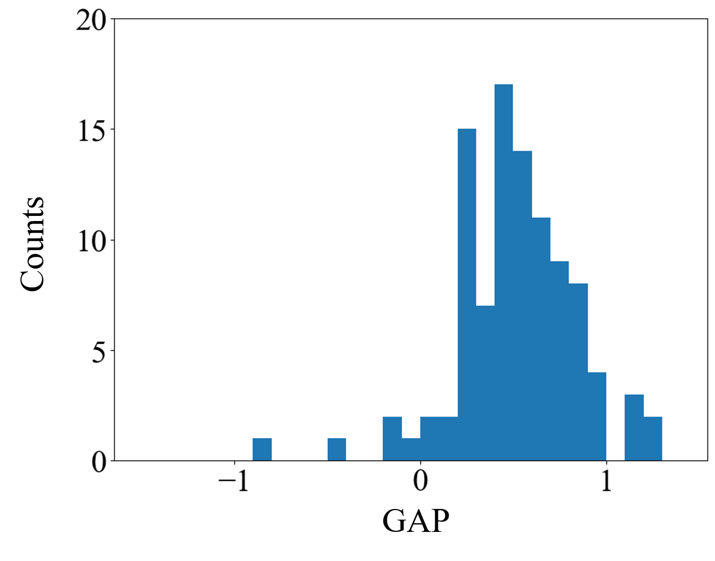
(a) GAPs of Prophet Predictions

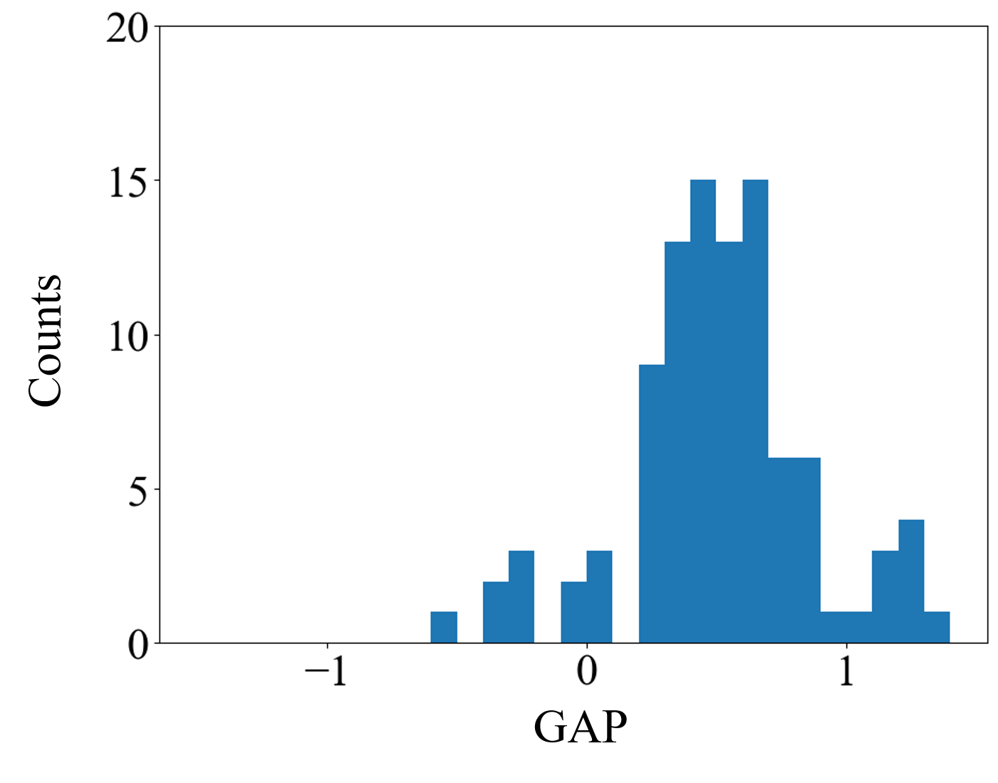
(b) GAPs of ARIMA Predictions

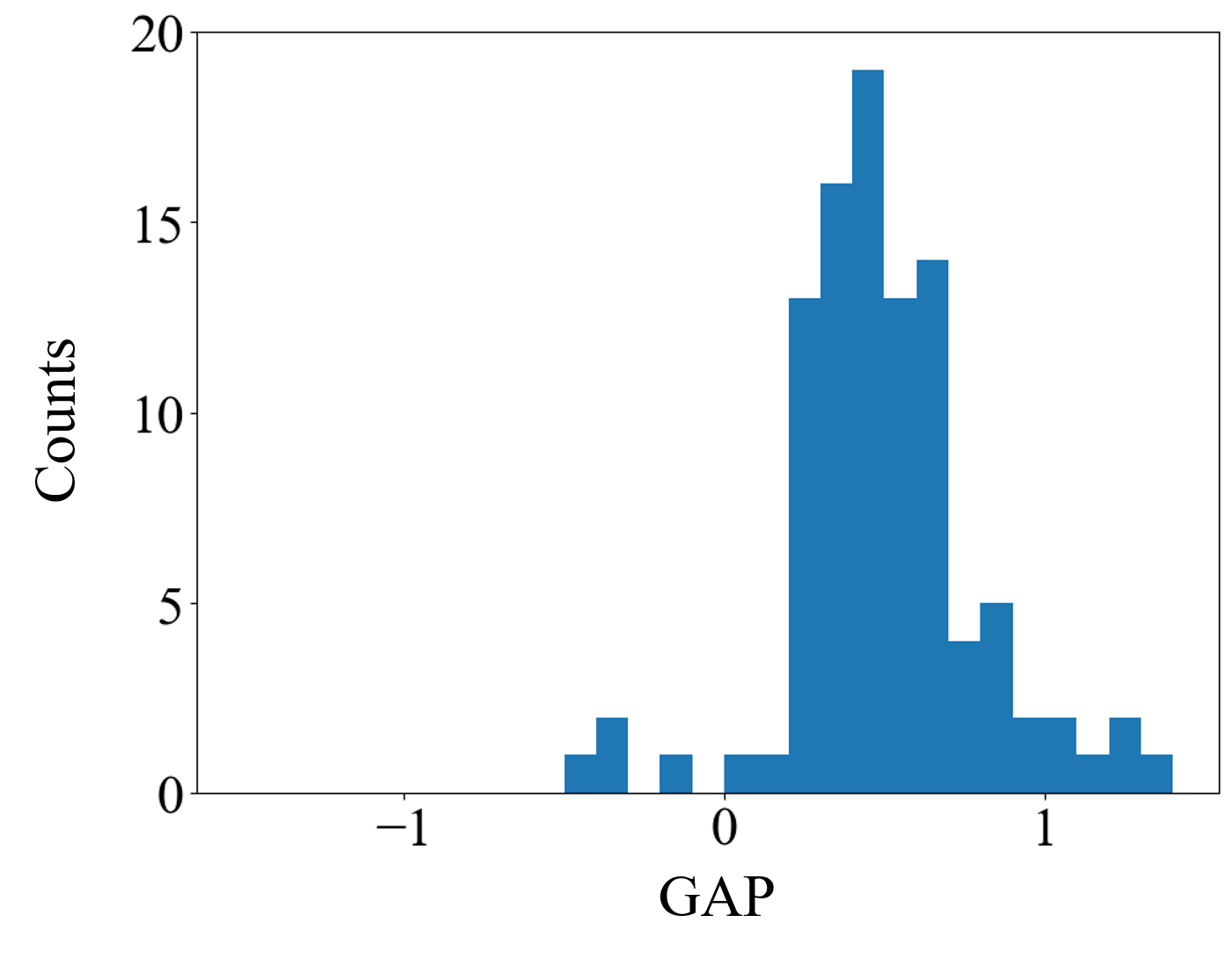
(c) GAPs of Exponential Smoothing Predictions

Figure 1. Histograms of GAPs with different forecasting methods, each containing 100 instances.

6. Conclusion

In this paper, we proposed a new model incorporating predictions into the Online Resource Allocation Problem. With the notion of prediction, we first gave two separate algorithms for the stochastic arrival model and the adversarial arrival model. Under the stochastic arrival model the respective algorithm achieves nearly optimal minimax worst-cast regret, and under the adversarial arrival model the respective algorithm obtains nearly optimal amount of reward. Both algorithms do not need to know the prediction quality beforehand. We then built on these two algorithms and proposed our main algorithm, which achieves the above-mentioned performance under respective arrival models without knowing the underlying arrival model and the prediction quality a priori. The main idea behind our algorithm is to first assume the arrivals are stochastic, while keeps running hypothesis tests on the arrivals to see if the arrivals are adversarial instead.

Appendix A Preliminary Results

We first state two structural results regarding the duality of the offline problem.

Lemma A.1 (Weak Duality).

$\textup{OPT}(\vec{\gamma})\leq D(\mu\mid\vec{\gamma})$ for every $\mu\in\mathbb{R}^{m}_{+}$.

Lemma A.2 (Duality Gap).

$\min_{\mu\in\mathbb{R}^{m}_{+}}D(\mu\mid\vec{\gamma})\leq\textup{OPT}(\vec{\gamma})+(m+1)\overline{r}$.

Lemma A.1 is the standard weak duality result. Lemma A.2 states that, even without any convexity assumptions, the duality gap of our problem is upper bounded by a constant that is independent from the time horizon $T$. This can be shown via Shapley-Folkman Theorem (see Proposition 5.26 of Bertsekas (2014) for a detailed explanation).

Proof of Lemma A.1..

This proof appears in Balseiro et al. (2023). We include it for the sake of completeness. It holds for any $\mu\in\mathbb{R}_{+}^{m}$ that

$$\text{OPT}(\vec{\gamma}) =\left[\begin{array}[]{cc}\max_{x_{t}\in\mathcal{X}_{t}}&\sum_{t=1}^{T}r_{t}\left(x_{t}\right)\\ \text{ s.t. }&\sum_{t=1}^{T}g_{t}\left(x_{t}\right)\leq\rho T\end{array}\right]$$

$$\leq\max_{x_{t}\in\mathcal{X}}\left\{\sum_{t=1}^{T}r_{t}\left(x_{t}\right)+\mu^{\top}\rho T-\mu^{\top}\sum_{t=1}^{T}g_{t}\left(x_{t}\right)\right\}$$

$$=\sum_{t=1}^{T}r_{t}^{*}(\mu)+T\mu^{\top}\rho T$$

$$=D(\mu\mid\vec{\gamma}),$$

where the first inequality is because we relax the constraint $\sum_{t=1}^{T}g_{t}\left(x_{t}\right)\leq\rho T$ and $\mu\geq 0$, and the last equality utilizes the definition of $r^{*}(\cdot)$. ∎

Proof of Proposition 2.1..

Let $\text{conv}(\mathcal{X}_{t})\subset\mathbb{R}^{d}_{+}$ denote the convex hull of $\mathcal{X}_{t}$. For each $t$, define the function $\tilde{r}_{t}:\text{conv}(\mathcal{X}_{t})\to\mathbb{R}_{+}$ by

$$\tilde{r}_{t}(\tilde{x})=\sup\left\{\sum_{k=1}^{d+1}\alpha^{k}r_{t}\left(x^{k}\right)\mid\tilde{x}=\sum_{k=1}^{d+1}\alpha^{k}x^{k},x^{k}\in\mathcal{X}_{t},\sum_{k=1}^{d+1}\alpha^{k}=1,\alpha^{k}\geq 0\right\}\qquad\forall\tilde{x}\in\text{conv}(\mathcal{X}_{t}).$$

$\tilde{r}_{t}$ is concave regardless of whether $r_{t}$ is concave or not, and it can be viewed as a “concavification” of $r_{t}$ on $\text{conv}(\mathcal{X}_{t})$. Similarly, for each $t$, define the function $\tilde{g}_{t}:\text{conv}(\mathcal{X}_{t})\to\mathbb{R}_{+}^{m}$ by

$$\tilde{g}_{t}(\tilde{x})=\inf\left\{\sum_{k=1}^{d+1}\alpha^{k}g_{t}\left(x^{k}\right)\mid\tilde{x}=\sum_{k=1}^{d+1}\alpha^{k}x^{k},x^{k}\in\mathcal{X}_{t},\sum_{k=1}^{d+1}\alpha^{k}=1,\alpha^{k}\geq 0\right\}\qquad\forall\tilde{x}\in\text{conv}(\mathcal{X}_{t}).$$

$\tilde{g}_{t}$ is convex regardless of whether $g_{t}$ is convex or not.

Let $(\text{P})$ denote the optimization problem in Eq. 2.1. Consider the following convex relaxation $(\tilde{\text{P}})$ of the optimization problem in Eq. 2.1:

$$\max_{x_{t}\in\text{conv}(\mathcal{X}_{t})}\sum_{t=1}^{T}\tilde{r}_{t}(\tilde{x}_{t})\quad\text{ s.t. }\quad\sum_{t=1}^{T}\tilde{g}_{t}(\tilde{x}_{t})\leq\rho T;$$

and its Lagrangian dual problem $(\tilde{\text{D}})$:

$$\min_{\mu\in\mathbb{R}_{+}^{m}}\sum_{t=1}^{T}\tilde{r}^{*}_{t}(\tilde{x}_{t})+\mu^{\top}\rho T\quad\text{ where }\quad r^{*}_{t}(\mu)=\sup_{x\in\text{conv}(\mathcal{X}_{t})}\{r_{t}(\tilde{x})-\mu^{\top}\tilde{g}_{t}(\tilde{x})\}.$$

Because $0\in\text{conv}(\mathcal{X}_{t})$, $\tilde{g}_{t}(0)=0$ for all $t$, and $\rho>0$, $(\tilde{\text{P}})$ satisfies Slater’s condition. Therefore by strong duality $\sup(\tilde{\text{P}})=\inf(\tilde{\text{D}})$. By an application of the Sharpley-Folkman Theorem (Bertsekas (2014), Proposition 5.26), there exists an optimal solution $\{\tilde{x}^{*}_{t}\}_{t=1}^{T}$ of $(\tilde{\text{P}})$ with the following property: let $I\subset[T]$ be the set of time periods where $\tilde{x}^{*}_{t}\notin\mathcal{X}_{t}$ for $t\in I$, then $|I|\leq m+1$ and $\sum_{t\in[T]\setminus I}g_{t}(\tilde{x}^{*}_{t})\leq\rho T$. Let $\tilde{\mu}^{*}$ be the optimal dual variable of $(\tilde{\text{D}})$ that induces $\{\tilde{x}^{*}_{t}\}_{t=1}^{T}$, and let $\{x^{\tilde{\mu}^{*}}_{t}\}_{t=1}^{T}$ be the actions induced by $\tilde{\mu}^{*}$ in the original primal $(\text{P})$. We prove that $\sum_{t=1}^{T}r_{t}(x^{\tilde{\mu}^{*}}_{t})\geq\sum_{t=1}^{T}r_{t}(\tilde{x}^{*}_{t})-(\bar{g}/\underline{g}+1)(m+1)\bar{r}$.

Let $S\subset[T]$ be the set of time periods such that $x^{\tilde{\mu}^{*}}_{s}\neq\tilde{x}^{*}_{s}$ for $s\in S$, and let $J=S\setminus I$. Then $J$ is the set of time periods where the resource constraint becomes active when choosing the action induced by $\tilde{\mu}^{*}$. Because $|I|\leq m+1$ and $x^{\tilde{\mu}^{*}}_{t}=\tilde{x}^{*}_{t}$ for $t\in[T]\setminus S$, $\sum_{t\in J}g_{t}(\tilde{x}^{*}_{t})-\sum_{t\in J}g_{t}(x^{\tilde{\mu}^{*}}_{t})\leq(m+1)\bar{g}$. Therefore $|\{t\in J:\tilde{x}^{*}_{t}\neq 0\}|\leq(m+1)\bar{g}/\underline{g}$, so $\sum_{t\in J}r_{t}(\tilde{x}^{*}_{t})-\sum_{t\in J}r_{t}(x^{\tilde{\mu}^{*}}_{t})\leq(m+1)\bar{r}\bar{g}/\underline{g}$. Further, we also have $\sum_{t\in I}r_{t}(\tilde{x}^{*}_{t})-\sum_{t\in I}r_{t}(x^{\tilde{\mu}^{*}}_{t})\leq(m+1)\bar{r}$ and $x^{\tilde{\mu}^{*}}_{t}=\tilde{x}^{*}_{t}$ for $t\in[T]\setminus S$. These together gives $\sum_{t=1}^{T}r_{t}(x^{\tilde{\mu}^{*}}_{t})\geq\sum_{t=1}^{T}r_{t}(\tilde{x}^{*}_{t})-(\bar{g}/\underline{g}+1)(m+1)\bar{r}$. Finally, since $(\tilde{\text{P}})$ is a relaxation of $(\text{P})$, $\sup(\tilde{\text{P}})=\sum_{t=1}^{T}r_{t}(\tilde{x}^{*}_{t})\geq\text{OPT}(\vec{\gamma})$, so we have $\sum_{t=1}^{T}r_{t}(x^{\tilde{\mu}^{*}}_{t})\geq\text{OPT}(\vec{\gamma})-(\bar{g}/\underline{g}+1)(m+1)\bar{r}$. The result follows by our definition of $\mu^{*}$, which ensures $\sum_{t=1}^{T}r_{t}(x^{\mu^{*}}_{t})\geq\sum_{t=1}^{T}r_{t}(x^{\tilde{\mu}^{*}}_{t})$. ∎

Appendix B Proofs in Section 4.1 and 4.2

Proof of Theorem 4.1..

The proof technique is similar to the proof of Theorem 1 in Balseiro et al. (2023), which we largely borrow. We break down the proof in three steps.
Step 1 (Primal performance.) First, we define the stopping time $\tau_{A}$ of Algorithm 3 as the first time less than $T$ that there exists resource $j$ such that $\sum_{t=1}^{\tau_{A}}\left(g_{t}\left(x_{t}\right)\right)_{j}+\bar{g}\geq\rho_{j}T$. Notice that $\tau_{A}$ is a random variable, and moreover, we will not violate the resource constraints before the stopping time $\tau_{A}$. We here study the primal-dual gap until the stopping-time $\tau_{A}$. Notice that before the stopping time $\tau_{A}$, Algorithm 3 performs the mirror descent steps on the dual function with fine-tuned step sizes.

Consider a time $t\leq\tau_{A}$ so that actions are not constrained by resources. Then the algorithm takes the action $x_{t}\in\arg\max_{x\in\mathcal{X}_{t}}\left\{r_{t}(x)-\right.$ $\left.\mu_{t}^{\top}g_{t}(x)\right\}$, so we have that

$$r_{t}\left(x_{t}\right)=r_{t}^{*}\left(\mu_{t}\right)+\mu_{t}^{\top}g_{t}\left(x_{t}\right).$$

Let $\bar{D}(\mu\mid\mathcal{P})=\frac{1}{T}\mathbb{E}_{\vec{\gamma}\sim\mathcal{P}^{T}}[D(\mu\mid\vec{\gamma})]=\mathbb{E}_{(r,g,\mathcal{X})\sim\mathcal{P}}\left[r^{*}\left(\mu_{t}\right)\right]+\mu_{t}^{\top}\rho$ be the expected dual objective at $\mu$ when requests are drawn i.i.d. from $\mathcal{P}\in\Delta(\mathcal{S})$. Let $\xi_{t}=\left\{\gamma_{0},\ldots,\gamma_{t}\right\}$ and $\sigma\left(\xi_{t}\right)$ be the sigma-algebra generated by $\xi_{t}$. Adding the last two equations and taking expectations conditional on $\sigma\left(\xi_{t-1}\right)$ we obtain, because $\mu_{t}\in\sigma\left(\xi_{t-1}\right)$ and $\left(r_{t},g_{t},\mathcal{X}_{t}\right)\sim\mathcal{P}$, that

(B.1) $$\mathbb{E}\left[r_{t}\left(x_{t}\right)\mid\sigma\left(\xi_{t-1}\right)\right] = \mathbb{E}_{(r,g,\mathcal{X})\sim\mathcal{P}}\left[f^{*}\left(\mu_{t}\right)\right]+\mu_{t}^{\top}\rho+\mu_{t}^{\top}\left(\mathbb{E}\left[g_{t}\left(x_{t}\right)\mid\sigma\left(\xi_{t-1}\right)\right]-\rho\right)$$

$$= \bar{D}\left(\mu_{t}\mid\mathcal{P}\right)-\mathbb{E}\left[\mu_{t}^{\top}\left(\rho-g_{t}\left(x_{t}\right)\right)\mid\sigma\left(\xi_{t-1}\right)\right]$$

where the second equality follows the definition of the dual function.

Consider the process $Z_{t}=\sum_{s=1}^{t}\mu_{s}^{\top}\left(a_{s}-b_{s}\left(x_{s}\right)\right)-\mathbb{E}\left[\mu_{s}^{\top}\left(a_{s}-b_{s}\left(x_{s}\right)\right)\mid\sigma\left(\xi_{s-1}\right)\right]$, which is martingale with respect to $\xi_{t}$ (i.e., $Z_{t}\in\sigma\left(\xi_{t}\right)$ and $\mathbb{E}\left[Z_{t+1}\mid\sigma\left(\xi_{t}\right)\right]=Z_{t}$ ). Since $\tau_{A}$ is a stopping time with respect to $\xi_{t}$ and $\tau_{A}$ is bounded, the Optional Stopping Theorem implies that $\mathbb{E}\left[Z_{\tau_{A}}\right]=0$. Therefore,

$$\mathbb{E}\left[\sum_{t=1}^{\tau_{A}}\mu_{t}^{\top}\left(\rho-g_{t}\left(x_{t}\right)\right)\right]=\mathbb{E}\left[\sum_{t=1}^{\tau_{A}}\mathbb{E}\left[\mu_{t}^{\top}\left(\rho-g_{t}\left(x_{t}\right)\right)\mid\sigma\left(\xi_{t-1}\right)\right]\right].$$

Using a similar martingale argument for $f_{t}\left(x_{t}\right)$ and summing (9) from $t=1,\ldots,\tau_{A}$ we obtain that

(B.2) $$\mathbb{E}\left[\sum_{t=1}^{\tau_{A}}r_{t}\left(x_{t}\right)\right] = \mathbb{E}\left[\sum_{t=1}^{\tau_{A}}\bar{D}\left(\mu_{t}\mid\mathcal{P}\right)\right]-\mathbb{E}\left[\sum_{t=1}^{\tau_{A}}\mu_{t}^{\top}\left(\rho-g_{t}\left(x_{t}\right)\right)\right]$$

$$\geq \mathbb{E}\left[\tau_{A}\bar{D}\left(\bar{\mu}_{\tau_{A}}\mid\mathcal{P}\right)\right]-\mathbb{E}\left[\sum_{t=1}^{\tau_{A}}\mu_{t}^{\top}\left(\rho-g_{t}\left(x_{t}\right)\right)\right].$$

where the inequality follows from denoting $\bar{\mu}_{\tau_{A}}=\frac{1}{\tau_{A}}\sum_{t=1}^{\tau_{A}}\mu_{t}$ to be the average dual variable and using that the dual function is convex.

Step 2 (Complementary slackness). Consider the sequence of functions $w_{t}(\mu)=\mu^{\top}\left(\rho-g_{t}\left(x_{t}\right)\right)$, which capture the complementary slackness at time $t$. The sub-gradients are given by $\nabla_{\mu}w_{t}(\mu)=\rho-g_{t}\left(x_{t}\right)$, which are bounded as follows $\left\|\nabla_{\mu}w_{t}(\mu)\right\|_{\infty}\leq\left\|g_{t}\left(x_{t}\right)\right\|_{\infty}+\|\rho\|_{\infty}\leq\bar{g}+\bar{\rho}$. Therefore, Algorithm 3 applies online mirror descent to the sequence of functions $w_{t}(\mu)$ with the fine-tuned step sizes. To analyze the performance, we use the following lemma from Carmon & Hinder (2022).

Lemma B.1 (Theorem 4 in Carmon & Hinder (2022)).

Under the assumptions and notations of our paper, the online mirror descent in Algorithm 3 with the proposed step sizes satisfies, with probability at least $1-\frac{1}{T}$, that

$$\sum_{t=1}^{\tau_{A}}\left(w_{t}\left(\mu_{t}\right)-w_{t}(\mu^{*})\right)\leq CT^{\frac{1}{2}}||\mu_{1}-\mu^{*}||_{1}\cdot\textup{polylog}(T)$$

where $C>0$ is some constant.

Because $||\mu_{1}-\mu^{*}||_{1}=||\hat{\mu}-\mu^{*}||_{1}\leq\kappa T^{-a}$, Lemma B.1 states that $\sum_{t=1}^{\tau_{A}}w_{t}\left(\mu_{t}\right)-w_{t}(\mu^{*})\leq\kappa CT^{\frac{1}{2}-a}\cdot\textup{polylog}(T)$ with probability at least $1-\frac{1}{T}$.

Step 3 (Putting it all together). For any $\mathcal{P}\in\Delta(\mathcal{S})$ and $\tau_{A}\in[0,T]$ we have that

(B.3) $$\mathbb{E}_{\vec{\gamma}\sim\mathcal{P}^{T}}[\mathrm{OPT}(\vec{\gamma})]=\frac{\tau_{A}}{T}\mathbb{E}_{\vec{\gamma}\sim\mathcal{P}^{T}}[\mathrm{OPT}(\vec{\gamma})]+\frac{T-\tau_{A}}{T}\mathbb{E}_{\vec{\gamma}\sim\mathcal{P}^{T}}[\mathrm{OPT}(\vec{\gamma})]\leq\tau_{A}\bar{D}\left(\bar{\mu}_{\tau_{A}}\mid\mathcal{P}\right)+\left(T-\tau_{A}\right)\bar{r},$$

where the inequality uses Lemma A.1 and the fact that $\text{OPT}(\vec{\gamma})\leq\bar{r}T$. Therefore, with probability at least $1-\frac{1}{T}$,

(B.4) $$\text{Regret}(\text{SA}\mid\mathcal{P}) = \mathbb{E}_{\vec{\gamma}\sim\mathcal{P}^{T}}[\text{OPT}(\vec{\gamma})-R(\text{SA}\mid\vec{\gamma})]$$

$$\leq \mathbb{E}_{\vec{\gamma}\sim\mathcal{P}^{T}}\left[\text{OPT}(\vec{\gamma})-\sum_{t=1}^{\tau_{A}}r_{t}\left(x_{t}\right)\right]$$

$$\leq \mathbb{E}_{\vec{\gamma}\sim\mathcal{P}^{T}}\left[\text{OPT}(\vec{\gamma})-\tau_{A}D\left(\bar{\mu}_{\tau_{A}}\mid\mathcal{P}\right)+\sum_{t=1}^{\tau_{A}}w_{t}\left(\mu_{t}\right)\right]$$

$$\leq \mathbb{E}_{\vec{\gamma}\sim\mathcal{P}^{T}}\left[\textup{OPT}(\vec{\gamma})-\tau_{A}D\left(\bar{\mu}_{\tau_{A}}\mid\mathcal{P}\right)+\sum_{t=1}^{\tau_{A}}w_{t}(\mu^{*})+CT^{\frac{1}{2}-a}\cdot\textup{polylog}(T)\right]$$

$$\leq \mathbb{E}_{\vec{\gamma}\sim\mathcal{P}^{T}}\underbrace{\left[\left(T-\tau_{A}\right)\cdot\bar{r}+\sum_{t=1}^{\tau_{A}}w_{t}(\mu^{*})+CT^{\frac{1}{2}-a}\cdot\textup{polylog}(T)\right]}_{\clubsuit}$$

where the first inequality follows from using that $\tau_{A}\leq T$ together with $r_{t}(\cdot)\geq 0$ to drop all requests after $\tau_{A}$; the second is from Eq. (B.2); the third follows from Lemma B.1; and the last from Eq. (B.3).

Note that $\sum_{t=1}^{\tau_{A}}w_{t}(\mu^{*})\leq\sum_{t=1}^{\tau_{A}}w_{t}(\mu)$ for every $\mu\in\mathbb{R}_{+}^{m}$. We now discuss the choice of $\mu\in\mathbb{R}_{+}^{m}$ in order to upper bound $\sum_{t=1}^{\tau_{A}}w_{t}(\mu^{*})$. If $\tau_{A}=T$, then set $\mu=0$ to obtain that $\clubsuit\leq CT^{\frac{1}{2}-a}\cdot\textup{polylog}(T)$. If $\tau_{A}<T$, then there exists a resource $j\in[m]$ such that $\sum_{t=1}^{\tau_{A}}\left(g_{t}\left(x_{t}\right)\right)_{j}+\bar{g}\geq\rho_{j}T$. Set $\mu=\left(\bar{r}/\rho_{j}\right)e_{j}$ with $e_{j}$ being the $j$-th unit vector. This yields

$$\sum_{t=1}^{\tau_{A}}w_{t}(\mu^{*})\leq\sum_{t=1}^{\tau_{A}}w_{t}(\mu)=\sum_{t=1}^{\tau_{A}}\mu^{\top}\left(\rho-g_{t}\left(x_{t}\right)\right)$$

$$= \frac{\bar{r}}{\rho_{j}}\sum_{t=1}^{\tau_{A}}\left(\rho_{j}-\left(g_{t}\left(x_{t}\right)\right)_{j}\right)\leq\frac{\bar{r}}{\rho_{j}}\left(\tau_{A}\rho_{j}-\rho_{j}T+\bar{g}\right)=\frac{\bar{r}}{\rho_{j}}\bar{g}-\bar{r}\left(T-\tau_{A}\right),$$

where the inequality follows because of the definition of the stopping time $\tau_{A}$. Therefore, using that $\rho_{j}\geq\underline{\rho}$ for every resource $j\in[m]$, we have

$$\clubsuit\leq\frac{\bar{r}\bar{g}}{\underline{\rho}}+CT^{\frac{1}{2}-a}\cdot\textup{polylog}(T).$$

Therefore $\text{Regret}(\text{SA})\leq\frac{\bar{r}\bar{g}}{\underline{\rho}}+CT^{\frac{1}{2}-a}\cdot\textup{polylog}(T)$ with probability at least $1-\frac{1}{T}.$ We conclude by noting that $\text{Regret}(\text{SA})\leq\mathbb{E}_{\vec{\gamma}\sim\mathcal{P}^{T}}[\text{OPT}(\vec{\gamma})]\leq\bar{r}T$, so we have $\text{Regret}(\text{SA})\leq\frac{\bar{r}\bar{g}}{\underline{\rho}}+\bar{r}+CT^{\frac{1}{2}-a}\cdot\textup{polylog}(T)\in\tilde{O}(\max\{T^{\frac{1}{2}-a},1\})$. ∎

Proof of Theorem 4.2..

By Assumption 2.2, there exists a function $\psi(T)$ such that $||\hat{\mu}-\mu^{*}||_{1}\leq\psi(T)$ and $\psi(T)=o(\epsilon(T))$. We break down the proof into two lemmas, which compares $R(\textup{AA}\mid\vec{\gamma})$ with $\frac{1}{\alpha^{*}}\textup{OPT}(\vec{\gamma})$ and $R(\textup{PRD}\mid\vec{\gamma})$ separately.

Lemma B.2.

Consider the Adversarial Arrival Algorithm (AA) under the adversarial arrival model. Given a prediction $\hat{\mu}$ with accuracy parameter $a$, it holds that:

$$\limsup_{T\to\infty}\sup_{\vec{\gamma}\in\mathcal{S}^{T}}\left\{\frac{1}{T}\left(\frac{1}{\alpha^{*}}\textup{OPT}(\vec{\gamma})-R(\textup{AA}\mid\vec{\gamma})\right)\right\}\leq 0.$$

Proof of Lemma B.2..

The proof is drawn from the proof of Theorem 2 in Balseiro et al. (2023). The proof contains three steps, which is similar to the proof of Theorem 4.1.
Step 1 (Primal performance.) Fix an arrival sequence $\vec{\gamma}\in\mathcal{S}^{T}$ and let $x^{*}\in\mathcal{X}_{t}$ be an optimal action in $\text{OPT}(\vec{\gamma})$ at time $t$. Let $\tau_{A}$ be the stopping time of Algorithm 4, which is defined similarly as in the proof of Theorem 4.1, then for $t\leq\tau_{A}$ we have $x_{t}\in\arg\max_{x\in\mathcal{X}_{t}}\left\{r_{t}(x)-\mu_{t}^{\top}g_{t}(x)\right\}$, and thus $r_{t}\left(x_{t}\right)\geq r_{t}\left(x_{t}^{*}\right)-\mu_{t}^{\top}\left(g_{t}\left(x_{t}^{*}\right)-g_{t}\left(x_{t}\right)\right)$ and $0=r_{t}(0)\leq r_{t}\left(x_{t}\right)-\mu_{t}^{\top}g_{t}\left(x_{t}\right)$. Therefore

$$\alpha^{*}r_{t}\left(x_{t}\right) = r_{t}\left(x_{t}\right)+(\alpha^{*}-1)r_{t}\left(x_{t}\right)$$

$$\geq r_{t}\left(x_{t}^{*}\right)+\mu_{t}^{\top}g_{t}\left(x_{t}\right)-\mu_{t}^{\top}g_{t}\left(x_{t}^{*}\right)+(\alpha^{*}-1)\left(\mu_{t}^{\top}g_{t}\left(x_{t}\right)\right)$$

$$= r_{t}\left(x_{t}^{*}\right)-\alpha^{*}\mu_{t}^{\top}\left(\rho-g_{t}\left(x_{t}\right)\right)+\alpha^{*}\mu_{t}^{\top}\rho-\mu_{t}^{\top}g_{t}\left(x_{t}^{*}\right)$$

$$\geq r_{t}\left(x_{t}^{*}\right)-\alpha^{*}\mu_{t}^{\top}\left(\rho-g_{t}\left(x_{t}\right)\right),$$

where the second inequality is because $\alpha^{*}\mu_{t}^{\top}\rho-\mu_{t}^{\top}g_{t}\left(x_{t}^{*}\right)\geq 0$ by our definition of $\alpha^{*}$ and the fact that $\mu_{t}\geq 0$. Summing up over $t=1,\ldots,\tau_{A}$ yields

(B.5) $$\alpha^{*}\sum_{t=1}^{\tau_{A}}r_{t}\left(x_{t}\right)\geq\sum_{t=1}^{\tau_{A}}r_{t}\left(x_{t}^{*}\right)-\alpha^{*}\sum_{t=1}^{\tau_{A}}\mu_{t}^{\top}\left(\rho-g_{t}\left(x_{t}\right)\right).$$

Step 2 (Complementary slackness). Denoting, as before, $w_{t}(\mu)=\mu^{\top}\left(\rho-b_{t}\left(x_{t}\right)\right)$. As we have seen in the step 2 in the proof of Theorem 4.1 (the analysis is deterministic in nature), Algorithm 4 performs online mirror descent to the sequence of functions $w_{t}(\mu)$ with step size $\eta=c\epsilon(T)/T$ where $c>0$ is an arbitrary scaling constant. By our assumption that the reference function $h(\cdot)$ is Lipschitz, there exists a constant $L>0$ such that $V_{h}(\mu^{\prime},\mu^{\prime\prime})\leq L||\mu^{\prime}-\mu^{\prime\prime}||_{1}$ for all $\mu^{\prime},\mu^{\prime\prime}\in\mathbb{R}^{m}_{+}$. By a standard result on online mirror descent (see, e.g., Appendix G of Balseiro et al. (2023)), we have

(B.6) $$\sum_{t=1}^{\tau_{A}}w_{t}(\mu_{t}) \leq \sum_{t=1}^{\tau_{A}}w_{t}(\mu^{*})+\frac{(\bar{g}+\bar{\rho})^{2}\eta}{2\sigma}\tau_{A}+\frac{1}{\eta}V_{h}(\mu^{*},\mu_{1})$$

$$\leq \sum_{t=1}^{\tau_{A}}w_{t}(\mu^{*})+\frac{c(\bar{g}+\bar{\rho})^{2}}{2\sigma}\epsilon(T)+\frac{\kappa L\psi(T)T}{c\epsilon(T)},$$

where the first inequality is the standard online mirror descent result, and the second inequality follows by the step size $\eta=c\epsilon(T)/T$ and the fact that $||\mu_{1}-\mu^{*}||_{1}=||\hat{\mu}-\mu^{*}||_{1}\leq\psi(T)$.

Step 3 (Putting it all together). We have

$$\operatorname{OPT}(\vec{\gamma})-\alpha R(\text{AA}\mid\vec{\gamma}) \leq\sum_{t=1}^{T}r_{t}\left(x_{t}^{*}\right)-\alpha^{*}\sum_{t=1}^{\tau_{A}}r_{t}\left(x_{t}\right)$$

$$\leq\sum_{t=\tau_{A}+1}^{T}r_{t}\left(x_{t}^{*}\right)+\alpha^{*}\sum_{t=1}^{\tau_{A}}w_{t}\left(\mu_{t}\right)$$

$$\leq\left(T-\tau_{A}\right)\cdot\bar{r}+\alpha^{*}\sum_{t=1}^{\tau_{A}}w_{t}(\mu^{*})+\alpha^{*}\left(\frac{c(\bar{g}+\bar{\rho})^{2}}{2\sigma}\epsilon(T)+\frac{\kappa L\psi(T)T}{c\epsilon(T)}\right),$$

where the first inequality follows because $\tau_{A}\leq T$ and $r_{t}(\cdot)\geq 0$, the second inequality is from Eq. (B.5), and the third inequality utilizes $r_{t}\left(x_{t}^{*}\right)\leq\bar{r}$ and Eq. (B.6). Similar to the proof of Theorem 4.1, we note that $\sum_{t=1}^{\tau_{A}}w_{t}(\mu^{*})\leq\sum_{t=1}^{\tau_{A}}w_{t}(\mu)$ for every $\mu\in\mathbb{R}_{+}^{m}$ and discuss the choice of $\mu\in\mathbb{R}_{+}^{m}$ in order to upper bound $\sum_{t=1}^{\tau_{A}}w_{t}(\mu^{*})$. If $\tau_{A}=T$, then set $\mu=0$, and the result follows. If $\tau_{A}<T$, then there exists a resource $j\in[m]$ such that $\sum_{t=1}^{\tau_{A}}\left(g_{t}\left(x_{t}\right)\right)_{j}+\bar{g}\geq\rho_{j}T$. Set $\mu=\left(\bar{r}/\left(\alpha^{*}\rho_{j}\right)\right)e_{j}$ where $e_{j}$ is the $j$-th unit vector and repeat the steps of the stochastic arrivals case to obtain:

$$\operatorname{OPT}(\vec{\gamma})-\alpha^{*}R(\text{AA}\mid\vec{\gamma})\leq\frac{\bar{r}\bar{g}}{\underline{\rho}}+\alpha^{*}\left(\frac{c(\bar{g}+\bar{\rho})^{2}}{2\sigma}\epsilon(T)+\frac{\kappa L\psi(T)T}{c\epsilon(T)}\right),$$

which finishes the proof by noticing that $\epsilon(T)$ and $\psi(T)T/\epsilon(T)$ are both sub-linear in $T$. ∎

Lemma B.3.

Consider the Adversarial Arrival Algorithm (AA) under the adversarial arrival model. Given a prediction $\hat{\mu}$ with accuracy parameter $a$, it holds that:

$$\limsup_{T\to\infty}\sup_{\vec{\gamma}\in\mathcal{S}^{T}}\left\{\frac{1}{T}\left(R(\textup{PRD}\mid\vec{\gamma})-R(\textup{AA}\mid\vec{\gamma})\right)\right\}\leq 0.$$

Proof of Lemma B.3..

Recall the updating rule $\mu_{t+1}\in\arg\min_{\mu\in\mathbb{R}_{+}^{m}}\phi_{t}^{\top}\mu+\frac{1}{\eta}V_{h}\left(\mu,\mu_{t}\right)$ where $\phi_{t}=-g_{t}(x_{t})+\rho$. Note that $\phi_{t}^{\top}\mu+\frac{1}{\eta}V_{h}\left(\mu,\mu_{t}\right)$ is convex in $\mu$, and set its gradient of $\mu$ to zero yields $\phi_{t}+\frac{1}{\eta}(\nabla h(\mu)-\nabla h(\mu_{t}))=0$, where $h(\cdot)$ is the reference function. Because $||\phi_{t}||_{\infty}\leq||g_{t}(x_{t})||_{\infty}+||\rho||_{\infty}\leq\bar{g}+\bar{\rho}$ and by our assumption $h(\cdot)$ is $\sigma$-strongly convex with respect to the $\ell_{1}$-norm in $\mathbb{R}^{m}_{+}$, we have $||\mu_{t+1}-\mu_{t}||_{1}\leq\frac{\eta}{\sigma}||\phi_{t}||_{\infty}\leq\frac{c(\bar{g}+\bar{\rho})\epsilon(T)}{\sigma T}$. Therefore $||\mu_{t}-\hat{\mu}||_{1}=||\mu_{t}-\mu_{1}||_{1}\leq\sum_{s=2}^{t}||\mu_{s}-\mu_{s-1}||_{1}\leq\frac{c(\bar{g}+\bar{\rho})\epsilon(T)}{\sigma T}t$, and hence

(B.7) $$\sum_{t=1}^{T}||\mu_{t}-\hat{\mu}||_{1}\leq\left(\frac{c(\bar{g}+\bar{\rho})}{2\sigma}+1\right)\epsilon(T).$$

Let $x_{t}^{\hat{\mu}}$ be the actions taken by the Prediction Algorithm at time $t$, then $R(\textup{PRD}\mid\vec{\gamma})=\sum_{t=1}^{T}r_{t}(x_{t}^{\hat{\mu}})$. Because $\zeta>0$ is a constant and $\epsilon(T)\in o(1)$, $||\mu_{t}-\hat{\mu}||_{1}\leq\frac{c(\bar{g}+\bar{\rho})\epsilon(T)}{\sigma T}t\leq\zeta$ for all $t$ as $T\to\infty$. Therefore $\mu_{1},\dots,\mu_{T}$ is a sequence of dual variables that satisfies Assumption 2.1. Let $\tau_{A}^{j}$ be the depletion time of resources $j$ of Algorithm 4 and $\tau_{P}^{j}$ be the depletion time of resources $j$ of Algorithm 1. Then by Assumption 2.2 we have $|\tau_{P}^{j}-\tau_{A}^{j}|\in o(T)$ for all resource $j$. Moreover, since there are $m$ resources, outside of all times between each $\tau_{A}^{j}$ and $\tau_{P}^{j}$, $T$ is partitioned into at most $m+1$ consecutive time blocks, say $B_{1},\dots,B_{k}$ for some $k\leq m+1$. Note that the set of feasible actions $\{x\mid,x\in\mathcal{X}_{t},g_{t}(x)\leq\text{amount of remaining resources}\}$ at time period $t$ is the same for Algorithm 4 and Algorithm 1 for all $t\in\cup_{k^{\prime}=1}^{k}B_{k^{\prime}}$. Therefore both algorithms perform online mirror descent during time periods $B_{1},\dots,B_{k}$. Therefore similar to Eq. (B.6) we have

(B.8) $$\sum_{t\in B_{k^{\prime}}}w_{t}(\mu_{t})\leq\sum_{t\in B_{k^{\prime}}}w_{t}(\hat{\mu})+\frac{c(\bar{g}+\bar{\rho})^{2}}{2\sigma}\epsilon(T)+\frac{\kappa L\psi(T)T}{c\epsilon(T)}$$

for each $B_{k^{\prime}}$. Also, because $x_{t}\in\arg\max_{x\in\mathcal{X}_{t},g_{t}(x)\leq G_{t}}\left\{r_{t}(x)-\mu_{t}^{\top}g_{t}(x)\right\}$, for $t\in\cup_{k^{\prime}=1}^{k}B_{k^{\prime}}$ we have

(B.9) $$r_{t}(x_{t})-\mu_{t}^{\top}g_{t}(x_{t})\geq r_{t}(x_{t}^{\hat{\mu}})-\mu_{t}^{\top}g_{t}(x_{t}^{\hat{\mu}}).$$

Because $w_{t}(\mu_{t})=\mu_{t}^{\top}(\rho-g_{t}(x_{t}))$ and $w_{t}(\hat{\mu})=\hat{\mu}^{\top}(\rho-g_{t}(x_{t}^{\hat{\mu}}))$, for each $B_{k}^{\prime}$ we get

$$\sum_{t\in B_{k^{\prime}}}(r_{t}(x_{t}^{\hat{\mu}})-r_{t}(x_{t})) \leq \sum_{t\in B_{k^{\prime}}}(\mu_{t}^{\top}g_{t}(x_{t}^{\hat{\mu}})-\mu_{t}^{\top}g_{t}(x))$$

$$= \sum_{t\in B_{k^{\prime}}}\mu_{t}^{\top}(\rho-g_{t}(x))-\sum_{t\in B_{k^{\prime}}}\hat{\mu}^{\top}(\rho-g_{t}(x_{t}^{\hat{\mu}}))+\sum_{t\in B_{k^{\prime}}}(\hat{\mu}-\mu_{t})^{\top}(\rho-g_{t}(x_{t}^{\hat{\mu}}))$$

$$\leq \sum_{t\in B_{k^{\prime}}}w_{t}(\mu_{t})-\sum_{t\in B_{k^{\prime}}}w_{t}(\hat{\mu})+\bar{\rho}\sum_{t\in B_{k^{\prime}}}||\mu_{t}-\hat{\mu}||_{1}$$

$$\leq \frac{c(\bar{g}+\bar{\rho})^{2}}{2\sigma}\epsilon(T)+\frac{\kappa L\psi(T)T}{c\epsilon(T)}+\left(\frac{c\bar{\rho}(\bar{g}+\bar{\rho})}{2\sigma}+\bar{\rho}\right)\epsilon(T),$$

where the first inequality follows from Eq. (B.9), the second inequality is because by Hölder’s inequality $(\hat{\mu}-\mu_{t})^{\top}(\rho-g_{t}(x_{t}^{\hat{\mu}}))\leq||\hat{\mu}-\mu_{t}||_{1}||\rho-g_{t}(x_{t}^{\hat{\mu}})||_{\infty}\leq\bar{\rho}||\hat{\mu}-\mu_{t}||_{1}$, and the third inequality follows from Eq. (B.8) and Eq. (B.7). Therefore

$$R(\textup{PRD}\mid\vec{\gamma})-R(\textup{AA}\mid\vec{\gamma}) = \sum_{t\in\cup_{k^{\prime}=1}^{k}B_{k^{\prime}}}(r_{t}(x_{t}^{\hat{\mu}})-r_{t}(x_{t}))+\sum_{t\in[T]\setminus\cup_{k^{\prime}=1}^{k}B_{k^{\prime}}}(r_{t}(x_{t}^{\hat{\mu}})-r_{t}(x_{t}))$$

$$\leq k\left(\frac{c(\bar{g}+\bar{\rho})^{2}}{2\sigma}\epsilon(T)+\frac{\kappa L\psi(T)T}{c\epsilon(T)}+\left(\frac{c\bar{\rho}(\bar{g}+\bar{\rho})}{2\sigma}+\bar{\rho}\right)\epsilon(T)\right)$$

$$+\bar{r}\cdot|[T]\setminus\cup_{k^{\prime}=1}^{k}B_{k^{\prime}}|$$

$$= o(T),$$

where the first inequality is because $r_{t}(x_{t}^{\hat{\mu}})-r_{t}(x_{t})\leq\bar{r}$ for each $t$, and the second inequality is by noting that $k\leq m$, $\epsilon(T)=o(T),\psi(T)T/\epsilon(T)=o(T)$, and $|[T]\setminus\cup_{k^{\prime}=1}^{k}B_{k^{\prime}}|\leq\sum_{j=1}^{m}|\tau_{P}^{j}-\tau_{A}^{j}|$. This shows $\limsup_{T\to\infty}\sup_{\vec{\gamma}\in\mathcal{S}^{T}}\left\{\frac{1}{T}\left(R(\textup{PRD}\mid\vec{\gamma})-R(\textup{AA}\mid\vec{\gamma})\right)\right\}\leq 0.$ ∎

Combine Lemma B.2 and Lemma B.3 gives Theorem 4.2. ∎

Appendix C Proofs in Section 4.3

Proof of Theorem 4.3..

We divide the proof into three cases. The first case is that the underlying arrival model is stochastic and the algorithm never switches to the Adversarial Arrival Algorithm (i.e., the “for” loop in the algorithm is never broken), and in this case we show that $\textup{Regret}(\textup{MainALG})=\tilde{O}(\max\{T^{\frac{1}{2}-a},1\})$. The second case is that the underlying arrival model is stochastic and yet the algorithm switches to the Adversarial Arrival Algorithm at some point, and we prove that this case happens with low probability. The third case is that the underlying arrival model is adversarial, and in this case we show that

$$\limsup_{T\to\infty}\sup_{\vec{\gamma}\in\mathcal{S}^{T}}\left\{\frac{1}{T}\left(\max\left\{\frac{1}{\alpha^{*}}\textup{OPT}(\vec{\gamma}),R(\textup{PRD}\mid\vec{\gamma})\right\}-R(\textup{MainALG}\mid\vec{\gamma})-\bar{r}\delta T\right)\right\}\leq 0,$$

regardless of whether the algorithm switches to the Adversarial Arrival Algorithm or not. To simplify the notation, throughout the proof we will assume $\delta T$ and $1/\delta$ are integers. The roundings $\lfloor\delta T\rfloor$ and $\lceil 1/\delta\rceil$ in our algorithm will not affect the result of our analysis.  

Case 1:

Suppose the underlying arrival model is stochastic where each arrival $\gamma_{t}$ is drawn i.i.d. from an underlying probability distribution $\mathcal{P}\in\Delta(\mathcal{S})$, and the algorithm never switches to the Adversarial Arrival Algorithm. Then the algorithm decomposes $T$ time periods into $1/\delta$ time blocks, where each time block contains $\delta T$ time periods and has at least $\delta T\rho$ amount of resources available. During each time block the algorithm performs the Stochastic Arrival Algorithm. Therefore, by our definition of $\text{OPT}_{s}(\gamma_{1},\dots,\gamma_{s})$ and the performance guarantee of the Stochastic Arrival Algorithm given by Theorem 4.1, we have

(C.1) $$\mathbb{E}_{\vec{\gamma}\sim\mathcal{P}^{T}}\left[\sum_{k=0}^{1/\delta-1}\text{OPT}_{\delta T}(\gamma_{k\delta T+1},\dots,\gamma_{(k+1)\delta T})-R(\textup{MainALG}\mid\vec{\gamma})\right] = \tilde{O}\left(\frac{1}{\delta}\max\left\{(\delta T)^{\frac{1}{2}-a},1\right\}\right)$$

$$= \tilde{O}\left(\max\left\{T^{\frac{1}{2}-a},1\right\}\right).$$

For each time period $t$, let $D_{t}(\mu\mid\gamma_{t}):=r^{*}_{t}(\mu)+\mu^{\top}\rho$ be the $t$-term of the Lagrangian dual function Eq. 2.3, then every $D_{t}(\mu\mid\gamma_{t})$ is also i.i.d. By Lemma A.1 and Lemma A.2, for every arrival sequence $\vec{\gamma}$ we have

(C.2) $$\text{OPT}_{s}(\gamma_{1},\dots,\gamma_{s})\leq\sum_{t=1}^{s}D_{t}(\mu\mid\gamma_{t})\quad\forall\mu\in\mathbb{R}^{m}_{+}$$

and

(C.3) $$\min_{\mu\in\mathbb{R}^{m}_{+}}\sum_{t=1}^{s}D_{t}(\mu\mid\gamma_{t})\leq\text{OPT}_{s}(\gamma_{1},\dots,\gamma_{s})+(m+1)\bar{r}$$

for every time period $s$. Setting $s=T$, taking $\mu\in\mathbb{R}^{m}_{+}$ to be the minimizer, and taking the expected value of Eq. (C.2) gives

(C.4) $$\mathbb{E}_{\vec{\gamma}\sim\mathcal{P}^{T}}\left[\text{OPT}_{T}(\gamma_{1},\dots,\gamma_{T})\right]\leq\mathbb{E}_{\vec{\gamma}\sim\mathcal{P}^{T}}\left[\min_{\mu\in\mathbb{R}^{m}_{+}}\sum_{t=1}^{T}D_{t}(\mu\mid\gamma_{t})\right].$$

Taking expected value on both sides of Eq. (C.3) yields

(C.5) $$\mathbb{E}_{(\gamma_{1},\dots,\gamma_{s})\sim\mathcal{P}^{s}}\left[\min_{\mu\in\mathbb{R}^{m}_{+}}\sum_{t=1}^{s}D_{t}(\mu\mid\gamma_{t})\right]\leq\mathbb{E}_{(\gamma_{1},\dots,\gamma_{s})\sim\mathcal{P}^{s}}[\text{OPT}_{s}(\gamma_{1},\dots,\gamma_{s})]+(m+1)\bar{r}.$$

Therefore

(C.6) $$\mathbb{E}_{\vec{\gamma}\sim\mathcal{P}^{T}}\left[\sum_{k=0}^{1/\delta-1}\min_{\mu\in\mathbb{R}^{m}_{+}}\sum_{t=k\delta T+1}^{(k+1)\delta T}D_{t}(\mu\mid\gamma^{\prime}_{t})\right]$$

$$\leq \mathbb{E}_{\vec{\gamma}\sim\mathcal{P}^{T}}\left[\sum_{k=0}^{1/\delta-1}\text{OPT}_{\delta T}(\gamma_{k\delta T+1},\dots,\gamma_{(k+1)\delta T})\right]+(m+1)\bar{r}/\delta.$$

Combine Eq. (C.4) and Eq. (C.6) we have

(C.7) $$\mathbb{E}_{\vec{\gamma}\sim\mathcal{P}^{T}}\left[\text{OPT}_{T}(\gamma_{1},\dots,\gamma_{T})\right] \leq \mathbb{E}_{\vec{\gamma}\sim\mathcal{P}^{T}}\left[\min_{\mu\in\mathbb{R}^{m}_{+}}\sum_{t=1}^{T}D_{t}(\mu\mid\gamma_{t})\right]$$

$$\leq \mathbb{E}_{\vec{\gamma}\sim\mathcal{P}^{T}}\left[\sum_{k=0}^{1/\delta-1}\min_{\mu\in\mathbb{R}^{m}_{+}}\sum_{t=k\delta T+1}^{(k+1)\delta T}D_{t}(\mu\mid\gamma^{\prime}_{t})\right]$$

$$\leq \mathbb{E}_{\vec{\gamma}\sim\mathcal{P}^{T}}\left[\sum_{k=0}^{1/\delta-1}\text{OPT}_{\delta T}(\gamma_{k\delta T+1},\dots,\gamma_{(k+1)\delta T})\right]+(m+1)\bar{r}/\delta.$$

We conclude the proof of case 1 by combining Eq. (C.1) and Eq. (C.7)and noting that $(m+1)\bar{r}/\delta$ is a constant:

$$\textup{Regret}(\textup{MainALG})=\mathbb{E}_{\vec{\gamma}\sim\mathcal{P}^{T}}\left[\text{OPT}_{T}(\gamma_{1},\dots,\gamma_{T})-R(\textup{MainALG}\mid\vec{\gamma})\right]=\tilde{O}(\max\{T^{\frac{1}{2}-a},1\}).$$

Case 2:

Suppose the underlying arrival model is stochastic where each arrival $\gamma_{t}$ is drawn i.i.d. from an underlying probability distribution $\mathcal{P}\in\Delta(\mathcal{S})$. We show that the probability that the algorithm switches to the Adversarial Arrival Algorithm is low. More specifically, we show that this probability is no more than $\frac{3+\delta}{\delta^{2}T}$.

First we prove a Chernoff-like bound for sums with stopping times.

Lemma C.1 (Stopping Time Chernoff).

Consider a discrete-time random sequence with states $S_{1},S_{2},\dots$ where each state $S_{t}$ determines two values $x_{t}$ and $y_{t}$ with $x_{t},y_{t}\in[0,c]$ for some constant $c>0$. Suppse $\mathbb{E}[x_{t}\mid S_{t-1}]\leq\mathbb{E}[y_{t}\mid S_{t-1}]$. Then for every $0<\epsilon<1$ and every $\mu>0$ we have

$$\mathbb{P}\left(\exists\text{ }\tau\text{ such that }\sum_{t=1}^{\tau}x_{t}/(1+\epsilon)-\sum_{t=1}^{\tau}y_{t}/(1-\epsilon)\geq\epsilon\mu c\right)<\exp(-\epsilon^{2}\mu).$$

Proof of Lemma C.1..

Let $\phi_{0}=1$, and for $\tau=1,2,\dots$ let $\phi_{\tau}=(1+\epsilon)^{\sum_{t=1}^{\tau}x_{t}/c}(1-\epsilon)^{\sum_{t=1}^{\tau}y_{t}/c}.$ Then $\phi_{0},\phi_{1},\dots$ is a non-negative super-martingale. Indeed, for $\tau\geq 1$ we have $\phi_{\tau}/\phi_{\tau-1}=(1+\epsilon)^{x_{\tau}/c}(1-\epsilon)^{y_{\tau}/c}\leq(1+\epsilon x_{\tau}/c)(1-\epsilon y_{\tau}/c)\leq 1+\epsilon x_{\tau}/c-\epsilon y_{\tau}/c$, where the first inequality is because $x_{t}/c,y_{t}/c\in[0,1]$ for every $t$. Because $\mathbb{E}[x_{t}\mid S_{t-1}]\leq\mathbb{E}[y_{t}\mid S_{t-1}]$, we get $\mathbb{E}[\phi_{\tau}/\phi_{\tau-1}\mid S_{\tau-1}]\leq 1$, which shows $\phi_{0},\phi_{1},\dots$ is a non-negative super-martingale.

If the event in the statement happens at some $\tau$, then $\exp(\sum_{t=1}^{\tau}\epsilon x_{t}/c(1+\epsilon)-\sum_{t=1}^{\tau}\epsilon y_{t}/c(1-\epsilon))\geq\exp(\epsilon^{2}\mu)$. Using $e^{\epsilon/(1-\epsilon)}<1+\epsilon$ we get $\phi_{\tau}=(1+\epsilon)^{\sum_{t=1}^{\tau}x_{t}/c}(1-\epsilon)^{\sum_{t=1}^{\tau}y_{t}/c}>\exp(\epsilon^{2}\mu)$. Therefore

$$\mathbb{P}\left(\exists\text{ }\tau\text{ such that }\sum_{t=1}^{\tau}x_{t}/(1+\epsilon)-\sum_{t=1}^{\tau}y_{t}/(1-\epsilon)\geq\epsilon\mu c\right) \leq \mathbb{P}\left(\exists\text{ }\tau\text{ such that }\phi_{\tau}>\exp(\epsilon^{2}\mu)\right)$$

$$< \exp(-\epsilon^{2}\mu),$$

where the second inequality follows by Doob’s martingale inequality. ∎

To analyze the reward obtained so far by the algorithm at a certain time period, we revisit the proof of Theorem 4.1 and inherit all notations are ed from the proof of Theorem 4.1. Recall in Eq. (B.1) we have $\mathbb{E}_{\vec{\gamma}\sim\mathcal{P}^{T}}\left[r_{t}\left(x_{t}\right)\mid\sigma\left(\xi_{t-1}\right)\right]=\mathbb{E}_{\vec{\gamma}\sim\mathcal{P}^{T}}\left[\bar{D}\left(\mu_{t}\mid\mathcal{P}\right)-w_{t}(\mu_{t})\mid\sigma\left(\xi_{t-1}\right)\right]$. For any $x_{t}\in\mathcal{X}_{t}$ and $\mu_{t}\in\mathbb{R}_{+}^{m}$ we have $0\leq r_{t}(x_{t}),\bar{D}\left(\mu_{t}\mid\mathcal{P}\right)-w_{t}(\mu_{t})\leq\bar{r}$. Therefore, for the stopping time $\tau_{A}$ defined in the proof of Theorem 4.1, we can apply Lemma C.1 on $\bar{D}\left(\mu_{t}\mid\mathcal{P}\right)-w_{t}(\mu_{t})$ and $r_{t}(x_{t})$, which gives

$$\mathbb{P}_{\vec{\gamma}\sim\mathcal{P}^{T}}\left(\sum_{t=1}^{\tau_{A}}(\bar{D}\left(\mu_{t}\mid\mathcal{P}\right)-w_{t}(\mu_{t}))-\sum_{t=1}^{\tau_{A}}r_{t}(x_{t})\geq 2\epsilon^{\prime}\bar{r}T/(1-\epsilon^{\prime})+(1+\epsilon^{\prime})\epsilon^{\prime}\mu^{\prime}\bar{r}\right)$$

$$\leq \mathbb{P}_{\vec{\gamma}\sim\mathcal{P}^{T}}\left(\sum_{t=1}^{\tau_{A}}(\bar{D}\left(\mu_{t}\mid\mathcal{P}\right)-w_{t}(\mu_{t}))-\sum_{t=1}^{\tau_{A}}r_{t}(x_{t})(1+\epsilon^{\prime})/(1-\epsilon^{\prime})\geq(1+\epsilon^{\prime})\epsilon^{\prime}\mu^{\prime}\bar{r}\right)$$

$$\leq \mathbb{P}_{\vec{\gamma}\sim\mathcal{P}^{T}}\left(\sum_{t=1}^{\tau_{A}}(\bar{D}\left(\mu_{t}\mid\mathcal{P}\right)-w_{t}(\mu_{t}))/(1+\epsilon^{\prime})-\sum_{t=1}^{\tau_{A}}r_{t}(x_{t})/(1-\epsilon^{\prime})\geq\epsilon^{\prime}\mu^{\prime}\bar{r}\right)$$

$$< \exp(-\epsilon^{\prime 2}\mu^{\prime}),$$

where the first inequalities follows because $r_{t}(x_{t})\leq\bar{r}$ and $\tau_{A}\leq T$, so $2\sum_{t=1}^{\tau_{A}}r_{t}(x_{t})/(1-\epsilon^{\prime})\leq 2\epsilon^{\prime}\bar{r}T/(1-\epsilon^{\prime})$; the second inequality is obtained by dividing $1+\epsilon^{\prime}$ on both sides of the inequality; the third inequality utilizes Lemma C.1. Plug in $\epsilon^{\prime}=T^{-1/2}$ and $\mu=T\log(T)$ yields

(C.8) $$\mathbb{P}_{\vec{\gamma}\sim\mathcal{P}^{T}}\left(\sum_{t=1}^{\tau_{A}}(\bar{D}\left(\mu_{t}\mid\mathcal{P}\right)-w_{t}(\mu_{t}))-\sum_{t=1}^{\tau_{A}}r_{t}(x_{t})\geq(4\bar{r}+2\bar{r}\log(T))\sqrt{T}\right)<\frac{1}{T}.$$

We will use Eq. (C.8) later in bounding the concentration of $R(\text{SA}\mid\vec{\gamma})$.

Then we look to bound the concentration of $\text{OPT}(\vec{\gamma})$. Because $0\leq r^{*}_{t}(\mu)\leq\bar{r}$ for every $\mu\in\mathbb{R}^{m}_{+}$, by Hoeffding’s inequality we have

(C.9) $$\mathbb{P}_{\vec{\gamma}\sim\mathcal{P}^{T}}\left(\sum_{t=1}^{T}D_{t}(\mu\mid\gamma_{t})-\mathbb{E}_{\vec{\gamma}\sim\mathcal{P}^{T}}\left[\sum_{t=1}^{T}D_{t}(\mu\mid\gamma^{\prime}_{t})\right]>y\right)\leq\exp{\left(-\frac{2y^{2}}{\bar{r}^{2}T}\right)}$$

and

(C.10) $$\mathbb{P}_{\vec{\gamma}\sim\mathcal{P}^{T}}\left(\mathbb{E}_{\vec{\gamma}^{\prime}\sim\mathcal{P}^{T}}\left[\sum_{t=1}^{s}D_{t}(\mu\mid\gamma^{\prime}_{t})\right]-\sum_{t=1}^{s}D_{t}(\mu\mid\gamma_{t})>y\right)\leq\exp{\left(-\frac{2y^{2}}{\bar{r}^{2}s}\right)}\quad\forall s$$

for every $\mu\in\mathbb{R}^{m}_{+}$ and $y>0$. Apply Eq. (C.2) and Eq. (C.5) to Eq. (C.9) and take $\mu$ to be the minimizer on the left hand side of Eq. (C.5) gives

(C.11) $$\mathbb{P}_{\vec{\gamma}\sim\mathcal{P}^{T}}\left(\text{OPT}(\vec{\gamma})-\mathbb{E}_{\vec{\gamma}\sim\mathcal{P}^{T}}\left[\text{OPT}(\vec{\gamma})\right]>y+(m+1)\bar{r}\right)\leq\exp{\left(-\frac{2y^{2}}{\bar{r}^{2}T}\right)}.$$

Take $y=\sqrt{\bar{r}^{2}T\log(T)/2}$ yields

(C.12) $$\mathbb{P}_{\vec{\gamma}\sim\mathcal{P}^{T}}\left(\text{OPT}(\vec{\gamma})-\mathbb{E}_{\vec{\gamma}\sim\mathcal{P}^{T}}\left[\text{OPT}(\vec{\gamma})\right]>\sqrt{\bar{r}^{2}T\log(T)/2}+(m+1)\bar{r}\right)\leq\frac{1}{T}.$$

Recall in the steps of Eq. (B.4), we have $R(\text{SA}\mid\vec{\gamma})\geq\sum_{t=1}^{\tau_{A}}r_{t}(x_{t})$ and $\bar{D}\left(\mu_{t}\mid\mathcal{P}\right)\geq\tau_{A}\bar{D}\left(\bar{\mu}_{\tau_{A}}\mid\mathcal{P}\right)$. Combine Eq. (C.8) and Eq. (C.12) gives that, for every $z>0$,

$$\mathbb{P}_{\vec{\gamma}\sim\mathcal{P}^{T}}\left(\text{OPT}(\vec{\gamma})-R(\text{SA}\mid\vec{\gamma})\geq z+(4\bar{r}+2\bar{r}\log(T))\sqrt{T}+\sqrt{\bar{r}^{2}T\log(T)/2}+(m+1)\bar{r}\right)$$

$$\overset{(a)}{\leq} \mathbb{P}_{\vec{\gamma}\sim\mathcal{P}^{T}}\left(\mathbb{E}_{\vec{\gamma}\sim\mathcal{P}^{T}}\left[\text{OPT}(\vec{\gamma})\right]-R(\text{SA}\mid\vec{\gamma})\geq z+(4\bar{r}+2\bar{r}\log(T))\sqrt{T}\right)+\frac{1}{T}$$

$$\overset{(b)}{\leq} \mathbb{P}_{\vec{\gamma}\sim\mathcal{P}^{T}}\left(\mathbb{E}_{\vec{\gamma}\sim\mathcal{P}^{T}}\left[\text{OPT}(\vec{\gamma})\right]-\sum_{t=1}^{\tau_{A}}r_{t}(x_{t})\geq z+(4\bar{r}+2\bar{r}\log(T))\sqrt{T}\right)+\frac{1}{T}$$

$$\overset{(c)}{\leq} \mathbb{P}_{\vec{\gamma}\sim\mathcal{P}^{T}}\left(\mathbb{E}_{\vec{\gamma}\sim\mathcal{P}^{T}}\left[\text{OPT}(\vec{\gamma})\right]-\sum_{t=1}^{\tau_{A}}(\bar{D}\left(\mu_{t}\mid\mathcal{P}\right)-w_{t}(\mu_{t}))\geq z\right)+\frac{2}{T}$$

$$\overset{(d)}{\leq} \mathbb{P}_{\vec{\gamma}\sim\mathcal{P}^{T}}\left(\mathbb{E}_{\vec{\gamma}\sim\mathcal{P}^{T}}\left[\text{OPT}(\vec{\gamma})\right]-\tau_{A}\bar{D}\left(\bar{\mu}_{\tau_{A}}\mid\mathcal{P}\right)+\sum_{t=1}^{\tau_{A}}w_{t}(\mu_{t})\geq z\right)+\frac{2}{T}$$

$$\overset{(e)}{\leq} \mathbb{P}_{\vec{\gamma}\sim\mathcal{P}^{T}}\left(\left(T-\tau_{A}\right)\cdot\bar{r}+\sum_{t=1}^{\tau_{A}}w_{t}(\mu^{*})+CT^{\frac{1}{2}-a}\cdot\textup{polylog}(T)\geq z\right)+\frac{2}{T}$$

$$\overset{(f)}{\leq} \mathbb{P}_{\vec{\gamma}\sim\mathcal{P}^{T}}\left(\frac{\bar{r}\bar{g}}{\underline{\rho}}+CT^{\frac{1}{2}-a}\cdot\textup{polylog}(T)\geq z\right)+\frac{3}{T}.$$

Here $(a)$ follows by Eq. (C.12); $(b)$ is because $R(\text{SA}\mid\vec{\gamma})\geq\sum_{t=1}^{\tau_{A}}r_{t}(x_{t})$; $(c)$ follows by Eq. (C.8); $(d)$ is because $\bar{D}\left(\mu_{t}\mid\mathcal{P}\right)\geq\tau_{A}\bar{D}\left(\bar{\mu}_{\tau_{A}}\mid\mathcal{P}\right)$; $(e)$ holds since the last three steps of Eq. (B.4) is deterministic in nature; $(f)$ follows from the last paragraph of the proof of Theorem 4.1. Take $z=\frac{\bar{r}\bar{g}}{\underline{\rho}}$ and note that $z+(4\bar{r}+2\bar{r}\log(T))\sqrt{T}+\sqrt{\bar{r}^{2}T\log(T)/2}+(m+1)\bar{r}\in O(\log(T)\sqrt{T})$, i.e., there exists a constant $C^{\prime}>0$ such that $z+(4\bar{r}+2\bar{r}\log(T))\sqrt{T}+\sqrt{\bar{r}^{2}T\log(T)/2}+(m+1)\bar{r}<C^{\prime}\log(T)\sqrt{T}$. This gives

(C.13) $$\mathbb{P}_{\vec{\gamma}\sim\mathcal{P}^{T}}\left(\text{OPT}(\vec{\gamma})-R(\text{SA}\mid\vec{\gamma})>C^{\prime}\log(T)\sqrt{T}\right)\leq\frac{3}{T}.$$

Suppose the algorithm does not switch to the Adversarial Arrival Algorithm before time period $k^{\prime}\delta T$ for some $k^{\prime}\in\{0,\dots,1/\delta-1\}$. For $k=0,1,\dots,k^{\prime}-1$, the algorithm performs the Stochastic Arrival Algorithm during each time block between time periods $k\delta T+1$ and $(k+1)\delta T$. Apply Eq. (C.3) to Eq. (C.10) over each time block gives that, for every $y>0$,

(C.14) $$\mathbb{P}_{\vec{\gamma}\sim\mathcal{P}^{T}}\left(\mathbb{E}_{\vec{\gamma}^{\prime}\sim\mathcal{P}^{T}}\left[\sum_{t=k\delta T+1}^{(k+1)\delta T}D_{t}(\mu\mid\gamma^{\prime}_{t})\right]-\text{OPT}_{\delta T}(\gamma_{k\delta T+1},\dots,\gamma_{(k+1)\delta T})>y+(m+1)\bar{r}\right)\leq\exp{\left(-\frac{2y^{2}}{\bar{r}^{2}\delta T}\right)}.$$

Let $X_{k}$ be the random variable such that

$$X_{k}=\mathbb{E}_{\vec{\gamma}^{\prime}\sim\mathcal{P}^{T}}\left[\sum_{t=k\delta T+1}^{(k+1)\delta T}D_{t}(\mu\mid\gamma^{\prime}_{t})\right]-\text{OPT}_{\delta T}(\gamma_{k\delta T+1},\dots,\gamma_{(k+1)\delta T})-(m+1)\bar{r}$$

where $(\gamma_{k\delta T+1},\dots,\gamma_{(k+1)\delta T})\sim\mathcal{P}^{\delta T}$. Then by Eq. (C.14) each $X_{k}$ is an independent sub-Gaussian random variable with parameter $\sqrt{2/\bar{r}^{2}\delta T}$. Therefore $\sum_{k=0}^{k^{\prime}-1}X_{k}$ is also a sub-Gaussian random variable with parameter at most $\sqrt{2/\bar{r}^{2}\delta T}$. Hence we get

(C.15) $$\mathbb{P}_{\vec{\gamma}\sim\mathcal{P}^{T}}\left(\mathbb{E}_{\vec{\gamma}^{\prime}\sim\mathcal{P}^{T}}\left[\sum_{t=1}^{k^{\prime}\delta T}D_{t}(\mu\mid\gamma^{\prime}_{t})\right]-\sum_{k=0}^{k^{\prime}-1}\text{OPT}_{\delta T}(\gamma_{k\delta T+1},\dots,\gamma_{(k+1)\delta T})>y+(m+1)\bar{r}/\delta\right)$$

$$= \mathbb{P}_{(\gamma_{1},\dots,\gamma_{T})\sim\mathcal{P}^{T}}\left(\sum_{k=0}^{k^{\prime}-1}X_{k}>y\right)$$

$$\leq \exp{\left(-\frac{2y^{2}}{\bar{r}^{2}\delta^{3}T}\right)}.$$

Note that $\mathbb{E}_{\vec{\gamma}^{\prime}\sim\mathcal{P}^{T}}\left[\sum_{t=1}^{k^{\prime}\delta T}D_{t}(\mu\mid\gamma^{\prime}_{t})\right]/k^{\prime}\delta=\mathbb{E}_{\vec{\gamma}^{\prime}\sim\mathcal{P}^{T}}\left[\sum_{t=1}^{T}D_{t}(\mu\mid\gamma^{\prime}_{t})\right]$, so combining Eq. (C.11) from time period $t=1$ to time period $t=k^{\prime}\delta T$ and Eq. (C.15) and using union bound we get

$$\mathbb{P}_{\vec{\gamma}\sim\mathcal{P}^{T}}\left(\text{OPT}_{k^{\prime}\delta T}(\gamma_{1},\dots,\gamma_{k^{\prime}\delta T})-\sum_{k=0}^{k^{\prime}-1}\text{OPT}_{\delta T}(\gamma_{k\delta T+1},\dots,\gamma_{(k+1)\delta T})>2y+(m+1)\bar{r}/\delta\right)\leq \exp{\left(-\frac{2y^{2}}{\bar{r}^{2}\delta^{3}T}\right)}.$$

Take $y=\sqrt{\bar{r}^{2}\delta^{3}T\log(T)/2}$ yields

(C.16) $$\mathbb{P}_{\vec{\gamma}\sim\mathcal{P}^{T}}\left(\text{OPT}_{k^{\prime}\delta T}(\gamma_{1},\dots,\gamma_{k^{\prime}\delta T})-\sum_{k=0}^{k^{\prime}-1}\text{OPT}_{\delta T}(\gamma_{k\delta T+1},\dots,\gamma_{(k+1)\delta T})>\sqrt{2\bar{r}^{2}\delta^{3}T\log(T)}+(m+1)\bar{r}/\delta\right)\leq\frac{1}{T}.$$

For $k=0,1,\dots,k^{\prime}-1$, let $R_{\delta T}(\text{SA}\mid\gamma_{k\delta T+1},\dots,\gamma_{(k+1)\delta T})$ denote the reward obtained by the Stochastic Arrival Algorithm during each time block between time periods $k\delta T+1$ and $(k+1)\delta T$, then $R_{k^{\prime}\delta T+1}=\sum_{k=0}^{k^{\prime}-1}R_{\delta T}(\text{SA}\mid\gamma_{k\delta T+1},\dots,\gamma_{(k+1)\delta T})$, where $R_{t}$ is the total amount of reward obtained between time periods $1$ and $t-1$ as defined in the algorithm. Apply Eq. (C.13) on each time block shows that for each $k$ we have

$$\mathbb{P}_{\vec{\gamma}\sim\mathcal{P}^{T}}\left(\text{OPT}_{\delta T}(\gamma_{k\delta T+1},\dots,\gamma_{(k+1)\delta T})-R_{\delta T+1}(\text{SA}\mid\gamma_{k\delta T+1},\dots,\gamma_{(k+1)\delta T})>C^{\prime}\log(T)\sqrt{T}\right)\leq\frac{3}{T},$$

and therefore

(C.17) $$\mathbb{P}_{\vec{\gamma}\sim\mathcal{P}^{T}}\left(\sum_{k=0}^{k^{\prime}-1}\text{OPT}_{\delta T}(\gamma_{k\delta T+1},\dots,\gamma_{(k+1)\delta T})-R_{k^{\prime}\delta T+1}>C^{\prime}\log(T)\sqrt{T}\right)\leq\frac{3k^{\prime}}{T}\leq\frac{3}{\delta T}.$$

Let $L$ be a constant such that

(C.18) $$L\log(T)\sqrt{T}>C^{\prime}\log(T)\sqrt{T}+\sqrt{2\bar{r}^{2}\delta^{3}T\log(T)}+(m+1)\bar{r}/\delta.$$

Combine Eq. (C.16) and Eq. (C.17) gives

$$\mathbb{P}_{\vec{\gamma}\sim\mathcal{P}^{T}}\left(\text{OPT}_{k^{\prime}\delta T}(\gamma_{1},\dots,\gamma_{k^{\prime}\delta T})-R_{k^{\prime}\delta T+1}>L\log(T)\sqrt{T}\right)\leq\frac{1}{T}+\frac{3}{\delta T}=\frac{3+\delta}{\delta T}.$$

Therefore

$$\mathbb{P}(\text{the algorithm switches to the Adversarial Arrival Algorithm incorrectly})$$

$$= \sum_{k^{\prime}=0}^{1/\delta-1}\mathbb{P}(\text{the algorithm switches at time period $k^{\prime}\delta T+1$ incorrectly})$$

$$\leq \sum_{k^{\prime}=0}^{1/\delta-1}\mathbb{P}_{\vec{\gamma}\sim\mathcal{P}^{T}}\left(\text{OPT}_{k^{\prime}\delta T}(\gamma_{1},\dots,\gamma_{k^{\prime}\delta T})-R_{k^{\prime}\delta T+1}>L\log(T)\sqrt{T}\right)$$

$$\leq \frac{3+\delta}{\delta^{2}T}.$$

Case 3:

Suppose the underlying arrival model is adversarial and the algorithm switches to the Adversarial Arrival Algorithm at time period $k^{\prime}\delta T+1$ for some $k^{\prime}\in\{0,1,\dots,1/\delta-1,1/\delta\}$. Here, to simplify the notation, we set $k^{\prime}=1/\delta$ if the algorithm never switches to the Adversarial Arrival Algorithm.

For time periods $t_{1},t_{2}$, let $R(\textup{MainALG}\mid\vec{\gamma})[t_{1},t_{2}]$ be the amount of rewards that the algorithm obtained between time periods $t_{1}$ and $t_{2}$ and let $R(\textup{PRD}\mid\vec{\gamma})[t_{1},t_{2}]$ be the amount of rewards that the Prediction Algorithm obtained between time periods $t_{1}$ and $t_{2}$. Note that since the Prediction Algorithm follows $\hat{\mu}$ without updating, $R(\textup{PRD}\mid\vec{\gamma})=R(\textup{PRD}\mid\vec{\gamma})[1,k^{\prime}\delta T]+R(\textup{PRD}\mid\vec{\gamma})[k^{\prime}\delta T+1,T]$.

Because the algorithm does not switch at time period $(k^{\prime}-1)\delta T+1$, we have

(C.19) $$R(\textup{MainALG}\mid\vec{\gamma})[1,(k^{\prime}-1)\delta T]+L\log(T)\sqrt{T}$$

$$\geq \text{OPT}_{(k^{\prime}-1)\delta T}(\gamma_{1},\dots,\gamma_{(k^{\prime}-1)\delta T})$$

$$\geq \max\left\{\frac{1}{\alpha^{*}}\text{OPT}_{(k^{\prime}-1)\delta T}(\gamma_{1},\dots,\gamma_{(k^{\prime}-1)\delta T}),R(\textup{PRD}\mid\vec{\gamma})[1,(k^{\prime}-1)\delta T]\right\}$$

$$\geq \max\left\{\frac{1}{\alpha^{*}}\text{OPT}_{k^{\prime}\delta T}(\gamma_{1},\dots,\gamma_{k^{\prime}\delta T}),R(\textup{PRD}\mid\vec{\gamma})[1,k^{\prime}\delta T]\right\}-\bar{r}\delta T,$$

where the last inequality follows since the total rewards obtained in $\delta T$ time periods is upper bounded by $\bar{r}\delta T$.

Because the algorithm releases the remaining $\rho(T-k^{\prime}\delta T)$ amount of resources for the remaining $T-k^{\prime}\delta T$ time periods and performs the Adversarial Arrival Algorithm, by Theorem 4.2

(C.20) $$\max\left\{\frac{1}{\alpha^{*}}\text{OPT}_{T-k^{\prime}\delta T}(\gamma_{k^{\prime}\delta T+1},\dots,\gamma_{T}),R(\textup{PRD}\mid\vec{\gamma})[k^{\prime}\delta T+1,T]\right\}-R(\textup{MainALG}\mid\vec{\gamma})[k^{\prime}\delta T+1,T]=o(T).$$

By Assumption 4.1, $\textup{OPT}(\vec{\gamma})-(\textup{OPT}_{k^{\prime}\delta T}(\gamma_{1},\dots,\gamma_{k^{\prime}\delta T})+\text{OPT}_{T-k^{\prime}\delta T}(\gamma_{k^{\prime}\delta T+1},\dots,\gamma_{T}))\in o(T)$. Therefore combining Eq. (C.19) and Eq. (C.19) gives

$$R(\textup{MainALG}\mid\vec{\gamma})+\bar{r}\delta T$$

$$= R(\textup{MainALG}\mid\vec{\gamma})[1,(k^{\prime}-1)\delta T]+R(\textup{MainALG}\mid\vec{\gamma})[k^{\prime}\delta T+1,T]$$

$$\geq \max\left\{\frac{1}{\alpha^{*}}\text{OPT}_{k^{\prime}\delta T}(\gamma_{1},\dots,\gamma_{k^{\prime}\delta T}),R(\textup{PRD}\mid\vec{\gamma})[1,k^{\prime}\delta T]\right\}-L\log(T)\sqrt{T}$$

$$+\max\left\{\frac{1}{\alpha^{*}}\text{OPT}_{T-k^{\prime}\delta T}(\gamma_{k^{\prime}\delta T+1},\dots,\gamma_{T}),R(\textup{PRD}\mid\vec{\gamma})[k^{\prime}\delta T+1,T]\right\}-o(T)$$

$$\geq \max\left\{\frac{1}{\alpha^{*}}\textup{OPT}(\vec{\gamma}),R(\textup{PRD}\mid\vec{\gamma})\right\}-o(T).$$

Hence $\limsup_{T\to\infty}\sup_{\vec{\gamma}\in\mathcal{S}^{T}}\left\{\frac{1}{T}\left(\max\left\{\frac{1}{\alpha^{*}}\textup{OPT}(\vec{\gamma}),R(\textup{PRD}\mid\vec{\gamma})\right\}-R(\textup{MainALG}\mid\vec{\gamma})-\bar{r}\delta T\right)\right\}\leq 0.$  

Putting it all together.

If the underlying arrival model is stochastic, combining case 1 and case 2 gives

$$\textup{Regret}(\textup{MainALG})$$

$$= \quad\mathbb{E}_{\vec{\gamma}\sim\mathcal{P}^{T}}\left[\text{OPT}_{T}(\gamma_{1},\dots,\gamma_{T})-R(\textup{MainALG}\mid\vec{\gamma})\mid\text{never switches}\right]\mathbb{P}(\text{never switches})$$

$$\text{}+\mathbb{E}_{\vec{\gamma}\sim\mathcal{P}^{T}}\left[\text{OPT}_{T}(\gamma_{1},\dots,\gamma_{T})-R(\textup{MainALG}\mid\vec{\gamma})\mid\text{switches}\right]\mathbb{P}(\text{switches}).$$

By case 1, $\mathbb{E}_{\vec{\gamma}\sim\mathcal{P}^{T}}\left[\text{OPT}_{T}(\gamma_{1},\dots,\gamma_{T})-R(\textup{MainALG}\mid\vec{\gamma})\mid\text{never switches}\right]\in\tilde{O}(\max\{T^{\frac{1}{2}-a},1\})$. By case 2, $\mathbb{P}(\text{switches})\leq\frac{3+\delta}{\delta T}$. Since $\text{OPT}_{T}(\gamma_{1},\dots,\gamma_{T})\in O(T)$, we have

$$\textup{Regret}(\textup{MainALG})=\tilde{O}(\max\{T^{\frac{1}{2}-a},1\}).$$

If the underlying arrival model is adversarial, case 3 shows

$$\limsup_{T\to\infty}\sup_{\vec{\gamma}\in\mathcal{S}^{T}}\left\{\frac{1}{T}\left(\max\left\{\frac{1}{\alpha^{*}}\textup{OPT}(\vec{\gamma}),R(\textup{PRD}\mid\vec{\gamma})\right\}-R(\textup{MainALG}\mid\vec{\gamma})-\bar{r}\delta T\right)\right\}\leq 0.$$

This completes the proof. ∎

References

• Agrawal et al. (2014) Agrawal S, Wang Z, Ye Y (2014) A dynamic near-optimal algorithm for online linear programming. Operations Research 62(4):876–890.
• An et al. (2023) An L, Li AA, Moseley B, Ravi R (2023) The nonstationary newsvendor with (and without) predictions.
• Antoniadis et al. (2020) Antoniadis A, Gouleakis T, Kleer P, Kolev P (2020) Secretary and online matching problems with machine learned advice. Advances in Neural Information Processing Systems 33:7933–7944.
• Arlotto & Gurvich (2019) Arlotto A, Gurvich I (2019) Uniformly bounded regret in the multisecretary problem. Stochastic Systems 9(3):231–260.
• Ball & Queyranne (2009) Ball MO, Queyranne M (2009) Toward robust revenue management: Competitive analysis of online booking. Operations Research 57(4):950–963.
• Balseiro et al. (2022) Balseiro S, Kroer C, Kumar R (2022) Single-leg revenue management with advice. arXiv preprint arXiv:2202.10939 .
• Balseiro & Gur (2019) Balseiro SR, Gur Y (2019) Learning in repeated auctions with budgets: Regret minimization and equilibrium. Management Science 65(9):3952–3968.
• Balseiro et al. (2023) Balseiro SR, Lu H, Mirrokni V (2023) The best of many worlds: Dual mirror descent for online allocation problems. Operations Research 71(1):101–119.
• Bauschke et al. (2001) Bauschke HH, Borwein JM, Combettes PL (2001) Essential smoothness, essential strict convexity, and legendre functions in banach spaces. Communications in Contemporary Mathematics 3(04):615–647.
• Beck & Teboulle (2003) Beck A, Teboulle M (2003) Mirror descent and nonlinear projected subgradient methods for convex optimization. Operations Research Letters 31(3):167–175.
• Bertsekas (1997) Bertsekas DP (1997) Nonlinear programming. Journal of the Operational Research Society 48(3):334–334.
• Bertsekas (2014) Bertsekas DP (2014) Constrained optimization and Lagrange multiplier methods (Academic press).
• Bubeck et al. (2015) Bubeck S, et al. (2015) Convex optimization: Algorithms and complexity. Foundations and Trends® in Machine Learning 8(3-4):231–357.
• Buchbinder et al. (2007) Buchbinder N, Jain K, Naor J (2007) Online primal-dual algorithms for maximizing ad-auctions revenue. European Symposium on Algorithms, 253–264 (Springer).
• Carmon & Hinder (2022) Carmon Y, Hinder O (2022) Making sgd parameter-free. Conference on Learning Theory, 2360–2389 (PMLR).
• Chaudhuri et al. (2009) Chaudhuri K, Freund Y, Hsu DJ (2009) A parameter-free hedging algorithm. Advances in neural information processing systems 22.
• Cutkosky (2019) Cutkosky A (2019) Artificial constraints and hints for unbounded online learning. Conference on Learning Theory, 874–894 (PMLR).
• Cutkosky & Boahen (2017) Cutkosky A, Boahen K (2017) Online learning without prior information. Conference on learning theory, 643–677 (PMLR).
• Cutkosky & Orabona (2018) Cutkosky A, Orabona F (2018) Black-box reductions for parameter-free online learning in banach spaces. Conference On Learning Theory, 1493–1529 (PMLR).
• Devanur & Hayes (2009) Devanur NR, Hayes TP (2009) The adwords problem: online keyword matching with budgeted bidders under random permutations. Proceedings of the 10th ACM conference on Electronic commerce, 71–78.
• Devanur et al. (2011) Devanur NR, Jain K, Sivan B, Wilkens CA (2011) Near optimal online algorithms and fast approximation algorithms for resource allocation problems. Proceedings of the 12th ACM conference on Electronic commerce, 29–38.
• Dütting et al. (2023) Dütting P, Gergatsouli E, Rezvan R, Teng Y, Tsigonias-Dimitriadis A (2023) Prophet secretary against the online optimal. arXiv preprint arXiv:2305.11144 .
• Dütting et al. (2021) Dütting P, Lattanzi S, Paes Leme R, Vassilvitskii S (2021) Secretaries with advice. Proceedings of the 22nd ACM Conference on Economics and Computation, 409–429.
• Edelman et al. (2007) Edelman B, Ostrovsky M, Schwarz M (2007) Internet advertising and the generalized second-price auction: Selling billions of dollars worth of keywords. American economic review 97(1):242–259.
• Feldman et al. (2010) Feldman J, Henzinger M, Korula N, Mirrokni VS, Stein C (2010) Online stochastic packing applied to display ad allocation. European Symposium on Algorithms, 182–194 (Springer).
• Gallego et al. (2004) Gallego G, Iyengar G, Phillips R, Dubey A (2004) Managing flexible products on a network. Available at SSRN 3567371 .
• Golrezaei et al. (2023) Golrezaei N, Jaillet P, Zhou Z (2023) Online resource allocation with convex-set machine-learned advice. arXiv preprint arXiv:2306.12282 .
• Gupta & Molinaro (2016) Gupta A, Molinaro M (2016) How the experts algorithm can help solve lps online. Mathematics of Operations Research 41(4):1404–1431.
• Hazan et al. (2016) Hazan E, et al. (2016) Introduction to online convex optimization. Foundations and Trends® in Optimization 2(3-4):157–325.
• Hu et al. (2024) Hu P, Jiang J, Lyu G, Su H (2024) Constrained online two-stage stochastic optimization: Algorithm with (and without) predictions. arXiv preprint arXiv:2401.01077 .
• Jin & Ma (2022) Jin B, Ma W (2022) Online bipartite matching with advice: Tight robustness-consistency tradeoffs for the two-stage model. Advances in Neural Information Processing Systems 35:14555–14567.
• Kesselheim et al. (2014) Kesselheim T, Tönnis A, Radke K, Vöcking B (2014) Primal beats dual on online packing lps in the random-order model. Proceedings of the forty-sixth annual ACM symposium on Theory of computing, 303–312.
• Lattanzi et al. (2020) Lattanzi S, Lavastida T, Moseley B, Vassilvitskii S (2020) Online scheduling via learned weights. Proceedings of the Fourteenth Annual ACM-SIAM Symposium on Discrete Algorithms, 1859–1877 (SIAM).
• Lavastida et al. (2021) Lavastida T, Moseley B, Ravi R, Xu C (2021) Using predicted weights for ad delivery. SIAM Conference on Applied and Computational Discrete Algorithms (ACDA21), 21–31 (SIAM).
• Lu (2019) Lu H (2019) “relative continuity” for non-lipschitz nonsmooth convex optimization using stochastic (or deterministic) mirror descent. INFORMS Journal on Optimization 1(4):288–303.
• Lu et al. (2018) Lu H, Freund RM, Nesterov Y (2018) Relatively smooth convex optimization by first-order methods, and applications. SIAM Journal on Optimization 28(1):333–354.
• Luce (2012) Luce RD (2012) Individual choice behavior: A theoretical analysis (Courier Corporation).
• Lykouris & Vassilvitskii (2021) Lykouris T, Vassilvitskii S (2021) Competitive caching with machine learned advice. Journal of the ACM (JACM) 68(4):1–25.
• Makridakis & Hibon (2000) Makridakis S, Hibon M (2000) The m3-competition: results, conclusions and implications. International journal of forecasting 16(4):451–476.
• McFadden et al. (1973) McFadden D, et al. (1973) Conditional logit analysis of qualitative choice behavior .
• Mehta et al. (2007) Mehta A, Saberi A, Vazirani U, Vazirani V (2007) Adwords and generalized online matching. Journal of the ACM (JACM) 54(5):22–es.
• Mhammedi & Koolen (2020) Mhammedi Z, Koolen WM (2020) Lipschitz and comparator-norm adaptivity in online learning. Conference on Learning Theory, 2858–2887 (PMLR).
• Mirrokni et al. (2012) Mirrokni VS, Gharan SO, Zadimoghaddam M (2012) Simultaneous approximations for adversarial and stochastic online budgeted allocation. Proceedings of the twenty-third annual ACM-SIAM symposium on Discrete Algorithms, 1690–1701 (SIAM).
• Munoz & Vassilvitskii (2017) Munoz A, Vassilvitskii S (2017) Revenue optimization with approximate bid predictions. Advances in Neural Information Processing Systems 30.
• Nemirovskij & Yudin (1983) Nemirovskij AS, Yudin DB (1983) Problem complexity and method efficiency in optimization .
• Orabona (2013) Orabona F (2013) Dimension-free exponentiated gradient. Advances in Neural Information Processing Systems 26.
• Orabona & Cutkosky (2020) Orabona F, Cutkosky A (2020) Icml tutorial on parameter-free stochastic optimization, https://parameterfree.com/icml-tutorial/, iCML.
• Purohit et al. (2018) Purohit M, Svitkina Z, Kumar R (2018) Improving online algorithms via ml predictions. Advances in Neural Information Processing Systems 31.
• Rohatgi (2020) Rohatgi D (2020) Near-optimal bounds for online caching with machine learned advice. Proceedings of the Fourteenth Annual ACM-SIAM Symposium on Discrete Algorithms, 1834–1845 (SIAM).
• Streeter & McMahan (2012) Streeter M, McMahan HB (2012) No-regret algorithms for unconstrained online convex optimization. arXiv preprint arXiv:1211.2260 .
• Talluri & Van Ryzin (2006) Talluri KT, Van Ryzin GJ (2006) The theory and practice of revenue management, volume 68 (Springer Science & Business Media).
• Taylor & Letham (2018) Taylor SJ, Letham B (2018) Forecasting at scale. The American Statistician 72(1):37–45.
• Varian (2007) Varian HR (2007) Position auctions. international Journal of industrial Organization 25(6):1163–1178.