Balancing Spectral, Temporal and Spatial Information
for EEG-based Alzheimer’s Disease Classification

Abstract

The prospect of future treatment warrants the development of cost-effective screening for Alzheimer’s disease (AD). A promising candidate in this regard is electroencephalography (EEG), as it is one of the most economic imaging modalities. Recent efforts in EEG analysis have shifted towards leveraging spatial information, employing novel frameworks such as graph signal processing or graph neural networks. Here, we systematically investigate the importance of spatial information relative to spectral or temporal information by varying the proportion of each dimension for AD classification. To do so, we test various dimension resolution configurations on two routine EEG datasets. We find that spatial information is consistently more relevant than temporal information and equally relevant as spectral information. These results emphasise the necessity to consider spatial information for EEG-based AD classification. On our second dataset, we further find that well-balanced feature resolutions boost classification accuracy by up to 1.6 %. Our resolution-based feature extraction has the potential to improve AD classification specifically, and multivariate signal classification generally.

Clinical relevance— This study proposes balancing the spectral, temporal and spatial feature resolution to improve EEG-based diagnosis of neurodegenerative diseases.

I Introduction

The current clinical gold standard of Alzheimer’s disease (AD) diagnosis integrates criteria derived from cognitive testing and positron emission tomography biomarkers [1]. However, the associated costs prohibit a wider screening of the general population, which would aid in diagnosing the disease at an early stage. While patients can already benefit from an early diagnosis by knowing about their disease [2], its development is also crucial against the backdrop of prospective future treatments [3]. Electroencephalography (EEG) is an economic and mobile imaging modality touted as a candidate for cost-effective screening of AD [4].

A recent trend has focused on incorporating the graph structure into the data analysis, for example by using graph signal processing [5] or graph neural networks [6]. In this work, we explore the relevance of the spatial information for AD classification by balancing it against spectral and temporal information. To this end, we modify the feature resolution along each dimension, while keeping the number of overall features constant. In particular, the spatial resolution is modified using graph pooling techniques [7], which allow to preserve graph clusters in the sample. The resolution-based feature extraction is carried out on two routine EEG AD datasets [8, 9]. The resulting feature tensors are classified using a support vector machine (SVM).

Our method yields the classification performance in dependence on the feature configuration, which enables us to interpret the effect of the resolution of each dimension. We find that spatial information is equally important as spectral information, while temporal information is less relevant. Crucially, our method can be incorporated for multivariate signal classification by optimising the feature resolution parameters alongside the model hyperparameters. Our results suggest that this could improve classification accuracy by more than $1.5\,\%$.

II Methodology

Figure 1: Illustration of balancing spectral, temporal and spatial features for classification. (A) Firstly, spectral features are extracted as the spectral density. Note that this step already compresses the temporal dimension. In a second step, the features are pooled along the temporal dimension by averaging. The extent of the pooling determines the temporal resolution. Lastly, the features are pooled spatially using graph pooling, which determines the spatial resolution, before being fed into a support vector machine. (B) When the features are extracted, the resolution along any of the three domains can be varied, changing the shape of the feature matrix as illustrated by the cuboids on the triangle. Importantly, the volume of the displayed cuboids, representing the number of total features, remains constant

II-A Procedure Overview

The input EEG samples are multivariate signals with a spatial and a temporal dimension. The goal is to extract feature tensors with three dimensions from these samples, namely the spectral, temporal and spatial dimension, which are subsequently fed into a support vector machine (SVM) classifier. The procedure is illustrated in Figure 1 (A). The first step computes $N_{f,feat}$ power spectral densities for temporally and spatially located time segments. The second and the third step involve pooling the data along the temporal and the spatial dimension, respectively. The extent of the pooling defines the resolution in terms of the number of features, which is $N_{t,feat}$ for the temporal and $N_{g,feat}$ for the spatial dimension. While the number of overall features $N_{feat}=N_{f,feat}N_{t,feat}N_{g,feat}$ is held constant, the number of features for each of the three dimensions can be varied, as illustrated in Figure 1 (B). To allow for many resolution configurations, the number of overall features is set to $N_{feat}=60=2^{2}\cdot 3\cdot 5$ for dataset I and $N_{feat}=180=2^{2}\cdot 3^{2}\cdot 5$ for the larger dataset II.

II-B Windowing and Power Spectral Density (PSD) Features

The extraction of the power spectral densities (PSDs) builds on Welch’s method [10]. The input is firstly separated into $N_{seg}$ segments of length $N_{t,seg}$ along the time axis, with each segment overlapping the next by a half. Specifically, the $j$-th segment covers the time interval $\left[j\cdot\lfloor N_{t,seg}/2\rfloor,j\cdot\lfloor N_{t,seg}/2\rfloor+N_{t,seg}\right)$. The length $N_{t,seg}$ of the segments depends both on the target maximum frequency $f_{max}$, the number of frequencies $N_{f,feat}$ as well as the EEG sampling rate $f_{s}$:

$$N_{t,seg}=\left[N_{f,feat}\frac{f_{s}}{f_{max}}\right],$$ (1)

where $[\cdot]$ rounds the result to the nearest integer. We set $f_{max}=45\,\mathrm{Hz}$ in our experiments. The number of segments $N_{seg}$ depends on the number of time samples $N_{t}$ of the input. Shifting to tensor notation, the two dimensional input matrix $\mathbf{X}$ is separated into $N_{seg}$ segments $\mathbf{X}^{(j)}$ with shape $N_{c}\times N_{t,seg}$, which we stack horizontally to form a three dimensional tensor $X_{ijk}$ with shape ${N_{c}\times N_{seg}\times N_{t,seg}}$.

The next steps computes the PSD for each windowed segment. Note that the PSDs are not yet averaged across each window $k$. This transformation is mathematically given as follows:

$$X_{ijk}\rightarrow\frac{1}{\mathrm{Tr}(W_{kh}^{2})}\left|X_{ijk}W_{kh}S_{hn}^{(\mathrm{DFT})}\right|^{2}\eqqcolon X_{ijn}^{(f)}.$$ (2)

Here, the matrix $W_{kh}$ is a diagonal matrix with the Hanning window along the diagonal,

$$(W_{kh})_{i,i}=\frac{1}{N_{t,seg}}\sin\left(\frac{i\pi}{N_{t,seg}-1}\right)^{2},$$ (3)

which windows the segments along time. The matrix $S_{hn}^{(\mathrm{DFT})}$ with shape $N_{t,seg}\times N_{f,feat}$ is the discrete Fourier transform matrix limited to $N_{f,feat}$ columns.

II-C Temporal Pooling

The tensor $X_{ijn}^{(f)}$, computed in (2), is subsequently pooled along the temporal dimension. The number of pooling groups $N_{t,feat}$, with $1\leq N_{t,feat}\leq N_{t,seg}$, defines the number of temporal features and thereby the temporal resolution. To form the groups with equal length, we can assign a group index $n_{t}(j)$ to each temporally located segment $j$ using the floor function $\lfloor\cdot\rfloor$:

$$n_{t}(j)=\left\lfloor\frac{j}{\lfloor N_{t,seg}/N_{t,feat}\rfloor}\right\rfloor.$$ (4)

This allows us to define a group assignment matrix $S_{jm}^{(\mathrm{time})}$ as follows:

$$\left(S_{jm}^{(\mathrm{time})}\right)_{i,j} =\begin{cases}\nicefrac{{1}}{{N_{t,grp}(j)}}&\text{if $j=n(i)$}\\ 0&\text{else}\end{cases}$$ (5)

$$N_{t,grp}(j) =\#\{n_{t}(k)=j,\forall k\},$$ (6)

where $N_{t,grp}(j)$ counts the number of elements in the respective group. Multiplication with the group assignment matrix essentially averages the windows belonging to each of the groups across time. The tensor with the extracted spectral and temporal features is then computed using the following transformation:

$$X_{ijn}^{(f)}\rightarrow X_{ijn}^{(f)}S_{jm}^{(\mathrm{time})}\eqqcolon X_{imn}^{(ft)}.$$ (7)

II-D Spatial Pooling

We employ graph spectral clustering [7], or graph pooling, to pool the feature tensor $X_{imn}^{(ft)}$ along the spatial dimension. The goal of the graph pooling is to control the number of spatial features $N_{g,feat}$, which define the spatial resolution. To do so, we firstly retrieve the overall graph structure of each training set data-driven using the functional connectivity. Specifically, we compute the graph’s adjacency matrix $\mathbf{A}$ pairwise as the Pearson correlation between channels, meaning that $\mathbf{A}$ is symmetric and zero on its diagonal. Secondly, we compute the Laplacian matrix $\mathbf{L}=\mathbf{D}-\mathbf{A}$ from the adjacency matrix, where $\mathbf{D}=\mathrm{diag}(\mathbf{A}\cdot\mathbf{1})$ denotes the degree matrix. Thirdly, we compute the first $N_{c,feat}$ eigenvectors of $\mathbf{L}$, stack the eigenvectors horizontally to form the matrix $\mathbf{U}$ and read out the $N_{c}$ rows as vectors $y_{i}$ of length $N_{c,feat}$. The vectors $y_{i}$ define points which are clustered using the k-means algorithm. This ultimately yields a cluster, or group, index $n_{g}(i)$ for each channel $i$. In analogy to equation (5), we can define a group assignment matrix $S_{il}^{(\mathrm{graph})}$ using the index mapping $n_{g}$:

$$\left(S_{il}^{(\mathrm{graph})}\right)_{i,j} =\begin{cases}\nicefrac{{1}}{{N_{g,grp}(j)}}&\text{if $j=n_{g}(i)$}\\ 0&\text{else}\end{cases}$$ (8)

$$N_{g,grp}(j) =\#\{n_{g}(k)=j,\forall k\},$$ (9)

yielding the final transformation:

$$X_{imn}^{(ft)}\rightarrow X_{imn}^{(ft)}S_{il}^{(\mathrm{graph})}\eqqcolon X_{lmn}^{(ftg)}.$$ (10)

The resulting feature tensor $X_{lmn}^{(ftg)}$ has shape $N_{g,feat}\times N_{t,feat}\times N_{f,feat}$ and is flattened before being fed into the SVM classifier.

II-E Support Vector Machine (SVM) Classification

We used a non-linear SVM with commonly used parameters to classify the extracted features. Specifically, the radial basis function kernel coefficient is given by $\gamma=1/(N_{f}\,\mathrm{Var}(X))$, where $X$ is the feature vector, and the regularisation strength by $C=1$. This study focuses on comparing feature extraction parameters, which is why we did not perform hyperparameter optimisation. To test our model, we used 10-fold cross validation. The multiple samples of each patient were strictly kept in one fold for both datasets to avoid data leakage.

III Experiments

III-A Dataset I

The first EEG dataset used in this study was acquired from 20 Alzheimer’s disease patients and 20 healthy controls at a sampling rate of 2048 Hz with a modified 10-20 placement method [8]. Patients were instructed to close their eyes during the measurement. For every patient, two or three sections of 12 seconds were selected from the recording by a clinician, resulting in 119 samples. To cancel out volume conduction artifacts, a bipolar montage was used, resulting in 23 channels. The full description of the dataset can be found in Blackburn et al. [8]. We further downsampled the samples by a factor of 4 to a sampling rate of $512\,\mathrm{Hz}$ to match the sampling rate in dataset II. The final shape of each sample is $N_{c}\times N_{t}=23\times 6,145$.

III-B Dataset II

The second, publicly available EEG dataset comprises 36 Alzheimer’s disease patients and 29 healthy controls [9]. It was recorded at a sampling rate of $500\,\mathrm{Hz}$ with 19 scalp electrodes placed using the 10-20 system and two reference electrodes. As in dataset I, patients were instructed to close their eyes during the measurement. Measurements lasted for roughly 13-14 minutes on average. The EEG samples were filtered and re-referenced using the reference electrodes, and artefact detection methods were employed. More details about the dataset and the preprocessing are described in Miltiadous et al. [9]. We partitioned the preprocessed EEG samples into 60 seconds-long samples, excluding samples that contained artefacts. This resulted in overall 656 EEG samples with shape $N_{c}\times N_{t}=19\times 30,000$.

III-C Results

Figure 2 shows the accuracy in dependence on the feature configuration. While there are three variable parameters, namely the number of features along each dimension, the constraint that the overall number of features is constant reduces the number of free parameters to two. We selected the ratio of the number of graph features to the number of time features as one variable, and the number of spectral features as the second, while the accuracy is depicted in colour as an interpolated contour plot. The results show that maximising the number of time features yields the lowest accuracy, while maximising the spectral or the graph features perform equally well. Interestingly, balanced configurations yield a high accuracy for dataset II, while this is not the case for dataset I.

Figure 3 shows the accuracy along the edge of the triangular configuration space, which includes all configurations for which at least one of the three variables is minimal. The accuracy curves of the two datasets are strikingly similar. They both depict a large valley for a maximal number of time features, and a small valley for configurations in between maximal graph and maximal spectral features.

IV Discussion

We observed that increasing temporal feature resolution at the expense of spectral or spatial resolution lead to poorer performance in an EEG classification task, possibly because the dynamics are not synchronised in the experiment. On the other hand, the comparable performance of configurations with maximal spectral and spatial values exemplifies the value of spatial information in the signal, which here offsets the loss of spectral information typically crucial for EEG. However, the small accuracy valley between these two configurations indicates that balancing the spectral and the spatial features is not trivial, but rather that certain combinations of frequency spacing and graph partition may be more suitable for feature extraction than others.

The superior performance of up to $1.6\,\%$ of balanced resolution configurations for dataset II demonstrates potential benefits of this resolution-based feature extraction.

Figure 2: Linearly interpolated accuracy in dependence on the feature resolution configuration for dataset I (A) and II (B). The green crosses mark the experimentally tested configurations. The accuracy along the triangle edges is separately plotted in Figure 3. Both datasets reveal similar levels of accuracy for maximal spectral and graph features, as well as poor accuracy for maximal time features. They further both reveal an accuracy level between the maximal spectral and graph features. Only dataset II exhibits an accuracy hill in the centre of the available configuration space in (B), where feature resolution configurations are more balanced

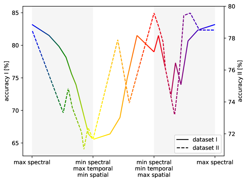
Figure 3: Accuracy along the triangle edges depicted in Figure 2. The colour of the curve allows to retrieve the feature resolution configuration from Figure 2. The curve has a large accuracy valley at maximal temporal information (yellow section), but also a smaller accuracy valley between the maximal spatial and spectral configuration (magenta section)

The method can be specifically applied for classification problems by adding the feature resolution parameters to the set of model hyperparameters. We hypothesise that the benefits of an optimal feature resolution configuration outweigh the costs incurred by the additional validation required.

References

- [1] B. Dubois, N. Villain, G. B. Frisoni, G. D. Rabinovici, M. Sabbagh, S. Cappa et al., “Clinical diagnosis of alzheimer’s disease: recommendations of the international working group,” The Lancet Neurology, vol. 20, no. 6, pp. 484–496, 2021.
- [2] J. Rasmussen and H. Langerman, “Alzheimer’s disease–why we need early diagnosis,” Degenerative neurological and neuromuscular disease, pp. 123–130, 2019.
- [3] G. Livingston, A. Sommerlad, V. Orgeta, C. Jack Jr, D. Bennett, K. Blennow et al., “Current and future treatments in alzheimer’s disease,” in Seminars in neurology, vol. 39, no. 02. Thieme Medical Publishers 333 Seventh Avenue, New York, NY 10001, USA., 2019, pp. 227–240.
- [4] P. M. Rossini, R. Di Iorio, F. Vecchio, M. Anfossi, C. Babiloni, M. Bozzali et al., “Early diagnosis of alzheimer’s disease: the role of biomarkers including advanced eeg signal analysis. report from the ifcn-sponsored panel of experts,” Clinical Neurophysiology, vol. 131, no. 6, pp. 1287–1310, 2020.
- [5] S. Goerttler, F. He, and M. Wu, “Understanding concepts in graph signal processing for neurophysiological signal analysis,” arXiv preprint arXiv:2312.03371, 2023.
- [6] D. Klepl, M. Wu, and F. He, “Graph neural network-based eeg classification: A survey,” arXiv preprint arXiv:2310.02152, 2023.
- [7] U. Von Luxburg, “A tutorial on spectral clustering,” Statistics and computing, vol. 17, pp. 395–416, 2007.
- [8] D. J. Blackburn, Y. Zhao, M. De Marco, S. M. Bell, F. He, H.-L. Wei et al., “A pilot study investigating a novel non-linear measure of eyes open versus eyes closed eeg synchronization in people with alzheimer’s disease and healthy controls,” Brain sciences, vol. 8, no. 7, p. 134, 2018.
- [9] A. Miltiadous, K. D. Tzimourta, T. Afrantou, P. Ioannidis, N. Grigoriadis, D. G. Tsalikakis et al., “A dataset of scalp eeg recordings of alzheimer’s disease, frontotemporal dementia and healthy subjects from routine eeg,” Data, vol. 8, no. 6, p. 95, 2023.
- [10] P. Welch, “The use of fast fourier transform for the estimation of power spectra: a method based on time averaging over short, modified periodograms,” IEEE Transactions on audio and electroacoustics, vol. 15, no. 2, pp. 70–73, 1967.