Engineering Hierarchical Symmetries

Abstract

We present a general driving protocol for many-body systems to generate a sequence of prethermal regimes, each exhibiting a lower symmetry than the preceding one. We provide an explicit construction of effective Hamiltonians exhibiting these symmetries. This imprints emergent quasi-conservation laws hierarchically, enabling us to engineer the respective symmetries and concomitant orders in nonequilibrium matter. We provide explicit examples, including spatiotemporal and topological phenomena, as well as a spin chain realizing the symmetry ladder $\text{SU(2)}{\rightarrow}\text{U(1)}{\rightarrow}\mathbb{Z}_{2}{\rightarrow}E$.

I Introduction

Symmetry is ubiquitous in nature, and it underpins intriguing and fundamental phenomena including the existence of conservation laws, integrability, the classification of phases of matter and transitions between them [1, 2], and it is a crucial component of a plethora of topological phenomena [3, 4]. Therefore, exploring protocols to engineer a desired symmetry and control its breaking, as well as investigating emergent phenomena associated with engineered symmetries, has attracted long-standing interest in both fundamental physics [5, 6, 7, 8, 9, 10, 11] and quantum engineering [12, 13, 14].

Recently, time-dependent protocols were proposed to Floquet-engineer symmetry as an emergent phenomenon [15, 16, 17, 18, 19, 20, 21], leading to the discovery of non-equilibrium phases of matter [22, 23, 24, 25, 26, 27, 28, 29, 30, 31]. However, little has been known about how to engineer sequences of different symmetries in a simple and controlled setting. This is a question of considerable importance for a variety of reasons. In statistical physics, symmetries can significantly impact how a system reaches thermal equilibrium [32, 33, 34, 35, 36, 37, 38]. Moreover, temporal sequences with specific symmetry content can be used to stabilize order in Floquet-engineered matter [39, 40]. They can also give rise to an interesting interplay of spontaneous with explicit symmetry breaking: from a practical perspective, engineered time-dependent symmetries can potentially enhance the control over wanted or unwanted spontaneous symmetry-breaking processes on real quantum devices [7, 41, 42, 43, 44, 45, 46, 47, 48].

In this work we study the engineering of hierarchical symmetries (HS) in a time-dependent set-up: we investigate whether or not, and under which conditions, a sequence of emergent symmetries can be engineered to occur hierarchically in time, in a controllable way. Realizing such HS in time-dependent systems is a demanding challenge, since: (1) A priori, explicit symmetry-breaking processes do not in general preserve any subgroup structure, and introduce transitions among all possible symmetry sectors; (2) Due to the absence of energy conservation in time-dependent systems, heating can further speed up the destruction of manifestations of symmetries, in particular quickly degrading any features sensitive to symmetry, e.g., melting any spontaneous-symmetry-breaking order.

Here, we propose a way to overcome these difficulties and construct a generic protocol to realize HS in driven many-body systems; it applies to any hierarchical symmetry group structure, irrespective of the specific microscopic details of the underlying model. It is explicit in that we provide a general scheme for realising any sequence of HS. In addition, this construction is not limited to Floquet systems, and also applies to more general time-dependence, e.g., quasi-periodically [49, 28, 50, 51, 52, 53, 54, 55], and even some randomly [56, 57], driven systems.

The key conceptual ingredient is a recursive time-dependent ansatz, in which unwanted processes, breaking a desired higher symmetry explicitly, cancel hierarchically in the high-frequency regime, cf. Fig. 1(a). Therefore, different symmetry-breaking effects only become noticeable beyond a sequence of long timescales. This leads to a corresponding sequence of prethermal steady-states with controllable lifetimes, each exhibiting a lower symmetry than the preceding one, cf. Fig 1(b) and (c) for an example. Our protocol thus also allows us to imprint emergent quasi-conservation laws hierarchically. Further, in conjunction with the process of spontaneous symmetry breaking, our scheme enables the engineering of different types of prethermal nonequilibrium order within the same time evolution.

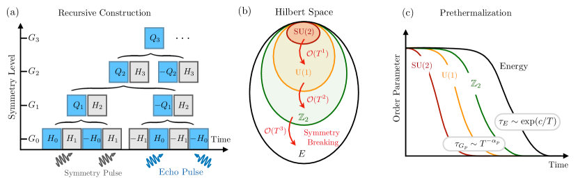
Figure 1: (a) Hierarchical symmetry breaking can be engineered via a recursive construction, where the “symmetry pulse” imposes a higher symmetry structure while the “echo pulse” cancels unwanted symmetry-breaking processes order by order. (b) Hilbert space showing a paradigmatic example of the symmetry ladder $\text{SU(2)}\rightarrow\text{U(1)}\rightarrow\mathbb{Z}_{2}\rightarrow E$, with $E$ denoting the trivial group. Symmetry breaking process can be parametrically suppressed by using a smaller driving period $T$. (c) Schematic for the sequence of prethermal steady states, exhibiting a lower symmetry than the preceding one. Their lifetimes scale algebraically with $T$ while heating in energy can be exponentially suppressed.

Our account is structured as follows. We first present a definition of hierarchical symmetry, and discuss its realization using nonequilibrium drives in Sec. II. This establishes the conceptual framework and as a result identifies the central ingredients of a pair of protocols, one of which is of operational simplicity and efficiency, while the other is of complete generality. In Sec. III we lay out an intuitive picture of our central result, illustrated by three explicit applications: (i) a spin chain with three engineered distinct prethermal steady-states, characterized by continuous non-Abelian SU(2), Abelian U(1), and discrete $\mathbb{Z}_{2}$ symmetry, respectively; (ii) a quantum clock model featuring a dynamical crossover between prethermal steady-states without equilibrium counterpart that exhibit $\mathbb{Z}_{4}$ and $\mathbb{Z}_{2}$ time crystalline order; and (iii) a free fermion system supporting a change in topology between a topological insulator (TI) and a higher-order topological insulator (HOTI) upon breaking time-reversal symmetry, as exemplified by the dynamical reduction of edge modes to corner/hinge modes in successive prethermal steady-states. We close with a summary of our results and an outlook with future applications in Sec. IV. Copious technical details are covered in supplemental materials.

II Implementing Hierarchical Symmetries

II.1 General recursive driving protocol

We first present our most fundamental result, namely an explicit general scheme for obtaining the HS for symmetry ladders as advertised above. We do this using the example of periodic drives, but the constructions proposed below are not limited to Floquet systems with step drives, and can also occur for continuous drives , and even quasi-periodically or randomly driven systems, as long as the dynamics can be approximated in a perturbative expansion by a sequence of effective Hamiltonian.

Consider a family of periodically driven systems, whose evolution operator over one period, $U_{F}$, is defined by concatenating $l$ (different) time evolution operators:

$$U_{F}=U_{l}U_{l-1}\cdots U_{1}\equiv e^{-iTQ}.$$ (1)

Whenever the drive frequency $\omega=2\pi/T$ is large compared to the typical local energy scales, periodically (and even randomly) driven systems exhibit a long-lived prethermal plateau [59, 60, 61, 28, 56] as a result of energy quasi-conservation. The dynamics can be approximated by a static effective Hamiltonian $Q_{[M]}$, obtained by means of the inverse-frequency expansion (IFE) [59]:

$$Q_{[M]}=\sum_{m=0}^{M}Q^{(m)},\qquad Q^{(m)}\propto T^{m},$$ (2)

with $M$ denoting the truncation order. Hence, generic ergodic systems evolve into a prethermal metastable state, described by the Generalized Canonical Ensemble, $\hat{\rho}_{\mathrm{GCE}}{\sim}{\exp{(-\sum_{\alpha}\lambda_{\alpha}C_{\alpha})}},$ with conserved quantities $C_{\alpha}$ associated with $Q_{[M]}$, and the Lagrange multipliers $\{\lambda_{\alpha}\}$ fixed by the initial state [33, 10]. We aim to construct a generic protocol that inscribes a structure of hierarchical symmetries into $Q_{[M]}$, one corresponding to each order $Q^{(m)}$ of the IFE. If we start from an ordered initial state that breaks the highest symmetry in $Q^{(0)}$, these symmetries will be revealed in the dynamics of the system via the occurrence of a hierarchical series of prethermal plateaus, cf. Fig 1(c).

Concretely, consider a finite set of Hamiltonian generators $H_{n},H_{n-1},\dots,H_{0}$ and an associated ladder of symmetry groups $G_{n}{\supset}G_{n-1}{\supset}{\cdots}{\supset}G_{0}$. Each Hamiltonian $H_{p}$ preserves the corresponding symmetry group $G_{p}$, so that $[H_{p},S_{q}]{=}0$ for all generators $S_{q}$ of $G_{q}$ with $q{\leq}p$; equivalently, each Hamiltonian $H_{p}$ breaks only one sub-symmetry of the symmetry ladder, reducing the symmetry group $G_{p+1}$ to $G_{p}$.

We realize such a symmetry hierarchy dynamically, by imprinting it iteratively in the structure of the effective Hamiltonian (2), order by order in the IFE. The Floquet unitary at (hierarchy) level-$n$ is constructed recursively as

$$U_{F,n} = e^{-il_{n-1}TQ_{n-1}}e^{-iTH_{n}}e^{+il_{n-1}TQ_{n-1}}e^{-iTH_{n}}$$ (3)

where $l_{n}{=}3{\times}2^{n}{-}2$ is the length of drive sequence, and we set $Q_{0}{=}H_{0}$, cf. Fig. 1(a). The effective stroboscopic generator at level-$n$ is defined via the relation, $U_{F,n}{\equiv}e^{-il_{n}TQ_{n}}$ . In A, we prove by induction that the corresponding IFE approximation at order $m$, $Q_{n}^{(m)}{\propto}T^{m}$ [cf. Eq. (2)], preserves the symmetry group $G_{n-m}$, $(n{-}m{\geq}0)$, and breaks explicitly all higher symmetries up the ladder. The key ingredient of this construction is that, in Eq. (3), the prefactors in front of the two $Q_{n-1}$ operators differ by a sign, ensuring the exact cancellation of $G_{n}$ symmetry-breaking terms in the leading order (time-average) $Q_{n}^{(0)}$.

II.2 Illustration of HS for small $n$

Let us explicitly illustrate the mechanism behind HS using a concrete example for small $n$. For $n{=}1$, we have

$$U_{F,1}{=}e^{-iH_{0}T}e^{-iH_{1}T}e^{iH_{0}T}e^{-iH_{1}T}.$$ (4)

The effective Hamiltonian to leading orders consists of $Q_{1}^{(0)}{\sim}H_{1}$ which preserves $G_{1}$, and $Q_{1}^{(1)}{\sim}T[H_{1},H_{0}]$ which reduces $G_{1}$ to $G_{0}$. Notice that the opposite signs in the prefactors in front of the two $H_{0}$ generators in the drive sequence ensure the exact cancellation of the $G_{1}$-breaking terms $H_{1}$ in the leading order $Q_{1}^{(0)}$; they only become effective at $\mathcal{O}(T)$ in $Q_{1}^{(1)}$.

At hierarchy level $n{=}2$, we introduce a new Hamiltonian $H_{2}$ which preserves $G_{2}$ (and hence also its subgroups $G_{1}$ and $G_{0}$). The new time evolution operator is $U_{F,2}{=}e^{-iQ_{1}l_{1}T}e^{-iH_{2}T}e^{iQ_{1}l_{1}T}e^{-iH_{2}T}.$ Now $Q_{2}^{(0)}{\sim}H_{2}$ preserves $G_{2}$, while $Q_{2}^{(1)}{\sim}T[H_{2},H_{1}]$ reduces $G_{2}$ to $G_{1}$; finally, $Q_{2}^{(2)}$ contains a term $T^{2}[H_{2},[H_{1},H_{0}]]$ which explicitly breaks $G_{1}$ to $G_{0}$. Note that, in practice, $e^{iQ_{1}l_{1}T}$ can be implemented by reversing the order of the temporal sequence of Eq. (4) and conjugating each individual driving element (i.e., going backward in time); this operation is generally accessible on current quantum computing platforms [31].

This construction can be performed recursively for higher $n$ and, remarkably, for each successive order of the IFE of the HS protocol in Eq. (3), $Q_{n}^{(m)}$ breaks only the corresponding successive subgroup, as desired. Note that we do not make any assumptions about the microscopic details of the generators $H_{n}$; hence, our construction is completely general and applies to any hierarchical symmetry group structure, making it widely applicable.

II.3 Sequence length, and shortening

Due to its recursive character, the generic driving sequence (3) is exponentially long, $l_{n}{\sim}2^{n}$, in the number $n$ of elementary unitary operators of the form $\exp(-icH_{k})$. Its appeal lies in its complete generality. Naturally, when considering applications to real physical systems (Sec. III), it is worthwhile to consider ways to shorten this sequence. Indeed, one can anticipate that the algebraic structure of the drive Hamiltonians may allow further contractions of the protocol.

As a concrete illustration of this possibility, consider three Hamiltonians $H_{2,1,0}$ corresponding to $G_{2}{\supset}G_{1}{\supset}G_{0}$; if, in addition, they obey the relation $[H_{0},H_{1}+H_{2}]{=}0$, then the shorter protocol

$$U_{F}{=}(e^{-iH_{0}T}e^{-iH_{1}T})e^{-iH_{2}T}(e^{iH_{0}T}e^{iH_{1}T})e^{-iH_{2}T}{=}e^{-iTQ}$$ (5)

defines an effective Hamiltonian, such that $Q_{2}^{(0)}{=}H_{2}$ has the symmetry group $G_{2}$, $Q_{2}^{(1)}$ reduces $G_{2}$ to $G_{1}$, and $Q_{2}^{(2)}$ breaks explicitly $G_{1}$ to $G_{0}$. A simple realization in spin-$1/2$ chains, discussed in C, corresponds to the symmetry ladder $\text{U(1)}{\rightarrow}\mathbb{Z}_{2}{\rightarrow}E$, with $E{=}\{id\}$ the trivial group. In the next section, we use this idea to implement an even more exotic four-step HS protocol featuring a non-abelian symmetry.

III Applications

In this section, we present applications of hierarchically engineered symmetries for three very different concepts/phenomena – non-Abelian symmetry, spatiotemporal order, and topological properties.

III.1 Implementation of Hierarchical Abelian and non-Abelian Symmetries

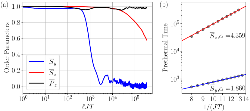
Figure 2: Dynamical detection of $\text{SU(2)}\rightarrow\text{U(1)}\rightarrow\mathbb{Z}_{2}\rightarrow E$ HS. (a) Dynamics of order parameters for the hierarchical quasi-conservation laws. Observables are normalized w.r.t. their initial values such that they all start from unity. Different lifetimes suggest that HS emerge at different time scales. (b) Lifetimes for each quasi-conservation law can be prolonged parametrically as $T^{-\alpha}$ in the high-frequency limit. The scaling exponent $\alpha$ follows the prediction by Fermi’s Golden Rule. We use $\delta_{x}/J{=}10,\epsilon/J{=}6$ and the coupling strength $J^{\prime}/J{=}5$. The numerical simulations are performed using exact diagonalization and $30$ random realizations of the driving protocol and initial state are used to compute the ensemble average.

We uncover the effects of HS via numerically simulating the dynamics of a paradigmatic many-body spin system with a rich emergent hierarchical symmetry structure $\text{SU(2)}{\rightarrow}\text{U(1)}{\rightarrow}\mathbb{Z}_{2}{\rightarrow}E$. To demonstrate that HS can occur beyond time-periodic systems, we consider a system driven by a fully random sequence built out of two possible unitaries $U_{\pm}$:

$$U_{\pm} \!\!\!=\!\!\! U(-H_{0}^{\pm},H_{1},H_{2},H_{0}^{\pm},-H_{1},H_{2},H_{3}|T/14){\times}$$

$$U(-H_{2},H_{1},-H_{0}^{\pm},-H_{2},-H_{1},H_{0}^{\pm},H_{3}|T/14),$$

where we define $U(D_{1},\dots,D_{l}|T){=}e^{-iD_{1}T}\cdots e^{-iD_{l}T}$ for simplicity, with many-body spin-${1}/{2}$ generators

$$H_{3}{=}J\sum_{\langle i,j\rangle}\sigma_{i}^{x}\sigma_{j}^{x}+\sigma_{i}^{y}\sigma_{j}^{y}+\sigma_{i}^{z}\sigma_{j}^{z},$$

$$H_{2}{=}J^{\prime}\sum_{\langle i,j\rangle}\sigma_{i}^{x}\sigma_{j}^{x}+\sigma_{i}^{y}\sigma_{j}^{y}-\sigma_{i}^{z}\sigma_{j}^{z},$$ (7)

$$H_{1}{=}-J^{\prime}\sum_{\langle i,j\rangle}\sigma_{i}^{y}\sigma_{j}^{y}-\sigma_{i}^{z}\sigma_{j}^{z},\;$$

$$H_{0}^{\pm}{=}(\delta_{x}\pm\epsilon)\sum_{i}\sigma_{i}^{x}.$$

The spins interact with their nearest neighbors with strength $J$ and $J^{\prime}$, and a uniform $x$-field of amplitude $\delta_{x}\pm\epsilon$ is applied randomly in time as the protocol sequence grows.

One can derive two different effective Hamiltonians $Q_{\pm}$ for $U_{\pm}$, which coincide up to the order $\mathcal{O}(T^{2})$, $Q_{+}^{(m)}{=}Q_{-}^{(m)}$ for $m{=}0,1,2$; this happens since, in the driving protocol, the only difference occurs through $H_{0}^{\pm}$, whose effect is suppressed to order $m\leq 2$ by the special construction Eq. (III.1). To leading order, summing up all generators, it is easy to see that $Q_{\pm}^{(0)}{\propto}H_{3}$ reproduces the Heisenberg model, preserving the highest symmetry SU(2); moreover, using IFE and the property $[H_{0}^{\pm},H_{1}{+}H_{2}]{=}0$, one can show that $Q_{\pm}^{(1)}=\mathcal{O}(T)$ reduces SU(2) to U(1); in turn, $Q_{\pm}^{(2)}=\mathcal{O}(T^{2})$ further reduces U(1) to a $\mathbb{Z}_{2}$ symmetry generated by the parity operator $P_{z}{=}\prod_{i}\sigma^{z}_{i}$ , cf. Fig 1(b) and C. This $\mathbb{Z}_{2}$ symmetry itself is weakly but explicitly broken by higher-order terms. Consequently, it is expected that, if we start from an SU(2)-broken initial state, the quasi-conservation laws associated with the above symmetries will persist with different lifetimes in the high-frequency (or small $T$) regime.

To verify this, we first prepare the initial state $|\psi(0)\rangle$ as a Haar random state in the $z$-magnetization block containing $N_{\downarrow}{=}6$ down spins out of all $L{=}16$ sites; it is then rotated around the $x$-axis by $\prod_{i}e^{-i\pi/16\sigma_{i}^{x}}$, resulting in an ordered state with non-zero initial magnetization along the $z$ and $y$ directions . If the SU(2) symmetry is preserved, both $S_{y}{=}\sum_{i}\sigma_{i}^{y}$ and $S_{z}{=}\sum_{i}\sigma_{i}^{z}$ are quasi-conserved quantities. As illustrated in Fig. 2a, for a fixed period $JT{=}0.1$, their normalized expectation values, $\bar{S}_{y/z}(t){=}\langle\psi(t)|S_{y/z}|\psi(t)\rangle/\langle\psi(0)|S_{y/z}|\psi(0)\rangle$, indeed remain almost unchanged until a long time scale $J\ell T\approx 5{\times}10^{2}$. Then, the system exhibits a noticeable decay in $\bar{S}_{x}$, indicating the explicit breaking of SU(2) by the higher-order terms in the IFE. By contrast, the quasi-conservation of $\bar{S}_{z}$ corresponding to the U(1) symmetry is more robust, and only exhibits roughly $20\%$ deviation from the initial unit value around $J\ell T{\approx}5{\times}10^{4}$, when the $y$-magnetization completely vanishes.

To detect the preservation of the $\mathbb{Z}_{2}$ symmetry, we measure the normalized expectation value of the parity operator $\bar{P}_{z}(t)$ which remains close to its initial value throughout the entire time evolution that we can numerically simulate.

The dynamics, constrained by all of these emergent symmetries, can be stabilized by using a higher drive frequency, and consequently, the lifetime of each quasi-conservation law can be parametrically prolonged. We define the lifetimes $\tau_{y}$ and $\tau_{z}$ as the time when the magnetizations $\langle S_{y}(t)\rangle$ and $\langle S_{z}(t)\rangle$ drop below the threshold values $e^{-1}$ and $e^{-0.45}$, respectively . As shown in Fig. 2b, in the high-frequency limit, both time scales follow an algebraic scaling in the form of $\tau\sim T^{-\alpha}$ with the scaling exponent $\alpha\approx 2$ for $\bar{S}_{y}$, and $\alpha\approx 4$ for $\bar{S}_{z}$, following the Fermi’s Golden Rule (FGR) prediction, cf. B. Since the $\mathbb{Z}_{2}$-breaking perturbations of $\mathcal{O}(T^{3})$ are extremely weak, it is challenging to determine the concrete scaling law for the lifetime of $\bar{P}_{z}$. In C, we consider another HS example to illustrate a simpler hierarchy $\text{U(1)}{\to}\mathbb{Z}_{2}{\to}E$, where we show that the decay of $\bar{P}_{z}$ can also be suppressed by using a shorter driving period. However, since $\bar{P}_{z}$ is a non-local operator, its decay may not be described by FGR.

HS stabilize quasi-conservation laws for both Abelian and non-Abelian, continuous and discrete symmetries with the corresponding timescales parametrically under control. In the following, we will go beyond and demonstrate how HS can be harnessed to engineer different types of non-equilibrium order, connected by dynamical crossover regimes and corresponding to the hierarchical symmetry groups, including spatiotemporal order (STO) and higher order topological insulating states.

III.2 Hierarchical Symmetry Reduction in a
$\mathbb{Z}_{4}$ Discrete Time Crystal

We begin with STO and consider a 4-state clock model, whose kicked dynamics is generated by

$$H_{0} = \sum_{i=1}^{L}b_{i}(Z_{i}+Z_{i}^{\dagger})$$

$$H_{1} = \sum_{\langle i,j\rangle}J_{ij}\left(Z_{i}^{2}Z_{j}^{2}-\eta(e^{i\phi}Z_{i}^{\dagger}Z_{j}+\text{h.c.})\right)$$

$$+\sum_{i}h_{i}\left(Z_{i}^{2}-\frac{1}{2}\left(X_{i}+X_{i}^{\dagger}\right)\right)+\sum_{i}g_{i}X_{i}^{2},$$

where $J_{ij}$ is a nearest neighbor interaction strength, $g_{i}$ an onsite $X^{2}$ interaction, and $b_{i}$ is a parallel field; $h_{i}$ measures the strength of a combination of the onsite $Z^{2}$-interaction and the transverse field; $\eta$ and $\phi$ help stabilize the STO [66]. We introduce randomness in the form of uniformly distributed spatial disorder in all couplings, to reduce finite-size effects that manifest as temporal fluctuations in the dynamics of observables. In the $Z$-eigenbasis denoted by $|n\rangle$, $n=0,1,2,3$,

$$Z=\begin{pmatrix}1&0&0&0\\ 0&-i&0&0\\ 0&0&-1&0\\ 0&0&0&i\end{pmatrix},\quad X=\begin{pmatrix}0&1&0&0\\ 0&0&1&0\\ 0&0&0&1\\ 1&0&0&0\end{pmatrix},$$ (9)

satisfy the commutation relations $Z_{j}X_{k}{=}e^{\frac{i\pi}{2}\delta_{jk}}X_{k}Z_{j}$, and $X_{j}^{4}{=}1{=}Z_{j}^{4}$. The $X$ operator shifts the population of the four $|n\rangle$ states cyclically. Hence, the internal level structure admits a $\mathbb{Z}_{4}$ symmetry. This symmetry is obeyed by the nearest-neighbor interaction and the $X^{2}$ terms, and broken down to a $\mathbb{Z}_{2}$ subgroup by the $Z^{2}$ on-site term; the parallel field further reduces this remaining symmetry to the trivial group, $\mathbb{Z}_{2}\to E$.

When the kicked dynamics of the system, generated by $H_{0}$ and $H_{1}$, is interleaved with $T$-periodic $X$-kicks, $P_{X}=\prod_{i}X_{i}$,

$$U_{F} = e^{iH_{0}T/4}e^{-iH_{1}T/4}e^{-iH_{0}T/4}e^{-iH_{1}T/4}P_{X},$$ (10)

the $\mathbb{Z}_{4}$ symmetry can conspire with the discrete time-translation symmetry and induce spatiotemporal order, much like in a $\mathbb{Z}_{4}$-time crystal [66]. The kick generators $H_{0}$, $H_{1}$ are designed to imprint HS in the first few orders of the effective Hamiltonian associated with Eq. (10). In particular, using the relation $\sum_{q=0}^{3}[X^{q}]^{\dagger}Z^{p}X^{q}{=}0$ ($p{\in}\mathbb{N}$), one can show that the leading-order term $Q^{(0)}$ has a $\mathbb{Z}_{4}$ symmetry which gets reduced to its $\mathbb{Z}_{2}$ subgroup by $Q^{(1)}$, while higher-order terms possess no symmetry; the explicit form of the effective Hamiltonian is given in D. As a result, the system exhibits two prethermal STO states within its time evolution (one for each emergent symmetry in the ladder), connected by a smooth crossover in time and stabilized by disorder.

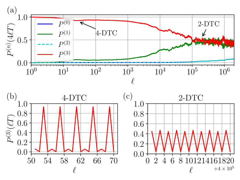
Figure 3: $\mathbb{Z}_{4}$ quantum clock model. Time evolution of average population $P^{(n)}(t_{\ell}){=}L^{-1}\sum_{j=1}^{L}\langle\psi(t_{\ell})|p_{j}^{(n)}|\psi(t_{\ell})\rangle$ in the clock state $|n\rangle$ at $t_{\ell}=4\ell T$, starting from the initial state $\left|\psi(0)\right\rangle{=}\left|3\right\rangle^{\otimes L}$ and being averaged over 50 realizations. (a) Population $P^{(n)}(t_{\ell})$ at $t_{\ell}=4\ell T$ and the dynamic crossover between two spatial-temporal orders. (b) $Z_{4}$ plateau, system oscillates between these four local state and their superposition which is a 4-DTC behaviour. (c) $\mathbb{Z}_{2}$ plateau, the odd and even local states merge in pairs (dash line), and system finally exhibit 2-DTC behavior. The parameters are $T=0.5$, $\eta{=}0.35$, $\phi{=}\pi/3$, and $J_{ij}\in(0.5,1.5)$, $g_{i}\in(0,0.3)$, $h_{i}\in(0,0.6)$, $b_{i}\in(0,2.5)$ are drawn from a uniform distribution in the given interval.

Figure 3a shows the dynamics of the population $p^{(n)}{=}|n\rangle\langle n|$ of each of the four clock states $|n\rangle$ at times $t_{\ell}{=}4\ell T$, averaged over the lattice, starting from the initial product state $\left|\psi(0)\right\rangle{=}\left|3\right\rangle^{\otimes L}$. Two prethermal plateaus, corresponding to $\mathbb{Z}_{4}$ and $\mathbb{Z}_{2}$ quasi-conservation, are clearly visible in Fig. 3a. Their lifetime can be increased by decreasing the drive period $T$. In the $\mathbb{Z}_{4}$-plateau governed by $Q^{(0)}$, the population exhibits period-4 oscillations in time [Fig. 3b], characteristic of prethermal 4-DTC order. As time progresses, $Q^{(1)}$ asserts itself, and hence the dynamics crosses over to the $\mathbb{Z}_{2}$-plateau. The explicit breakdown of the original $\mathbb{Z}_{4}$-symmetry causes the population to redistribute, while subject to the surviving $\mathbb{Z}_{2}$-quasiconstraint. As a result, akin to prethermal 2-DTC order, the population keeps oscillating between two states [Fig. 3c], described by a statistical mixture of the bare even/odd clock states that halves the oscillation amplitude. Hence, the manifestation of this spatiotemporal HS ladder is reflected in the change of the characteristic periodic signature of observable expectations as a function of time. Due to the ultimate breakdown of the $\mathbb{Z}_{2}$ symmetry by the higher-order effective Hamiltonians $Q^{(m\geq 2)}$, the population gradually spreads over all clock states, as evidenced by the rise of the blue and cyan curves in Fig. 3a. Eventually, at even longer times the final state of the system is evenly distributed among the four clock states, corresponding to a featureless infinite-temperature state [not shown].

III.3 High-order Topological Insulators from
Hierarchical Symmetries

Symmetries play a fundamental role also in topological quantum matter; this is perhaps most prominently encoded in the notion of symmetry-protected topological phases (SPTs), where topological stability is predicated on the presence of a particular symmetry [3, 4]. We now demonstrate how HS can change the topological character of, say, electronic systems by altering the underlying symmetry. We start from a topological insulator (TI) in a 2D lattice, protected by time reversal symmetry $\mathcal{T}$ and crystalline inversion symmetry $\mathcal{I}$. Subject to open boundary conditions, the single-particle spectrum of the Hamiltonian $H_{\text{TI}}$ exhibits topological edge modes. In such materials, an initial state with significant support on the edge of a sample will keep this support during the time evolution generated by $H_{\text{TI}}.$ Perturbations that break time reversal $\mathcal{T}$ but preserve inversion symmetry $\mathcal{I}$ cause a topological phase transition from a TI to a higher-order topological insulator (HOTI) [67]. The characteristic feature of HOTI is the presence of corner states whose support is localized only at the corners of the sample, reflecting the reduced symmetry group.

A change of topology from a TI to a HOTI can naturally be exhibited by the transient dynamics of Floquet systems that realize the HS ladder $\mathcal{T}{\times}\mathcal{I}{\rightarrow}\mathcal{I}{\rightarrow}E$. Intuitively, initial states with weight concentrated on the edge modes will remain stable over a controllable timescale, before the leading-order symmetry-reducing term takes over; then only modes supported on the corners survive, while other edge modes start delocalizing into the bulk as a result of broken time reversal. Eventually, if present, interactions will cause the system to heat up to an infinite temperature state and lose all nontrivial topological properties.

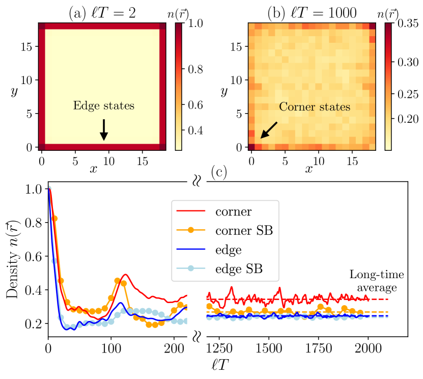
Figure 4: Topological corner states stabilized by HS. Time evolution of the electron density on site $\vec{r}=(x,y)$, $n({\vec{r}}){=}\sum_{\sigma=\uparrow,\downarrow}\sum_{q=0,1}\left\langle c_{\sigma,q}^{\dagger}(\vec{r})c_{\sigma,q}(\vec{r})\right\rangle$, starting from the initial state that fully cover the edge. (a-b) Snapshots of the density distribution show a dynamical change of topology, manifest in a transition from an edge state (TI) to a corner state (HOTI). (c) Dynamics of the density at the corner (red line) $n_{\text{corner}}=(n{(0,0)}+n{(L,L)})/2$ and the edge (blue line) $n_{\text{edge}}=2\sum_{i=L/4}^{3L/4}n{(i,0)}/L$ using a HS ladder. If the first-order perturbation explicitly breaks $\mathcal{I}$, support on the corner becomes less dominant (orange) while the edge maintains approximately the same density at long times (dashed lines). We use $M=1.0,J=1.0,\Delta_{0}=1.0,\Delta_{1}=7.0,\Delta_{2}=12.0$ and $T=0.2$ for numerical simulation.

To demonstrate this explicitly, we consider the Floquet unitary

$$U_{F} \!\!\!=\!\!\! U\left(H_{0},\frac{H_{1}}{2},\frac{H_{1}^{\prime}}{2},-H_{0},\frac{H_{1}}{2},\frac{H_{1}^{\prime}}{2},H_{2}\bigg{|}\frac{T}{10}\right){\times}$$

$$U\left(-\frac{H_{1}}{2},-\frac{H_{1}^{\prime}}{2},H_{0},-\frac{H_{1}}{2},-\frac{H_{1}^{\prime}}{2},-H_{0},H_{2}\bigg{|}\frac{T}{10}\right)$$

for a set of four 4-band Hamiltonians $H_{0,1,2}^{(^{\prime})}$ on a 2D square lattice, involving two orbital angular momentum and two spin degrees of freedom, described by the Pauli matrices $\tau$ and $\sigma$, respectively. Going to momentum space using $H_{j}{=}\sum_{\vec{k}}\psi_{\vec{k}}^{\dagger}H_{j}(\vec{k})\psi_{\vec{k}}$ with $\psi_{\vec{k}}{=}[c_{\uparrow,0}(\vec{k}),c_{\downarrow,0}(\vec{k}),c_{\uparrow,1}(\vec{k}),c_{\downarrow,1}(\vec{k})]$, we have

$$H_{2}(\vec{k}) = \left[M+J(\cos k_{x}+\cos k_{y})\right]\;\tau_{z}\sigma_{0}$$

$$H_{1}(\vec{k}) = \Delta_{1}\tau_{z}(\sigma_{x}+\sigma_{y}),$$

$$H_{1}^{\prime}(\vec{k}) = \Delta_{1}\tau_{z}\sigma_{z},$$

$$H_{0}(\vec{k}) = \Delta_{2}\tau_{x}\sigma_{y}.$$ (12)

The representation of the Hamiltonian in real space is shown in D. Compared to Eq. (3), Eq. (III.3) features additionally $H_{1}^{\prime}$ which introduces an onsite $\mathcal{T}$ breaking term in the effective Hamiltonian that opens up the energy gap at the band touching point of $H_{2}$ to produce the HOTI.

The time-reversal symmetry can be represented as $\mathcal{T}{=}i\tau_{0}\sigma_{y}K$, with $K$ the complex conjugation, and acts on the Hamiltonian (III.3) by $\vec{k}{\to}{-}\vec{k}$ and $\mathcal{T}\vec{\sigma}\mathcal{T}^{-1}{=}{-}\vec{\sigma}$; inversion symmetry $\mathcal{I}{=}\tau_{z}\sigma_{0}$ transforms $\vec{k}{\to}{-}\vec{k}$ and $\mathcal{I}\tau_{x,y}\mathcal{I}^{-1}{=}{-}\tau_{x,y}$. Therefore, $H_{2}$ is invariant under both $\mathcal{I}$ and $\mathcal{T}$, and hosts the well-known $\mathbb{Z}_{2}$-TI for $|M|{<}2|J|$. As a consequence, the leading order effective Hamiltonian $Q^{(0)}{\propto}H_{2}$ inherits the topological property of $H_{2}$. Moreover, note that the terms proportional to $\Delta_{1}$ break $\mathcal{T}$, while the $\Delta_{2}$ term breaks both $\mathcal{T}$ and $\mathcal{I}$; therefore, $Q^{(1)}{\propto}\tau_{0}(\sigma_{x}-\sigma_{y})$ breaks $\mathcal{T}$ but preserves $\mathcal{I}$. This allows the protocol in Eq. (III.3) to induce a dynamical crossover in topological order from TI to HOTI. The complete effective Hamiltonian and its eigenvalue spectrum can be found in D.

To exhibit this topological HS ladder, we prepare the initial state as the product state in the real-space Fock basis to fully cover the edge of the 2D lattice; on each edge site the same internal degree of freedom $(\downarrow,1)$ is occupied, i.e., $\left|\psi_{0}\right\rangle{=}\prod_{\vec{r}\in\text{edge}}{c}^{\dagger}_{\downarrow,1}(\vec{r})\left|0\right\rangle$. Since this initial state has a large overlap with the localized edge state of $Q^{(0)}$, the initial configuration remains almost unchanged at the early evolution times, as shown by the real-space density $n(\vec{r})$ at time $\ell T=2$ in Fig. 8a. The persistence of the edge density can be more pronounced if we initialize the system in one of the localized eigenstates of $Q^{(0)}$, cf. E.

At later times, the system starts delocalizing into the bulk but the occupation around the corners persists, cf. Fig. 8b, due to the surviving inversion symmetry in $Q^{(1)}$, which is required for the HOTI [in our model, the zero-energy corner state occupies only two of the four corners]. We also depict the density at the corner (red line) and the edge (blue line) in panel Fig. 8c; clearly, the corner density has larger support especially at long times (dashed lines).

To highlight the importance of using HS in stabilizing the corner state, we also plot the dynamics (dotted lines) with different Hamiltonians $H_{1}{=}\Delta_{1}\tau_{x}(\sigma_{x}+\sigma_{y})$, $H_{1}^{\prime}{=}\Delta_{1}\tau_{0}\sigma_{z}$, such that the first order IFE correction explicitly breaks all symmetries at once. As shown in panel Fig. 8c, in this case, the support on the corner state (dotted orange) stabilizes at twice a smaller value compared to the HS case . By contrast, the edge density (light blue) remains approximately unchanged at long times.

IV Discussion and Outlook

We present a constructive framework to engineer symmetry reduction hierarchically in driven many-body systems via a recursive time-dependent ansatz. This permits us to impose hierarchical quasi-conservation laws and to realize various kinds of order in nonequilibrium matter. The lifetime of such ordered states accessible via HS, is parametrically controllable and can be obtained using Fermi’s Golden rule, see B.

We demonstrate HS in systems with different global symmetries, inducing dynamical crossovers between both equilibrium and nonequilibrium ordered states, including topological states. The generalization to local gauge symmetries presents an interesting open direction [69]: e.g., in the Floquet-engineered Kitaev honeycomb model [19, 20, 21] HS can play an important role in stabilizing exotic fractionalized phases of matter. HS also have the potential to significantly suppress errors in the quantum simulation of time-dependent systems thereby improving the robustness of quantum algorithms whenever symmetry plays a central role as in, e.g., quantum error correction [70, 71, 72].

HS constructions apply equally to fermionic and bosonic, interacting and noninteracting quantum models that exhibit hierarchical symmetries and are, therefore, widely accessible in various experimental platforms. For example, the Heisenberg model with tunable anisotropy in Eq. (III.1) has already been realized in cold atoms systems and superconducting qubits [73, 14, 74, 47]. HS can be readily implemented in the lab since the underlying echo-out mechanism generalizes state-of-the-art dynamical decoupling techniques [44]; they can also be used to achieve enhanced control over higher-order corrections. Particularly intriguing is the possibility of experimentally studying the properties of distinct ordered states within different prethermal stages of the same time evolution.

On a fundamental level, spontaneous symmetry breaking (SSB) of approximate (i.e., weakly explicitly broken) continuous symmetries gives rise to weakly gapped Goldstone modes [75]. These gapped excitations will naturally appear during the hierarchical symmetry breaking of $\text{SU(2)}{\rightarrow}\text{U(1)}{\rightarrow}\mathbb{Z}_{2}{\rightarrow}E$, provided that the system is initialized at low-enough temperatures. A systematic investigation of this phenomenon would provide valuable insights on SSB in driven systems, opening up new avenues for future work.

We emphasize that discussions regarding engineered symmetry breaking are not limited to quantum or Hamiltonian systems. It is intriguing to generalize the analysis of the symmetry structure to Liouvillians [76, 77, 78, 79], and we anticipate applications of HS in time-dependent open quantum systems and classical many-body setups. In particular, numerical simulation of classical systems is not limited to small system sizes and hence novel prethermal phases in higher dimensions induced by HS can be explored [80, 81, 82, 83, 84]. Understanding the richer hierarchical structure of weak and strong symmetries in open systems is an open avenue for future studies [85, 71]. Moreover, generalizing the current framework to engineer integrability breaking  [86] and to control classical chaos would be worthwhile to pursue.

Finally, our work also raises the intriguing converse question of whether or not one can design protocols that systematically enlarge a given symmetry group.

Acknowledgments.—We thank A. Dymarsky, M. Heyl, F. Pollmann, F. Schindler and Y. Hou for enlightening discussions. This work is in part supported by the Deutsche Forschungsgemeinschaft under cluster of excellence ct.qmat (EXC 2147, project-id 390858490). Funded by the European Union (ERC, QuSimCtrl, 101113633). Views and opinions expressed are however those of the authors only and do not necessarily reflect those of the European Union or the European Research Council Executive Agency. Neither the European Union nor the granting authority can be held responsible for them. This research was supported in part by the International Centre for Theoretical Sciences (ICTS) for participating in the program - Stability of Quantum Matter in and out of Equilibrium at Various Scales (code: ICTS/SQMVS2024/01)

Appendix A General Protocol for Arbitrary Order of HS

A.1 General Driving Protocol: Iterative Proof

In this section, we prove that the recursive time-dependent construction in Eq. (3), introduced in the main text, can realize hierarchically the symmetries of the symmetry ladder

$$G_{n}\supset G_{n-1}\supset G_{n-2}\supset\cdots\supset G_{1}\supset G_{0}.$$ (13)

We illustrate the basic idea with a simple and concrete example before discussing the general proof.

Consider a Hamiltonian $H_{1}$ which preserves the symmetry $G_{1}$ and a Hamiltonian $H_{0}$ which only preserves a subgroup $G_{0}$ of $G_{1}$, i.e., $G_{1}\supset G_{0}$. We construct the following Floquet operator

$$U_{1}\equiv e^{-iQ_{1}l_{1}T}=e^{-iH_{0}T}e^{-iH_{1}T}e^{iH_{0}T}e^{-iH_{1}T},$$ (14)

where $l_{n}\equiv-2+3\times 2^{n}$. The effective Hamiltonian reads $Q_{1}=Q_{1}^{(0)}+Q_{1}^{(1)}+\mathcal{O}(T^{2})$, with $Q_{1}^{(0)}\sim H_{1}$ preserving $G_{1}$ and, $Q_{1}^{(1)}\sim T[H_{1},H_{0}]$ reducing $G_{1}$ to $G_{0}$. Notice that in Eq. (14) the prefactors in front of the two $H_{0}$ operators differ by a sign, ensuring the exact cancellation of $H_{1}$ symmetry-reducing terms in the leading order (time-average) $Q_{1}^{(0)}$. This mechanism is the key ingredient for the proposed recursive construction.

Now we go one step further by introducing yet a new Hamiltonian $H_{2}$ which preserves the symmetry $G_{2}$, such that $G_{2}\supset G_{1}\supset G_{0}$. Therefore, $H_{2}$ also preserves $G_{1}$ and $G_{0}$ by construction. The new time evolution operator is

$$U_{2}\equiv e^{-iQ_{2}l_{2}T}=e^{-iQ_{1}l_{1}T}e^{-iH_{2}T}e^{iQ_{1}l_{1}T}e^{-iH_{2}T},$$ (15)

where $Q_{2}=Q_{2}^{(0)}+Q_{2}^{(1)}+Q_{2}^{(2)}+\mathcal{O}(T^{3})$. Similar to the case above, the prefactors in front of $Q_{1}$ differ by a sign, and one can verify that $Q_{2}^{(0)}\sim H_{2}$ preserves $G_{2}$, $Q_{2}^{(1)}\sim T[H_{2},Q_{1}^{(0)}]\sim T[H_{2},H_{1}]$ reduces $G_{2}$ to $G_{1}$. Finally, $Q_{2}^{(2)}\sim T^{2}(\alpha_{1}[H_{2},Q_{1}^{(1)}]+\alpha_{2}[H_{2},[H_{2},Q_{1}^{(0)}]+\alpha_{3}[Q_{1}^{(0)},[Q_{1}^{(0)},H_{2}]])$ for some coefficients $\alpha_{i}$ and, importantly, the term with prefactor $\alpha_{1}$ reduces $G_{1}$ to $G_{0}$ since $Q_{1}^{(1)}$ does so alone. In general, it follows that the $m$-th order term $Q_{2}^{(m)}$ contains at most the $(m-1)$-th order term $Q_{1}^{(m-1)}$ from the IFE expansion of $Q_{1}$.

These basic observations suggest that if we iteratively construct a new evolution operator $U_{n}$, the previous HS structure can be embedded into the effective Hamiltonian of $U_{n}$, while the zeroth-order of the effective Hamiltonian is proportional to the newly added Hamiltonian which obeys the highest symmetry group. In addition, the structure of level $(n-1)$ HS ladder is embedded in the level $n$ HS ladder. In practice, $e^{iQ_{1}l_{1}T}$ can be implemented by reversing the order of the temporal sequence of Eq. (14) and conjugating each individual driving element (i.e., going backward in time).

We can now give a more general construction and its proof based on induction. Consider a set of Hamiltonian $\{H_{r}\}$ with a symmetry ladder $\{G_{r}\}$ and corresponding symmetry generators $\{S_{r}\}$:

$$H_{n-1},H_{n-2},\cdots,H_{1},H_{0};$$ (16)

$$G_{n-1}\supset G_{n-2}\supset\cdots\supset G_{1}\supset G_{0};$$

$$[H_{p},S_{q}]=0,\forall q\leq p.$$

Let us assume that the $(n-1)$-th order time-evolution operator $U_{n-1}=e^{-iQ_{n-1}l_{n-1}T}$ has the following property

$$Q_{n-1}=\sum_{m}Q_{n-1}^{(m)},$$ (17)

$$[Q_{n-1}^{(m)},S_{q}]=0,\forall q<n-m-1,\qquad[Q_{n-1}^{(m)},S_{q}]\neq 0,\forall q\geq n-m-1,$$

such that $U_{n-1}$ already implements the above level-$(n-1)$ HS.

Next we add a new Hamiltonian $H_{n}$ which obeys a higher symmetry $G_{n}$,

$$[H_{n},S_{n}]=0,G_{n}\supset G_{n-1},$$ (18)

and extend the drive protocol to

$$U_{n}=e^{-iQ_{n-1}l_{n-1}T}e^{-iH_{n}T}e^{iQ_{n-1}l_{n-1}T}e^{-iH_{n}T}\equiv e^{-iQ_{n}l_{n}T}.$$ (19)

Again, the prefactors in front of two $Q_{n-1}$ differ by a sign. One can check that, for $n=1$, we recover Eq. (14).

Using the Baker-Campbell-Hausdorff (BCH) expansion, we get the perturbative expansion of $Q_{n}$ as a power series of $T$

$$Q_{n}=\frac{2}{l_{n}}H_{n}+\lambda_{1}T[H_{n},Q_{n-1}]+\lambda_{2}T^{2}([H_{n},[H_{n},Q_{n-1}]]+l_{n-1}[Q_{n-1},[Q_{n-1},H_{n}]])+\cdots,$$ (20)

$$\lambda_{1}=i\frac{l_{n-1}}{l_{n}},\lambda_{2}=-\frac{l_{n-1}}{2l_{n}}.$$

Observe that the leading order term preserves $G_{n}$; the strength of the $G_{n-1}$-reducing term is renormalized by an extra factor of $T$; the strength of the $G_{n-2}$-reducing term is renormalized by the extra factor $T^{2}$, etc. More precisely, the $\mathcal{O}(T^{m})$ term in BCH expansion of $Q_{n}$ takes the following form

$$Q_{n}^{(m)}=\sum_{p=1}^{m}f_{p}(Q_{n-1}^{(m-p),(m-p-1),\cdots,0}),$$ (21)

where $f_{p}(Q_{n-1}^{(m-p),(m-p-1),\cdots,0})$ involves nested commutators of $H_{n}$ and $Q_{n-1}^{(m-p)},Q_{n-1}^{(m-p-1)},\cdots,Q_{n-1}^{0}$; for example, $f_{1}(Q_{n-1}^{(m-1)})=\lambda_{1}T[H_{n},Q_{n-1}^{(m-1)}]$. Since the Hamiltonian with the highest order of $T$ in $f_{p}(Q_{n-1}^{(m-p),(m-p-1),\cdots,0})$ is $Q_{n-1}^{(m-p)}$, which explicitly breaks the symmetry group $G_{n-1-(m-p)}$ but preserves all lower-order symmetries $G_{q}$, we have

$$[f_{p}(Q_{n-1}^{(m-p),\cdots}),S_{q}]=0,\qquad\forall q<n-1-m+p.$$ (22)

Therefore, for $Q^{(m)}_{n}$, the first symmetry group along the ladder which is explicitly broken is $G_{n-m}$, i.e.,

$$[Q_{n}^{(l)},S_{q}]=0,\qquad\forall q<n-m.$$ (23)

Note that the conditions in Eq. (LABEL:Eq.induction) are now generalized to $Q_{n}$, which completes the induction step. The new symmetry ladder is Eq. (13), as desired.

A.2 Implementing symmetry-breaking at arbitrary-order of the inverse-frequency expansion

The HS structure is not necessary to have the perturbations aligned order by order in the effective Hamiltonian. We can make symmetry-breaking terms appear in an arbitrarily high-order term using our proposed protocol. The proof is very intuitive: assuming that we already have the evolution operator $U_{n-1}\equiv e^{-i\ell_{n-1}Q_{n-1}T}=e^{-i\ell_{n-2}Q_{n-2}T}e^{-iH_{n-1}T}e^{i\ell_{n-2}Q_{n-2}T}e^{-iH_{n-1}T}$ with HS structure, we know that normally $Q_{n-1}^{(1)}$ breaks $G_{n-1}$. However, if we impose that the newly introduced Hamiltonian $H_{n}$ in the protocol preserves the symmetry $G_{n-1}$ rather than $G_{n}$, it is clear that $Q_{n}^{(0)}$ and $Q_{n}^{(1)}$ will both preserve $G_{n-1}$, while the $G_{n-1}$-breaking term will become a higher-order perturbation.

One of the simplest ways to engineer this is to choose $H_{n}=H_{n-1}$; the evolution operator in this case is

$$U_{n}\equiv e^{-i\ell_{n}Q_{n}T}=(e^{-i\ell_{n-2}Q_{n-2}T}e^{-iH_{n-1}T}e^{i\ell_{n-2}Q_{n-2}T})e^{-iH_{n-1}T}(e^{-i\ell_{n-2}Q_{n-2}T}e^{iH_{n-1}T}e^{i\ell_{n-2}Q_{n-2}T})e^{-iH_{n-1}T}.$$ (24)

Repeating this operation we can push the symmetry-breaking term to an arbitrarily high order. Moreover, this observation holds for any symmetry in the symmetry ladder.

A.3 Shortening the HS drive sequence

The general construction shown in Sec. A.1 is exponentially long in $n$. Here, we illustrate the possibility of using additional properties of the generating Hamiltonians to shorten the drive sequence. Consider the example Eq. (5) discussed in the main text

$$U_{2}=(e^{-iH_{0}T}e^{-iH_{1}T}e^{-iH_{2}T})(e^{iH_{0}T}e^{iH_{1}T}e^{-iH_{2}T}),$$ (25)

using the property $[H_{0},H_{1}+H_{2}]=0$ we can achieve level-2 HS with a shorter driving sequence (compared to the general construction presented in Sec. A). For level-3 HS, an option for reducing the drive sequence is using $U_{2}$ above and define $U_{3}=U_{2}e^{-iH_{3}T}U_{2}^{\dagger}e^{-iH_{3}T}$ without imposing any extra limitations on $H_{3}$, as the SU(2) case in the main text(length of the driving sequence $\ell=14$).

Another way is to impose a condition on the structure of the newly added Hamiltonian $H_{3}$: consider the evolution operator

$$U_{3}\equiv e^{-i8Q_{3}T}=(e^{-iH_{0}T}e^{-iH_{1}T}e^{-iH_{2}T}e^{-iH_{3}T})(e^{iH_{1}T}e^{iH_{2}T}e^{iH_{0}T}e^{-iH_{3}T}).$$ (26)

The first three orders of $Q_{3}$ are

$$Q_{3}^{(0)} \sim H_{3}$$

$$Q_{3}^{(1)} \sim iT([H_{3},H_{2}]+[H_{3}+H_{2},H_{1}]+[H_{3},H_{0}])$$

$$Q_{3}^{(2)} \sim T^{2}(Q_{1,2,3}+[H_{0},[H_{0},H_{3}]]-[H_{3},[H_{0},H_{3}]]+2[H_{0},([H_{1},H_{2}+H_{3}]+[H_{2},H_{3}])]),$$ (27)

where $Q_{1,2,3}$ is a short-hand notation for the effective Hamiltonian that contains only commutators of $H_{1}$, $H_{2}$, and $H_{3}$. In order to achieve HS structure, the terms containing $H_{1}$ and $H_{0}$ should vanish in $Q_{3}^{(1)}$ and terms containing $H_{0}$ should vanish in $Q_{3}^{(2)}$. Therefore, one of the simplest conditions one can impose is

$$[H_{0},H_{3}]=0,\qquad[H_{0},H_{2}]=0,\qquad[H_{1},H_{2}+H_{3}]=0.$$ (28)

These special cases can be used as building blocks for longer symmetry ladders. For even higher-level HS, a driving sequence can be constructed based on the above two special cases by the previous iterative method to reduce the sequence length. Whether there exists further shortening of the pair of driving sequences with pragmatically meaningful conditions on the Hamiltonians for higher-level HS, remains an open question.

A.4 Generalizations of the hierarchical symmetry protocols

In this section, we will discuss two more generalizations of the protocol we proposed before, which enable us to manipulate the effective Hamiltonian in a different way. The first one generalizes the single Hamiltonian $H_{n}$ to an effective Hamiltonian $P_{n}$ from the symmetry-preserving driving sequence. This has important implications for the realization of HS on real quantum devices because sometimes, instead of directly simulating $H_{n}$, one may approximate its time evolution via Trotterization. One example is the 1D Heisenberg model, whose time evolution can be Trotterized into even and odd-bond updates, both of which satisfy the desired SU(2) symmetry [46]. The second one allows us to embed specific terms in the effective Hamiltonian to tailor its properties. As we will discuss in the following, we use this method to open the energy gap in the topological example, which generates a corner state.

Generalization 1. Considering the following evolution operator

$$U_{n}\equiv e^{-iQ_{n}l_{n}T}=e^{-iQ_{n-1}l_{n-1}T}e^{-iP_{n}T}e^{iQ_{n-1}l_{n-1}T}e^{-iP_{n}^{\prime}T},$$ (29)

$$e^{-iP_{n}T}\equiv\prod_{i=1}^{p_{n}}e^{-iH_{n,i}T/p_{n}},\qquad e^{-iP_{n}^{\prime}T}\equiv\prod_{i=1}^{p_{n}^{\prime}}e^{-iH_{n,i}^{\prime}T/p_{n}^{\prime}},$$ (30)

where $P_{n}$ and $P_{n}^{\prime}$ are defined as the effective Hamiltonian of the driving sequence defined in Eq. (30) and $H_{n,i}$, $H_{n,i}^{\prime}$ all preserve the symmetry $G_{n}$. The effective Hamiltonian reads

$$Q_{n} = \frac{1}{\ell_{n}}(P_{n}+P_{n}^{\prime})+\frac{iT}{\ell_{n}}\left(\ell_{n-1}[P_{n},Q_{n-1}]+\frac{1}{2}[P_{n}^{\prime},P_{n}]\right)$$ (31)

$$-\frac{T^{2}}{12\ell_{n}}\left(6\ell_{n-1}^{2}[Q_{n-1},[Q_{n-1},P_{n}]]+6\ell_{n-1}[P_{n}^{\prime},[P_{n},Q_{n-1}]]+[P_{n}-P_{n}^{\prime},[P_{n},P_{n}^{\prime}]]\right)+\cdots$$

Similar to the proof in the previous section, we can see that for $G_{q}$-breaking perturbation, the leading order term will be $\frac{i\ell_{n-1}T}{\ell_{n}}[P_{n}^{(0)},Q_{n-1}^{(n-q)}]$, so that the HS structure still holds.

Generalization 2. We begin with the following two evolution operators

$$U_{n-1} \equiv e^{-i\ell_{n-1}Q_{n-1}T}=e^{-iQ_{n-2}\ell_{n-2}T}e^{-iTR_{n-1}}e^{iQ_{n-2}\ell_{n-2}T}e^{-iTR_{n-1}},$$

$$U_{n-1}^{\prime} \equiv e^{-i\ell_{n-1}Q_{n-1}^{\prime}T}=e^{-iQ_{n-2}T}e^{-iTR_{n-1}^{\prime}}e^{iQ_{n-2}T}e^{-iTR_{n-1}^{\prime}},$$ (32)

where $R_{n-1}$ and $R_{n-1}^{\prime}$ are $G_{n-1}$-preserving effective Hamiltonians. From Generalization 1 above with $P_{n-1}=R_{n-1}$ and $P_{n-1}^{\prime}=R_{n-1}^{\prime}$ in Eq. (29), it follows that both $U_{n-1}$ and $U_{n-1}^{\prime}$ have a HS structure. Let us now consider the following evolution operator

$$U_{n} =U_{n-1}e^{-iTR_{n}}U_{n-1}^{\prime\dagger}e^{-iTR_{n}}\equiv e^{-i\ell_{n}Q_{n}T}.$$

The effective Hamiltonian $Q_{n}$ is

$$Q_{n} = \frac{1}{\ell_{n}}\left(2R_{n}+\ell_{n-1}(Q_{n-1}-Q_{n-1}^{\prime})\right)+\frac{iT}{\ell_{n}}\left(\ell_{n-1}[R_{n},Q_{n-1}]+\frac{\ell_{n-1}^{2}}{2}[Q_{n-1}^{\prime},Q_{n-1}]\right)$$ (34)

$$-\frac{T^{2}}{6\ell_{n}}\bigg{(}\ell_{n-1}^{2}[Q_{n-1},[Q_{n-1},R_{n}]]+\ell_{n-1}^{2}[Q_{n-1}^{\prime},[Q_{n-1}^{\prime},R_{n}]]+\ell_{n-1}^{2}[Q_{n-1}^{\prime},[Q_{n-1},R_{n}]]$$

$$\phantom{---}+\ell_{n-1}^{2}[R_{n},[Q_{n-1},Q_{n-1}^{\prime}]]+\ell_{n-1}[R_{n},[R_{n},2Q_{n-1}+Q_{n-1}^{\prime}]]+\frac{\ell_{n-1}^{3}}{2}[Q_{n-1}+Q_{n-1}^{\prime},[Q_{n-1}^{\prime},Q_{n-1}]]\bigg{)}$$

$$+\cdots$$

Similarly, for a $G_{q}$-breaking perturbation with $q<n$ (i.e., terms containing $Q_{n-2}^{(n-q-1)}$), the leading and subleading order term are found to be

$$\mathcal{O}(T^{n-q}): \;\frac{\ell_{n-1}}{\ell_{n}}\left(Q_{n-1}^{(n-q)}-Q_{n-1}^{\prime(n-q)}\right)=\frac{i\ell_{n-2}T}{\ell_{n}}[R_{n-1}^{(0)}-R_{n-1}^{\prime(0)},Q_{n-2}^{(n-q-1)}]+G_{q}\;\text{-preserving terms},$$ (35)

$$\mathcal{O}(T^{n-q+1}): \;\frac{iT}{\ell_{n}}\left(\ell_{n-1}[R_{n},Q_{n-1}^{(n-q)}]+\frac{\ell_{n-1}^{2}}{2}[Q_{n-1}^{\prime(0)},Q_{n-1}^{(n-q)}]+\frac{\ell_{n-1}^{2}}{2}[Q_{n-1}^{\prime(n-q)},Q_{n-1}^{(0)}]\right).$$ (36)

Now, if we impose that $R_{n-1}^{(0)}=R_{n-1}^{\prime(0)}$, the leading order term in Eq. (35) will be echoed out, and the regular $\mathcal{O}(T^{n-q+1})$ terms will be retained. For a $G_{n}$-breaking perturbation, in addition to the common term $[R_{n},Q_{n-1}^{(0)}]$ we have inserted a term $Q_{n-1}^{(1)}-Q_{n-1}^{\prime(1)}\sim R_{n-1}^{(1)}-R_{n-1}^{\prime(1)}$ by means of the definition of $U_{n}$. Therefore $Q_{n}$ preserves the HS structure. The inserted term consists only of $G_{n-1}$-preserving Hamiltonian and it may help us to achieve some specific HS. For example, in the HOTI case (c.f. Appendix  E), without this generalization, we can only have $i[H_{2},H_{1}]$ as the $\mathcal{T}$-breaking perturbation, which cannot open an energy gaps to get a corner state.

Appendix B Fermi Golden Rule and dynamic transitions between prethermal sub-plateaux

The constructions presented in the last section realize a temporal sequence of HS. As shown in Fig. 2 in the main text, HS can modify significantly the thermalization pathways before the ultimate heat death. In particular, in Fig. 2 (b), we numerically show that the prethermal lifetime of the conservation laws follows the algebraic scaling $T^{\alpha}$ where $\alpha\approx 2$ and $\alpha\approx 4$, depending on the strength of the term that reduces the corresponding symmetry group. Here we justify this scaling law using a Fermi’s Golden rule type argument. We first consider the dynamics of the conservation laws (or, more precisely, the order parameters) associated with the corresponding symmetry. Then we analyze the dynamics of auto-correlation functions. Both of them lead to the same scaling exponent, which matches well our numerical observations in the high-frequency regime.

B.1 Decay rate of Order Parameter

We first analyze the dynamics of the expectation value of the symmetry generators $S_{q,r}$ where $q\in\{n,n-1,\dots 0\}$ associated with the relevant symmetry ladder $G_{q}$ and $r$ labels non-commuting generators of $G_{q}$. For example, in the case of $\text{SU(2)}{\rightarrow}\text{U(1)}{\rightarrow}\mathbb{Z}_{2}{\rightarrow}E$, we have $n=3$ and the order parameters can be chosen as $S_{3,(x,y,z)}={S}_{(x,y,z)}$ for SU(2) and $S_{2}={S}_{z}$ for U(1); $S_{1}$ is the parity order parameter (see main text). At short times and in the high-frequency regime, the highest symmetry is approximately preserved and hence $\langle S_{n,r}\rangle$ remains almost constant in time. The system prethermalizes in the Hilbert space restricted by the highest symmetry. This soft constraint becomes less stringent at late times when the effect of the next-order perturbation, which reduces the symmetry group, becomes sizeable. Therefore, in the high-frequency limit, there should appear $n$-step relaxation processes, and here we want to understand the transition rate between them associated with different symmetry sectors. Technically, we follow Ref. [87] and generalize their results to cases when an approximate symmetry is present.

In the $(n-q)$-th relaxation step, the effective Hamiltonian reads as

$$Q_{n,[n-q]}=\sum_{i=0}^{n-q}Q_{n}^{(i)},$$ (37)

where $[n-q]$ denotes that the perturbative BCH expansion is truncated at the order $n-q$. Since $[Q_{n,[n-q]},S_{q,r}]=0$, there is a set of eigenstates shared by $Q_{n,[n-q]}$ and $S_{q,r}$: $\{\left|\ell_{r}\right\rangle\}=\{\left|\ell_{r,s},\ell_{r,e},\cdots\right\rangle\}$. Where $\ell_{r,s}$ and $\ell_{r,e}$ are the quantum number of $S_{q,r}$ and $Q_{n,[n-q]}$ respectively (for U(1) there is only one quantum number, but for SU(2) there are two). The corresponding eigenvalues are given by:

$$Q_{n,[n-q]}\left|\ell_{r}\right\rangle=E_{q,\ell_{r}}\left|\ell_{r}\right\rangle,\qquad S_{q,r}\left|\ell_{r}\right\rangle=N_{q,\ell_{r}}\left|\ell_{r}\right\rangle.$$ (38)

In a fixed prethermal plateau, the state of the system is approximately described by the generalized Gibbs ensemble [33] (for plateaus of non-Abelian symmetries, the corresponding system state is called the non-Abelian thermal state [37]). We assume that the different prethermal plateaus are well separated in time; for a fixed prethermal plateau corresponding to $G_{q}$, this timescale separation ensures that only those Lagrange multipliers that reflect the associated quasi-conservation law are taken into account. Therefore the generalized ensemble which characterizes the local properties of the system in the $q$-th prethermal state reads as

$$\rho_{t}=\frac{e^{-\beta(t)Q_{n,[n-q]}-\sum_{r}\mu_{q,r}(t)S_{q,r}}}{Z_{t}}$$

$$Z_{t}=\text{Tr}(e^{-\beta(t)Q_{n,[n-q]}-\sum_{r}\mu_{q,r}(t)S_{q,r}}).$$ (39)

Here $\mu_{q,r}$ and $\beta$ are time-dependent Lagrange multipliers. They can be determined from the expectation values of the quasi-conserved quantities, $\langle S_{q,r}\rangle$, $\langle Q_{n,[n-q]}\rangle$ and their evolution equations are

$$\frac{d\langle S_{q,r}\rangle}{dt} = \text{Tr}(S_{q,r}\frac{d}{dt}\rho_{t})$$

$$\frac{d\langle Q_{n,[n-q]}\rangle}{dt} = \text{Tr}(Q_{n,[n-q]}\frac{d}{dt}\rho_{t})$$ (40)

However, the Lagrange multipliers $\beta$ and $\mu_{q}$ are still undetermined. To find them we define the probability distribution function as

$$P_{\ell_{r}}^{\mu_{q}(t)}=\langle\ell_{r}|\rho_{t}|\ell_{r}\rangle,\langle S_{q,r}\rangle=\sum_{\ell_{r}}N_{q,\ell_{r}}P_{\ell_{r}}^{\mu_{q}(t)},$$ (41)

where $\mu_{q}(t)=\{\beta(t),\mu_{q,0}(t),\mu_{q,1}(t),\cdots\}$. We consider the master equation for $P_{\ell_{r}}^{\mu_{q}(t)}$:

$$\frac{dP_{\ell_{r}}^{\mu_{q}(t)}}{dt}=\sum_{m_{r}}\left(w_{m_{r}\rightarrow\ell_{r}}^{(q)}P_{m_{r}}^{\mu_{q}(t)}-w_{\ell_{r}\rightarrow m_{r}}^{(q)}P_{\ell_{r}}^{\mu_{q}(t)}\right),$$ (42)

where $w_{m_{r}\rightarrow\ell_{r}}^{(q)}$ is the transition rate of $S_{q,r}$ corresponding to the $G_{q}$-reducing perturbation derived from Fermi-Golden rule (FGR). Therefore we obtain a second set of evolution equations:

$$\frac{d\langle S_{q,r}\rangle}{dt} = \sum_{\ell_{r}}N_{q,\ell_{r}}\frac{dP_{\ell_{r}}^{\mu_{q}(t)}}{dt}=\sum_{\ell_{r},m_{r}}(N_{q,\ell_{r}}-N_{q,m_{r}})P_{m_{r}}^{\mu_{q}(t)}w_{m_{r}\rightarrow\ell_{r}}^{(q)},$$ (43)

$$\frac{d\langle Q_{n,[n-q]}\rangle}{dt} = \sum_{\ell_{r}}E_{\ell_{r}}\frac{dP_{\ell_{r}}^{\mu_{q}(t)}}{dt}=\sum_{\ell_{r},m_{r}}(E_{\ell_{r}}-E_{m_{r}})P_{m_{r}}^{\mu_{q}(t)}w_{m_{r}\rightarrow\ell_{r}}^{(q)}.$$ (44)

Equations (B.1) and (43) form a set of self-consistent evolution equations for the variables $\langle S_{q,r}\rangle,\langle Q_{n,[n-q]}\rangle,\mu_{q,r}(t),\beta(t)$ describing the approximate evolution of the ensemble.

For a general time-dependent Hamiltonian $H(t)=H_{n}+g(t)V$, $g_{f}=\int_{0}^{T}\frac{dt}{T}g(t)e^{if\omega t}$ and $\omega=2\pi/T$, the FGR transition rate is given by the expression

$$w^{\text{FGR}}_{m_{r}\rightarrow\ell_{r}}=2\pi\sum_{f\in\mathbb{Z}}|{{}_{0}\langle}\ell_{r}|V|m_{r}\rangle_{0}|^{2}|g_{f}|^{2}\delta(E_{\ell}-E_{m}-f\omega),$$ (45)

where $\left|m_{r}\right\rangle_{0}$ and $\left|\ell_{r}\right\rangle_{0}$ are the eigenstates of $H_{n}$ and $S_{q,r}$.

To obtain an estimate of the transition rates $w^{\text{FGR}}_{m_{r}\rightarrow\ell_{r}}$, we first reorganize the terms in our driving protocol in Eq. (3) by moving the right-most unitary to the right-hand side, resulting in:

$$e^{-iQ_{n-1}l_{n-1}T}e^{-iH_{n}T}e^{iQ_{n-1}l_{n-1}T}=e^{-iQ_{n}l_{n}T}e^{iH_{n}T}\equiv e^{-iQ^{\prime}_{n-1}(2l_{n-1}+1)T}.$$ (46)

Since $Q_{n}$ has a level-$n$ HS structure and $H_{n}$ preserves the highest symmetry, $Q^{\prime}_{n-1}$ also inherits the same HS structure; hence, $Q_{n-1}^{{}^{\prime}(0)}=H_{n}T/(2l_{n-1}+1)$. Thus the Floquet operator of our original protocol can be equivalently written as

$$U_{n}=e^{-iQ^{\prime}_{n-1}(2l_{n-1}+1)T}e^{-iH_{n}T}=e^{-i(H_{n}+V_{n})T}e^{-iH_{n}T},$$ (47)

where $V_{n}=(2l_{n-1}+1)(Q_{n}^{{}^{\prime}(1)}+Q_{n}^{{}^{\prime}(2)}+Q_{n}^{{}^{\prime}(3)}+\cdots)$ can be regarded as the time-dependent perturbation on top of the static part $H_{n}$ in the context of applying FGR.

The time-dependent function is $g(t+2T)=g(t)$ is given by

$$g(t)=\begin{cases}1,&\quad\text{for}\quad 0<t\text{ mod }T\leq T\\ 0,&\quad\text{for}\quad T<t\text{ mod }T\leq 2T\\ \end{cases}$$ (48)

Fourier transforming, we obtain $|g_{f}|^{2}=\frac{\sin^{2}(fT/2)}{T^{2}f^{2}}$. When the driving frequency $\omega=2\pi/T$ is much larger than the norm of the local effective Hamiltonian, the system can only absorb a finite number of energy quanta (i.e., $f$ is a finite integer). Hence in the high-frequency limit $|g_{f}|^{2}\approx\frac{1}{4}$.

We now focus on the breaking of the symmetry $G_{q}$ $(0<q\leq n)$. Note that Eq. (43) is written in the eigenstates $|\ell_{r}\rangle$ and $|m_{r}\rangle$ of $Q_{n,[n-q]}$ and $S_{q,r}$, but the matrix element in FGR’s heating rate corresponds to the eigenstates of the unperturbed Hamiltonian $H_{n}$ and $S_{q,r}$. Therefore, we need to show that the matrix elements in the heating rate under these two sets of eigenbases are equal in leading order. The perturbation $Q_{n}^{{}^{\prime}(n-q+1)}\sim\mathcal{O}(T^{n-q+1})$ will break symmetry $G_{q}$ and preserve symmetry $G_{p},\forall p<q$. Since $Q_{n,[n-q]}=Q_{n}^{(0)}+\mathcal{O}(T)=\frac{1}{l_{n-1}+1}H_{n}+\mathcal{O}(T)$, it follows that $\left|\ell_{r}\right\rangle=\left|\ell_{r}\right\rangle_{0}+\mathcal{O}(T)$. Therefore $\langle\ell_{r}|Q_{n}^{\prime(n-q+1)}|m_{r}\rangle={{}_{0}\langle}\ell_{r}|Q_{n}^{\prime(n-q+1)}|m_{r}\rangle_{0}+\mathcal{O}(T^{n-q+2})$, which means that the leading order contribution to the heating rate can be captured by the perturbed eigenstates of $H_{n}$. Now when we consider the contributions to the FGR rate we also need to take into account contributions from cross-terms in the calculation of the FGR rate $w^{(q)}_{m_{r}\rightarrow\ell_{r}}\propto|{\langle}\ell_{r}|V|m_{r}\rangle|^{2}$. However, since $[Q_{n}^{{}^{\prime}(n-p+1)},S_{q,r}]=0$ for all $q<p$ and $r$, the matrix element $\langle\ell_{r}|Q_{n}^{\prime(n-p+1)}|m_{r}\rangle$ is nonzero only when $N_{q,\ell_{r}}=N_{q,m_{r}}$, for all $q<p$ and $r$. Notice that $\langle\ell_{r}|Q_{n}^{\prime(n-q+1)}|m_{r}\rangle\langle m_{r}|Q_{n}^{\prime(n-p+1)}|\ell_{r}\rangle$ ($q<p$) does not contribute to the heating rate associated with the order parameter $\langle S_{q,r}\rangle$ of $G_{q}$ because in Eq. (43) $N_{q,\ell_{r}}=N_{q,m_{r}}$. Therefore, the leading order contribution is

$$w^{(q)}_{m_{r}\rightarrow\ell_{r}}\sim|\langle\ell_{r}|Q_{n}^{\prime(n-q+1)}|m_{r}\rangle|^{2}\sim\mathcal{O}(T^{2(n-q+1)}).$$ (49)

B.2 Decay rate of infinite-temperature auto-correlation function

Here we supply another analytical approach to analyse the stability of the emergent symmetries. This is achieved by studying the time evolution of the symmetry generators $S_{n,r}(t)$, and the auto-correlation function

$$C_{n,r}(t)=\frac{1}{2^{L}}\text{Tr}(S_{n,r}(t)S_{n,r}(0))$$ (50)

at stroboscopic times $t=\ell T$ for a system of size $L$. If the corresponding symmetry $G_{n}$ is well preserved, $C_{n,r}$ is a constant. Whereas if the symmetry is perturbed, $C_{n,r}$ generally decays and in the following, we explicitly calculate the leading order contribution to the decay rate. The result has the same scaling dependence on $T$ as in Eq. (49).

As we proposed, the evolution operator for $n$-th order HS is

$$U_{n} \equiv e^{-iQ_{n}l_{n}T}=e^{-iQ_{n-1}l_{n-1}T}e^{-iH_{n}T}e^{iQ_{n-1}l_{n-1}T}e^{-iH_{n}T}$$ (51)

$$= e^{-iH_{n}T}\left(\underbrace{e^{iH_{n}T}e^{-iQ_{n-1}l_{n-1}T}e^{-iH_{n}T}e^{iQ_{n-1}l_{n-1}T}}_{U_{n}^{\prime}}e^{-2iH_{n}T}\right)e^{iH_{n}T}.$$

Similarly, $U_{n}^{\prime}$ corresponding to Eq. (46) also has the $n$-th order HS structure, which means that if we define the effective Hamiltonian $Q_{n}^{\prime}$ via the relation $U_{n}^{\prime}\equiv e^{-iQ_{n}^{\prime}l_{n}T}$, it will preserve $G_{n}$ and break $G_{n-1}$. Note that, since $Q_{n}^{\prime(0)}=0$, it can be perturbatively constructed as $Q_{n}^{\prime}=Q_{n}^{\prime(1)}+Q_{n}^{\prime(2)}+\cdots$. We can also expand the operator $U_{n}^{\prime}$ accordingly as

$$U_{n}^{\prime}=1-iT\left(Q_{n}^{\prime(1)}+Q_{n}^{\prime(2)}+\cdots\right)-\frac{T^{2}}{2}\left(Q_{n}^{\prime(1)}+Q_{n}^{\prime(2)}+\cdots)(Q_{n}^{\prime(1)}+Q_{n}^{\prime(2)}+\cdots\right)+\cdots.$$ (52)

To calculate the auto-correlation function (50), we first need to derive the time-evolved operator $S_{q,r}(T)=U_{n}^{\dagger}S_{q,r}U_{n}$. For simplicity, here we only consider the first two orders in the perturbation $V_{1}=Q_{n}^{\prime(1)}/T$ and $V_{2}=Q_{n}^{\prime(2)}/T^{2}$ and calculate the auto-correlation function of $S_{n,r}$ as an example. In the high-frequency regime, we can expand it as a power series in $T$

$$S_{n,r}(\ell T){\approx}e^{i\mathcal{L}_{n}T}\left(e^{-2i\mathcal{L}_{n}T}\left(1+iT^{2}\mathcal{L}_{V_{1}}+iT^{3}\mathcal{L}_{V_{2}}+T^{4}\mathcal{G}_{V_{1}}+T^{6}\mathcal{G}_{V_{2}}-\frac{T^{4}}{2}\mathcal{F}_{V_{1}}-\frac{T^{6}}{2}\mathcal{F}_{V_{2}}+T^{5}\mathcal{G}_{V_{1,2}}-\frac{T^{5}}{2}\mathcal{F}_{V_{1,2}}\right)\right)^{\ell}S_{n,r}(0),$$ (53)

where $\mathcal{L}_{n}S_{n,r}=[H_{n},S_{n,r}]$, $\mathcal{L}_{V_{i}}S_{n,r}=[V_{i},S_{n,r}]$, $\mathcal{G}_{V_{i}}S_{n,r}=V_{i}S_{n,r}V_{i}$, $\mathcal{F}_{V_{i}}S_{n,r}=\{V_{i}^{2},S_{n,r}\}$, $\mathcal{G}_{V_{i,j}}S_{n,r}=V_{i}S_{n,r}V_{j}+V_{j}S_{n,r}V_{i}$, $\mathcal{F}_{V_{i,j}}S_{n,r}=\{\{V_{i},V_{j}\},S_{n,r}\}$ with $\{\cdot,\cdot\}$ the anticommutator, and the perturbation $V_{p}=Q_{n}^{\prime(p)}/T^{p}$ which is indeed $T$-independent. We also used the property that $H_{n}$ preserves all the symmetries in the symmetry ladder, i.e., $e^{iH_{n}T}S_{q,r}e^{-iH_{n}T}=S_{q,r}$ for $0\leq q\leq n$ and $\forall r$, to derive the equation above.

We insert Eq. (53) into the definition of the autocorrelation function in Eq. (50). Using the properties [88]

$$\text{Tr}\left(e^{-i\mathcal{L}_{V}T}\hat{A}\hat{B}\right) = \text{Tr}\left(\hat{A}e^{i\mathcal{L}_{V}T}\hat{B}\right),$$

$$\text{Tr}\left(e^{-2i\mathcal{L}_{n}Tl}(i\mathcal{L}_{V_{j}})e^{-2i\mathcal{L}_{n}Tm}S_{n,r}S_{n,r}\right) = 0,\qquad\qquad\qquad\forall\;j,l,m,$$ (54)

we can get the first three orders of the $T$-expansion for $C_{n,r}=C_{n,r}^{(0)}+C_{n,r}^{(1)}+C_{n,r}^{(2)}+\cdots$, as:

$$C_{n,r}^{(0)} = \frac{1}{2^{L}}\text{Tr}\left(e^{-2\ell Ti\mathcal{L}_{n}}S_{n,r}S_{n,r}\right)=1,$$

$$C_{n,r}^{(1)} = \frac{T^{4}}{2^{L}}\Bigg{(}\sum_{l\geq 1,m\geq 0}^{l+m=\ell-1}\text{Tr}\left(e^{-2i\mathcal{L}_{n}T(\ell-m-l)}(i\mathcal{L}_{V_{1}})e^{-2i\mathcal{L}_{n}Tl}(i\mathcal{L}_{V_{1}})e^{-2i\mathcal{L}_{n}Tm}S_{n,r}S_{n,r}\right)+\sum_{l=0}^{\ell-1}\text{Tr}\left(e^{-2i\mathcal{L}_{n}T(\ell-l)}\mathcal{G}_{V_{1}}e^{-2i\mathcal{L}_{n}Tl}S_{n,r}S_{n,r}\right)$$

$$+\sum_{l=0}^{\ell-1}\text{Tr}\left(e^{-2i\mathcal{L}_{n}T(\ell-l)}(-\frac{1}{2}\mathcal{F}_{V_{1}})e^{-2i\mathcal{L}_{n}Tl}S_{n,r}S_{n,r}\right)\Bigg{)},$$

$$C_{n,r}^{(2)} = \frac{T^{5}}{2^{L}}\Bigg{(}\sum_{l\geq 1,m\geq 0}^{l+m=\ell-1}\text{Tr}\left(e^{-2i\mathcal{L}_{n}T(\ell-l-m)}(i\mathcal{L}_{V_{1}}e^{-2i\mathcal{L}_{n}Tl}i\mathcal{L}_{V_{2}}+i\mathcal{L}_{V_{2}}e^{-2i\mathcal{L}_{n}Tl}i\mathcal{L}_{V_{1}})e^{-2i\mathcal{L}_{n}Tm}S_{n,r}S_{n,r}\right)$$ (55)

$$+\sum_{l=0}^{\ell-1}\text{Tr}\left(e^{-2i\mathcal{L}_{n}T(\ell-l)}\mathcal{G}_{V_{1,2}}e^{-2i\mathcal{L}_{n}Tl}S_{n,r}S_{n,r}\right)+\text{Tr}\left(e^{-2i\mathcal{L}_{n}T(\ell-l)}(-\frac{1}{2}\mathcal{F}_{V_{1,2}})e^{-2i\mathcal{L}_{n}Tl}S_{n,r}S_{n,r}\right)\Bigg{)}.$$

In fact $C_{n,r}^{(1)}$ can be simplified as

$$C_{n,r}^{(1)} = \frac{\ell T^{4}}{2^{L}}\left(\sum_{l=1}^{\ell-1}\left(1-\frac{l}{\ell}\right)\text{Tr}\left(e^{-2i\mathcal{L}_{n}Tl}(i\mathcal{L}_{V_{1}}S_{n,r})(-i\mathcal{L}_{V_{1}}S_{n,r})\right)+\text{Tr}\left(V_{1}S_{n,r}V_{1}S_{n,r}\right)-\frac{1}{2}\text{Tr}\left(\{V_{1}^{2},S_{n,r}\}S_{n,r}\right)\right)$$ (56)

$$\overset{\ell\to\infty}{\longrightarrow} -\frac{\ell T^{4}}{2^{L}}\left(\frac{1}{2}\text{Tr}\left(\dot{S}_{n,r}\dot{S}_{n,r}\right)+\sum_{l=1}^{\infty}\text{Tr}\left(e^{-2i\mathcal{L}_{n}Tl}\dot{S}_{n,r}\dot{S}_{n,r}\right)\right)$$

$$= -\frac{\ell T^{4}}{2^{L}}\sum_{i,j}(\frac{1}{2}+\sum_{\ell=1}^{\infty}e^{-2i\ell T(\epsilon_{i}-\epsilon_{j})})|\langle i|\dot{S}_{n,r}|j\rangle|^{2}$$

$$= -\frac{\ell T^{3}}{2^{L}}\sum_{i,j}|\langle i|\dot{S}_{n,r}|j\rangle|^{2}\frac{\pi}{2}\delta_{F}(\epsilon_{i}-\epsilon_{j}),$$

where we use $H_{n}|i\rangle=\epsilon_{i}|i\rangle$, $\dot{S}_{n,r}\equiv i\mathcal{L}_{V_{1}}S_{n,r}$, $\delta_{F}(\epsilon_{i}-\epsilon_{j})=\sum_{p=-\infty}^{\infty}\delta\left(\epsilon_{i}-\epsilon_{j}+\frac{p\pi}{T}\right)$ and

$$\frac{1}{2}+\sum_{\ell=1}^{\infty}e^{-2i\ell T(\epsilon_{i}-\epsilon_{j})}=\frac{1}{2}\sum_{\ell=-\infty}^{\infty}e^{-2i\ell T(\epsilon_{i}-\epsilon_{j})}=\sum_{p=-\infty}^{\infty}\pi\delta(2T(\epsilon_{i}-\epsilon_{j})+2p\pi)=\frac{\pi}{2T}\sum_{p=-\infty}^{\infty}\delta(\epsilon_{i}-\epsilon_{j}+\frac{p\pi}{T}).$$ (57)

Since usually the correlation function $\text{Tr}\left(e^{-2i\mathcal{L}_{n}Tl}(i\mathcal{L}_{V_{1}}S_{n,r})(-i\mathcal{L}_{V_{1}}S_{n,r})\right)$ decays rapidly as $l$ increases, here $(1-l/\ell)$ in the summation $\sum_{l=1}^{\ell-1}$ in  (56) can be approximated as 1 as $\ell\to\infty$ . We can also do a similar simplification to the $C_{n,r}^{(2)}$.

Assuming $C_{n,r}(\ell T)=e^{-\Gamma_{n,r}\ell T}\approx 1-\Gamma_{n,r}\ell T$, the heating rate $\Gamma_{n,r}$ is given by

$$\Gamma_{n,r}=\frac{T^{2}}{2^{L}}\sum_{i,j}|\left\langle i|\mathcal{L}_{V_{1}}S_{n,r}|j\right\rangle|^{2}\frac{\pi}{2}\delta_{F}(\epsilon_{i}-\epsilon_{j})+\frac{T^{3}}{2^{L}}\sum_{i,j}\frac{1}{2}(\left\langle i|\mathcal{L}_{V_{1}}S_{n,r}|j\right\rangle\left\langle j|\mathcal{L}_{V_{2}}S_{n,r}|i\right\rangle$$ (58)

$$+\left\langle i|\mathcal{L}_{V_{2}}S_{n,r}|j\right\rangle\left\langle j|\mathcal{L}_{V_{1}}S_{n,r}|i\right\rangle)\frac{\pi}{2}\delta_{F}(\epsilon_{i}-\epsilon_{j})+\mathcal{O}(T^{4}).$$

The first and second terms correspond to the leading order and a cross term in the FGR results of the previous section, respectively.

When the auto-correlation function of $S_{n-1,r^{\prime}}$ (i.e., the second plateau) is considered, we see that the first term and second term (the cross term corresponding to $C_{n,r}^{(2)}$) in Eq. (58) vanishes since $V_{1}$ preserves the symmetry $G_{n-1}$. Similarly, for a general symmetry generator $S_{q,r}$ with $1\leq q\leq n$ and $\forall r$, $[S_{q,r},V_{i}]=0$ for $i\leq n-q)$, it follows that any combination of terms containing $\mathcal{L}_{V_{i}}$ in the expansion of $\Gamma_{q,r}$ vanish. The leading order in the decay rate $\Gamma_{q,r}$ is then

$$\Gamma_{q,r}=\frac{T^{2(n-q+1)}}{2^{L}}\sum_{i,j}|\left\langle i|\mathcal{L}_{V_{n-q+1}}S_{q,r}|j\right\rangle|^{2}+\mathcal{O}(T^{2n-2q+3}).$$ (59)

This gives the same prethermal time scale $\tau_{q}\sim\mathcal{O}(T^{-2(n-q+1)})$, as in the former section, cf. Eq. (49).

Appendix C Additional results on HS in spin systems

In this section, we first show the concrete form of the effective Hamiltonians for $SU(2)\to U(1)\to\mathbb{Z}_{2}\to E$ in spin systems. We also present the results of the lower order HS symmetry ladder (i.e., $U(1)\to\mathbb{Z}_{2}\to E$) under the Floquet and random drives, where we introduce the participation entropy to show the distribution of the state population in different magnetization blocks. For randomly driven cases, we show numerically the decay of parity and illustrate that the $\mathbb{Z}_{2}$-plateau is also parametrically long lived by increasing the driving frequency.

C.1 Effective Hamiltonian for $SU(2)\to U(1)\to\mathbb{Z}_{2}\to E$

In the main text, we construct four kick generators (Eq. (III.1)) preserving each symmetry in the symmetry ladder $SU(2)\to U(1)\to\mathbb{Z}_{2}\to E$. With the evolution operator defined in Eq. (III.1), the first three orders of the effective Hamiltonian are

$$Q^{(0)} = \frac{1}{7}H_{3},\ \ Q^{(1)}=-\frac{iT}{98}[H_{2},H_{3}],$$

$$Q^{(2)} = \frac{T^{2}}{2184}([H_{3},[H_{1},H_{2}]]-\frac{1}{2}[H_{3},[H_{3},H_{2}]]-[H_{2},[H_{2},H_{3}]]),$$

$$Q^{(3)}_{\pm} = \mathrm{terms\;containing\;}H_{0}^{\pm},$$ (60)

where $Q^{(0)}$ preserves the highest symmetry SU(2), $Q^{(1)}$ reduces SU(2) to U(1), $Q^{(2)}$ reduces U(1) to $\mathbb{Z}_{2}$ and higher-order terms break all symmetries.

C.2 Effective Hamiltonian for $U(1)\to\mathbb{Z}_{2}\to E$ with Floquet drives

In the main text, we also briefly mention the sequences $U(1)\to\mathbb{Z}_{2}\to E$. This level-2 HS latter can be realized in spin systems using a Floquet drive. The kick generators are chosen as

$$H_{2}=J\sum_{\langle i,j\rangle}\sigma_{i}^{x}\sigma_{j}^{x}+\sigma_{i}^{y}\sigma_{j}^{y}-\sigma_{i}^{z}\sigma_{j}^{z},\ \ H_{1}=-J\sum_{\langle i,j\rangle}\sigma_{i}^{y}\sigma_{j}^{y}-\sigma_{i}^{z}\sigma_{j}^{z},\ \ H_{0}=-\delta_{x}\sum_{i}\sigma_{i}^{x},$$ (61)

where the $zz$-interaction is added to make the model non-integrable. Each generator preserves one symmetry in the symmetry ladder. To achieve a HS structure, the time evolution operator is defined as

$$U_{F}=U\left(-H_{0},H_{1},H_{2}|\frac{T}{6}\right)U\left(H_{0},-H_{1},H_{2}|\frac{T}{6}\right),$$ (62)

where again we use $U(D_{1},\dots,D_{l}|T){=}e^{-iD_{1}T}\cdots e^{-iD_{l}T}.$ Using the property $[H_{0},H_{1}+H_{2}]=0$, the leading three orders of effective Hamiltonian read

$$Q^{(0)}=\frac{1}{3}H_{2},\ \ Q^{(1)}=-\frac{iT}{36}[H_{1},H_{2}],\ \ Q^{(2)}=-\frac{T^{2}}{432}[H_{0}+H_{1}-H_{2},[H_{1},H_{2}]].$$ (63)

The zeroth order of effective Hamiltonian $Q^{(0)}$ preserves the highest symmetry U(1), the first order term $Q^{(1)}$ reduces U(1) to $\mathbb{Z}_{2}$, while second-order term $Q^{(2)}$ breaks explicitly the $\mathbb{Z}_{2}$ symmetry. Therefore we expect the state of the system to go through two prethernal plateaus – for the U(1) and $\mathbb{Z}_{2}$ symmetry, characterized by the $z$-magnetization and the parity [see main text], respectively.

We perform numerical simulations for a system size of $L=14$ spins. The initial state is a Haar-random state in the magnetization block containing $N_{\downarrow}=4$ down spins. We compute the energy density $\overline{E}=\overline{\left\langle Q^{(0)}\right\rangle}/L$ and the magnetization density along $z$-axis $\overline{S_{z}}=\overline{\left\langle\sum_{i}\sigma_{i}^{z}\right\rangle}/L$, where the overline means the average over different realizations of the initial state. To investigate the distribution of the evolved state in different magnetization blocks, we also compute the participation entropy  [39]

$$S_{\text{part}}[\psi,N_{\downarrow}]=-\sum_{|i\rangle\in\mathcal{H}|_{N_{\downarrow}}}|\left\langle i|\psi\right\rangle|^{2}\ln(|\left\langle i|\psi\right\rangle|^{2}).$$ (64)

If the state of the system is only in a certain magnetization sector, its participation entropy on the other sector is 0. And for the thermal state, $S_{\text{part}}[\psi,N_{\downarrow}]=\dim(\mathcal{H}|_{N_{\downarrow}})L\ln 2/2^{L}$, where $L$ is the system size. As shown in Fig. 5(a), energy of the system is sufficiently close to zero, suggesting that the initial state corresponds to a very high temperature. Different colors correspond to different driving frequencies, and for all cases the energy density remains approximately the same as its initial value. We do not see notable changes in energy throughout the entire time evolution. It occurs possibly because the system size is not large enough and the driving frequency may be already comparable or even larger than the many-body band width, hence heating is significantly suppressed.

In contrast, dynamics of magnetization $\overline{S_{z}}$ is more sensitive to the variation of the driving frequency. In Fig. 5(b), the density of magnetization decays after the first U(1) prethermal plateau since the first-order effective Hamiltonian reduces U(1) to $\mathbb{Z}_{2}$. To see the effect of the approximated $\mathbb{Z}_{2}$ symmetry, we further analyse the participation entropy shown in Fig. 5(c) and (d). After the initial transient period, we see that the participation entropy for the even magnetization sectors grows notably, verifying the existence of the remaining $\mathbb{Z}_{2}$ symmetry. However, participation entropy does not evolve to its infinite temperature value (dashed lines), suggesting that the $\mathbb{Z}_{2}$ symmetry does not appear to be strongly broken by the Floquet drive. We attribute this to finite-size effects.

In Fig. 5(c,d), we also note that the $N_{\downarrow}=5$ (but also other odd-valued) magnetization sector acquires a finite population at intermediate times. This is because the sub-leading order in the heating rate, which contains the $\mathbb{Z}_{2}$ symmetry breaking term, affects the dynamics of the system for a sufficiently long time at small driving frequencies. However, the peak will be suppressed as the driving frequency increases.

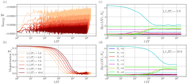
Figure 5: Dynamical detection of $U(1)\to\mathbb{Z}_{2}$ HS with Floquet drives. (a) Time evolution of the density of energy $\overline{E}=\overline{\left\langle Q^{(0)}\right\rangle}/L$. We show the energy prethermal plateau where energy is quasi-conserved. However, for a small system, it is difficult to fully thermalize under the Floquet drive even at long times due to finite-size effects. (b) Dynamics of the density of magnetization $\overline{S_{z}}=\overline{\left\langle\sum_{i}\sigma_{i}^{z}\right\rangle}/L$. The lifetime of $U(1)$ plateau is prolonged with increasing driving frequency. (c),(d) The time evolution of the participation entropy for $1/(JT)=5.0,10.0$ $N_{\downarrow}$ represents number of downwards spins. The state has weight mainly in the even magnetization sector, showing the $\mathbb{Z}_{2}$ plateau. Dashed lines represent participation entropy at infinite temperature. The parameters are $L=14$ with symmetry-breaking perturbation strength $\delta_{x}/J=10.0$. The numerical simulations are performed using exact diagonalization and 20 random realizations are used to compute the ensemble average over different initial states.

C.3 Effective Hamiltonian for $U(1)\to\mathbb{Z}_{2}\to E$ with random drives

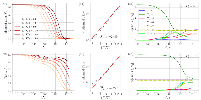
Figure 6: Dynamical detection of $U(1)\to\mathbb{Z}_{2}\to E$ HS with RMD. (a1) The time evolution of magnetization density $\overline{S_{z}}=\overline{\left\langle\sum_{i}\sigma_{i}^{z}\right\rangle}/L$. The quasi-conserved magnetization shows the $U(1)$ plateau. (a2) The time evolution of the expectation value of the parity $\overline{P_{z}}=\left\langle\prod_{i}\sigma_{i}^{z}\right\rangle$. The quasi-conserved parity shows the $\mathbb{Z}_{2}$ plateau. The breaking of early conservation is suppressed with increasing drive frequency. (b1),(b2) The scaling of the prethermal lifetime of the $U(1)$ plateau and the $\mathbb{Z}_{2}$ plateau $\tau_{m}\sim T^{-2.419},\;\tau_{p}\sim T^{-4.277}$ respectively, shows that the lifetime of HS can be dynamically prolonged by increasing the drive frequency. (c1),(c2) The time evolution of the participation entropy at drive frequencies $1/JT=5.0$ and $1/JT=15.0$, showing the distribution of state in each block. The Dashed lines represent the corresponding participation entropies at infinite temperature. The curves at low drive frequencies eventually coincide with the dashed lines, indicating that the system effectively heats up to an infinite-temperature state. The system size $L=14$, the symmetry-breaking perturbations are $\delta_{x}/J=10.0,\epsilon/J=6.0$. The numerical simulations are performed using exact diagonalization and 20 random realizations of the driving protocol and initial state are used to compute the ensemble average. The difference in simulation results between different realizations is very small, so we don’t need too many realizations.

Finite size effect becomes less notable if we switch to random drives. We still use the same kick generators ($H_{2,1}$) as defined above in the Floquet case. However, the $\mathbb{Z}_{2}$ breaking term can occur randomly in time. More concretely, we consider

$$H_{0}^{\pm}=(\delta_{x}\pm\epsilon)\sum_{i}\sigma_{i}^{x}.$$ (65)

and the evolution operator is redefined as

$$U_{\pm}=U\left(-H_{0}^{\pm},H_{1},H_{2}|\frac{T}{6}\right)U\left(H_{0}^{\pm},-H_{1},H_{2}|\frac{T}{6}\right).$$ (66)

The $U_{\pm}$ are then randomly aligned to form a stochastic drive sequence. Similar to the discussion in the Floquet case, the effective Hamiltonian $Q_{\pm}$ of the evolution operator $U_{\pm}$ has the same HS structure; in particular, we have $Q_{-}^{(0),(1)}=Q_{+}^{(0),(1)}$, but the randomness affects the $\mathbb{Z}_{2}$ plateau since $Q_{-}^{(2)}\neq Q_{+}^{(2)}$.

Once again, we perform a numerical simulation for a system of $L=14$ spins, starting from a Haar-random initial state within the $z$-magnetization sector $N_{\downarrow}=4$; this is a high-temperature (i.e., energy density) state. In Fig. 6(a1) and (a2), the system shows two clear prethermal plateaus corresponding to the U(1) and $\mathbb{Z}_{2}$ symmetries. We can clearly see the HS is well achieved dynamically through our protocol. In Fig. 6(c1) and (c2), we also show the $Z_{2}$ plateau exhibited by the participation entropy, during which the state is mainly distributed over the even magnetization sectors. At infinite times, the system will eventually fully thermalize, as indicated by the data in Fig. 6(c1), and the curve of participation entropy will reach the dashed line corresponding to a fully thermalized state. Note that at small driving frequencies, the $Z_{2}$ symmetry breaking already kicks in at early times, but this effect can be pushed to parametrically longer times with increasing drive frequency. We define the lifetimes $\tau_{m}$ and $\tau_{p}$ as the time for $\bar{S}_{z}$ and $\bar{P}_{z}$ to decay to $e^{-1}$ of their initial values in Fig. 6(a1) and (a2). In Fig. 6(b1) and (b2), we numerically show that the time scaling of the lifetimes $\tau_{m}$ and $\tau_{p}$ are approximately $\tau_{m}\sim T^{-2.419},\;\tau_{p}\sim T^{-4.255}$. The lifetime of the U(1) plateau approximately agrees well with the FGR scaling $T^{-2}$. The observed deviation is mainly due to the drive frequency not being large enough, where the $\mathbb{Z}_{2}$-breaking term is of comparable absolute magnitude to the leading order term $\mathbb{Z}_{2}$-preserving term (cf. Sec. B); thus, the next leading-order term will affect the dynamics during the U(1) plateau, which can be observed in the early-time dynamics of both the parity operator and the participation entropy. We emphasize that since the parity operator is a non-local operator, its dynamics may not be described by FGR. However, the numerical data clearly shows that the $\mathbb{Z}_{2}$-plateau lifetime can be parametrically controlled by modulating the drive frequency.

Appendix D HS in $Z_{4}$ Quantum Clock Model

In this section, we give the details of the effective Hamiltonian corresponding to the HS ladder that implements the $\mathbb{Z}_{4}$ quantum clock model. Consider the two Hamiltonians $H_{1}$ and $H_{0}$ that preserve the $\mathbb{Z}_{4}$ and $\mathbb{Z}_{2}$ symmetry, respectively:

$$H_{1} = \sum_{\langle i,j\rangle}J_{ij}\left(Z_{i}^{2}Z_{j}^{2}-\eta(e^{i\phi}Z_{i}^{\dagger}Z_{j}+\text{h.c.})\right)+\sum_{i}h_{i}\left(Z_{i}^{2}-\frac{1}{2}\left(X_{i}+X_{i}^{\dagger}\right)\right)+\sum_{i}g_{i}X_{i}^{2},$$

$$H_{0} = \sum_{i=1}^{L}b_{i}(Z_{i}+Z_{i}^{\dagger}).$$ (67)

Following the driving protocol defined in Sec. III.2, the effective Hamiltonian over four drive periods, $U_{F}^{4}=e^{-iQ4T}$, is:

$$Q=Q^{(0)}+Q^{(1)}+Q^{(2)}+\mathcal{O}(T^{3}),$$ (68)

$$Q^{(0)}=\frac{1}{2}\sum_{\langle i,j\rangle}J_{ij}\left(Z_{i}^{2}Z_{j}^{2}-\eta(e^{i\phi}Z_{i}^{\dagger}Z_{j}+e^{-i\phi}Z_{i}Z_{j}^{\dagger})\right)+\frac{1}{2}\sum_{i}g_{i}X_{i}^{2}-\frac{1}{2}\sum_{i}h_{i}(X_{i}+X_{i}^{\dagger}),$$

$$Q^{(1)}=\frac{iT}{16}\sum_{i}h_{i}^{2}[Z_{i}^{2},X_{i}+X_{i}^{\dagger}],$$

$$Q^{(2)}=\frac{T^{2}}{128}\left([Q^{(0)},[Q^{(0)},\sum_{l}b_{l}((2-i)Z_{l}+(2+i)Z_{l}^{\dagger})]]+\frac{1}{2}[\sum_{l}h_{l}Z_{l}^{2},[Q^{(0)},\sum_{m}b_{m}((1-i)Z_{m}+(1+i)Z_{m}^{\dagger})]]\right).$$

A Hamiltonian $\mathcal{O}$ is $Z_{4}$ and $Z_{2}$-preserving when $[\mathcal{O},\prod_{i}X_{i}]=0$ and $[\mathcal{O},\prod_{i}X_{i}^{2}]=0$. Clearly $[Q^{(0)},\prod_{i}X_{i}]=0;\;[Q^{(1)},\prod_{i}X_{i}]\neq 0,\;[Q^{(1)},\prod_{i}X_{i}^{2}]=0;\;[Q^{(2)},\prod_{i}X_{i}]\neq 0,\;[Q^{(2)},\prod_{i}X_{i}^{2}]\neq 0$, showing the $\mathbb{Z}_{4}\to\mathbb{Z}_{2}\to E$ HS.

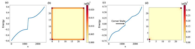
Figure 7: Energy spectrum and zero energy state of TI and HOTI. (a),(c) Energy spectrum of $Q^{(0)}$ and $Q^{(0)}+Q^{(1)}$ respectively. (b),(d) Density distribution corresponding to the zero energy mode of $Q^{(0)}$ and $Q^{(0)}+Q^{(1)}$ respectively (e.g., edge state and corner state). The parameters are $M=1.0,t=1.0,\Delta_{0}=1.0,\Delta_{1}=7.0$, system size is $L=19$.

Appendix E High-order Topological Insulators from HS

In this section, we elaborate on the HS setup implementing a change of topology from a TI to a HOTI. We give explicit expressions for the representation of the generating Hamiltonians in real space proposed in the main text for a possible experimental realization.

$$H_{2} = \frac{M}{2}\sum_{\vec{r},\alpha=0,1}(-1)^{\alpha}c^{\dagger}_{\vec{r},\alpha}c_{\vec{r},\alpha}+\sum_{\vec{r},\alpha=0,1}\sum_{j=x,y}\left(\frac{J}{2}(-1)^{\alpha}c^{\dagger}_{\vec{r}+\vec{e}_{j},\alpha}c_{\vec{r},\alpha}+\frac{\Delta_{0}}{2i}c^{\dagger}_{\vec{r}+\vec{e}_{j},\alpha+1}\sigma_{j}c_{\vec{r},\alpha}\right)+\text{h.c.},$$

$$H_{1} = \Delta_{1}\sum_{\vec{r},\alpha=0,1}(-1)^{\alpha}c^{\dagger}_{\vec{r},\alpha}(\sigma_{x}+\sigma_{y})c_{\vec{r},\alpha},$$

$$H_{1}^{\prime} = \Delta_{1}\sum_{\vec{r},\alpha=0,1}(-1)^{\alpha}c^{\dagger}_{\vec{r},\alpha}\sigma_{z}c_{\vec{r},\alpha},$$

$$H_{0} = \Delta_{2}\sum_{\vec{r},\alpha=0,1}c_{\vec{r},\alpha+1}^{\dagger}\sigma_{y}c_{\vec{r},\alpha},$$ (69)

where $c_{\vec{r},\alpha}=(c_{\vec{r},\alpha,\uparrow},c_{\vec{r},\alpha,\downarrow})$. We can also convert the fermionic orbital as well as the spin degrees of freedom equivalently into four sites in each unit cell $(c_{\vec{r},0,\uparrow},c_{\vec{r},0,\downarrow},c_{\vec{r},1,\uparrow},c_{\vec{r},1,\downarrow})\to(c_{\vec{r},0},c_{\vec{r},1},c_{\vec{r},2},c_{\vec{r},3})$. The protocol is thus also possibly realizable in ultra-cold atomic systems.

Figure 8: HOTI results when the initial state is the zero-energy eigenstate of $Q^{(0)}$ (i.e., edge state ). (a) Time evolution of the electron density at corner and edge ($n_{\text{corner}}=(n{(0,0)}+n{(L,L)})/2,\;n_{\text{edge}}=2\sum_{i=L/4}^{3L/4}n{(i,0)}/L$) without $\mathcal{I}$-breaking perturbation in $Q^{(1)}$ (marked by ’corner’ and ’edge’ labels in legend) and with $\mathcal{I}$-breaking perturbation (’corner SB’ and ’edge SB’ labels). When $\mathcal{I}$ is preserved in the first order effective Hamiltonian, density distribution at corners has a longer lifetime showing the existence of corner state. (b) Time evolution of electron density at the edge without $\mathcal{I}$-breaking perturbation for different drive frequency $1/T$. The lifetime of the boundary state (i.e., the first plateau) is significantly prolonged with increasing driving frequency. The system size is $L=19$ and the parameters are $M/J=1.0$, $\Delta_{0}/J=1.0$, $\Delta_{1}/J=7.0$, and $\Delta_{2}/J=12.0$.

With the evolution operator defined in Eq. (III.3), the effective Hamiltonian $U_{F}\equiv e^{-iQT}$ is

$$Q = Q^{(0)}+Q^{(1)}+\mathcal{O}(T^{2}),\ \ Q^{(0)}=\frac{1}{5}H_{2},\ \ Q^{(1)}=-\frac{iT}{200}([H_{1},H_{1}^{\prime}]+2[H_{1}+H_{1}^{\prime},H_{2}]).$$ (70)

$Q^{(0)}\propto H_{2}$ is a standard Hamiltonian for a TI. As what we discuss in Sec. A.4, the commutator of $H_{1}$ and $H_{1}^{\prime}$ in $Q^{(1)}$ introduces an on-site $\mathcal{T}$-breaking but $\mathcal{I}$-preserving perturbation which opens the energy gap and leaves two degenerate zero-energy corner states. In Fig. 7 we present the energy spectrum and the density distribution of the zero-energy eigenstates of $Q^{(0)}$ and $Q^{(0)}+Q^{(1)}$, respectively. We can clearly see the boundary states that characterize these two topological states of matter.

In the main text, we initialize the system as a product state with a large spatial support on the edge. Such a state can be experimentally prepared, for instance, by using cold atoms in optical lattices. We expect to observe a plateau of the particle density around the edge, which should be more pronounced by increasing the driving frequency, such that $Q^{(0)}$ dominates the early time evolution. However, technically, it is difficult to show a clear plateau because this product state can delocalize quickly into the bulk, and the remaining population around the edge is comparably weak, even in the absence of the first-order perturbation $Q^{(1)}$. To confirm the existence of this plateau, here we supply numerical simulation of the dynamics by starting from the zero-energy eigenstate of $Q^{(0)}$ (i.e., the edge states), such that only higher-order perturbations delocalizes the system. As shown in Fig. 8(a), as we increase the drive frequency, the decay of the electron density at the boundary slows down accordingly, revealing the first plateau of $Q^{(0)}$. In Fig. 8.(b), we show the time evolution of the electron density at the corners and boundaries with and without an $\mathcal{I}$-breaking perturbation. In the presence of the perturbation, labeled by ’corner SB’ and ’edge SB’, the density distribution on the corners decays quickly and agrees with the density distribution on the edges at long times. However, without the $\mathcal{I}$-breaking perturbation, the lifetime of the density distribution at the corners is visibly prolonged by an order of magnitude.

References

• Landau and Lifshitz [2013] L. D. Landau and E. M. Lifshitz, Statistical Physics: Volume 5, Vol. 5 (Elsevier, 2013).
• Chaikin et al. [1995] P. M. Chaikin, T. C. Lubensky, and T. A. Witten, Principles of condensed matter physics, Vol. 10 (Cambridge university press Cambridge, 1995).
• Pollmann et al. [2012] F. Pollmann, E. Berg, A. M. Turner, and M. Oshikawa, Symmetry protection of topological phases in one-dimensional quantum spin systems, Physical review b 85, 075125 (2012).
• Chen et al. [2013] X. Chen, Z.-C. Gu, Z.-X. Liu, and X.-G. Wen, Symmetry protected topological orders and the group cohomology of their symmetry group, Physical Review B 87, 155114 (2013).
• Anderson [1952] P. W. Anderson, An approximate quantum theory of the antiferromagnetic ground state, Physical Review 86, 694 (1952).
• Dine et al. [1981] M. Dine, W. Fischler, and M. Srednicki, A simple solution to the strong cp problem with a harmless axion, Physics letters B 104, 199 (1981).
• Brauner [2010] T. Brauner, Spontaneous symmetry breaking and nambu–goldstone bosons in quantum many-body systems, Symmetry 2, 609 (2010).
• Castelnovo et al. [2012] C. Castelnovo, R. Moessner, and S. L. Sondhi, Spin ice, fractionalization, and topological order, Annu. Rev. Condens. Matter Phys. 3, 35 (2012).
• Abanin et al. [2015] D. A. Abanin, W. De Roeck, and F. Huveneers, Exponentially slow heating in periodically driven many-body systems, Physical review letters 115, 256803 (2015).
• Kuwahara et al. [2016] T. Kuwahara, T. Mori, and K. Saito, Floquet–magnus theory and generic transient dynamics in periodically driven many-body quantum systems, Annals of Physics 367, 96 (2016).
• Bertini et al. [2021] B. Bertini, F. Heidrich-Meisner, C. Karrasch, T. Prosen, R. Steinigeweg, and M. Žnidarič, Finite-temperature transport in one-dimensional quantum lattice models, Reviews of Modern Physics 93, 025003 (2021).
• Martinez et al. [2016] E. A. Martinez, C. A. Muschik, P. Schindler, D. Nigg, A. Erhard, M. Heyl, P. Hauke, M. Dalmonte, T. Monz, P. Zoller, et al., Real-time dynamics of lattice gauge theories with a few-qubit quantum computer, Nature 534, 516 (2016).
• Ji et al. [2020] W. Ji, L. Zhang, M. Wang, L. Zhang, Y. Guo, Z. Chai, X. Rong, F. Shi, X.-J. Liu, Y. Wang, et al., Quantum simulation for three-dimensional chiral topological insulator, Physical Review Letters 125, 020504 (2020).
• Jepsen et al. [2021] P. N. Jepsen, W. W. Ho, J. Amato-Grill, I. Dimitrova, E. Demler, and W. Ketterle, Transverse spin dynamics in the anisotropic heisenberg model realized with ultracold atoms, Physical Review X 11, 041054 (2021).
• Oka and Kitamura [2019] T. Oka and S. Kitamura, Floquet engineering of quantum materials, Annual Review of Condensed Matter Physics 10, 387 (2019).
• Schweizer et al. [2019] C. Schweizer, F. Grusdt, M. Berngruber, L. Barbiero, E. Demler, N. Goldman, I. Bloch, and M. Aidelsburger, Floquet approach to z2 lattice gauge theories with ultracold atoms in optical lattices, Nature Physics 15, 1168 (2019).
• Geier et al. [2021] S. Geier, N. Thaicharoen, C. Hainaut, T. Franz, A. Salzinger, A. Tebben, D. Grimshandl, G. Zürn, and M. Weidemüller, Floquet hamiltonian engineering of an isolated many-body spin system, Science 374, 1149 (2021).
• Petiziol et al. [2022] F. Petiziol, S. Wimberger, A. Eckardt, and F. Mintert, Non-perturbative floquet engineering of the toric-code hamiltonian and its ground state, arXiv preprint arXiv:2211.09724  (2022).
• Kalinowski et al. [2023] M. Kalinowski, N. Maskara, and M. D. Lukin, Non-abelian floquet spin liquids in a digital rydberg simulator, Physical Review X 13, 031008 (2023).
• Jin et al. [2023] H.-K. Jin, J. Knolle, and M. Knap, Fractionalized prethermalization in a driven quantum spin liquid, Physical Review Letters 130, 226701 (2023).
• Sun et al. [2023] B.-Y. Sun, N. Goldman, M. Aidelsburger, and M. Bukov, Engineering and probing non-abelian chiral spin liquids using periodically driven ultracold atoms, PRX Quantum 4, 020329 (2023).
• Kitagawa et al. [2010] T. Kitagawa, E. Berg, M. Rudner, and E. Demler, Topological characterization of periodically driven quantum systems, Physical Review B 82, 235114 (2010).
• Potter et al. [2016] A. C. Potter, T. Morimoto, and A. Vishwanath, Classification of interacting topological floquet phases in one dimension, Physical Review X 6, 041001 (2016).
• Titum et al. [2016] P. Titum, E. Berg, M. S. Rudner, G. Refael, and N. H. Lindner, Anomalous floquet-anderson insulator as a nonadiabatic quantized charge pump, Physical Review X 6, 021013 (2016).
• Khemani et al. [2016] V. Khemani, A. Lazarides, R. Moessner, and S. L. Sondhi, Phase structure of driven quantum systems, Physical review letters 116, 250401 (2016).
• Else et al. [2016] D. V. Else, B. Bauer, and C. Nayak, Floquet time crystals, Physical review letters 117, 090402 (2016).
• Yao et al. [2017] N. Y. Yao, A. C. Potter, I.-D. Potirniche, and A. Vishwanath, Discrete time crystals: Rigidity, criticality, and realizations, Physical review letters 118, 030401 (2017).
• Else et al. [2020] D. V. Else, W. W. Ho, and P. T. Dumitrescu, Long-lived interacting phases of matter protected by multiple time-translation symmetries in quasiperiodically driven systems, Physical Review X 10, 021032 (2020).
• Dumitrescu et al. [2022] P. T. Dumitrescu, J. G. Bohnet, J. P. Gaebler, A. Hankin, D. Hayes, A. Kumar, B. Neyenhuis, R. Vasseur, and A. C. Potter, Dynamical topological phase realized in a trapped-ion quantum simulator, Nature 607, 463 (2022).
• Zhang et al. [2022] X. Zhang, W. Jiang, J. Deng, K. Wang, J. Chen, P. Zhang, W. Ren, H. Dong, S. Xu, Y. Gao, et al., Digital quantum simulation of floquet symmetry-protected topological phases, Nature 607, 468 (2022).
• Mi et al. [2022] X. Mi, M. Ippoliti, C. Quintana, A. Greene, Z. Chen, J. Gross, F. Arute, K. Arya, J. Atalaya, R. Babbush, et al., Time-crystalline eigenstate order on a quantum processor, Nature 601, 531 (2022).
• D’Alessio et al. [2016] L. D’Alessio, Y. Kafri, A. Polkovnikov, and M. Rigol, From quantum chaos and eigenstate thermalization to statistical mechanics and thermodynamics, Advances in Physics 65, 239 (2016).
• Vidmar and Rigol [2016] L. Vidmar and M. Rigol, Generalized gibbs ensemble in integrable lattice models, Journal of Statistical Mechanics: Theory and Experiment 2016, 064007 (2016).
• Hainaut et al. [2018] C. Hainaut, I. Manai, J.-F. Clément, J. C. Garreau, P. Szriftgiser, G. Lemarié, N. Cherroret, D. Delande, and R. Chicireanu, Controlling symmetry and localization with an artificial gauge field in a disordered quantum system, Nature communications 9, 1382 (2018).
• Haldar et al. [2018] A. Haldar, R. Moessner, and A. Das, Onset of floquet thermalization, Physical Review B 97, 245122 (2018).
• Agrawal et al. [2022] U. Agrawal, A. Zabalo, K. Chen, J. H. Wilson, A. C. Potter, J. Pixley, S. Gopalakrishnan, and R. Vasseur, Entanglement and charge-sharpening transitions in u (1) symmetric monitored quantum circuits, Physical Review X 12, 041002 (2022).
• Murthy et al. [2023] C. Murthy, A. Babakhani, F. Iniguez, M. Srednicki, and N. Y. Halpern, Non-abelian eigenstate thermalization hypothesis, Physical Review Letters 130, 140402 (2023).
• Kranzl et al. [2023] F. Kranzl, A. Lasek, M. K. Joshi, A. Kalev, R. Blatt, C. F. Roos, and N. Y. Halpern, Experimental observation of thermalization with noncommuting charges, PRX Quantum 4, 020318 (2023).
• Luitz et al. [2020] D. J. Luitz, R. Moessner, S. Sondhi, and V. Khemani, Prethermalization without temperature, Physical Review X 10, 021046 (2020).
• Beatrez et al. [2023] W. Beatrez, C. Fleckenstein, A. Pillai, E. de Leon Sanchez, A. Akkiraju, J. Diaz Alcala, S. Conti, P. Reshetikhin, E. Druga, M. Bukov, et al., Critical prethermal discrete time crystal created by two-frequency driving, Nature Physics 19, 407 (2023).
• Trenkwalder et al. [2016] A. Trenkwalder, G. Spagnolli, G. Semeghini, S. Coop, M. Landini, P. Castilho, L. Pezze, G. Modugno, M. Inguscio, A. Smerzi, et al., Quantum phase transitions with parity-symmetry breaking and hysteresis, Nature physics 12, 826 (2016).
• García-Pintos et al. [2019] L. P. García-Pintos, D. Tielas, and A. Del Campo, Spontaneous symmetry breaking induced by quantum monitoring, Physical Review Letters 123, 090403 (2019).
• Kokail et al. [2019] C. Kokail, C. Maier, R. van Bijnen, T. Brydges, M. K. Joshi, P. Jurcevic, C. A. Muschik, P. Silvi, R. Blatt, C. F. Roos, et al., Self-verifying variational quantum simulation of lattice models, Nature 569, 355 (2019).
• Choi et al. [2020] J. Choi, H. Zhou, H. S. Knowles, R. Landig, S. Choi, and M. D. Lukin, Robust dynamic hamiltonian engineering of many-body spin systems, Phys. Rev. X 10, 031002 (2020).
• Tran et al. [2021] M. C. Tran, Y. Su, D. Carney, and J. M. Taylor, Faster digital quantum simulation by symmetry protection, PRX Quantum 2, 010323 (2021).
• Richter and Pal [2021] J. Richter and A. Pal, Simulating hydrodynamics on noisy intermediate-scale quantum devices with random circuits, Physical Review Letters 126, 230501 (2021).
• Keenan et al. [2023] N. Keenan, N. F. Robertson, T. Murphy, S. Zhuk, and J. Goold, Evidence of kardar-parisi-zhang scaling on a digital quantum simulator, npj Quantum Information 9, 72 (2023).
• Zhao et al. [2023] H. Zhao, M. Bukov, M. Heyl, and R. Moessner, Making trotterization adaptive and energy-self-correcting for nisq devices and beyond, PRX Quantum 4, 030319 (2023).
• Zhao et al. [2019] H. Zhao, F. Mintert, and J. Knolle, Floquet time spirals and stable discrete-time quasicrystals in quasiperiodically driven quantum many-body systems, Physical Review B 100, 134302 (2019).
• Lapierre et al. [2020] B. Lapierre, K. Choo, A. Tiwari, C. Tauber, T. Neupert, and R. Chitra, Fine structure of heating in a quasiperiodically driven critical quantum system, Physical Review Research 2, 033461 (2020).
• Wen et al. [2021] X. Wen, R. Fan, A. Vishwanath, and Y. Gu, Periodically, quasiperiodically, and randomly driven conformal field theories, Physical Review Research 3, 023044 (2021).
• Mori et al. [2021] T. Mori, H. Zhao, F. Mintert, J. Knolle, and R. Moessner, Rigorous bounds on the heating rate in thue-morse quasiperiodically and randomly driven quantum many-body systems, Physical Review Letters 127, 050602 (2021).
• Long et al. [2022] D. M. Long, P. J. Crowley, and A. Chandran, Many-body localization with quasiperiodic driving, Physical Review B 105, 144204 (2022).
• Nathan et al. [2022] F. Nathan, I. Martin, and G. Refael, Topological frequency conversion in weyl semimetals, Physical Review Research 4, 043060 (2022).
• He et al. [2023] G. He, B. Ye, R. Gong, Z. Liu, K. W. Murch, N. Y. Yao, and C. Zu, Quasi-floquet prethermalization in a disordered dipolar spin ensemble in diamond, Physical Review Letters 131, 130401 (2023).
• Zhao et al. [2021] H. Zhao, F. Mintert, R. Moessner, and J. Knolle, Random multipolar driving: Tunably slow heating through spectral engineering, Physical Review Letters 126, 040601 (2021).
• Guarnieri et al. [2022] G. Guarnieri, M. T. Mitchison, A. Purkayastha, D. Jaksch, B. Buča, and J. Goold, Time periodicity from randomness in quantum systems, Physical Review A 106, 022209 (2022).
• Note [1] The proof in A relies on the Baker-Campbell-Hausdorff (BCH) formula which is generalized to continuous drives via the Floquet-Magnus expansion. Since in the latter, the commutator structure decouples from the time-ordered integrals, HS can be engineered also for continuous drives.
• Bukov et al. [2015] M. Bukov, L. D’Alessio, and A. Polkovnikov, Universal high-frequency behavior of periodically driven systems: from dynamical stabilization to floquet engineering, Advances in Physics 64, 139 (2015).
• Mori et al. [2016] T. Mori, T. Kuwahara, and K. Saito, Rigorous bound on energy absorption and generic relaxation in periodically driven quantum systems, Physical review letters 116, 120401 (2016).
• Abanin et al. [2017] D. A. Abanin, W. De Roeck, W. W. Ho, and F. Huveneers, Effective hamiltonians, prethermalization, and slow energy absorption in periodically driven many-body systems, Physical Review B 95, 014112 (2017).
• Note [2] Note the difference in notation between $Q_{[M]}$ which denotes the effective IFE Hamiltonian truncated to order $M$, and $Q_{n}$ which conserves the symmetry group $G_{n}$.
• Note [3] Note that there is another $\mathbb{Z}_{2}$ generated by Px=\prod@\slimits@iσixsubscript𝑃𝑥\prod@subscript\slimits@𝑖subscriptsuperscript𝜎𝑥𝑖P_{x}=\prod@\slimits@_{i}\sigma^{x}_{i} which will not be broken by the drive. However, since this is not a subgroup of the $\mathbb{Z}_{2}$ generated by $P_{z}$, we do not consider it in the present HS example.
• Note [4] Such an initial state is a high-temperature state with respect to $Q_{\pm}^{(0)}$ as verified by the energy density which is close to zero.
• Note [5] These threshold values are chosen for numerical simplicity and the scaling exponent of the prethermal lifetime in the high-frequency regime should not depend on their specific choices.
• Surace et al. [2019] F. M. Surace, A. Russomanno, M. Dalmonte, A. Silva, R. Fazio, and F. Iemini, Floquet time crystals in clock models, Physical Review B 99, 104303 (2019).
• Schindler et al. [2018] F. Schindler, A. M. Cook, M. G. Vergniory, Z. Wang, S. S. Parkin, B. A. Bernevig, and T. Neupert, Higher-order topological insulators, Science advances 4, eaat0346 (2018).
• Note [6] Note that, since the system is non-interacting, heating to infinite temperature does not occur even at infinite times.
• Halimeh et al. [2023] J. C. Halimeh, M. Aidelsburger, F. Grusdt, P. Hauke, and B. Yang, Cold-atom quantum simulators of gauge theories, arXiv preprint arXiv:2310.12201  (2023).
• Faist et al. [2020] P. Faist, S. Nezami, V. V. Albert, G. Salton, F. Pastawski, P. Hayden, and J. Preskill, Continuous symmetries and approximate quantum error correction, Physical Review X 10, 041018 (2020).
• Lieu et al. [2020] S. Lieu, R. Belyansky, J. T. Young, R. Lundgren, V. V. Albert, and A. V. Gorshkov, Symmetry breaking and error correction in open quantum systems, Physical Review Letters 125, 240405 (2020).
• Zhu et al. [2023] G.-Y. Zhu, N. Tantivasadakarn, A. Vishwanath, S. Trebst, and R. Verresen, Nishimori’s cat: stable long-range entanglement from finite-depth unitaries and weak measurements, Physical Review Letters 131, 200201 (2023).
• Sun et al. [2021] H. Sun, B. Yang, H.-Y. Wang, Z.-Y. Zhou, G.-X. Su, H.-N. Dai, Z.-S. Yuan, and J.-W. Pan, Realization of a bosonic antiferromagnet, Nature Physics 17, 990 (2021).
• Wei et al. [2022] D. Wei, A. Rubio-Abadal, B. Ye, F. Machado, J. Kemp, K. Srakaew, S. Hollerith, J. Rui, S. Gopalakrishnan, N. Y. Yao, et al., Quantum gas microscopy of kardar-parisi-zhang superdiffusion, Science 376, 716 (2022).
• Watanabe et al. [2013] H. Watanabe, T. Brauner, and H. Murayama, Massive nambu-goldstone bosons, Physical Review Letters 111, 021601 (2013).
• Albert and Jiang [2014] V. V. Albert and L. Jiang, Symmetries and conserved quantities in lindblad master equations, Physical Review A 89, 022118 (2014).
• Mori [2018] T. Mori, Floquet prethermalization in periodically driven classical spin systems, Physical Review B 98, 104303 (2018).
• Mori [2023] T. Mori, Floquet states in open quantum systems, Annual Review of Condensed Matter Physics 14, 35 (2023).
• Sieberer et al. [2023] L. M. Sieberer, M. Buchhold, J. Marino, and S. Diehl, Universality in driven open quantum matter, arXiv preprint arXiv:2312.03073  (2023).
• Howell et al. [2019] O. Howell, P. Weinberg, D. Sels, A. Polkovnikov, and M. Bukov, Asymptotic prethermalization in periodically driven classical spin chains, Physical review letters 122, 010602 (2019).
• Pizzi et al. [2021] A. Pizzi, A. Nunnenkamp, and J. Knolle, Classical prethermal phases of matter, Physical Review Letters 127, 140602 (2021).
• Ye et al. [2021] B. Ye, F. Machado, and N. Y. Yao, Floquet phases of matter via classical prethermalization, Physical Review Letters 127, 140603 (2021).
• Yue and Cai [2023] M. Yue and Z. Cai, Prethermal time-crystalline spin ice and monopole confinement in a driven magnet, Physical Review Letters 131, 056502 (2023).
• Yan et al. [2023] J. Yan, R. Moessner, and H. Zhao, Prethermalization in aperiodically kicked many-body dynamics, arXiv preprint arXiv:2306.16144  (2023).
• Buča and Prosen [2012] B. Buča and T. Prosen, A note on symmetry reductions of the lindblad equation: transport in constrained open spin chains, New Journal of Physics 14, 073007 (2012).
• Surace and Motrunich [2023] F. M. Surace and O. Motrunich, Weak integrability breaking perturbations of integrable models, Phys. Rev. Res. 5, 043019 (2023).
• Ikeda and Polkovnikov [2021] T. N. Ikeda and A. Polkovnikov, Fermi’s golden rule for heating in strongly driven floquet systems, Physical Review B 104, 134308 (2021).
• Yeh et al. [2023] H.-C. Yeh, A. Rosch, and A. Mitra, Decay rates of almost strong modes in floquet spin chains beyond fermi’s golden rule, Phys. Rev. B 108, 075112 (2023).