ProSparse: Introducing and Enhancing Intrinsic Activation Sparsity
within Large Language Models

Abstract

Activation sparsity refers to the existence of considerable weakly-contributed elements among activation outputs. As a prevalent property of the models using the ReLU activation function, it has been proven a promising paradigm to boost model inference efficiency. Nevertheless, most large language models (LLMs) adopt activation functions without intrinsic activation sparsity (e.g., GELU and Swish). Some recent efforts have explored introducing ReLU or its variants as the substitutive activation function to help LLMs achieve activation sparsity and inference acceleration, but few can simultaneously obtain high sparsity and comparable model performance. This paper introduces an effective sparsification method named “ProSparse” to push LLMs for higher activation sparsity without decreasing model performance. Specifically, after substituting the activation function of LLMs with ReLU, ProSparse adopts progressive sparsity regularization with a factor smoothly increasing along sine curves in multiple stages. This can enhance activation sparsity and alleviate performance degradation by avoiding radical shifts in activation distribution. With ProSparse, we obtain high sparsity of 89.32% and 88.80% for LLaMA2-7B and LLaMA2-13B, respectively, achieving comparable performance to their original Swish-activated versions. Our inference acceleration experiments further demonstrate the practical acceleration brought by higher activation sparsity.

1 Introduction

Recent years have witnessed the significant breakthrough made by large language models (LLMs), and these LLMs display commendable performance across a wide range of NLP tasks Brown et al. (2020); Wei et al. (2021); Ouyang et al. (2022); OpenAI (2023); Touvron et al. (2023a, b); Achiam et al. (2023). Nevertheless, the formidable computational costs required by LLM deployment and inference pose a considerable challenge to the wider application of LLMs Aminabadi et al. (2022); Pope et al. (2023). Among various techniques for handling this challenge, the utilization of activation sparsity is a promising one, for its effectiveness in enhancing inference efficiency Liu et al. (2023); Song et al. (2023) by leveraging the weakly-contributed elements among the outputs of LLM activation functions.

Using ReLU, which naturally outputs zero elements, as the activation function is a straightforward method to achieve intrinsic activation sparsity and widely adopted in early LLMs Raffel et al. (2020); Zhang et al. (2022a). However, recent LLMs predominantly favor GELU and Swish Touvron et al. (2023a); Chowdhery et al. (2023); Almazrouei et al. (2023), and thus lack intrinsic activation sparsity. To pursue the sparsity-based inference acceleration, ReLUfication Zhang et al. (2022b); Mirzadeh et al. (2023) has been explored to introduce the ReLU-based intrinsic activation sparsity into non-ReLU LLMs. Preliminary ReLUfication methods Zhang et al. (2022b, 2024) directly substitute the activation functions of non-ReLU LLMs with ReLU. Since activation function substitution cannot overcome the inherent limitation imposed by the original non-ReLU activation distribution, Mirzadeh et al. (2023) further introduce the inserted and shifted ReLU functions to enforce higher sparsity through radically shifting the activation distribution. Despite the promise of ReLUfication, existing efforts fail to achieve satisfactory activation sparsity and risk performance degradation caused by ReLUfication.

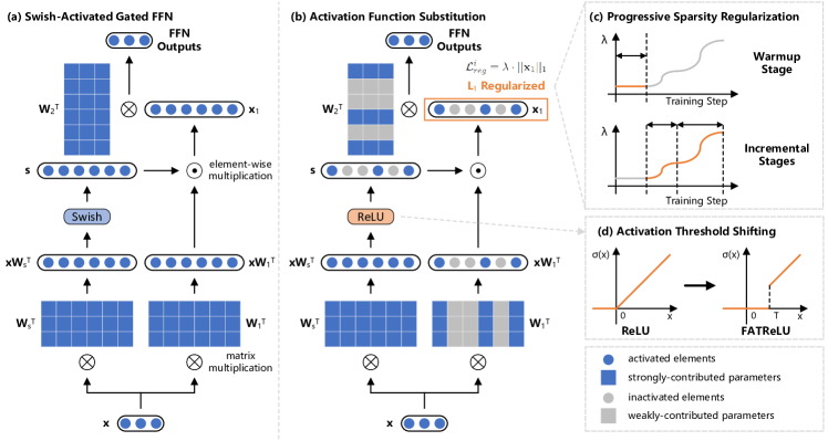
Figure 1: The overall architecture of ProSparse, which includes three steps: activation function substitution, progressive sparsity regularization, and activation threshold shifting.

In this paper, we propose an effective progressive ReLUfication method to help non-ReLU LLMs obtain high activation sparsity without compromising performance. We name the method “ProSparse”, which includes three steps shown in Figure 1: activation function substitution, progressive sparsity regularization, and activation threshold shifting. The first step is to replace the activation function of non-ReLU LLMs with ReLU and then apply continual training for adapting LLM to the new ReLU activation. As discussed above, this can hardly achieve satisfactory sparsity. Therefore, in the second step, we apply sparsity regularization Ma et al. (2019) to the intermediate activation outputs of the feed-forward networks (FFNs) within LLMs to seek higher activation sparsity. Considering the potential performance risks of forcing the fixed regularization factor Ma et al. (2019); Li et al. (2020), we progressively increase the regularization factor in multiple stages. Concretely, the factor is set to a low constant value for the warmup stage. Next, during each subsequent stage, the factor undergoes a gradual increase along a gentle sine curve. Following the cosine annealing learning rate scheduler Loshchilov and Hutter (2016), such progressive sparsity regularization can provide more time for the model to adapt to increasing regularization and avoid a radical shift in activation distribution, thereby alleviating performance degradation. The final step, inspired by FATReLU Kurtz et al. (2020), modifies the vanilla ReLU by shifting its activation threshold to a positive value. This prunes less influential neurons to further improve sparsity.

In our experiments, we apply ProSparse to the ReLUfication of LLaMA2 Touvron et al. (2023b). Activation sparsity of 89.32% and 88.80% are successfully achieved for LLaMA2-7B and LLaMA2-13B respectively, with performance comparable to original Swish-activated versions on various LLM benchmarks. Furthermore, we demonstrate the practical inference acceleration effect of higher activation sparsity by applying an approximate algorithm and an accurate algorithm to the inference of models with different sparsity. For the approximate one, we use PowerInfer Song et al. (2023), which achieves state-of-the-art speedup ratios tailored for sparsely-activated LLMs at the expense of potentially inaccurate inference due to the mistakes of activation predictors. For the accurate one, we implement two GPU operators that leverage the input-side and output-side sparsity during the computation of ReLU-activated FFN layers. The experimental results demonstrate that those models with higher sparsity can achieve more significant inference acceleration with both algorithms.

In summary, we make the following contributions in this paper: (1) We propose ProSparse, an effective ReLUfication method that converts non-ReLU LLMs into much sparser ReLU-activated LLMs without decreasing model performance. (2) Sparsely-activated versions of LLaMA2-7B and LLaMA2-13B comparable to their original Swish-activated versions in performance are both obtained and available. (3) We demonstrate the practical inference acceleration effect of higher activation sparsity that ProSparse can reach.

2 Related Works

Here we mainly introduce works on improving LLM inference efficiency. More details on LLMs can refer to the existing surveys Bommasani et al. (2021); Zhao et al. (2023). More related works about $L_{1}$ regularization are listed in Appendix A.

Despite the commendable performance of LLMs, the sustainable increase in the scale of model parameters brings the exponential growth of inference computations, making the deployment of LLMs a formidable challenge Kaplan et al. (2020); Liu et al. (2023). To reduce the computational costs required by the inference of such large models, various model compression methods have been proposed, such as quantization Han et al. (2015a); Jacob et al. (2018); Nagel et al. (2019); Zhao et al. (2019); Bai et al. (2022); Xiao et al. (2023); Yao et al. (2023), pruning Han et al. (2015a, b); Molchanov et al. (2016); Hoefler et al. (2021); Ma et al. (2023); Sun et al. (2023); Frantar and Alistarh (2023); Xia et al. (2023), and distillation Hinton et al. (2015); Tang et al. (2019); Touvron et al. (2021); Gu et al. (2023); Hsieh et al. (2023). Efficient sampling methods have also been proposed to achieve faster inference decoding speed Leviathan et al. (2023); Wang et al. (2023); Chen et al. (2023); Miao et al. (2023).

In general, none of the above methods involve leveraging the intrinsic mechanisms within LLMs to achieve inference acceleration. To this end, some recent works Li et al. (2022); Liu et al. (2023); Song et al. (2023) notice the intrinsic activation sparsity within some LLMs and exploit this sparsity for inference acceleration. Activation sparsity refers to the phenomenon where certain model parameters, corresponding to those zero or small elements in activation outputs, have a weak impact on final LLM outputs given a specific input. These weakly-contributed parameters are regarded as inactivated and can thus be skipped during inference to achieve sparse computation, without redundant computational resources spent on them. Therefore, the utilization of activation sparsity is orthogonal to model compression and efficient sampling, and these approaches can be easily accumulated.

Previous studies have marked activation sparsity as a prevalent phenomenon existing in almost any ReLU-activated Transformer architecture Li et al. (2022), from LLMs (e.g., T5 Raffel et al. (2020) and OPT Zhang et al. (2022a)) to some vision models (e.g., ViT Dosovitskiy et al. (2020)). However, recent LLMs such as Falcon Almazrouei et al. (2023) and LLaMa Touvron et al. (2023b) prevalently adopt non-ReLU activation functions such as GELU Hendrycks and Gimpel (2016) and Swish Elfwing et al. (2018) and do not exhibit activation sparsity. Therefore, to leverage the merits of activation sparsity without training a ReLU-activated LLM from scratch, many works conduct ReLUfication, which introduces sparse ReLU-based activations into non-ReLU LLMs. Zhang et al. (2022b) train the GELU-activated BERT Devlin et al. (2018) into a ReLU-activated version after a direct substitution of the activation function. Zhang et al. (2024) apply a similar paradigm to Falcon and LLaMA, which are activated by GELU and Swish respectively. Since activation substitution cannot reach satisfactory sparsity, mainly due to the unhandled inherent limitation of the original non-ReLU activation distribution, Mirzadeh et al. (2023) introduce the inserted and shifted ReLU activation functions and conduct a radical shift in activation distribution. Although these shifted operations are claimed to achieve sparsity of nearly 95%, we cannot replicate the results in our experiments (Section 4.2) and the sparsity is still limited.

As discussed above, we can clearly recognize the promise of activation sparsity and also observe the key challenge of leveraging ReLUfication to achieve activation sparsity: how to concurrently achieve high sparsity and comparable performance. To this end, this paper introduces ProSparse, a ReLUfication method that can obtain high ReLU-based activation sparsity for non-ReLU LLMs without performance degradation.

3 Methodology

3.1 Definitions and Notations

For the convenience of subsequent demonstrations, here we define activation sparsity within LLMs in detail. Since the activation function mainly exists in the FFN layers of LLMs, we first formalize the computation process of FFNs. Given the hidden dimension $d_{model}$ and the FFN intermediate dimension $d_{ff}$, the computation process of a gated FFN (i.e., the most widely adopted FFN architecture in recent Transformer-based LLMs Dauphin et al. (2017); Shazeer (2020)) can be formalized as:

$$\mathbf{s}=\sigma(\mathbf{x}\mathbf{W}_{s}^{T}), \quad\mathbf{x}_{1}=\mathbf{s}\odot(\mathbf{x}\mathbf{W}_{1}^{T}),$$ (1)

$$\text{FFN}(\mathbf{x}) =\mathbf{x}_{1}\mathbf{W}_{2}^{T},$$

where $\mathbf{x}\in\mathbb{R}^{d_{model}}$, $\mathbf{s},\mathbf{x}_{1}\in\mathbb{R}^{d_{ff}}$, $\sigma$, and $\odot$ denote the input hidden states, the gating scores, the intermediate outputs, the activation function, and the element-wise multiplication respectively. $\mathbf{W}_{s},\mathbf{W}_{1}\in\mathbb{R}^{d_{ff}\times d_{model}}$ and $\mathbf{W}_{2}\in\mathbb{R}^{d_{model}\times d_{ff}}$ are learnable weights.

We define the activation sparsity (hereinafter abbreviated as sparsity) as the ratio of zero elements (i.e., inactivated elements) in $\mathbf{x}_{1}$ for a specific input $\mathbf{x}$. However, since the sparsity often varies in different layers for different inputs, we evaluate the sparsity of the whole LLM using the average sparsity, defined as the average value of sparsity across all layers in an LLM on a sufficiently large amount of input data.

In this paper, we focus on the task of ReLUfication, namely converting an LLM using a non-RELU activation function $\sigma$ (e.g., GELU or Swish) into a ReLU-activated one, while making the activation sparsity as high as possible and mitigating performance degradation.

3.2 Methodology of ProSparse

We propose ProSparse to achieve the above targets. In ProSparse, three steps are carefully designed to introduce and enhance the intrinsic activation sparsity for a non-ReLU LLM: (1) activation function substitution; (2) progressive sparsity regularization; (3) activation threshold shifting.

Activation Function Substitution

For lack of attention to activation sparsity, a majority of recent mainstream LLMs adopt non-ReLU activation functions such as GELU and Swish that output few zero elements (i.e., low activation sparsity according to the above definition). Therefore, the first step of ProSparse is to introduce intrinsic sparsity through activation function substitution, which replaces the FFN activation function $\sigma$ with ReLU, namely $\sigma(x)=\max(x,0)$, followed by continual training. This can make the ratio of zero activation elements significantly larger and preliminarily adapt the LLM to new ReLU activation.

Progressive Sparsity Regularization

Nevertheless, activation function substitution by nature does not change the activation distribution, which will potentially limit the sparsity to relatively low values. To push for higher sparsity, a typical method is $L_{1}$ sparsity regularization Li et al. (2022), which introduces the $L_{1}$ regularization loss as an extra training target. Given the intermediate output $\mathbf{x}_{1}$ of the $i$-th FFN layer in an LLM, the regularization loss is defined as:

$$\mathcal{L}_{reg}^{i}=\lambda\cdot||\mathbf{x}_{1}||_{1},$$ (2)

where $||\cdot||_{1}$ is the $L_{1}$ norm operator and $\lambda$ is the regularization factor. For an LLM with $K$ FFN layers, the total regularization loss is summed from the losses of all layers, namely $\mathcal{L}_{reg}=\sum_{i=1}^{K}\mathcal{L}_{reg}^{i}$.

Algorithm 1 The process of progressive sparsity regularization in ProSparse.

0:  The total number of stages $S\geq 1$.

0:  A sequence of peak $\lambda$ values $\{\lambda_{i}\}_{i=1}^{S}$, s.t. $0<\lambda_{1}\leq\lambda_{2}\leq...\leq\lambda_{S}$.

0:  Accumulated step numbers of respective stages $\{T_{i}\}_{i=1}^{S}$, s.t. $0<T_{1}<T_{2}<...<T_{S}$.

1:  // warmup stage

2:  for $t\leftarrow 1$ to $T_{1}$ do

3:     $\lambda\leftarrow\lambda_{1}$

4:  end for

5:  // incremental stages

6:  for $i\leftarrow 2$ to $S$ do

7:     for $t\leftarrow T_{i-1}+1$ to $T_{i}$ do

8:        $\eta\leftarrow\frac{1}{2}[\sin(-\frac{\pi}{2}+\frac{t-T_{i-1}}{T_{i}-T_{i-1}}\pi)+1]$

9:        $\lambda\leftarrow\lambda_{i-1}+\eta(\lambda_{i}-\lambda_{i-1})$

10:     end for

11:  end for

Considering the potentially unstable training and performance degradation due to fixed regularization factors Georgiadis (2019); Kurtz et al. (2020); Li et al. (2022), we propose the progressive sparsity regularization, where the factor $\lambda$ is carefully scheduled to gently increase in multiple stages, as displayed in Algorithm 1.

Concretely, for the warmup stage, we set $\lambda$ to a constant value, which is relatively small to prevent radical activation distribution shifts and introduce higher preliminary sparsity. Next, for each of the remaining stages (hereinafter called incremental stages), $\lambda$ is scheduled to increase along a smooth sine curve from a trough value to a peak value. Inspired by the cosine annealing scheduler for learning rates Loshchilov and Hutter (2016), we choose the sine function for $\lambda$ increase owing to its special trend. Specifically, the sine function has small derivatives near the trough and the peak, thereby $\lambda$ will not increase radically around these two points. This provides the LLMs with more time to adapt the activation distributions to the newly increased $L_{1}$ regularization. Notably, each stage is accompanied by certain steps of training. The step number and peak value of each stage are chosen according to the target sparsity and stability requirements.

Activation Threshold Shifting

As demonstrated by recent works, there exist considerable amounts of non-zero low elements in the activation outputs, which have little influence on final results and thus can be pruned for higher sparsity Zhang et al. (2024). Therefore, following FATReLU Kurtz et al. (2020), we modify the ReLU by shifting the activation threshold, i.e.,

$$\sigma(x)=\begin{cases}x\quad\mathrm{when}\ x\geq T,\\ 0\quad\mathrm{otherwise},\end{cases}$$ (3)

where $T>0$ is a positive threshold. As long as $T$ is properly chosen (see Appendix G), such an adjustment can increase sparsity with negligible losses Zhang et al. (2024).

3.3 Practical Inference Acceleration Test

To go further beyond former theoretical acceleration analyses based on FLOPs (Floating Point Operations Per Second) Mirzadeh et al. (2023) and establish the practical value of ProSparse, we compare the acceleration effects of LLMs with different sparsity on real GPU hardware. For comprehensiveness, we introduce two categories of acceleration algorithms based on activation sparsity: an approximate algorithm and an accurate algorithm.

Approximate Acceleration Algorithms

Utilizing activation sparsity, recent approximate acceleration algorithms predominantly rely on activation predictors, typically small neural networks, to forecast the activation distributions indicated by the sparse intermediate outputs $\mathbf{x}_{1}$ given a specific input $\mathbf{x}$ Liu et al. (2023); Song et al. (2023). In this way, they can make wiser hardware allocation or computation policies to avoid resource waste on weakly-contributed parameters. However, their efficiency and accuracy largely depend on the predictors’ performance, and invalid predictions can cause suboptimal hardware allocation or even inference inaccuracy.

Therefore, to test a sparse LLM’s practical acceleration value with approximate algorithms, we focus on three metrics: the activation recall (hereinafter abbreviated as recall), the predicted sparsity, and the inference speed. The former two metrics evaluate the performance of activation predictors as well as the activation predictability of a sparse LLM Zhang et al. (2024).

Concretely, the recall refers to the average ratio of correctly predicted activated elements among all the truly activated elements in $\mathbf{x}_{1}$. The predicted sparsity is calculated as the ratio of predicted inactivated elements among all the elements in $\mathbf{x}_{1}$. Predictors with higher recall and predicted sparsity can help an acceleration framework obtain a better grasp of activation distribution and thus make wiser policies for faster inference as well as low inference inaccuracies Liu et al. (2023).

For inference speed, we adopt PowerInfer Song et al. (2023), a state-of-the-art approximate algorithm as a representative to measure practical speedup ratios. Refer to Appendix B for more introductions of approximate algorithms.

Accurate Acceleration Algorithms

To achieve acceleration without potential inference inaccuracies, we implement two hardware-efficient sparse GPU operators with system-level optimizations, such as operator fusion, coalesced memory access, and vectorization, thereby exploiting input-side and output-side sparsity in Equation 1.

Concretely, we reorganize a ReLU-activated gated FFN into three major steps and our two operators are responsible for the step (2) and (3) respectively: (1) A dense matrix-vector multiplication operator $\mathbf{x}\mathbf{W}_{s}^{T}$ which can be directly supported by vendor libraries such as cuBLAS; (2) A fused operator of ReLU and $\mathbf{s}\odot(\mathbf{x}\mathbf{W}_{1}^{T})$ with output-side sparsity; (3) A sparse matrix-vector multiplication operator $\mathbf{x}_{1}\mathbf{W}_{2}^{T}$ with input-side sparsity.

We adopt the single-step speedup ratios of steps (2) and (3) with these two operators respectively to reflect the practical accurate acceleration potential of sparse LLMs. Refer to Appendix C for implementation details of our operators.

4 Experiments

Setting	Average	Code	Commonsense	Reading	GSM8K	MMLU	BBH	AGI Eval	Average
	Sparsity	Generation	Reasoning	Comprehension
Original-7B	-	16.37	69.59	61.87	12.96	44.45	32.96	27.53	37.96
ReluLLaMA-7B	66.98	15.85	69.64	70.54	5.84	38.64	35.07	27.73	37.62
Vanilla ReLU-7B	66.04	21.31	70.73	73.22	11.22	49.22	36.11	28.01	41.40
Shifted ReLU-7B	69.59	20.50	70.09	73.17	13.87	48.54	35.20	27.94	41.33
Fixed $L_{1}$-7B	91.46	18.85	66.01	55.39	2.27	32.28	31.40	26.48	33.24
ProSparse-7B∗	88.11	19.47	66.29	63.33	12.74	45.21	33.59	27.55	38.31
ProSparse-7B	89.32	19.42	66.27	63.50	12.13	45.48	34.99	27.46	38.46
Original-13B	-	20.19	72.58	71.55	22.21	54.69	37.89	29.33	44.06
ReluLLaMA-13B	71.56	20.19	70.44	73.29	18.50	50.58	37.97	28.22	42.74
ProSparse-13B∗	87.97	29.03	69.75	67.54	25.40	54.78	40.20	28.76	45.07
ProSparse-13B	88.80	28.42	69.76	66.91	26.31	54.35	39.90	28.67	44.90

Table 1: The overall experimental results with comparisons of activation sparsity (%) and downstream performance (%). “Original” refers to the original Swish-activated LLaMA2 versions Touvron et al. (2023b). “ProSparse-7B^∗” and “ProSparse-13B^∗” denote the ProSparse versions without activation threshold shifting.

4.1 Experimental Settings

Pre-Training Datasets

We use a mixed dataset consisting of both language modeling datasets and instruction tuning datasets. The language modeling datasets are directly cleaned and filtered from raw corpus, including StarCoder Li et al. (2023), Wikipedia Wikimedia Foundation (2022), Pile Gao et al. (2020), and other collected datasets. The instruction tuning datasets mainly involve input instructions and annotated target answers, including UltraChat Ding et al. (2023), multiple-choice QA data of P3 Sanh et al. (2021) (Choice P3), PAQ Lewis et al. (2021), Unnatural Instructions Honovich et al. (2022), Flan Longpre et al. (2023), Super-Natural Instructions Wang et al. (2022), and other collected datasets.

Evaluation Benchmarks

To evaluate the task-specific performance of the LLMs obtained by ProSparse, we introduce the following benchmarks.

Code Generation: We compute the average pass@1 scores on HumanEval (0-shot) Chen et al. (2021) and MBPP (3-shot) Austin et al. (2021).

Commonsense Reasoning: We report the average 0-shot accuracies on PIQA Bisk et al. (2020), SIQA Sap et al. (2019), HellaSwag Zellers et al. (2019), WinoGrande Sakaguchi et al. (2020), and COPA Roemmele et al. (2011).

Reading Comprehension: We compute the average 0-shot accuracies on BoolQ Clark et al. (2019), 0-shot accuracy on LAMBADA Paperno et al. (2016) and TyDi QA Clark et al. (2020).

Other Popular Benchmarks: We report the average accuracies on GSM8K (8-shot) Cobbe et al. (2021), MMLU (5-shot) Hendrycks et al. (2020), Big Bench Hard (BBH) (3-shot) Suzgun et al. (2022), and AGI-Eval (0-shot) Zhong et al. (2023). Refer to Appendix I for more details.

4.2 Overall Results

With ProSparse, we conduct ReLUfication on Swish-activated LLaMA2-7B and LLaMA2-13B. To demonstrate the advantage of ProSparse, we introduce the following baseline methods:

Vanilla ReLU Zhang et al. (2024) simply replaces the Swish function with ReLU and introduces continual training to recover performance.

Shifted ReLU Mirzadeh et al. (2023) is used to break the bottleneck of vanilla ReLU for higher sparsity. Specifically, this is done by subtracting a constant scalar $b$ from the input hidden states before the ReLU operator: $\mathbf{s}=\mathrm{ReLU}(\mathbf{x}\mathbf{W}_{s}^{T}-b)$. This results in a radical left shift in the activation distribution and thus substantially boosts sparsity.

Fixed $L_{1}$ imposes an $L_{1}$ regularization loss on the basis of vanilla ReLU. Different from ProSparse, the regularization factor $\lambda$ is kept constant throughout the training process.

For fairness, all the average sparsity values are computed on the same mixed dataset for ProSparse pre-training and all models are trained with the same number of tokens. The value of $\lambda$ for fixed $L_{1}$ is set to the average value of the factor during the last incremental stage of ProSparse and the bias $b$ for shifted ReLU is tuned to ensure best performance. We also compare our models with the open ReluLLaMA and the original Swish-activated LLaMA2 versions. For more hyper-parameters, see Appendix appendices F, G and H.

Setting	Average	Activation	Predicted	PowerInfer	Speedup to	Step (2)	Step (2)	Step (3)	Step (3)
	Sparsity	Recall	Sparsity	Speed	ReluLLaMA	Time ($\downarrow$)	Speedup	Time ($\downarrow$)	Speedup
ReluLLaMA-7B	66.98	90.89	58.95	11.37	1.00	67.12	1.35	63.00	1.32
Vanilla ReLU-7B	66.04	87.72	72.57	12.04	1.06	67.85	1.33	63.28	1.31
Fixed $L_{1}$-7B	91.46	94.51	82.85	19.62	1.73	40.99	2.21	54.19	1.53
ProSparse-7B∗	88.11	93.46	75.24	16.30	1.43	46.66	1.94	55.56	1.49
ProSparse-7B	89.32	92.34	78.75	-	-	45.38	2.00	55.05	1.51
ReluLLaMA-13B	71.56	86.41	71.93	6.59	1.00	69.92	1.88	75.47	1.51
ProSparse-13B∗	87.97	91.02	77.93	8.67	1.32	55.29	2.38	67.50	1.68
ProSparse-13B	88.80	91.11	78.28	-	-	53.78	2.44	66.73	1.70

• $\dagger$ For reference, the average number of tokens generated by llama.cpp per second is about 3.67 for 7B and 1.92 for 13B. The average time for step (2) and (3) without sparse GPU operators is about 90.55 and 82.92 (us) for 7B, 131.36 and 113.68 (us) for 13B respectively under all sparsity. ProSparse versions with activation threshold shifting are not supported by PowerInfer at present. Note that Fixed $L_{1}$ suffers from severe performance degradation (See Table 1).

Table 2: The comparison of activation recalls (%), predicted sparsity (%), PowerInfer inference speeds (tokens per second), and single-step time (us) with our sparse GPU operators among LLMs with different sparsity. “Step (2)” and “Step (3)” correspond to the steps in Section 3.3. “Time” means the average wall-clock time (us) cost by each step with our sparse GPU operators, and “Speedup” is the speedup ratio to the setting without operators.

The results are shown in Table 1 (See Appendix E for performance on each independent benchmark). As demonstrated by the average sparsity and performance scores, ProSparse is the only ReLUfication method that simultaneously achieves high sparsity and comparable downstream performance to the original LLaMA2. By contrast, Vanilla ReLU and Shifted ReLU can give higher performance at the expense of low sparsity, while Fixed $L_{1}$ obtains the highest sparsity with significant performance degradation.

To delve deeper into the training dynamics of different ReLUfication methods, we plot the trends of sparsity for each method in Figure 2. (1) Among the settings involved, the trend of sparsity is incremental iff non-zero $L_{1}$ regularization is applied. (2) Though ProSparse does not achieve high sparsity at first, the warmup stage quickly produces a considerable sparsity increase, and then the sparsity consistently grows in a smooth trend. Finally, the activation threshold shifting makes a marginal contribution to sparsity. Such a stable increase in sparsity avoids radical activation disturbances and provides enough time for adapting the activation distribution, which is the key to ProSparse’s alleviated performance degradation.

4.3 Acceleration Effect of Sparsity

Approximate Acceleration Algorithm

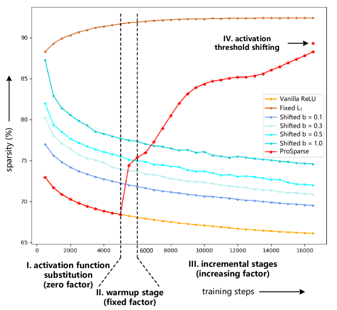
Figure 2: The trend of sparsity (7B models) along the training process. “Shifted” denotes Shited ReLU and $b=0.1$ corresponds to the results in Table 1.

In this section, we train the activation predictors for each sparse LLM obtained by the above ReLUfication methods and compare the recalls, predicted sparsity, and actual inference speeds on PowerInfer Song et al. (2023). As the FFN in each Transformer layer has different activation distributions as well as different predictors, the former two metrics are averaged from the results of all layers. Note that models with Shifted ReLU are not tested since PowerInfer and our sparse operators do not support this ReLU variant at present. Refer to Appendix D for training details of predictors.

As demonstrated by the results shown in Table 2, compared with llama.cpp, an acceleration framework without sparsity utilization, PowerInfer achieves no less than 3$\times$ speedup, revealing the significant potential of sparsity-based acceleration. Moreover, an increased activation sparsity can considerably improve the activation recall, the predicted sparsity, and the inference speed of PowerInfer. This proves the considerable practical values of even more sparsely activated LLMs in improving the inference speed with predictor-based approximate acceleration algorithms and mitigating the inaccurate inference problem. ProSparse, which reaches a high sparsity without performance degradation, can thus gain the most benefits.

Setting	Mixed	StarCoder	Wikipedia	Pile	UltraChat	Choice	PAQ	Flan	Unnatural	Super-Natural
						P3			Instructions	Instructions
ReluLLaMA-7B	66.98	66.60	67.16	67.35	67.91	67.35	66.98	67.35	66.42	66.98
Vanilla ReLU-7B	66.04	65.86	65.67	65.86	67.16	66.42	66.23	65.86	65.49	65.86
Shifted ReLU-7B	69.59	69.59	69.03	69.03	70.52	69.78	69.40	69.22	69.22	69.03
Fixed $L_{1}$-7B	91.46	91.23	87.97	87.97	95.45	99.33	98.58	93.52	96.20	98.01
ProSparse-7B∗	88.11	88.20	83.30	84.24	91.23	97.94	96.74	90.76	93.00	95.71
ProSparse-7B	89.32	89.13	84.33	85.35	93.66	98.33	97.28	91.74	93.80	96.32
ReluLLaMA-13B	71.56	71.33	71.45	71.56	72.27	71.80	71.21	71.56	70.85	71.33
ProSparse-13B∗	87.97	87.50	81.64	83.06	92.45	98.41	97.54	91.65	92.92	96.40
ProSparse-13B	88.80	88.63	83.65	84.12	92.65	98.73	97.99	92.54	93.66	96.92

Table 3: The average sparsity (%) on our mixed pre-training dataset (denoted as “Mixed”) and its components.

Accurate Acceleration Algorithm

Furthermore, with LLMs of different sparsity, we measure the average single-step wall-clock time spent by our two sparse GPU operators, which are responsible for step (2) and step (3) in Section 3.3 respectively. As demonstrated in Table 2, higher activation sparsity can make accurate algorithms based on GPU operators more efficient. Besides, our two sparse GPU operators also display satisfactory speedup ratios up to 2.44 and 1.70 respectively with better acceleration effects for larger models.

4.4 Dataset-Wise Analysis

Despite the satisfactory average sparsity, there still exist gaps between the mixed pre-training dataset and the actual input texts that the model will encounter in real-life applications. To investigate the sparsity of our model under different scenarios, we compute the sparsity on each component of the mixed dataset respectively.

As demonstrated in Table 3, the sparse LLMs obtained through $L_{1}$ regularization (i.e., Fixed $L_{1}$ and ProSparse) have a pronounced property of inconsistent dataset-wise sparsity. Concretely, the sparsity on instruction tuning datasets is significantly higher than those on language modeling datasets (i.e., StarCoder, Wikipedia, and Pile). Considering the contents of datasets, we come to the following assumption: the more formatted a dataset is, the higher sparsity $L_{1}$-regularized models can achieve. Plain text datasets including Wikipedia and Pile have the lowest sparsity, followed by the more formatted code dataset StarCoder. Among instruction tuning datasets, QA datasets (Choice P3 and PAQ) with the most monotonic input-output formats obtain the highest sparsity. By contrast, the sparsity is relatively lower on UltraChat and Flan, covering general dialogues and a wide variety of tasks respectively. Notably, dialogues and tasks with formatted instructions cover a majority of input contents of conversational AI, the mainstream application form of LLMs. Such higher sparsity on instruction tuning data will endow ProSparse with more significant practical values.

4.5 Layer-Wise Analysis

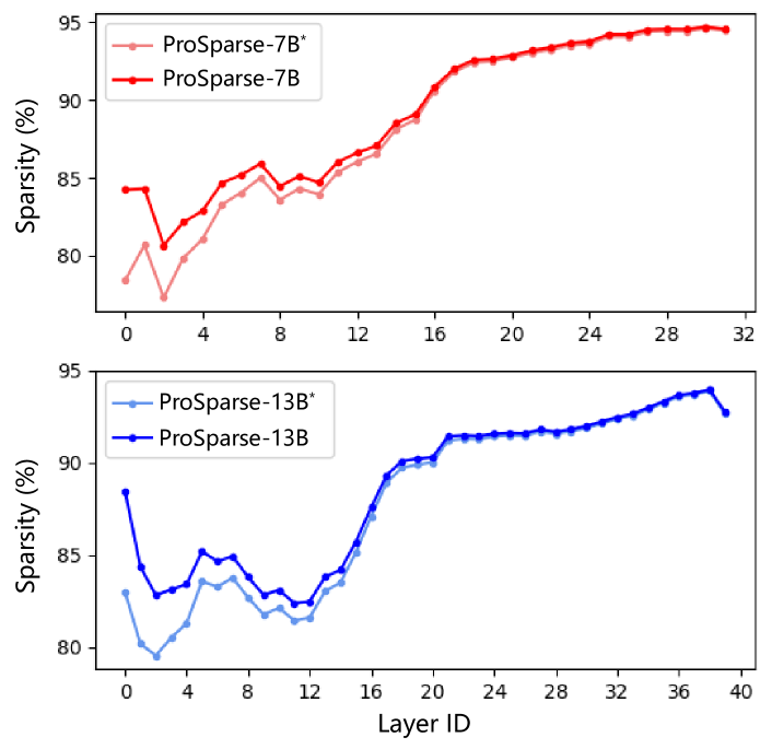
Figure 3: The layer-wise sparsity of ProSparse models. The marker “^∗” denotes the settings without activation threshold shifting.

Another problem worth concern is the layer-wise sparsity, which may potentially impact the load balance issue and the design of inference frameworks. Therefore, we compute the sparsity of each layer for ProSparse models, as shown in Figure 3.

From the tendency of the line chart, we clearly observe layer-wise sparsity imbalance in that lower layers are significantly denser than higher layers. Nevertheless, the activation threshold shifting can considerably improve the sparsity of lower layers with little impact on higher layers. Although this technique only contributes marginally to the average sparsity, it is still indispensable in alleviating the layer-wise sparsity imbalance issue.

5 Conclusion

In this work, we propose ProSparse, an effective ReLUfication method for introducing and enhancing intrinsic activation sparsity from non-ReLU LLM checkpoints without impairing performance. Extensive experiments not only demonstrate the advantage of ProSparse over existing methods but also reveal its practical values in inference acceleration with both approximate algorithms and accurate algorithms. Deeper analyses of the sparsity trends, dataset-wise sparsity, and layer-wise sparsity indicate the reasonableness of progressive sparsity regularization in smoothing training dynamics, the ProSparse’s high-sparsity bias for more practical instruction tuning datasets, and the effectiveness of activation threshold shifting in alleviating layer-wise sparsity imbalance.

Limitations

Firstly, the scales of LLMs involved in this work, including 7B and 13B, are relatively limited. For more comprehensive studies, both small-scale models (e.g., 2B or less) and huge-scale models (e.g., 70B or more) are supposed to be tested.

Next, we only focus on the sparsity-based acceleration of step (2) and step (3) of FFN, leaving a considerable ratio of LLM computation unoptimized. Actually, there already exist preliminary works in the sparsification of the attention layers Shen et al. (2023); Wortsman et al. (2023). For future works, we will continue to explore how to introduce and enhance sparsity in FFN step (1) as well as the attention layer.

Finally, although the step number of training stages can be easily determined through the validation loss or performance, it is still quite empirical and expensive to search for the best group of peak regularization factors. In the future, we will try to find the quantitative relationships between the sparsity and the $L_{1}$ regularization factor. In this way, it will be much easier to locate proper factors according to the target sparsity.

Ethics Statement

The authors of this work declare that they have no conflict of interest. Besides, no animal or human being is involved as the study objective in any part of this article.

Moreover, we use the open-source LLM LLaMA2 Touvron et al. (2023b) in this paper, which is licensed under the Meta LLAMA 2 Community License. Our usage purpose is only limited to academic research and does not violate the Acceptable Use Policy for the Llama Materials.

Appendix A Extended Related Works of $L_{1}$ Regularization

$L_{1}$ regularization is a classical technique widely used in statistical learning such as linear regression Tibshirani (1996); Hastie et al. (2009). With the advent of deep learning, researchers also explore paradigms of applying $L_{1}$ regularization to neural networks. One prominent usage is model pruning Cheng et al. (2017). Specifically, a term of loss calculated as the $L_{1}$ norm of the sparsification target is added to the optimization target function to prompt sparse weights for faster computation. This has helped acceleration in various conventional neural networks Han et al. (2015b); Zhao et al. (2016); Wen et al. (2016); Scardapane et al. (2017); Ma et al. (2019); Wang et al. (2019) as well as Transformer-based models Zhu et al. (2021); Prasetyo et al. (2023). Inspired by these works, some researchers also try to adopt $L_{1}$ regularization for activation sparsity, mainly in ReLU-activated convolutional networks Georgiadis (2019); Kurtz et al. (2020) and Transformer Li et al. (2022).

To the best of our knowledge, ProSparse is the first work using a dynamic $L_{1}$ regularization factor for prompting activation sparsity in neural networks. By contrast, a majority of the former works adopt fixed factors. For more adaptive control, some of them introduce group regularization Yuan and Lin (2006), namely using different factors for different parameter groups. Nevertheless, without dynamic factors, these paradigms can cause a substantial shift in activation distribution and thus potentially risk performance degradation. The work most related to ProSparse is Wang et al. (2019), which introduces incremental regularization factors that change for different parameter groups at each iteration. While they focus on the pruning of convolutional networks, ProSparse handles a distinct scenario of prompting activation sparsity in Transformer-based LLMs and adopts a completely different strategy consisting of a progressively incremental factor.

Appendix B Extented Introduction of Approximate Acceleration Algorithms

Existing approximate algorithms are mostly dependent on activation predictors, which are small neural networks to predict the intermediate activations $\mathbf{x}_{1}$ based on the input hidden states $\mathbf{x}$ Liu et al. (2023); Song et al. (2023). If one element at a specific position of $\mathbf{x}_{1}$ is predicted to be zero, then all the computations associated with this position can be saved with little or no hardware resources allocated. This is the key mechanism with which approximate algorithms can often reach a high hardware utilization rate and speedup ratio.

Nevertheless, such a predictor-dependent acceleration effect is largely dependent on the performance of the pre-trained activation predictors. For example, a typical bad case is that an actually activated element in $\mathbf{x}_{1}$ is predicted to be inactivated. This can bring about negative results including unwise hardware resource allocation and erroneously ignored intermediate logits, which limits the practical speedup ratios and even causes inference inaccuracies. Therefore, a sparse LLM can gain more benefits from approximate algorithms if its activation distribution is more predictable by the activation predictor.

To test a sparse LLM’s practical acceleration value with approximate algorithms, we involve the predictability of its activation distribution, which is evaluated by the performance of its specifically pre-trained activation predictor. This involves two key metrics: the activation recall and the predicted sparsity. A predictor with higher recall will miss less truly activated elements, therefore reducing inference inaccuracies and bringing about wiser hardware allocation. Under comparable recalls, a higher predicted sparsity indicates fewer elements to be falsely predicted activated, which largely alleviates the waste of computational resources.

Appendix C Implementation Details of Sparse GPU Operators

Input-Side Sparse Operator. The input-side sparse operator is a sparse matrix-vector multiplication operator for accelerating $\mathbf{x}_{1}\mathbf{W}_{2}^{T}$, where the input $\mathbf{x}_{1}$ is sparse. Due to the sparsity of input, any operation involving a zero element in $\mathbf{x}_{1}$ can be omitted. Compared with a standard implementation of matrix-vector multiplication, both memory access and computation of the sparse operator will decrease with the sparsity increasing.

Output-Side Sparse Operator. The output-side sparse operator is a fused operator consisting of ReLU, sparse matrix-vector multiplication, and element-wise multiplication, for accelerating $\mathbf{s}\odot(\mathbf{x}\mathbf{W}_{1}^{T})$, where $\mathbf{s}$ is sparse. The sparsity of $\mathbf{s}$ can be propagated to the output of $\mathbf{x}\mathbf{W}_{1}^{T}$ through element-wise multiplication, which means that the computation of matrix-vector multiplication in $\mathbf{x}\mathbf{W}_{1}^{T}$ can be skipped whenever a result element will be multiplied by zero of sparse $\mathbf{s}$. In addition, we postpone the ReLU activation function in $\sigma(\mathbf{x}\mathbf{W}_{s}^{T})$ into this operator so that $\sigma$ can be implicitly performed along with the element-wise multiplication. These operations are fused into a single operator, thereby reducing the data movement between operations.

For implementation, we first load the result of $\mathbf{x}\mathbf{W}_{s}^{T}$, determine which elements are greater than zero (or a positive threshold after activation threshold shifting), and then select the corresponding columns of $\mathbf{W}_{1}^{T}$ to load from GPU memory, performing multiplication operations with $\mathbf{x}$. As the matrix $\mathbf{W}_{1}^{T}$ is sparse by column, we store the matrix in a column-major format to coalesce memory access and fully utilize vectorized loads/store instructions. After this step, we get the sparse result vector of $\mathbf{x}\mathbf{W}_{1}^{T}$ and multiply the corresponding elements with activated elements of $\mathbf{s}$, with other elements filled with zeros directly. Finally, the result vector $\mathbf{x}_{1}$ is obtained.

Appendix D Training Details of Activation Predictors

Following Deja Vu Liu et al. (2023), the predictor is a two-layer FFN, composed of two linear projection layers with a ReLU activation in between them. Notably, as each layer of a sparse LLM has different activation distributions, we should introduce the same number of predictors as that of Transformer layers. For predictor training, we first collect training data with about 400,000 pairs of input hidden states $\mathbf{x}$ and intermediate activations $\mathbf{x}_{1}$ at the corresponding layer. Next, we train the predictor on 95% pairs with the binary cross entropy loss and compute the predictability metrics on the remaining 5% pairs. We reserve the checkpoint with the highest recall to ensure the best inference accuracy with the least falsely ignored activations.

Appendix E Performance on Independent Benchmarks

In this section, we report the performance on each independent benchmark of Code Generation, Commonsense Reasoning, and Reading Comprehension, as displayed in Table 5.

Appendix F Important Hyperparameters

We provide the important hyperparameters for ProSparse training, as shown in Table 4. Note that the peak regularization factors of two contiguous stages can be set to the same value to introduce an extra constant-factor stage, mainly for stability requirements. All the baseline models are trained with the same number of tokens and the same mixed pre-training dataset as ProSparse. We use a cosine annealing learning rate scheduler throughout the training process and the peak learning rates are $3e-5$ and $5e-5$ for ProSparse-7B and ProSparse-13B respectively. The context length is 4,096 for all settings.

All the 7B models are trained on 8 A100 GPUs for about 10 days. All the 13B models are trained on 32 A100 GPUs for about 20-30 days. The LLMs of each method involved in this paper are trained once due to the formidable training costs.

Appendix G Effect of Different Thresholds in Activation Threshold Shifting

As mentioned in Section 3.2, the threshold $T$ is an important hyper-parameter in activation threshold shifting, the last step of ProSparse. In the overall experimental results, we choose $T=0.01$ for both ProSparse-7B and ProSparse-13B to balance the sparsity and performance. For comprehensiveness, we list the results under other thresholds in Table 6. As can be observed, a small $T$ results in a quite limited sparsity improvement compared with the version without activation threshold shifting, while a large $T$ can cause non-negligible performance degradation. Therefore, we choose $T=0.01$ to strike a balance.

Appendix H Effect of Different Biases in Shifted ReLU

In the overall experimental results, we set $b=0.1$ for Shifted ReLU-7B, which guarantees the best average performance. In this section, we list the results of Shifted ReLU-7B under different bias $b$ in Table 7. With the increase of bias $b$, the final sparsity of Shifted ReLU models increases marginally, but the performance also suffers from consistent drops. Therefore, the choice of $b$ in Shifted ReLU is also a trade-off between sparsity and performance.

Appendix I Evaluation Details

For PIQA, SIQA, HellaSwag, WinoGrande, COPA, BoolQ, LAMBADA, TyDi QA, and AGI-Eval, we obtain the predicted answers based on maximized perplexity. For GSM8K, MMLU, and BBH, the predicted answers are directly generated.

ProSparse-7B				ProSparse-13B
Stage Number $i$	$\lambda_{i}$	$T_{i}$	Accumulated Token (B)	Stage Number $i$	$\lambda_{i}$	$T_{i}$	Accumulated Token (B)
0	0	5,000	10.49	0	0	5,500	46.14
1	$5e-3$	6,000	12.58	1	$5e-3$	6,750	56.62
2	$5e-2$	10,000	20.97	2	$1e-2$	10,750	90.18
3	$5e-2$	12,000	25.17	3	$1e-2$	11,000	92.27
4	$5e-1$	16,000	33.55	4	$2e-2$	15,000	125.83
5	$5e-1$	16,500	34.60	5	$2e-2$	16,000	134.22

Table 4: The important hyperparameters for training ProSparse models. For simplicity, the 0th stage refers to the continual training in activation function substitution. The 1st stage is the warmup stage with a fixed regularization factor $\lambda$. The remaining stages are incremental stages with an increasing $\lambda$.

Setting	HumanEval	MBPP	PIQA	SIQA	HellaSwag	WinoGrande	COPA	BoolQ	LAMBADA	TyDi QA
Original-7B	10.98	21.77	78.40	47.70	75.67	67.17	79.00	75.99	72.81	36.82
ReluLLaMA-7B	12.20	19.51	77.86	49.54	72.85	64.96	83.00	78.10	70.33	63.18
Vanilla ReLU-7B	18.29	24.33	78.35	50.36	74.29	64.64	86.00	79.42	69.55	70.68
Shifted ReLU-7B	17.07	23.92	78.40	50.31	73.80	63.93	84.00	78.84	69.09	71.59
Fixed $L_{1}$-7B	17.07	20.64	76.06	44.32	68.30	63.38	78.00	52.08	65.01	49.09
ProSparse-7B∗	16.46	22.48	75.79	43.50	71.08	64.09	77.00	62.48	67.73	59.77
ProSparse-7B	16.46	22.38	75.68	43.55	71.09	64.01	77.00	62.51	68.21	59.77
Original-13B	16.46	23.92	79.38	47.90	79.12	70.48	86.00	82.54	76.21	55.91
ReluLLaMA-13B	17.07	23.31	78.40	47.13	76.60	69.06	81.00	81.16	73.49	65.23
ProSparse-13B∗	25.61	32.44	77.04	45.14	75.91	68.67	82.00	79.27	71.08	52.27
ProSparse-13B	23.78	33.06	77.26	45.29	75.88	68.35	82.00	78.93	71.36	50.45

Table 5: The performance (%) on each independent benchmark.

Setting	Average	Code	Commonsense	Reading	GSM8K	MMLU	BBH	AGI Eval	Average
	Sparsity	Generation	Reasoning	Comprehension
ProSparse-7B∗	88.11	19.47	66.29	63.33	12.74	45.21	33.59	27.55	38.31
ProSparse-7B $T=0.005$	88.62	19.68	66.23	62.59	12.05	44.95	34.43	27.46	38.20
ProSparse-7B $T=0.01$	89.32	19.42	66.27	63.50	12.13	45.48	34.99	27.46	38.46
ProSparse-7B $T=0.02$	90.35	18.39	66.09	62.93	12.59	45.02	34.34	27.14	38.07
ProSparse-7B $T=0.03$	90.95	18.65	66.24	62.72	12.13	44.83	34.92	27.36	38.12
ProSparse-13B∗	87.97	29.03	69.75	67.54	25.40	54.78	40.20	28.76	45.07
ProSparse-13B $T=0.005$	88.24	29.04	69.69	67.62	26.23	54.75	39.52	28.74	45.08
ProSparse-13B $T=0.01$	88.80	28.42	69.76	66.91	26.31	54.35	39.90	28.67	44.90
ProSparse-13B $T=0.02$	89.40	29.29	69.63	65.28	24.94	54.88	39.79	28.88	44.67
ProSparse-13B $T=0.03$	90.23	28.12	69.28	64.79	25.85	54.68	40.08	28.71	44.50

Table 6: The sparsity (%) and performance (%) under different thresholds $T$ of activation threshold shifting.

Setting	Average	Code	Commonsense	Reading	GSM8K	MMLU	BBH	AGI Eval	Average
	Sparsity	Generation	Reasoning	Comprehension
Shifted ReLU-7B $b=0.1$	69.59	20.50	70.09	73.17	13.87	48.54	35.20	27.94	41.33
Shifted ReLU-7B $b=0.3$	70.34	21.05	70.70	72.03	14.33	48.03	34.11	27.58	41.12
Shifted ReLU-7B $b=0.5$	71.64	20.59	70.25	73.69	13.27	46.55	35.29	27.21	40.98
Shifted ReLU-7B $b=1.0$	74.81	18.05	70.96	70.64	11.83	46.07	35.48	27.46	40.07

Table 7: The sparsity (%) and performance (%) under different biases $b$ of Shifted ReLU.

References

- Achiam et al. (2023) Josh Achiam, Steven Adler, Sandhini Agarwal, Lama Ahmad, Ilge Akkaya, Florencia Leoni Aleman, Diogo Almeida, Janko Altenschmidt, Sam Altman, Shyamal Anadkat, et al. 2023. GPT-4 technical report. arXiv preprint arXiv:2303.08774.
- Almazrouei et al. (2023) Ebtesam Almazrouei, Hamza Alobeidli, Abdulaziz Alshamsi, Alessandro Cappelli, Ruxandra Cojocaru, Mérouane Debbah, Étienne Goffinet, Daniel Hesslow, Julien Launay, Quentin Malartic, et al. 2023. The Falcon series of open language models. arXiv preprint arXiv:2311.16867.
- Aminabadi et al. (2022) Reza Yazdani Aminabadi, Samyam Rajbhandari, Ammar Ahmad Awan, Cheng Li, Du Li, Elton Zheng, Olatunji Ruwase, Shaden Smith, Minjia Zhang, Jeff Rasley, et al. 2022. DeepSpeed-Inference: enabling efficient inference of Transformer models at unprecedented scale. In SC22: International Conference for High Performance Computing, Networking, Storage and Analysis, pages 1–15. IEEE.
- Austin et al. (2021) Jacob Austin, Augustus Odena, Maxwell Nye, Maarten Bosma, Henryk Michalewski, David Dohan, Ellen Jiang, Carrie Cai, Michael Terry, Quoc Le, et al. 2021. Program synthesis with large language models. arXiv preprint arXiv:2108.07732.
- Bai et al. (2022) Haoli Bai, Lu Hou, Lifeng Shang, Xin Jiang, Irwin King, and Michael R Lyu. 2022. Towards efficient post-training quantization of pre-trained language models. Advances in Neural Information Processing Systems, 35:1405–1418.
- Bisk et al. (2020) Yonatan Bisk, Rowan Zellers, Jianfeng Gao, Yejin Choi, et al. 2020. PIQA: Reasoning about physical commonsense in natural language. In Proceedings of the AAAI conference on artificial intelligence, volume 34, pages 7432–7439.
- Bommasani et al. (2021) Rishi Bommasani, Drew A Hudson, Ehsan Adeli, Russ Altman, Simran Arora, Sydney von Arx, Michael S Bernstein, Jeannette Bohg, Antoine Bosselut, Emma Brunskill, et al. 2021. On the opportunities and risks of foundation models. arXiv preprint arXiv:2108.07258.
- Brown et al. (2020) Tom Brown, Benjamin Mann, Nick Ryder, Melanie Subbiah, Jared D Kaplan, Prafulla Dhariwal, Arvind Neelakantan, Pranav Shyam, Girish Sastry, Amanda Askell, et al. 2020. Language models are few-shot learners. Advances in neural information processing systems, 33:1877–1901.
- Chen et al. (2023) Charlie Chen, Sebastian Borgeaud, Geoffrey Irving, Jean-Baptiste Lespiau, Laurent Sifre, and John Jumper. 2023. Accelerating large language model decoding with speculative sampling. arXiv preprint arXiv:2302.01318.
- Chen et al. (2021) Mark Chen, Jerry Tworek, Heewoo Jun, Qiming Yuan, Henrique Ponde de Oliveira Pinto, Jared Kaplan, Harri Edwards, Yuri Burda, Nicholas Joseph, Greg Brockman, et al. 2021. Evaluating large language models trained on code. arXiv preprint arXiv:2107.03374.
- Cheng et al. (2017) Yu Cheng, Duo Wang, Pan Zhou, and Tao Zhang. 2017. A survey of model compression and acceleration for deep neural networks. arXiv preprint arXiv:1710.09282.
- Chowdhery et al. (2023) Aakanksha Chowdhery, Sharan Narang, Jacob Devlin, Maarten Bosma, Gaurav Mishra, Adam Roberts, Paul Barham, Hyung Won Chung, Charles Sutton, Sebastian Gehrmann, et al. 2023. PaLM: Scaling language modeling with pathways. Journal of Machine Learning Research, 24(240):1–113.
- Clark et al. (2019) Christopher Clark, Kenton Lee, Ming-Wei Chang, Tom Kwiatkowski, Michael Collins, and Kristina Toutanova. 2019. BoolQ: Exploring the surprising difficulty of natural yes/no questions. In Proceedings of the 2019 Conference of the North American Chapter of the Association for Computational Linguistics: Human Language Technologies, Volume 1 (Long and Short Papers), pages 2924–2936.
- Clark et al. (2020) Jonathan H Clark, Eunsol Choi, Michael Collins, Dan Garrette, Tom Kwiatkowski, Vitaly Nikolaev, and Jennimaria Palomaki. 2020. TyDi QA: A benchmark for information-seeking question answering in typologically diverse languages. Transactions of the Association for Computational Linguistics, 8:454–470.
- Cobbe et al. (2021) Karl Cobbe, Vineet Kosaraju, Mohammad Bavarian, Mark Chen, Heewoo Jun, Lukasz Kaiser, Matthias Plappert, Jerry Tworek, Jacob Hilton, Reiichiro Nakano, et al. 2021. Training verifiers to solve math word problems. arXiv preprint arXiv:2110.14168.
- Dauphin et al. (2017) Yann N Dauphin, Angela Fan, Michael Auli, and David Grangier. 2017. Language modeling with gated convolutional networks. In International Conference on Machine Learning, pages 933–941. PMLR.
- Devlin et al. (2018) Jacob Devlin, Ming-Wei Chang, Kenton Lee, and Kristina Toutanova. 2018. BERT: Pre-training of deep bidirectional Transformers for language understanding. arXiv preprint arXiv:1810.04805.
- Ding et al. (2023) Ning Ding, Yulin Chen, Bokai Xu, Yujia Qin, Zhi Zheng, Shengding Hu, Zhiyuan Liu, Maosong Sun, and Bowen Zhou. 2023. Enhancing chat language models by scaling high-quality instructional conversations. arXiv preprint arXiv:2305.14233.
- Dosovitskiy et al. (2020) Alexey Dosovitskiy, Lucas Beyer, Alexander Kolesnikov, Dirk Weissenborn, Xiaohua Zhai, Thomas Unterthiner, Mostafa Dehghani, Matthias Minderer, Georg Heigold, Sylvain Gelly, et al. 2020. An image is worth 16x16 words: Transformers for image recognition at scale. In International Conference on Learning Representations.
- Elfwing et al. (2018) Stefan Elfwing, Eiji Uchibe, and Kenji Doya. 2018. Sigmoid-weighted linear units for neural network function approximation in reinforcement learning. Neural networks, 107:3–11.
- Frantar and Alistarh (2023) Elias Frantar and Dan Alistarh. 2023. SparseGPT: Massive language models can be accurately pruned in one-shot. In International Conference on Machine Learning, pages 10323–10337. PMLR.
- Gao et al. (2020) Leo Gao, Stella Biderman, Sid Black, Laurence Golding, Travis Hoppe, Charles Foster, Jason Phang, Horace He, Anish Thite, Noa Nabeshima, et al. 2020. The Pile: An 800GB dataset of diverse text for language modeling. arXiv preprint arXiv:2101.00027.
- Georgiadis (2019) Georgios Georgiadis. 2019. Accelerating convolutional neural networks via activation map compression. In Proceedings of the IEEE/CVF Conference on Computer Vision and Pattern Recognition, pages 7085–7095.
- Gu et al. (2023) Yuxian Gu, Li Dong, Furu Wei, and Minlie Huang. 2023. Knowledge distillation of large language models. arXiv preprint arXiv:2306.08543.
- Han et al. (2015a) Song Han, Huizi Mao, and William J Dally. 2015a. Deep compression: Compressing deep neural networks with pruning, trained quantization and huffman coding. arXiv preprint arXiv:1510.00149.
- Han et al. (2015b) Song Han, Jeff Pool, John Tran, and William Dally. 2015b. Learning both weights and connections for efficient neural network. Advances in neural information processing systems, 28.
- Hastie et al. (2009) Trevor Hastie, Robert Tibshirani, Jerome H Friedman, and Jerome H Friedman. 2009. The elements of statistical learning: data mining, inference, and prediction, volume 2. Springer.
- Hendrycks et al. (2020) Dan Hendrycks, Collin Burns, Steven Basart, Andy Zou, Mantas Mazeika, Dawn Song, and Jacob Steinhardt. 2020. Measuring massive multitask language understanding. arXiv preprint arXiv:2009.03300.
- Hendrycks and Gimpel (2016) Dan Hendrycks and Kevin Gimpel. 2016. Gaussian error linear units (GELUs). arXiv preprint arXiv:1606.08415.
- Hinton et al. (2015) Geoffrey Hinton, Oriol Vinyals, and Jeff Dean. 2015. Distilling the knowledge in a neural network. arXiv preprint arXiv:1503.02531.
- Hoefler et al. (2021) Torsten Hoefler, Dan Alistarh, Tal Ben-Nun, Nikoli Dryden, and Alexandra Peste. 2021. Sparsity in deep learning: Pruning and growth for efficient inference and training in neural networks. The Journal of Machine Learning Research, 22(1):10882–11005.
- Honovich et al. (2022) Or Honovich, Thomas Scialom, Omer Levy, and Timo Schick. 2022. Unnatural instructions: Tuning language models with (almost) no human labor. arXiv preprint arXiv:2212.09689.
- Hsieh et al. (2023) Cheng-Yu Hsieh, Chun-Liang Li, Chih-Kuan Yeh, Hootan Nakhost, Yasuhisa Fujii, Alexander Ratner, Ranjay Krishna, Chen-Yu Lee, and Tomas Pfister. 2023. Distilling step-by-step! outperforming larger language models with less training data and smaller model sizes. arXiv preprint arXiv:2305.02301.
- Jacob et al. (2018) Benoit Jacob, Skirmantas Kligys, Bo Chen, Menglong Zhu, Matthew Tang, Andrew Howard, Hartwig Adam, and Dmitry Kalenichenko. 2018. Quantization and training of neural networks for efficient integer-arithmetic-only inference. In Proceedings of the IEEE conference on computer vision and pattern recognition, pages 2704–2713.
- Kaplan et al. (2020) Jared Kaplan, Sam McCandlish, Tom Henighan, Tom B Brown, Benjamin Chess, Rewon Child, Scott Gray, Alec Radford, Jeffrey Wu, and Dario Amodei. 2020. Scaling laws for neural language models. arXiv preprint arXiv:2001.08361.
- Kurtz et al. (2020) Mark Kurtz, Justin Kopinsky, Rati Gelashvili, Alexander Matveev, John Carr, Michael Goin, William Leiserson, Sage Moore, Nir Shavit, and Dan Alistarh. 2020. Inducing and exploiting activation sparsity for fast inference on deep neural networks. In International Conference on Machine Learning, pages 5533–5543. PMLR.
- Leviathan et al. (2023) Yaniv Leviathan, Matan Kalman, and Yossi Matias. 2023. Fast inference from Transformers via speculative decoding. In International Conference on Machine Learning, pages 19274–19286. PMLR.
- Lewis et al. (2021) Patrick Lewis, Yuxiang Wu, Linqing Liu, Pasquale Minervini, Heinrich Küttler, Aleksandra Piktus, Pontus Stenetorp, and Sebastian Riedel. 2021. PAQ: 65 million probably-asked questions and what you can do with them. Transactions of the Association for Computational Linguistics, 9:1098–1115.
- Li et al. (2020) Gen Li, Yuantao Gu, and Jie Ding. 2020. The efficacy of regularization in two-layer neural networks. arXiv preprint arXiv:2010.01048.
- Li et al. (2023) Raymond Li, Loubna Ben Allal, Yangtian Zi, Niklas Muennighoff, Denis Kocetkov, Chenghao Mou, Marc Marone, Christopher Akiki, Jia Li, Jenny Chim, et al. 2023. StarCoder: may the source be with you! arXiv preprint arXiv:2305.06161.
- Li et al. (2022) Zonglin Li, Chong You, Srinadh Bhojanapalli, Daliang Li, Ankit Singh Rawat, Sashank J Reddi, Ke Ye, Felix Chern, Felix Yu, Ruiqi Guo, et al. 2022. Large models are parsimonious learners: Activation sparsity in trained Transformers. arXiv preprint arXiv:2210.06313.
- Liu et al. (2023) Zichang Liu, Jue Wang, Tri Dao, Tianyi Zhou, Binhang Yuan, Zhao Song, Anshumali Shrivastava, Ce Zhang, Yuandong Tian, Christopher Re, et al. 2023. Deja Vu: Contextual sparsity for efficient LLMs at inference time. In International Conference on Machine Learning, pages 22137–22176. PMLR.
- Longpre et al. (2023) Shayne Longpre, Le Hou, Tu Vu, Albert Webson, Hyung Won Chung, Yi Tay, Denny Zhou, Quoc V. Le, Barret Zoph, Jason Wei, and Adam Roberts. 2023. The Flan collection: designing data and methods for effective instruction tuning. In Proceedings of the 40th International Conference on Machine Learning. JMLR.org.
- Loshchilov and Hutter (2016) Ilya Loshchilov and Frank Hutter. 2016. SGDR: Stochastic gradient descent with warm restarts. In International Conference on Learning Representations.
- Ma et al. (2019) Rongrong Ma, Jianyu Miao, Lingfeng Niu, and Peng Zhang. 2019. Transformed regularization for learning sparse deep neural networks. Neural Networks, 119:286–298.
- Ma et al. (2023) Xinyin Ma, Gongfan Fang, and Xinchao Wang. 2023. LLM-Pruner: On the structural pruning of large language models. arXiv preprint arXiv:2305.11627.
- Miao et al. (2023) Xupeng Miao, Gabriele Oliaro, Zhihao Zhang, Xinhao Cheng, Zeyu Wang, Rae Ying Yee Wong, Zhuoming Chen, Daiyaan Arfeen, Reyna Abhyankar, and Zhihao Jia. 2023. SpecInfer: Accelerating generative LLM serving with speculative inference and token tree verification. arXiv preprint arXiv:2305.09781.
- Mirzadeh et al. (2023) Iman Mirzadeh, Keivan Alizadeh, Sachin Mehta, Carlo C Del Mundo, Oncel Tuzel, Golnoosh Samei, Mohammad Rastegari, and Mehrdad Farajtabar. 2023. ReLU strikes back: Exploiting activation sparsity in large language models. arXiv preprint arXiv:2310.04564.
- Molchanov et al. (2016) Pavlo Molchanov, Stephen Tyree, Tero Karras, Timo Aila, and Jan Kautz. 2016. Pruning convolutional neural networks for resource efficient inference. In International Conference on Learning Representations.
- Nagel et al. (2019) Markus Nagel, Mart van Baalen, Tijmen Blankevoort, and Max Welling. 2019. Data-free quantization through weight equalization and bias correction. In Proceedings of the IEEE/CVF International Conference on Computer Vision, pages 1325–1334.
- OpenAI (2023) OpenAI. 2023. ChatGPT.
- Ouyang et al. (2022) Long Ouyang, Jeffrey Wu, Xu Jiang, Diogo Almeida, Carroll Wainwright, Pamela Mishkin, Chong Zhang, Sandhini Agarwal, Katarina Slama, Alex Ray, et al. 2022. Training language models to follow instructions with human feedback. Advances in Neural Information Processing Systems, 35:27730–27744.
- Paperno et al. (2016) Denis Paperno, Germán Kruszewski, Angeliki Lazaridou, Ngoc-Quan Pham, Raffaella Bernardi, Sandro Pezzelle, Marco Baroni, Gemma Boleda, and Raquel Fernández. 2016. The LAMBADA dataset: Word prediction requiring a broad discourse context. In Proceedings of the 54th Annual Meeting of the Association for Computational Linguistics (Volume 1: Long Papers), pages 1525–1534.
- Pope et al. (2023) Reiner Pope, Sholto Douglas, Aakanksha Chowdhery, Jacob Devlin, James Bradbury, Jonathan Heek, Kefan Xiao, Shivani Agrawal, and Jeff Dean. 2023. Efficiently scaling Transformer inference. Proceedings of Machine Learning and Systems, 5.
- Prasetyo et al. (2023) Yogi Prasetyo, Novanto Yudistira, and Agus Wahyu Widodo. 2023. Sparse then prune: Toward efficient vision Transformers. arXiv preprint arXiv:2307.11988.
- Raffel et al. (2020) Colin Raffel, Noam Shazeer, Adam Roberts, Katherine Lee, Sharan Narang, Michael Matena, Yanqi Zhou, Wei Li, and Peter J Liu. 2020. Exploring the limits of transfer learning with a unified text-to-text Transformer. The Journal of Machine Learning Research, 21(1):5485–5551.
- Roemmele et al. (2011) Melissa Roemmele, Cosmin Adrian Bejan, and Andrew S Gordon. 2011. Choice of plausible alternatives: An evaluation of commonsense causal reasoning. In 2011 AAAI Spring Symposium Series.
- Sakaguchi et al. (2020) Keisuke Sakaguchi, Ronan Le Bras, Chandra Bhagavatula, and Yejin Choi. 2020. WinoGrande: An adversarial winograd schema challenge at scale. In Proceedings of the AAAI Conference on Artificial Intelligence, volume 34, pages 8732–8740.
- Sanh et al. (2021) Victor Sanh, Albert Webson, Colin Raffel, Stephen Bach, Lintang Sutawika, Zaid Alyafeai, Antoine Chaffin, Arnaud Stiegler, Arun Raja, Manan Dey, et al. 2021. Multitask prompted training enables zero-shot task generalization. In International Conference on Learning Representations.
- Sap et al. (2019) Maarten Sap, Hannah Rashkin, Derek Chen, Ronan Le Bras, and Yejin Choi. 2019. SocialIQA: Commonsense reasoning about social interactions. In Proceedings of the 2019 Conference on Empirical Methods in Natural Language Processing and the 9th International Joint Conference on Natural Language Processing (EMNLP-IJCNLP), pages 4463–4473.
- Scardapane et al. (2017) Simone Scardapane, Danilo Comminiello, Amir Hussain, and Aurelio Uncini. 2017. Group sparse regularization for deep neural networks. Neurocomputing, 241:81–89.
- Shazeer (2020) Noam Shazeer. 2020. GLU variants improve Transformer. arXiv preprint arXiv:2002.05202.
- Shen et al. (2023) Kai Shen, Junliang Guo, Xu Tan, Siliang Tang, Rui Wang, and Jiang Bian. 2023. A study on ReLU and Softmax in Transformer. arXiv preprint arXiv:2302.06461.
- Song et al. (2023) Yixin Song, Zeyu Mi, Haotong Xie, and Haibo Chen. 2023. PowerInfer: Fast large language model serving with a consumer-grade GPU. arXiv preprint arXiv:2312.12456.
- Sun et al. (2023) Mingjie Sun, Zhuang Liu, Anna Bair, and J Zico Kolter. 2023. A simple and effective pruning approach for large language models. arXiv preprint arXiv:2306.11695.
- Suzgun et al. (2022) Mirac Suzgun, Nathan Scales, Nathanael Schärli, Sebastian Gehrmann, Yi Tay, Hyung Won Chung, Aakanksha Chowdhery, Quoc V Le, Ed H Chi, Denny Zhou, et al. 2022. Challenging big-bench tasks and whether chain-of-thought can solve them. arXiv preprint arXiv:2210.09261.
- Tang et al. (2019) Raphael Tang, Yao Lu, Linqing Liu, Lili Mou, Olga Vechtomova, and Jimmy Lin. 2019. Distilling task-specific knowledge from bert into simple neural networks. arXiv preprint arXiv:1903.12136.
- Tibshirani (1996) Robert Tibshirani. 1996. Regression shrinkage and selection via the Lasso. Journal of the Royal Statistical Society Series B: Statistical Methodology, 58(1):267–288.
- Touvron et al. (2021) Hugo Touvron, Matthieu Cord, Matthijs Douze, Francisco Massa, Alexandre Sablayrolles, and Hervé Jégou. 2021. Training data-efficient image Transformers & distillation through attention. In International Conference on Machine Learning, pages 10347–10357. PMLR.
- Touvron et al. (2023a) Hugo Touvron, Thibaut Lavril, Gautier Izacard, Xavier Martinet, Marie-Anne Lachaux, Timothée Lacroix, Baptiste Rozière, Naman Goyal, Eric Hambro, Faisal Azhar, et al. 2023a. LLaMA: Open and efficient foundation language models. arXiv preprint arXiv:2302.13971.
- Touvron et al. (2023b) Hugo Touvron, Louis Martin, Kevin Stone, Peter Albert, Amjad Almahairi, Yasmine Babaei, Nikolay Bashlykov, Soumya Batra, Prajjwal Bhargava, Shruti Bhosale, et al. 2023b. LLaMA 2: Open foundation and fine-tuned chat models. arXiv preprint arXiv:2307.09288.
- Wang et al. (2019) Huan Wang, Qiming Zhang, Yuehai Wang, Lu Yu, and Haoji Hu. 2019. Structured pruning for efficient ConvNets via incremental regularization. In 2019 International Joint Conference on Neural Networks (IJCNN), pages 1–8. IEEE.
- Wang et al. (2023) Yiding Wang, Kai Chen, Haisheng Tan, and Kun Guo. 2023. Tabi: An efficient multi-level inference system for large language models. In Proceedings of the Eighteenth European Conference on Computer Systems, pages 233–248.
- Wang et al. (2022) Yizhong Wang, Swaroop Mishra, Pegah Alipoormolabashi, Yeganeh Kordi, Amirreza Mirzaei, Atharva Naik, Arjun Ashok, Arut Selvan Dhanasekaran, Anjana Arunkumar, David Stap, et al. 2022. Super-NaturalInstructions: Generalization via declarative instructions on 1600+ NLP tasks. In Proceedings of the 2022 Conference on Empirical Methods in Natural Language Processing, pages 5085–5109.
- Wei et al. (2021) Jason Wei, Maarten Bosma, Vincent Y Zhao, Kelvin Guu, Adams Wei Yu, Brian Lester, Nan Du, Andrew M Dai, and Quoc V Le. 2021. Finetuned language models are zero-shot learners. arXiv preprint arXiv:2109.01652.
- Wen et al. (2016) Wei Wen, Chunpeng Wu, Yandan Wang, Yiran Chen, and Hai Li. 2016. Learning structured sparsity in deep neural networks. Advances in neural information processing systems, 29.
- Wikimedia Foundation (2022) Wikimedia Foundation. 2022. Wikimedia downloads.
- Wortsman et al. (2023) Mitchell Wortsman, Jaehoon Lee, Justin Gilmer, and Simon Kornblith. 2023. Replacing softmax with ReLU in vision Transformers. arXiv preprint arXiv:2309.08586.
- Xia et al. (2023) Mengzhou Xia, Tianyu Gao, Zhiyuan Zeng, and Danqi Chen. 2023. Sheared LLaMA: Accelerating language model pre-training via structured pruning. arXiv preprint arXiv:2310.06694.
- Xiao et al. (2023) Guangxuan Xiao, Ji Lin, Mickael Seznec, Hao Wu, Julien Demouth, and Song Han. 2023. Smoothquant: Accurate and efficient post-training quantization for large language models. In International Conference on Machine Learning, pages 38087–38099. PMLR.
- Yao et al. (2023) Zhewei Yao, Cheng Li, Xiaoxia Wu, Stephen Youn, and Yuxiong He. 2023. A comprehensive study on post-training quantization for large language models. arXiv preprint arXiv:2303.08302.
- Yuan and Lin (2006) Ming Yuan and Yi Lin. 2006. Model selection and estimation in regression with grouped variables. Journal of the Royal Statistical Society Series B: Statistical Methodology, 68(1):49–67.
- Zellers et al. (2019) Rowan Zellers, Ari Holtzman, Yonatan Bisk, Ali Farhadi, and Yejin Choi. 2019. HellaSwag: Can a machine really finish your sentence? In Proceedings of the 57th Annual Meeting of the Association for Computational Linguistics, pages 4791–4800.
- Zhang et al. (2022a) Susan Zhang, Stephen Roller, Naman Goyal, Mikel Artetxe, Moya Chen, Shuohui Chen, Christopher Dewan, Mona Diab, Xian Li, Xi Victoria Lin, et al. 2022a. OPT: Open pre-trained Transformer language models. arXiv preprint arXiv:2205.01068.
- Zhang et al. (2022b) Zhengyan Zhang, Yankai Lin, Zhiyuan Liu, Peng Li, Maosong Sun, and Jie Zhou. 2022b. MoEfication: Transformer feed-forward layers are mixtures of experts. In Findings of the Association for Computational Linguistics: ACL 2022, pages 877–890.
- Zhang et al. (2024) Zhengyan Zhang, Yixin Song, Guanghui Yu, Xu Han, Yankai Lin, Chaojun Xiao, Chenyang Song, Zhiyuan Liu, Zeyu Mi, and Maosong Sun. 2024. Relu2 wins: Discovering efficient activation functions for sparse llms. arXiv preprint arXiv:2402.03804.
- Zhao et al. (2016) Hang Zhao, Orazio Gallo, Iuri Frosio, and Jan Kautz. 2016. Loss functions for image restoration with neural networks. IEEE Transactions on computational imaging, 3(1):47–57.
- Zhao et al. (2019) Ritchie Zhao, Yuwei Hu, Jordan Dotzel, Chris De Sa, and Zhiru Zhang. 2019. Improving neural network quantization without retraining using outlier channel splitting. In International Conference on Machine Learning, pages 7543–7552. PMLR.
- Zhao et al. (2023) Wayne Xin Zhao, Kun Zhou, Junyi Li, Tianyi Tang, Xiaolei Wang, Yupeng Hou, Yingqian Min, Beichen Zhang, Junjie Zhang, Zican Dong, et al. 2023. A survey of large language models. arXiv preprint arXiv:2303.18223.
- Zhong et al. (2023) Wanjun Zhong, Ruixiang Cui, Yiduo Guo, Yaobo Liang, Shuai Lu, Yanlin Wang, Amin Saied, Weizhu Chen, and Nan Duan. 2023. AGIEval: A human-centric benchmark for evaluating foundation models. arXiv preprint arXiv:2304.06364.
- Zhu et al. (2021) Mingjian Zhu, Yehui Tang, and Kai Han. 2021. Vision Transformer pruning. arXiv preprint arXiv:2104.08500.