From Self-Attention to Markov Models:
Unveiling the Dynamics of Generative Transformers
Abstract
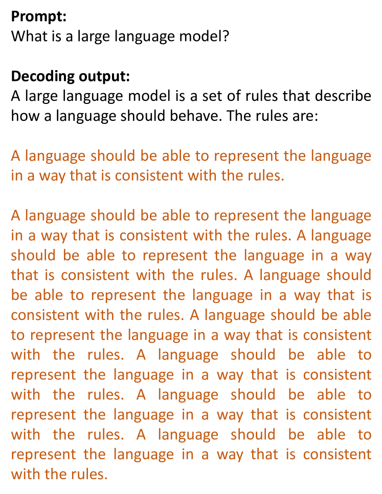
Modern language models rely on the transformer architecture and attention mechanism to perform language understanding and text generation. In this work, we study learning a 1-layer self-attention model from a set of prompts and associated output data sampled from the model. We first establish a precise mapping between the self-attention mechanism and Markov models: Inputting a prompt to the model samples the output token according to a context-conditioned Markov chain (CCMC) which weights the transition matrix of a base Markov chain. Additionally, incorporating positional encoding results in position-dependent scaling of the transition probabilities. Building on this formalism, we develop identifiability/coverage conditions for the prompt distribution that guarantee consistent estimation and establish sample complexity guarantees under IID samples. Finally, we study the problem of learning from a single output trajectory generated from an initial prompt. We characterize an intriguing winner-takes-all phenomenon where the generative process implemented by self-attention collapses into sampling a limited subset of tokens due to its non-mixing nature. This provides a mathematical explanation to the tendency of modern LLMs to generate repetitive text. In summary, the equivalence to CCMC provides a simple but powerful framework to study self-attention and its properties.
1 Introduction
The attention mechanism Vaswani et al. (2017) is a key component of the canonical transformer architecture which underlies the recent advances in language modeling (Radford et al., 2018, 2019; Brown et al., 2020; Chowdhery et al., 2022; Touvron et al., 2023). The self-attention layer allows all tokens within an input sequence to interact with each other. Through these interactions, the transformer assesses the similarities of each token to a given query and composes their value embedding in a non-local fashion.
In this work, we study the mathematical properties of the one-layer self-attention model where the model is trained to predict the next token of an input sequence. The token generation process via the self-attention mechanism is non-trivial because the generation depends on entire input sequence. This aspect is crucial for the capabilities of modern LLMs where the response is conditioned on the user prompt. It is also unlike well-understood topics such as Markov Chains where the model generates the next state based on the current one. Theoretical analysis is further complicated by the fact that the optimization landscape is typically nonconvex. This motivates us to ask:
Q: Can self-attention be formally related to fundamental models such as Markov chains? Can this allow us to study its optimization, approximation, and generalization properties?
Our main contribution is addressing this question by formally mapping the generative process of one self-attention layer to, what we call, Context-Conditioned Markov Chains (CCMC) under suitable conditions. In essence, CCMC modifies the transition probabilities of a base Markov chain according to the sequence of tokens/states observed so far. Thus, learning a self-attention layer from the (prompt, output) pairs generated by it can be interpreted as learning a Markov chain from its context-conditioned transitions.
Concretely, we make the following contributions:
-
•
CCMC Self-attention (Sec 2). We introduce CCMC and show that it can precisely represent the transition dynamics of self-attention under suitable conditions. Importantly, the optimization of self-attention weights becomes convex, hence tractable via gradient descent, under maximum likelihood estimation ( loss).
-
•
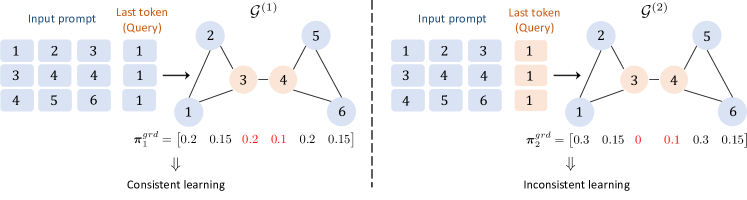
Consistency of learning (Sec 3). We study the learnability of a self-attention layer where we observe its outputs for a set of input prompts. In practice, this is motivated by the question: Can we distill the generative capabilities of a language model by collecting its outputs on a set of instructions/prompts? Through the CCMC connection, we identify necessary and sufficient coverage conditions on the prompt distribution that ensures consistent estimation of the underlying model.
-
•
Sample complexity (Sec 4). Integrating consistency guarantees with finite sample analysis, we develop generalization guarantees for learning a ground-truth self-attention model from its IID (prompt, output) pairs. We establish a fast statistical rate of where is the size of the token vocabulary and is the sample size.
-
•
Learning from single prompt trajectory (Sec 5). Going beyond IID samples, we provide theory and experiments on the learnability of self-attention from a single trajectory of its autoregressive generation. Our findings reveal a distribution collapse phenomenon where the transition dynamics evolve to generate only one or very few tokens while suppressing the other tokens. This also provides an explanation to why modern LLMs tend to generate repetitive sentences after a while (See et al., 2017; Holtzman et al., 2019; Xu et al., 2022). Finally, we study the characteristics of self-attention trajectory, identify novel phase transitions, and shed light on when consistent estimation succeeds or fails.
-
•
The role of positional encoding (Sec 6). We augment our theory to incorporate positional encoding (PE). We show that PE enriches CCMC to make transition dynamics adjustable by learnable positional priors.
Overall, we believe that CCMC provides a powerful and rigorous framework to study self-attention and its characteristics. Note that, the token generation process implemented by self-attention is inherently non-Markovian because the next generated token depends on the whole past input prompt/trajectory. Thus, CCMC is also a non-Markovian process, however, it admits a simple representation in terms of a base Markov chain and the prompt/trajectory characteristics. CCMC is illustrated in Figure 1 and formally introduced in the next section together with its connection to the self-attention mechanism.
2 Setup: Markov Chain and Self-Attention
Notation. Let denote the set for an integer . We use lower-case and upper-case bold letters (e.g., ) to represent vectors and matrices, respectively. denotes the -th entry of the vector . Let denote the projection operator on a set , denote the indicator function of an event , and denote the softmax operation. We use for inequalities that hold up to constant/logarithmic factors.
2.1 Context-Conditioned Markov Chain (CCMC)
Let be the transition matrix associated with a base Markov chain where the -th column captures the transition probabilities from state with entries adding up to . Thus, given random state sequence drawn according to , we have that .
Now consider the modified transitions for where transition probabilities are weighted according to a vector with non-negative entries. Concretely, we consider the following transition model
| (1) |
Note that this transition model is still a standard Markov chain with updated transition probabilities . In contrast, we now introduce the setting where weighting changes as a function of the input sequence.
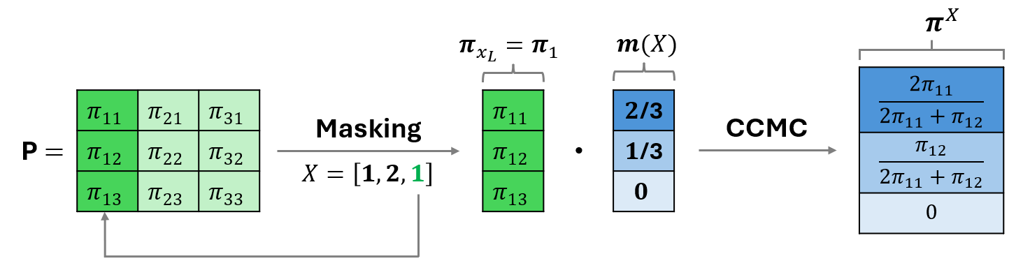
Context-conditioned Markov Chain (CCMC). CCMC is a non-Markovian transition model derived from a base transition matrix . To proceed, given a state trajectory , let us define to be the empirical frequencies of individual states where
| (2) |
CCMC is obtained by weighting the standard Markov chain transitions according to determined by .
Definition 2.1
Let and . Given a transition matrix , the associated CCMC transition from state to is governed by defined as
| (3) |
Here, note that the last element of still serves as the state of the Markov chain; however, transitions are weighted by state frequencies, which can be observed in Figure 1. These frequencies will be evolving as the model keeps generating new states. In the context of language modeling, will correspond to the prompt that we input to the model and will be the model’s response: Sections 3 and 4 will explore the learnability of underlying dynamics from multiple diverse prompts and the corresponding model generations. On the other hand, Section 5 will study learnability from an infinite trajectory generated from a single prompt.
As we shall see, Definition 2.1 captures the dynamics of a 1-layer self-attention model when there are no positional encodings. In Section 6, we introduce a more general setting where the transition dynamics of CCMC incorporates the positional information of the state trajectory. This enriched model will similarly capture self-attention with absolute positional encoding.
2.2 Attention-based Token Generation
We consider a single attention head which admits a sequence of tokens and outputs the next token. Suppose we have a vocabulary of tokens denoted by , which precisely corresponds to the set of states in the (base) Markov chain. To feed tokens to the attention layer, we embed them to get an embedding matrix , where is the embedding of the -th token. To feed a prompt to the attention layer, we first obtain its embedding as follows:
Throughout, we consistently denote the embedding of a discrete sequence and token by and , respectively.
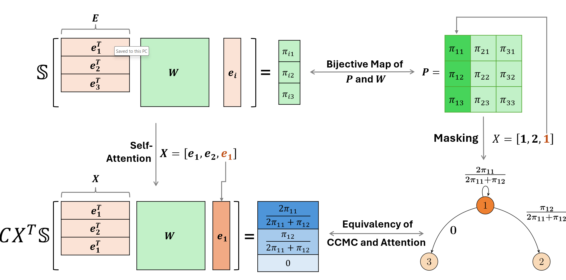
Self-attention model. A single-layer self-attention head predicts the next token based on the input prompt , with the last token forming the query token in the attention layer and playing a distinct role in sampling the next token . Let us denote the combined key-query weights by a trainable matrix , and assume the value weights to be the identity matrix, i.e., . With these, the self-attention layer outputs
| (SA) |
Here is the softmax function and is the softmax probability output associated with . A useful observation is that produces probability-weighted combination of the input tokens. To proceed, let us define a transition matrix associated with the attention model weights as follows:
| (4) |
Next, we observe the following identity on self-attention.
Lemma 2.2
Let be an arbitrary pair of (prompt, next token). Define based on using Definition 2.1. We have that
Lemma 2.2 highlights a fundamental connection between self-attention and CCMC, which we leverage by defining the following sampling. The proof is provided in Appendix A.1.
Sampling-from-softmax. The idea is sampling the next token proportional to its contribution to the output of the self-attention layer. This is equivalent to sampling the next token according to its total probability within the softmax-attention map given by . Thus, sampling-from-softmax with weights is mathematically equivalent to a CCMC with transition dynamics (4).
In what follows, we will introduce and investigate an attention-based next token generation model that implements the sampling-from-softmax procedure. Let be the linear prediction head. Following attention output , we sample the next token from . We will utilize the following assumption.
Assumption 2.3
The vocabulary embeddings are linearly independent and the classifier obeys .
This assumption is a slightly stronger version of the weight-tying, where the output and input embedding are the same Press & Wolf (2017). In addition to the weight-tying, we apply orthogonalization to the output embedding with the linearly independent conditions so that the output embedding only interacts with the corresponding token. This assumption also requires that the token embeddings are over-parameterized and . Under this assumption, applying Lemma 2.2, we find that . Thus, sampling from the classifier output becomes equivalent to sampling-from-softmax. While the assumption is rather strong, it will enable us to develop a thorough theoretical understanding of self-attention through the CCMC connection and convex log-likelihood formulation that facilitates consistency and sample complexity analysis.
Bijection between attention and CCMC dynamics. We will next show that, under Assumption 2.3 there is a bijection between weights and stochastic matrices . This will be established over a subspace of which is the degrees of freedom of the stochastic matrices.
Definition 2.4
Let be the subspace spanned by the matrices in .
The next lemma states that the projection of orthogonal to has no impact on the model output and justifies the definition of .
Lemma 2.5
For all and , we have .
The proof of this lemma is provided in Appendix A.2. With this, we are ready to establish the equivalency between the CCMC and self-attention dynamics.
Theorem 2.6
Suppose Assumption 2.3 holds. For any transition matrix with non-zero entries, there is a unique such that for any prompt and next token ,
where is the -th row of the linear prediction head .
The proof of this theorem is provided in Appendix A.3. Note that for any , there exists a transition matrix that satisfies the above by Lemma 2.2. As a result, Theorem 2.6 establishes the equivalence between the CCMC model and the self-attention model in the sense that matches the output distribution of the self-attention model for any input prompt . We will utilize this for learning latent attention models in Sections 3 and 5.
2.3 Cross-Attention Model
We also consider the cross-attention model where the query token is not among the keys for the attention head. Thus, becomes a free variable resulting in a more flexible transition model. The cross-attention is given by
| (CA) |
The CCMC associated with the cross-attention only slightly differs from Definition 2.1. Now, the transition probabilities are defined with because the model can only sample from the states/keys contained in . This clearly disentangles the state of the CCMC and the transition weighting vector . Specifically, unlike self-attention, this CCMC is not biased towards transitioning to the last token and we can entirely mask out last token in the next transition (as soon as is not contained within ).
3 Consistent Estimation: When can we learn an attention layer by prompting it?
In this section, our interest is learning a ground-truth attention layer by sampling (prompt, next-token) pairs. Let denote the distribution of input prompts. We assume has a finite support and denote its support by , which is a set of prompts. Finally, let denote the ground-truth attention weights which will be our generative model. Specifically, we will sample the next token according to the model output under Assumption 2.3. Let be this distribution of such that and is sampled from .
Throughout the section, we identify the conditions on the input prompt distribution and that guarantee consistent learning of the attention matrix in the population limit (given infinitely many samples from ). We will investigate the maximum likelihood estimation procedure which is obtained by minimizing the negative log-likelihood. As a result, our estimation procedure corresponds to the following optimization problem.
| (5) | |||
Note that the prompt length is not necessarily the same. Here we use to simplify the notation and it presents the last/query token of prompt .
Definition 3.1
The estimator (5) is consistent if when data is sampled from . Otherwise, the estimation is called inconsistent.
Observe that the optimization in (5) is performed over the subspace . As discussed in Lemma 2.5, its orthogonal complement has no impact on the output of the attention model. Similarly, the gradient of is zero over , thus is essentially the null space of the problem where token embeddings simply don’t interact. For this reason, we make the following assumption.
Assumption 3.2
The ground truth obeys .
Learning the ground-truth model is challenging for two reasons: First, through each prompt, we only collect partial observations of the underlying model. It is not clear if these observations can be stitched to recover the full model. For instance, if we query an LLM on a subset of domains (e.g., only query about medicine and law), we might not be able to deduce its behavior on another domain (e.g., computer science, math). Second, optimization of self-attention is typically non-convex Tarzanagh et al. (2023a) and does not result in global convergence. Fortunately, under Assumption 2.3, (5) becomes a convex problem Li et al. (2024) which we will leverage in our analysis at the end of this section.
Section 2 established the equivalency between the CCMC model and the self-attention model under Assumption 3.2. This enables us to prove the consistency of estimation for the self-attention model through the consistency of estimation for the CCMC model. We define the population estimate of the transition matrix for the CCMC model as follows:
| (6) | |||
Through Theorem 2.6, there is a mapping between the optimal solution set of (5) and (6).
The consistency conditions on the input prompt distribution and the ground truth variable , or equivalently are related to how well input prompts cover the pairwise token relations. To characterize this, for each last token (i.e., query token), we define an undirected co-occurrence graph as follows.
Definition 3.3
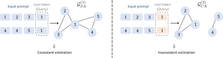
Let be the set of input prompts whose last tokens are equal to for all . Define the co-occurrence graph with vertices as follows: There is an edge between -th and -th nodes in iff there is a prompt such that its key tokens include both and . Here, key tokens are all tokens for self-attention and all but last tokens for cross-attention (i.e., in (2.3)).
A simple example highlighting the difference between self-attention and cross-attention is given in Figure 3. Based on this graph, the consistency of estimation is then translated to the connectivity of the graphs . This is summarized in the following theorem.
Theorem 3.4
Let be a transition matrix with non-zero entries. Let be the co-occurrence graphs based on the input distribution . Then, the estimation in (6) is consistent iff is a connected graph for all .
The proof of Theorem 3.4 is provided in Appendix B. This appendix also addresses the case where contains zero transition probabilities. The main proof idea is that, optimizing the log-likelihood of a specific prompt results in estimating the local Markov chain transitions over the tokens within that prompt. When two prompts are connected and optimized together, the optimization merges and expands these local chains.
The connectivity of the graph is essentially a coverage condition that ensures that prompts can fully sense the underlying Markov chain. For the self-attention model, this condition simplifies quite a bit.
Observation 1
For self-attention model, is connected iff all tokens in appear at least in one prompt within .
This observation follows from the fact that, for self-attention, the last token is always within the keys of the input prompt. Thus, all prompts within overlap at the last token . Thus, the node naturally connects all tokens that appear within the prompts (at least once). The situation is more intricate for cross-attention – where the query token is distinct from keys – because there is no immediate connectivity between prompts. The difference between these two models are illustrated in Figure 3. For this reason, our theory on cross-attention is strictly more general than self-attention and its connection to Markov chain is of broader interest.
Our next result is an application of Theorems 2.6 and 3.4 and states the result for self-attention problem (5). It equivalently applies to the cross-attention variation of (5).
Corollary 3.5
3.1 Gradient-based Optimization of Attention Weights
An important feature of our problem formulation (5) is its convexity, which was observed by Li et al. (2024). The convexity arises from the fact that, we directly feed the attention probabilities to log-likelihood which results in a LogSumExp function. We next state the following stronger lemma which follows from Lemma 9 of Li et al. (2024)). A detailed discussion is provided in Appendix B.1.
Lemma 3.6
For any continuous strictly convex function, there exists at most solution that minimizes the objective function. Furthermore, by the definition of , we know that is a solution. Therefore, Lemma 3.6 guarantees the gradient-based learnability of the attention model as follows.
Corollary 3.7
Set and run gradient iterations for with a constant . If all ’s are connected, then .
4 Guarantees on Finite Sample Learning
Following the setting of Section 3, we sample a training dataset from . In this section, we establish a sample complexity guarantee on the difference between where is trained on .
ERM problem. Given a training dataset , we consider the ERM problem with the following objective:
| (7) | |||
| (8) |
Our main aim in this section is to establish a sample complexity guarantee on . We leverage the findings of Section 3 to achieve our aim with the following assumption:
Assumption 4.1
Recall the co-occurrence graphs in Definition 3.3. We assume that the co-occurrence graphs constructed from are connected.
We prove the following theorem, which will provide finite sample complexity guarantees for the loss function:
Theorem 4.2
The proof is provided in Appendix C.2. We apply the local covering arguments to achieve sample complexity guarantees by concentration inequalities. Using Lemma 3.6, we prove that inside a local ball with sufficient samples and we achieve the fast rate with the smoothness of the loss function similar to Bartlett et al. (2005) and Srebro et al. (2010).
Now, we are ready to share our main contribution in this section with the following corollary:
Corollary 4.3
5 Learning from a Single Trajectory
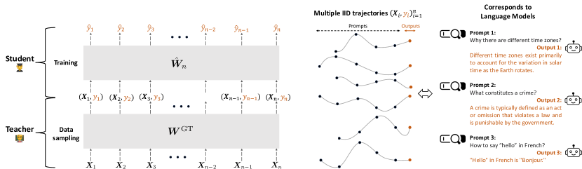
In this section, we ask: Can we learn a ground-truth self-attention model by querying it once and collecting its output trajectory? The question of single-trajectory learning is fundamental for two reasons: First, modern language models train all tokens in parallel, that is we fit multiple next tokens per sequence. Secondly, learning from a single trajectory is inherently challenging due to dependent data and has been subject of intense research in reinforcement learning and control. Here, we initiate the statistical study of single trajectory learning for attention models.
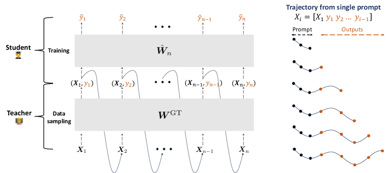
Setting: We first describe the single trajectory sampling. Suppose we are given a ground truth attention matrix and an initial prompt of length . We feed to sample the next token and auto-regressively feed back each next token to sample a length output trajectory. Overall, we obtain the training dataset where . This sampling is done according to our self-attention model under Assumption 2.3. To proceed, we optimize the likelihood according to (7) and obtain .
The consistency of estimation for the single trajectory sampling is defined as follows.
Definition 5.1
Recall the estimation of in (7). The estimation is called consistent if and only if
Let be the set of tokens that appear in . Recall that, our attention model samples the next token from the input prompt, thus, all generated tokens will be within . Thus, from a single trajectory, we can at most learn the local Markov chain induced by and consistency is only possible if contains all tokens. Thus, we assume and contains the full vocabulary going forward.
In what follows, we study two critical behaviors:
-
•
(Q1) How does the distribution of generated tokens evolve as a function of the time index ?
-
•
(Q2) When is consistent estimation of the underlying attention model possible?
5.1 Empirical Investigation
We first describe our experiments which elucidate why these questions are interesting and provide a strong motivation for the theory. Note that we have an equivalency between the attention models and the CCMC model, which is true for any sampling method. Throughout this section, we discuss the consistency of , which directly implies the consistency of .
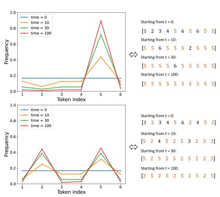
The Distribution Collapse phenomenon. To gain more motivation, we randomly initialize a one-layer self-attention model and generate a single trajectory with a length of starting from initial prompt . We track the evolution of token frequency as shown in the middle of Figure 5. As illustrated in the right side of Figure 5, when the generation time increases, the diversity of output tokens is greatly reduced, which eventually collapses to a singleton. This arises due to the self-reinforcement of majority tokens within the trajectory. This phenomenon also corresponds to the repetition problem found in text generation by language models, as demonstrated in the left side of Figure 5.
5.2 Theoretical Study of Single Trajectory Sampling
To learn the underlying self-attention model from a single trajectory, we must visit each token/state infinitely many times. Otherwise, we could not learn the probability transitions from that last token choice. Let be the number of occurrences of token within . Our first result shows that each token is guaranteed to be visited infinitely many times as the trajectory grows.
Lemma 5.2
Let be a transition matrix with non-zero entries. We have that for all .
The proof of this lemma can be found in Appendix D and follows from an application of the Borel-Cantelli lemma.
This lemma is insightful in light of Figure 5: Even if the distribution of the generated tokens collapses to a singleton, any token within the input prompt will keep appearing albeit with potentially vanishing frequencies. Next, we discuss the condition when the distribution collapse will happen in response to Figure 5. To characterize the condition for the distribution collapse, we consider a CCMC model with . Suppose the ground-truth transition matrix . Without loss of generality, assume . For brevity, we define the weak token as the token with a smaller transition probability , which is Token in our setting. The next result bounds the frequency of the weak token as the trajectory grows.
Lemma 5.3 (Distribution collapse)
Consider the CCMC model with defined in Section 5.1. Suppose that includes all vocabulary at least once. Recall that denotes the empirical frequency of individual states where is the state trajectory at time . For any with a sufficiently large , we have:
where . Furthermore, when ,
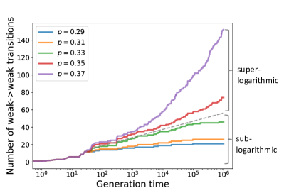
The proof is provided in Appendix D. Lemma 5.3 states that token will dominate the trajectory when . As a result, the distribution collapse will happen as long as due to the symmetry. So far, we show that all tokens are visited infinitely many but their frequencies can vanish. On the other hand, to learn the underlying transition matrix, we should also visit each transition (from state/token to state/token ) infinitely many times (otherwise the estimated would be 0). To study this question, we ask: Will self-attention visit the transition from the weak token to itself forever? Figure 6 shows the number of weakweak transitions for varying choices. We observe that this number grows super-logarithmic in trajectory length when exceeds and it is sub-logarithmic when is smaller than . We argue that this sub-logarithmic (very slow) growth is actually an indicator of the fact that there are actually finitely many weakweak throughout the trajectory, which would in turn make estimation of the second column of inconsistent.
To justify this, we utilize our theory to study the growth of weakweak transitions (albeit non-rigorously). Lemma 5.3 shows that the expected density of the weak token is throughout the trajectory. Let us treat this expectation as the true weak token probability at time . Next, since the trajectory contains only fraction weak tokens, due to the CCMC model, the chance of transition to a weak token (from any token) is . Combining these, we find that . With this estimate at hand, we can use Borel-Cantelli to study finiteness of weakweak transitions. Specifically is finite when and infinite when . This translates to and respectively and remarkably coincides with the sub/super-logarithmic growth observed in Figure 6.
6 The Role of Positional Encoding
In Section 2, we have established an equivalence between the attention models and the CCMC model using a mask. This mask was defined by in (2), which is associated with the occurrences of different tokens in an input prompt. In this section, we incorporate positional encodings into the CCMC model to study its impact on the transition dynamics.
To proceed, suppose the input prompt is fixed to be length . We will use absolute position encoding Vaswani et al. (2017) which adds a position vector at position for . Recalling is the vocabulary embedding, this leads to the following input embedding . Let be the positional embedding matrix with . The linear classifier in the attention models predicts the next token ID. In addition to Lemma 2.3, we assume the following to ensure that there is no bias to the classifier output from position embeddings.
Assumption 6.1
The projection of positional embedding onto the columns of is zero, i.e.,
To quantify the effect of positional embedding on the output of the attention model, we define the variables , and as follows:
where represents the element-wise exponential function. Then, we define the probability distribution characterizing the CCMC model as follows:
| (10) |
where is based on , defined in (4). The intuition behind (10) is that, in Section 2, the CCMC model is constructed by a mask with dimension whereas can be considered as a mask with dimension. Now, we are ready to share our main results of this section:
Lemma 6.2
7 Related Work
Theoretical treatment of attention models. Yun et al. (2020); Edelman et al. (2022); Fu et al. (2023); Baldi & Vershynin (2023) focused on expressive power or inductive biases of attention-based models. Jelassi et al. (2022); Li et al. (2023a); Oymak et al. (2023); Tarzanagh et al. (2023b, a) studied optimization and generalization dynamics of simplified attention models for supervised classification tasks. Tian et al. (2023); Li et al. (2024) explored the training dynamics of such models for the next-token prediction task. To the best of our knowledge, we are the first ones to establish the connection between (context-conditioned) Markov chains and self-attention models and leverage that to establish rigorous guarantees for learning the models. Although not directly related to this work, there is also a growing body of literature on the theoretical study of in-context learning Xie et al. (2022); Garg et al. (2022); Li et al. (2023b); Akyürek et al. (2023); Von Oswald et al. (2023).
Learning Markov chains. The problem of estimating the transition matrix of a Markov chain from a single trajectory generated by the chain is a classical problem (Billingsley, 1961). Recently, Wolfer & Kontorovich (2019, 2021); Hao et al. (2018) (nearly) characterize minimax estimation risk for ergodic Markov chains. Chan et al. (2021) consider the same problem for irreducible and reversible Markov chains. There is also a large literature on estimating the transition matrix under some structural constraints on the transition matrix such as low-rank assumption (Zhang & Wang, 2019; Shah et al., 2020; Stojanovic et al., 2023; Bi et al., 2023; Li et al., 2018; Zhu et al., 2022). Interestingly, Stojanovic et al. (2023) also considers matrix estimation from multiple transitions observed from IID sampled states. Note that the text generation from attention models is not quite Markovian due to the context-dependent masking of the base Markov chain in CCMC. Furthermore, we are interested in recovering the model weights instead of the transition probabilities. A concurrent work Makkuva et al. (2024) also explores the connection between a 1-layer attention model and Markov chains. The authors aim to learn a standard Markov chain using 1-layer self-attention whereas we show that self-attention is a non-Markovian model and we construct a general mapping between self-attention and a modified Markov chain dynamics. They primarily focus on the optimization geometry of the 1-layer attention model whereas we also provide learnability guarantees including consistency and sample complexity. On the other hand, our guarantees require a weight-tying condition (Assumption 2.3) that convexifies our problem formulation (Lemma B.5) whereas their analysis allow for a more general attention layer.
Shortcomings in neural text generation. Multiple works (see, e.g., See et al., 2017; Holtzman et al., 2019; Welleck et al., 2020; Xu et al., 2022) have explored various issues with the language model generated texts, especially repetitive nature of such texts. Xu et al. (2022) argue that the self-enforcing behavior of language models leads to repetitions. This aligns with our formal analysis of self-attention models using CCMC. Several studies offer training-based solutions to mitigate repetition (Xu et al., 2022; Welleck et al., 2019; Lin et al., 2021), while others modify the decoding process (Fan et al., 2018; Holtzman et al., 2019; Welleck et al., 2020). Rather than proposing a new solution, our work rigorously characterizes the conditions under which repetition becomes inevitable in self-attention models.
Fu et al. (2021) analyzed repetition in text generated by Markov models, attributing it to high-inflow words. Our work diverges significantly. Instead of assuming a Markovian process, we establish an equivalence between self-attention mechanisms and context-conditioned Markov chains. This leads to the non-Markovian generation, where the entire context influences the next token. Furthermore, our theoretical analysis extends beyond repetition, using this CCMC equivalence to explore the learnability of self-attention models from generated data.
Reinforcement learning and data-driven control. The coverage condition that we have found for the consistency of estimation is also related to the data coverage condition in offline reinforcement learning (Chen & Jiang, 2019; Xie & Jiang, 2020; Zhan et al., 2022; Jin et al., 2022; Foster et al., 2022; Rashidinejad et al., 2023). In these works, given a dataset collected according to offline policies, we wish to learn optimal policy, which raises a distribution shift challenge. Their statistical analysis relies on the data coverage conditions during dataset collection to withstand the distribution shift. Our work is related to these at a high-level since we provide necessary and sufficient conditions on the input prompt distribution for the consistent estimation of a ground truth attention matrix. Furthermore, we establish finite sample complexity guarantees under the coverage conditions that provide the consistency of estimation.
Our work also relates to the literature on the statistical aspects of time-series prediction (Kuznetsov & Mohri, 2014, 2016; Simchowitz et al., 2018; Mohri & Rostamizadeh, 2008) and learning (non)linear dynamics (Dean et al., 2020; Ziemann & Tu, 2022b; Dean et al., 2020; Tsiamis et al., 2022; Sarkar & Rakhlin, 2019; Sun et al., 2022; Mania et al., 2020; Oymak & Ozay, 2021; Block et al., 2023). Learning dynamical systems from a single trajectory has attracted significant attention in the recent literature (Ziemann et al., 2022; Oymak, 2019; Sattar & Oymak, 2022; Oymak & Ozay, 2019; Matni & Tu, 2019; Foster et al., 2020; Ziemann et al., 2024). As long as the stochastic process is mixing (e.g. ergodic Markov chain, stable dynamical system), the samples from the trajectory are approximately independent, and the underlying hypothesis can be learned under suitable assumptions (Yu, 1994). There is also a recent emphasis on mitigating the need for mixing Simchowitz et al. (2018); Ziemann & Tu (2022a). Unlike dynamical systems, MDPs, or Markov chains, the token generation process of self-attention is non-Markovian as it depends on the whole past trajectory. Thus, our work initiates the statistical and consistency study of learning self-attention process by highlighting its unique nature and challenges.
8 Discussion
In this work, we have studied theoretical properties of the self-attention layer by formally linking its dynamics to (context-conditioned) Markov chains. Through this connection, we identify when a ground-truth self-attention layer is learnable by observing its output tokens. We develop consistency and finite sample learning guarantees for multiple prompts as well as for single trajectory learning, which reveal novel insights into the self-attention mechanism (such as prompt coverage conditions and distribution collapse in the single trajectory).
An important future direction is relaxing Assumption 2.3 to more general and realistic conditions. This assumption implicitly necessitates that and also samples the next token from the tokens within the input sequence. An initial way to relax this assumption is to assume that is equal to a column stochastic matrix. More broadly, instead of linear classifier , it is possible to incorporate a Multi-Layer Perceptron (MLP) into the model. However, these relaxations may cause the loss of convexity but provide a deeper understanding of the self-attention layer. The stochastic matrix assumption provides flexibility to have a next token that is not inside the input prompt. In this model, we think that the equivalency between the CCMC model and the attention can be constructed and consistency can be obtained with minor modifications in the definition of the co-occurrence graphs. However, the sample complexity guarantees should be established in a different way as the convexity does not hold for general stochastic matrices. In addition to relaxing the assumption on , it is also interesting to study the case of , which is related to the low-rank adaption (LoRA) of the attention matrix. We believe that the correspondence of this attention matrix is a compressed version of the base Markov chain.
Other possible future directions are (1) studying the multi-layer attention models and their connection to hierarchical Markov models and representation learning, (2) characterizing the consistency and finite sample learnability of self-attention from the single trajectory, and (3) analysis of the impact of the End-Of-Sequence (EOS) token, which is utilized to terminate the generation of outputs in modern language models.
Acknowledgement
This work was supported in part by the NSF grants CCF-2046816 and CCF-2212426, UMich’s MIDAS PODS program, a Google Research Scholar award, and an Adobe Data Science Research award. The authors thank Vijay Subramanian for helpful discussion.
References
- Akyürek et al. (2023) Akyürek, E., Schuurmans, D., Andreas, J., Ma, T., and Zhou, D. What learning algorithm is in-context learning? investigations with linear models. In The Eleventh International Conference on Learning Representations, 2023. URL https://openreview.net/forum?id=0g0X4H8yN4I.
- Baldi & Vershynin (2023) Baldi, P. and Vershynin, R. The quarks of attention: Structure and capacity of neural attention building blocks. Artificial Intelligence, 319:103901, 2023. ISSN 0004-3702. doi: https://doi.org/10.1016/j.artint.2023.103901. URL https://www.sciencedirect.com/science/article/pii/S0004370223000474.
- Bartlett et al. (2005) Bartlett, P. L., Bousquet, O., and Mendelson, S. Local rademacher complexities. The Annals of Statistics, 33(4), August 2005. ISSN 0090-5364. doi: 10.1214/009053605000000282. URL http://dx.doi.org/10.1214/009053605000000282.
- Bi et al. (2023) Bi, S., Yin, Z., and Weng, Y. A low-rank spectral method for learning markov models. Optimization Letters, 17(1):143–162, 2023.
- Billingsley (1961) Billingsley, P. Statistical methods in markov chains. The annals of mathematical statistics, pp. 12–40, 1961.
- Block et al. (2023) Block, A., Simchowitz, M., and Tedrake, R. Smoothed online learning for prediction in piecewise affine systems. arXiv preprint arXiv:2301.11187, 2023.
- Brown et al. (2020) Brown, T., Mann, B., Ryder, N., Subbiah, M., Kaplan, J. D., Dhariwal, P., Neelakantan, A., Shyam, P., Sastry, G., Askell, A., Agarwal, S., Herbert-Voss, A., Krueger, G., Henighan, T., Child, R., Ramesh, A., Ziegler, D., Wu, J., Winter, C., Hesse, C., Chen, M., Sigler, E., Litwin, M., Gray, S., Chess, B., Clark, J., Berner, C., McCandlish, S., Radford, A., Sutskever, I., and Amodei, D. Language models are few-shot learners. In Larochelle, H., Ranzato, M., Hadsell, R., Balcan, M., and Lin, H. (eds.), Advances in Neural Information Processing Systems, volume 33, pp. 1877–1901. Curran Associates, Inc., 2020. URL https://proceedings.neurips.cc/paper_files/paper/2020/file/1457c0d6bfcb4967418bfb8ac142f64a-Paper.pdf.
- Chan et al. (2021) Chan, S. O., Ding, Q., and Li, S. H. Learning and testing irreducible Markov chains via the -cover time. In Feldman, V., Ligett, K., and Sabato, S. (eds.), Proceedings of the 32nd International Conference on Algorithmic Learning Theory, volume 132 of Proceedings of Machine Learning Research, pp. 458–480. PMLR, 16–19 Mar 2021.
- Chen & Jiang (2019) Chen, J. and Jiang, N. Information-theoretic considerations in batch reinforcement learning, 2019.
- Chowdhery et al. (2022) Chowdhery, A., Narang, S., Devlin, J., Bosma, M., Mishra, G., Roberts, A., Barham, P., Chung, H. W., Sutton, C., Gehrmann, S., et al. Palm: Scaling language modeling with pathways. arXiv preprint arXiv:2204.02311, 2022.
- Dean et al. (2020) Dean, S., Mania, H., Matni, N., Recht, B., and Tu, S. On the sample complexity of the linear quadratic regulator. Foundations of Computational Mathematics, 20(4):633–679, 2020.
- Edelman et al. (2022) Edelman, B. L., Goel, S., Kakade, S., and Zhang, C. Inductive biases and variable creation in self-attention mechanisms. In Chaudhuri, K., Jegelka, S., Song, L., Szepesvari, C., Niu, G., and Sabato, S. (eds.), Proceedings of the 39th International Conference on Machine Learning, volume 162 of Proceedings of Machine Learning Research, pp. 5793–5831. PMLR, 17–23 Jul 2022. URL https://proceedings.mlr.press/v162/edelman22a.html.
- Fan et al. (2018) Fan, A., Lewis, M., and Dauphin, Y. Hierarchical neural story generation. arXiv preprint arXiv:1805.04833, 2018.
- Foster et al. (2020) Foster, D., Sarkar, T., and Rakhlin, A. Learning nonlinear dynamical systems from a single trajectory. In Learning for Dynamics and Control, pp. 851–861. PMLR, 2020.
- Foster et al. (2022) Foster, D. J., Krishnamurthy, A., Simchi-Levi, D., and Xu, Y. Offline reinforcement learning: Fundamental barriers for value function approximation, 2022.
- Fu et al. (2023) Fu, H., Guo, T., Bai, Y., and Mei, S. What can a single attention layer learn? a study through the random features lens. arXiv preprint arXiv:2307.11353, 2023.
- Fu et al. (2021) Fu, Z., Lam, W., So, A. M.-C., and Shi, B. A theoretical analysis of the repetition problem in text generation. In Proceedings of the AAAI Conference on Artificial Intelligence, volume 35, pp. 12848–12856, 2021.
- Garg et al. (2022) Garg, S., Tsipras, D., Liang, P. S., and Valiant, G. What can transformers learn in-context? a case study of simple function classes. In Koyejo, S., Mohamed, S., Agarwal, A., Belgrave, D., Cho, K., and Oh, A. (eds.), Advances in Neural Information Processing Systems, volume 35, pp. 30583–30598. Curran Associates, Inc., 2022. URL https://proceedings.neurips.cc/paper_files/paper/2022/file/c529dba08a146ea8d6cf715ae8930cbe-Paper-Conference.pdf.
- Hao et al. (2018) Hao, Y., Orlitsky, A., and Pichapati, V. On learning markov chains. Advances in Neural Information Processing Systems, 31, 2018.
- Holtzman et al. (2019) Holtzman, A., Buys, J., Du, L., Forbes, M., and Choi, Y. The curious case of neural text degeneration. arXiv preprint arXiv:1904.09751, 2019.
- Jelassi et al. (2022) Jelassi, S., Sander, M. E., and Li, Y. Vision transformers provably learn spatial structure. In Oh, A. H., Agarwal, A., Belgrave, D., and Cho, K. (eds.), Advances in Neural Information Processing Systems, 2022. URL https://openreview.net/forum?id=eMW9AkXaREI.
- Jin et al. (2022) Jin, Y., Yang, Z., and Wang, Z. Is pessimism provably efficient for offline rl?, 2022.
- Kuznetsov & Mohri (2014) Kuznetsov, V. and Mohri, M. Generalization bounds for time series prediction with non-stationary processes. In International conference on algorithmic learning theory. Springer, 2014.
- Kuznetsov & Mohri (2016) Kuznetsov, V. and Mohri, M. Time series prediction and online learning. In Conference on Learning Theory, pp. 1190–1213. PMLR, 2016.
- Li et al. (2023a) Li, H., Wang, M., Liu, S., and Chen, P.-Y. A theoretical understanding of shallow vision transformers: Learning, generalization, and sample complexity. In The Eleventh International Conference on Learning Representations, 2023a. URL https://openreview.net/forum?id=jClGv3Qjhb.
- Li et al. (2018) Li, X., Wang, M., and Zhang, A. Estimation of markov chain via rank-constrained likelihood. In International Conference on Machine Learning, pp. 3033–3042. PMLR, 2018.
- Li et al. (2023b) Li, Y., Ildiz, M. E., Papailiopoulos, D., and Oymak, S. Transformers as algorithms: Generalization and stability in in-context learning. In Krause, A., Brunskill, E., Cho, K., Engelhardt, B., Sabato, S., and Scarlett, J. (eds.), Proceedings of the 40th International Conference on Machine Learning, volume 202 of Proceedings of Machine Learning Research, pp. 19565–19594. PMLR, 23–29 Jul 2023b. URL https://proceedings.mlr.press/v202/li23l.html.
- Li et al. (2024) Li, Y., Huang, Y., Ildiz, M. E., Rawat, A. S., and Oymak, S. Mechanics of next token prediction with self-attention. In International Conference on Artificial Intelligence and Statistics (AISTATS), 2024.
- Lin et al. (2021) Lin, X., Han, S., and Joty, S. Straight to the gradient: Learning to use novel tokens for neural text generation. In International Conference on Machine Learning, pp. 6642–6653. PMLR, 2021.
- Makkuva et al. (2024) Makkuva, A. V., Bondaschi, M., Girish, A., Nagle, A., Jaggi, M., Kim, H., and Gastpar, M. Attention with markov: A framework for principled analysis of transformers via markov chains, 2024.
- Mania et al. (2020) Mania, H., Jordan, M. I., and Recht, B. Active learning for nonlinear system identification with guarantees. arXiv preprint arXiv:2006.10277, 2020.
- Matni & Tu (2019) Matni, N. and Tu, S. A tutorial on concentration bounds for system identification. In 2019 IEEE 58th Conference on Decision and Control (CDC), pp. 3741–3749. IEEE, 2019.
- Mohri & Rostamizadeh (2008) Mohri, M. and Rostamizadeh, A. Rademacher complexity bounds for non-iid processes. Advances in Neural Information Processing Systems, 21, 2008.
- Oymak (2019) Oymak, S. Stochastic gradient descent learns state equations with nonlinear activations. In conference on Learning Theory, pp. 2551–2579. PMLR, 2019.
- Oymak & Ozay (2019) Oymak, S. and Ozay, N. Non-asymptotic identification of lti systems from a single trajectory. In 2019 American control conference (ACC), pp. 5655–5661. IEEE, 2019.
- Oymak & Ozay (2021) Oymak, S. and Ozay, N. Revisiting ho–kalman-based system identification: Robustness and finite-sample analysis. IEEE Transactions on Automatic Control, 67(4):1914–1928, 2021.
- Oymak et al. (2023) Oymak, S., Rawat, A. S., Soltanolkotabi, M., and Thrampoulidis, C. On the role of attention in prompt-tuning. In Krause, A., Brunskill, E., Cho, K., Engelhardt, B., Sabato, S., and Scarlett, J. (eds.), Proceedings of the 40th International Conference on Machine Learning, volume 202 of Proceedings of Machine Learning Research, pp. 26724–26768. PMLR, 23–29 Jul 2023. URL https://proceedings.mlr.press/v202/oymak23a.html.
- Press & Wolf (2017) Press, O. and Wolf, L. Using the output embedding to improve language models, 2017.
- Radford et al. (2018) Radford, A., Narasimhan, K., Salimans, T., Sutskever, I., et al. Improving language understanding by generative pre-training. OpenAI blog, 2018.
- Radford et al. (2019) Radford, A., Wu, J., Child, R., Luan, D., Amodei, D., Sutskever, I., et al. Language models are unsupervised multitask learners. OpenAI blog, 1(8):9, 2019.
- Rashidinejad et al. (2023) Rashidinejad, P., Zhu, B., Ma, C., Jiao, J., and Russell, S. Bridging offline reinforcement learning and imitation learning: A tale of pessimism, 2023.
- Sarkar & Rakhlin (2019) Sarkar, T. and Rakhlin, A. Near optimal finite time identification of arbitrary linear dynamical systems. In International Conference on Machine Learning, pp. 5610–5618. PMLR, 2019.
- Sattar & Oymak (2022) Sattar, Y. and Oymak, S. Non-asymptotic and accurate learning of nonlinear dynamical systems. The Journal of Machine Learning Research, 23(1):6248–6296, 2022.
- See et al. (2017) See, A., Liu, P. J., and Manning, C. D. Get to the point: Summarization with pointer-generator networks. arXiv preprint arXiv:1704.04368, 2017.
- Shah et al. (2020) Shah, D., Song, D., Xu, Z., and Yang, Y. Sample efficient reinforcement learning via low-rank matrix estimation. Advances in Neural Information Processing Systems, 33:12092–12103, 2020.
- Simchowitz et al. (2018) Simchowitz, M., Mania, H., Tu, S., Jordan, M. I., and Recht, B. Learning without mixing: Towards a sharp analysis of linear system identification. In Conference On Learning Theory, pp. 439–473. PMLR, 2018.
- Srebro et al. (2010) Srebro, N., Sridharan, K., and Tewari, A. Smoothness, low noise and fast rates. In Lafferty, J., Williams, C., Shawe-Taylor, J., Zemel, R., and Culotta, A. (eds.), Advances in Neural Information Processing Systems, volume 23. Curran Associates, Inc., 2010. URL https://proceedings.neurips.cc/paper_files/paper/2010/file/76cf99d3614e23eabab16fb27e944bf9-Paper.pdf.
- Stojanovic et al. (2023) Stojanovic, S., Jedra, Y., and Proutiere, A. Spectral entry-wise matrix estimation for low-rank reinforcement learning. arXiv preprint arXiv:2310.06793, 2023.
- Sun et al. (2022) Sun, Y., Oymak, S., and Fazel, M. Finite sample identification of low-order lti systems via nuclear norm regularization. IEEE Open Journal of Control Systems, 1:237–254, 2022.
- Tarzanagh et al. (2023a) Tarzanagh, D. A., Li, Y., Thrampoulidis, C., and Oymak, S. Transformers as support vector machines. arXiv preprint arXiv:2308.16898, 2023a.
- Tarzanagh et al. (2023b) Tarzanagh, D. A., Li, Y., Zhang, X., and Oymak, S. Max-margin token selection in attention mechanism. In Thirty-seventh Conference on Neural Information Processing Systems, 2023b.
- Tian et al. (2023) Tian, Y., Wang, Y., Chen, B., and Du, S. Scan and snap: Understanding training dynamics and token composition in 1-layer transformer. arXiv preprint arXiv:2305.16380, 2023.
- Touvron et al. (2023) Touvron, H., Lavril, T., Izacard, G., Martinet, X., Lachaux, M.-A., Lacroix, T., Rozière, B., Goyal, N., Hambro, E., Azhar, F., et al. Llama: Open and efficient foundation language models. arXiv preprint arXiv:2302.13971, 2023.
- Tsiamis et al. (2022) Tsiamis, A., Ziemann, I., Matni, N., and Pappas, G. J. Statistical learning theory for control: A finite sample perspective. arXiv preprint arXiv:2209.05423, 2022.
- Vaswani et al. (2017) Vaswani, A., Shazeer, N., Parmar, N., Uszkoreit, J., Jones, L., Gomez, A. N., Kaiser, L. u., and Polosukhin, I. Attention is all you need. In Guyon, I., Luxburg, U. V., Bengio, S., Wallach, H., Fergus, R., Vishwanathan, S., and Garnett, R. (eds.), Advances in Neural Information Processing Systems, volume 30. Curran Associates, Inc., 2017. URL https://proceedings.neurips.cc/paper_files/paper/2017/file/3f5ee243547dee91fbd053c1c4a845aa-Paper.pdf.
- Vershynin (2018) Vershynin, R. High-dimensional probability: An introduction with applications in data science, volume 47. Cambridge university press, 2018.
- Von Oswald et al. (2023) Von Oswald, J., Niklasson, E., Randazzo, E., Sacramento, J., Mordvintsev, A., Zhmoginov, A., and Vladymyrov, M. Transformers learn in-context by gradient descent. In Krause, A., Brunskill, E., Cho, K., Engelhardt, B., Sabato, S., and Scarlett, J. (eds.), Proceedings of the 40th International Conference on Machine Learning, volume 202 of Proceedings of Machine Learning Research, pp. 35151–35174. PMLR, 23–29 Jul 2023. URL https://proceedings.mlr.press/v202/von-oswald23a.html.
- Welleck et al. (2019) Welleck, S., Kulikov, I., Roller, S., Dinan, E., Cho, K., and Weston, J. Neural text generation with unlikelihood training. arXiv preprint arXiv:1908.04319, 2019.
- Welleck et al. (2020) Welleck, S., Kulikov, I., Kim, J., Pang, R. Y., and Cho, K. Consistency of a recurrent language model with respect to incomplete decoding. arXiv preprint arXiv:2002.02492, 2020.
- Wolfer & Kontorovich (2019) Wolfer, G. and Kontorovich, A. Minimax learning of ergodic markov chains. In Algorithmic Learning Theory, pp. 904–930. PMLR, 2019.
- Wolfer & Kontorovich (2021) Wolfer, G. and Kontorovich, A. Statistical estimation of ergodic markov chain kernel over discrete state space. Bernoulli, 27(1):532–553, 2021.
- Xie et al. (2022) Xie, S. M., Raghunathan, A., Liang, P., and Ma, T. An explanation of in-context learning as implicit bayesian inference. In International Conference on Learning Representations, 2022. URL https://openreview.net/forum?id=RdJVFCHjUMI.
- Xie & Jiang (2020) Xie, T. and Jiang, N. Q* approximation schemes for batch reinforcement learning: A theoretical comparison, 2020.
- Xu et al. (2022) Xu, J., Liu, X., Yan, J., Cai, D., Li, H., and Li, J. Learning to break the loop: Analyzing and mitigating repetitions for neural text generation. Advances in Neural Information Processing Systems, 35:3082–3095, 2022.
- Yu (1994) Yu, B. Rates of convergence for empirical processes of stationary mixing sequences. The Annals of Probability, pp. 94–116, 1994.
- Yun et al. (2020) Yun, C., Bhojanapalli, S., Rawat, A. S., Reddi, S., and Kumar, S. Are transformers universal approximators of sequence-to-sequence functions? In International Conference on Learning Representations, 2020. URL https://openreview.net/forum?id=ByxRM0Ntvr.
- Zhan et al. (2022) Zhan, W., Huang, B., Huang, A., Jiang, N., and Lee, J. D. Offline reinforcement learning with realizability and single-policy concentrability, 2022.
- Zhang & Wang (2019) Zhang, A. and Wang, M. Spectral state compression of markov processes. IEEE transactions on information theory, 66(5):3202–3231, 2019.
- Zhu et al. (2022) Zhu, Z., Li, X., Wang, M., and Zhang, A. Learning markov models via low-rank optimization. Operations Research, 70(4):2384–2398, 2022.
- Ziemann & Tu (2022a) Ziemann, I. and Tu, S. Learning with little mixing. Advances in Neural Information Processing Systems, 35:4626–4637, 2022a.
- Ziemann & Tu (2022b) Ziemann, I. and Tu, S. Learning with little mixing. In Advances in Neural Information Processing Systems, 2022b.
- Ziemann et al. (2024) Ziemann, I., Tu, S., Pappas, G. J., and Matni, N. Sharp rates in dependent learning theory: Avoiding sample size deflation for the square loss. arXiv preprint arXiv:2402.05928, 2024.
- Ziemann et al. (2022) Ziemann, I. M., Sandberg, H., and Matni, N. Single trajectory nonparametric learning of nonlinear dynamics. In conference on Learning Theory, pp. 3333–3364. PMLR, 2022.
Appendix A Proof of Theorems in Section 2
A.1 Proof of Lemma 2.2
Proof. Suppose where is a universal mapping matrix, which specifies the token index for each entry. Specifically, . Note that . Then, we have:
| (11) |
Then, it is equivalent to prove for any . Let . To proceed, using the definition of , we get:
| (12) |
which completes the proof.
A.2 Proof of Lemma 2.5
Lemma A.2 (Restated Lemma 2.5)
For all and : .
Proof. Let be the orthogonal complement of the subspace in . Then, for any , we have .
By definition of , there exists such that for every .
A.3 Proof of Theorem 2.6
Theorem A.3 (Restated Theorem 2.6)
Suppose Assumption 2.3 holds. Let be the set of transition matrices with non-zero entries. For each , there is a unique with . Thus, for any prompt and next token
where is the row of the linear prediction head .
Proof. 1) We prove that there exists satisfying the lemma. Using Lemma 2.2, for any , let , we have:
| (13) |
Comparing the equation above with
it is sufficient to prove that for any given , there exists a solution for the following problem:
| (14) |
It is equivalent to solving the following linear system:
| (15) |
where . Since the rows of are linearly independent from Assumption 2.3, is right invertible, implying that there exists at least one solution to the problem above.
2) We prove the uniqueness as follows: Let’s assume the inverse. There exists such that and we have the following for any :
| (16) |
As and , there exists such that . Then, let’s consider and and . (If the attention model is self-attention, then we can include into as well). Let and . Let for . As we have , then we obtain that , which implies that . As by Assumption 2.3, (16) cannot hold, which is a contradiction. This completes the proof.
Appendix B Proof of Theorems in Section 3
In this section, we will analyze the case where the ground-truth transition matrix has zero transitions. Note that the transition matrix that has zero probability transitions is not important for the attention models as the equivalency between the attention models and the CCMC model is constructed for the non-zero transitions. We provide a detailed analysis for the sake of the Markov chain community. First, we share a supplementary lemma for this section:
Lemma B.1
Define the function for fixed positive variables and define as follows:
| (17) | ||||
| (18) |
Then, we have such that for all .
Proof. Let be the Lagrangian function:
As a result of KKT condition, we have
| (19) |
which completes the proof.
Definition B.2
Let be the set of input prompts that are inside the support of and whose queries are the token. Then, we define an undirected co-occurrence graph with vertices such that the vertices are connected in if there exists an input prompt in that includes both the and tokens.
Let be the ground-truth transition matrix. For an arbitrary query , the co-occurrence graph is said to be ‘connected with respect to ’ if it satisfies the following: For every pair of vertices , there exists a path of such that , , and for every .
To explain the notion of the ‘connected graph with respect to ’, we demonstrate a dataset for different in Figure 8. Note that the following theorem reduces to Theorem 3.4 if has non-zero transition probabilities.
Theorem B.3 (Stronger version of Theorem 3.4)
Let be the transition matrix of a Markov chain that determines the next token under the CCMC model. Let be the co-occurrence graphs based on the input prompt distribution . Then, the estimation of in (6) with the prompt distribution is consistent if and only if is connected with respect to (see Definition B.2 (ii)) for every .
Proof. For an arbitrary , we are going to prove that the column of and are equivalent if and only if is connected with respect to . The proof of this statement is sufficient to prove Theorem B.3.
Let and be the column of and , respectively. Let be the set of input prompts such that the query is the token. Let be the set of token IDs such that . Let be an arbitrary token inside the set . Let represent the set of token IDs inside the input prompt . We change the notation of to as we will deal with the input prompts whose queries are the same. We first minimize the population risk for this specific input sequence .
| (20) |
Applying Lemma B.1 on (20) where , and , we know that there exists such that
| (21) |
From (1), we know that the output probabilities of the CCMC model are a linear transformation of the transition probabilities based on the occurrences of tokens inside an input prompt. As a result, the linear transformation is one-to-one for the tokens IDs such that . Then, there exists such that
| (22) |
Note that satisfies (22) for all . This means that is a solution to the population risk minimization problem in (6). What is remaining is that there is no other such that is a solution to the population risk minimization problem. As satisfies (22) for all , if there exists any other that minimizes (6), then this should satisfy (22) for all possible .
Proof of : Now, we know that is connected with respect to and we want to prove the consistency of estimation. Let’s assume the inverse: There exists a probability vector such that for an arbitrary index we have and minimizes (6). Then, there must exist such that as both and are probability vectors. This implies that
| (23) |
Since is connected with respect to , there exists a path of such that and and for every . Since the path is inside the co-occurrence graph , there exists an input prompt sequence such that and includes the tokens with ID and . Using (22) for the input prompt sequence , we obtain the following using the fact that these input sequences include the token:
| (24) |
Combining (24) and the fact that and , we obtain
which contradicts with (23). This means that if is connected with respect to , then the only solution that minimizes (6) is , which is equivalent to the consistency of estimation in Definition 3.1.
Proof of : Now, we know that the estimation of in (6) is consistent and we want to prove that is connected with respect to . Let’s assume the inverse: There exists such that there is no path between them in using the vertices in . Then, there exists a partition and such that , , , , and there is no path from any element of to any element in using the vertices in . We construct a probability vector such that minimizes (6) and :
Note that this constructed satisfies (22) for all , which implies that is a minimizer of and . This is a contradiction to the consistency of estimation, which completes the proof.
B.1 Strict Convexity and Smoothness of Loss Function
In this subsection, we discuss the convexity, strict convexity, and smoothness of the loss functions. First, we analyze the empirical loss function , then we connect our analysis with the population loss function . Throughout the section, we omit the subscript of in as we are analyzing the loss function for any arbitrary . First, we define the following subspace:
Definition B.4
Define the subspace as the span of all matrices for all such that there exists an input prompt in the dataset that includes the token, token is the next token, and token is the query or the last token.
The following Lemma proves the strict convexity inside a subspace, which is a slightly generalized version of Lemma 9 in Li et al. (2024). Even though the proofs are almost the same as Li et al. (2024), we restate the proofs for the sake of completeness and notational coherence.
Proof. First, we are going to prove the convexity and the strict convexity for . Then, we apply our findings to . Recall from Definition 2.4 that is the span of all matrices for .
First Case: . Let such that . By definition, this function is linear. In addition to that, this function is invertible on by Assumption 2.3 and the domain of the function is . Note that Assumption 2.3 ensures .
Let , be a dataset constructed from such that and . Then, for any , we have the following:
Using Lemma B.6 and B.7, we know that is convex on and strictly convex on . Using these two facts and Lemma B.6, we have is convex on and strictly convex on .
Second Case: . Using Lemma 2.5, we have the following for any :
| (25) |
Then, using (25), we have the following:
where (a) follows from the convexity of inside . This implies that is convex when . Note that , therefore we do not look at the strict convexity in this case.
For the loss function , the same procedure can be applied. By Assumption 4.1, the subspace of for the population dataset becomes as are connected for every .
Lemma B.6 (Lemma 10, Li et al. (2024))
Let be an invertible linear map. If a function is convex/strictly convex on , then is a convex/strictly convex function on .
Proof. Let be arbitrary variables. Let and . Since is an invertible map, . Since is a linear map, for . Then, we obtain the following
where (a) follows from the strict convexity of the function . This implies that is a strictly convex function on . Note that if , then we cannot achieve (a). Additionally, if is convex instead of strictly convex, then in (a) is changed to , and is convex.
Lemma B.7 (Lemma 11, Li et al. (2024))
Let . Let be a linear transformation defined as where . Then, is convex. Furthermore, is strictly convex on , where is defined in Definition B.4.
Proof. We first prove that is convex. Let be defined as follows:
Then, we have the following:
| (26) |
Note that the summation of convex functions is convex. Therefore, it is sufficient to prove the convexity of by proving the convexity of for an arbitrary pair of input sequence and label . For the simplicity of notation, we use instead of . Let be the last token of . By Assumption 2.3 and log-loss, we know that
Let be a vector such that the element of is for , otherwise . Then, the Hessian matrix of is
For any , we obtain that
| (27) |
Since , , (27) follows from the Cauchy-Schwarz inequality applied to the vectors with and . The equality condition holds for . This means that is convex.
Next, we will show that is strictly convex on . Assume that is not strictly convex on . Using the convexity of , this implies that there exist , such that
Combining this with the convexity of and (26), we have the following:
| (28) |
Now, we are going to prove that if (28) holds. As , there exists such that . As the function preserves the norm, . By definition of , there exist and such that , includes the token, the last token of is the token, and . On the other hand, by the generation of the dataset , the next token should be inside the input prompt. Then, and in (27) are non-zero for this input sequence . Using the equality condition of Cauchy-Schwartz Inequality in (27), we obtain that . This implies that
which contradicts with the fact that . This completes the proof.
Appendix C Proof Theorems in Section 4
In this section, we first share supplementary lemmas for the proof of Theorem 4.2.
C.1 Supplementary Lemmas for Proof of Theorem 4.2
Definition C.1
Let be a ball centered at a point with radius defined as follows:
Lemma C.2
Suppose that Assumption 2.3 holds. Then, for any where the token ID exists in , and the absolute loss difference satisfies the following:
This implies that the loss function is Lipschitz.
Proof. Let be the token occurrence vector, i.e., is the number of occurrences of the token inside the input sequence . Let be the last token ID of . Let be the vector such that for . Then, the loss function will be the following:
Let be the vector such that for . Then, the loss difference will be the following:
Let be defined as . Then, the derivative of the function is the following:
Note that is a continuous function. Using the Intermediate Value Theorem, for any , there exists such that and it satisfies the following:
As a result, we obtain that
Lemma C.3
Let be an arbitrary attention matrix. Then, for any and , we have the following with probability at least
Proof. We are going to utilize McDiarmid’s Inequality. First, we check whether the assumption of McDiarmid’s Inequality is satisfied. Let be the dataset. Let be the sample space of . Let the function be defined as follows:
Let be the dataset such that the samples are different for only the sample from . In other words, if , then . Then, we are going to look at the following difference:
where (a) follows from Lemma C.2. Now, using McDiarmid’s Inequality, we obtain the following for any :
This completes the proof.
Lemma C.4
For any , and , we have the following with probability at least
Proof. For any , let be the minimal cover of in terms of the Frobenius norm. Let the function be defined as . Then, we have the following:
By definition, there exists such that . Then, using Lemma C.2, we have the following:
On the other hand, note that the cardinality of is finite and it is upper bounded by from Corollary 4.2.13 Vershynin (2018). Then, we apply union bound to Lemma C.3 and obtain the following with probability at least :
Combining all of the results, for any , we derive the following with probability at least
which completes the proof.
C.2 Proof of Theorem 4.2
Theorem C.5 (Restated Theorem 4.2)
Proof. Let and consider the ball . From Lemma B.5, we know that is strictly convex on . Additionally, note that the function is differentiable twice and its second derivative is continuous. As the is a compact set, there exists a positive constant such that the eigenvalues of the Hessian of are lower bound by . It means that the loss function is strongly convex in the ball .
Now, let and let’s set the following values:
| (29) | |||
| (30) | |||
| (31) | |||
| (32) |
From (29) and (31), we have , which shows that we can utilize this in Lemma C.4. From (31) and (32), we have , which implies that the loss function is strongly convex inside the ball . We are going to show that if satisfies (32). Let be an arbitrary point on the boundary of the ball . Let be the boundary point of the ball such that it is on the line segment between and . By the strong convexity of on , we have the following:
| (33) |
We apply Lemma C.4 to both and . As , we have . Then, we obtain the following for any with probability at least
| (34) |
where (a) follows from the fact that . Similarly, we have the following with probability at least
| (35) | ||||
| (36) |
Combining (33) and (36), we obtain the following for any
| (37) |
From (34), we obtain the following:
| (38) |
From (30), (31), and (32), we have that
| (39) |
Combining (37), (38), and (39), we obtain the following
| (40) |
Note that (40) is valid for any boundary point of . Due to the convexity of from Lemma B.5, should be inside the ball with probability at least as a result of (40). Now, let’s use the smoothness of the loss function . From Li et al. (2024), we know that is smooth. As is inside the ball , we have the following with at least probability :
| (41) |
where (a) follows from (31). This completes the proof.
C.3 Proof of Corollary 4.3
Corollary C.6 (Restated Corollary 4.3)
Proof. We show in the proof of Theorem C.5 that with probability at least that .
With the same argument in the proof of Theorem C.5, we have the strong convexity inside : From Lemma B.5, we know that is strictly convex on . Additionally, note that the function is differentiable twice and its second derivative is continuous. As the is a compact set, there exists a positive constant such that the eigenvalues of the Hessian of are lower bound by . It means that the loss function is strongly convex in the ball . Recall that from (29), (30), (31), and (32). Therefore, the loss function is strongly convex in the as well.
Appendix D Proof of Theorems in Section 5
D.1 Proof of lemma 5.2
Definition D.1
Given sample space and let . Let be a filtration with and , where refers to the -algebra.
Lemma D.2 (Restated Lemma 5.2)
Let be a transition matrix with non-zero entries. For all , .
Proof. Let . Consider any token , Then we have:
| (43) |
To proceed, consider the minimum of :
| (44) |
where (a) holds for sufficiently large where . Then we have:
| (45) |
Hence, the sum of the probabilities over infinite iterations diverges to infinity, i.e., . Using the second Borel-Cantelli lemma, we have:
| (46) |
which reveals that token can be observed infinitely many times in the trajectory. This implies .
D.2 Proof of lemma 5.3
Lemma D.3 (Restated Distribution collapse Lemma 5.3)
Consider the CCMC model with defined in Section 5.1. Suppose that includes all vocabulary at least once. Recall that denotes the empirical frequency of individual states where is the state trajectory at time . For any with a sufficiently large , we have:
where . Furthermore, when ,
Proof.
Let and be the number of token 2 in the input prompt and the length of the input prompt at iteration , respectively. Note that . Then, at iteration , we have:
| (47) |
Since the probability of selecting a specific token is weighted by the number of occurrences, when , the model tends to sample token over . Moreover, due to the positive reinforcement nature, selecting token as the label will further increase the probability of selecting token in the next round. Thus, for any , there exists a sufficiently large such that when . Hence:
| (48) |
where . Recall that . For where is sufficiently large, we have:
| (49) |
where . Applying this equation recursively, we get:
| (50) |
where (a) comes from for any and (b) comes from the fact that when is large. By Euler-Maclaurin formula, where . As a result, for a sufficiently big , as is a finite number. Moving forward, since , we have:
| (51) |
As , , when , the ratio goes to zero. Combining the fact that , it implies:
| (52) |
Appendix E Proof of theoretical results in Section 6
E.1 Proof of lemma 6.2
Lemma E.1 (Restated Lemma 6.2)
Proof. Consider any and an arbitrary input with positional embedding . Let , where is the same mapping matrix defined in Section A.1. Define we have:
| (53) |
where (a) comes from the assumption that , (b) comes from the assumption that and the definition of . Comparing Equation (53) with Equation (10), we can set to obtain .