Towards Efficient Verification of Constant-Time Cryptographic Implementations

Abstract.

Timing side-channel attacks exploit secret-dependent execution time to fully or partially recover secrets of cryptographic implementations, posing a severe threat to software security. Constant-time programming discipline is an effective software-based countermeasure against timing side-channel attacks, but developing constant-time implementations turns out to be challenging and error-prone. Current verification approaches/tools suffer from scalability and precision issues when applied to production software in practice. In this paper, we put forward practical verification approaches based on a novel synergy of taint analysis and safety verification of self-composed programs. Specifically, we first use an IFDS-based lightweight taint analysis to prove that a large number of potential (timing) side-channel sources do not actually leak secrets. We then resort to a precise taint analysis and a safety verification approach to determine whether the remaining potential side-channel sources can actually leak secrets. These include novel constructions of taint-directed semi-cross-product of the original program and its Boolean abstraction, and a taint-directed self-composition of the program. Our approach is implemented as a cross-platform and fully automated tool CT-Prover. The experiments confirm its efficiency and effectiveness in verifying real-world benchmarks from modern cryptographic and SSL/TLS libraries. In particular, CT-Prover identify new, confirmed vulnerabilities of open-source SSL libraries (e.g., Mbed SSL, BearSSL) and significantly outperforms the state-of-the-art tools.

1. Introduction

The security of contemporary software systems and communication heavily depends upon cryptographic implementations, which are the main focus of the current paper. Timing side-channel attacks (Kocher96; BrumleyT11) can exploit secret-dependent execution time to fully or partially recover secrets even remotely, thus posing a severe threat to software security. Over the past few years, numerous timing side-channel vulnerabilities have been discovered, allowing adversaries to deduce secrets with very few trials. Notorious examples include the Lucky 13 attack that can remotely recover plaintext from the CBC-mode encryption in TLS and DTLS (due to an unbalanced branching statement (AlFardanP13)), and Brumley and Boneh’s remote private key recovery attack against the sliding window exponentiation of the RSA decryption in OpenSSL (brumley2003remote; BrumleyT11). It is vital to implement effective countermeasures to protect cryptographic implementations.

There are different means to mitigate the risk of timing side-channels, for instance, via security-aware system (e.g., (LiGR14)) and architecture (e.g., (DanielBNBRP23)). A more effective approach is to come up with better software implementation to eliminate the root cause. Currently, there are two prevailing countermeasures, i.e., constant-time and time-balancing programming disciplines. The former requires that control flow and memory-access patterns of an implementation are independent of the secrets; the latter requires the execution time to be negligibly influenced by secrets which can be considered as a tradeoff between security and enforceability. Both countermeasures have been adopted in open-source cryptographic and SSL/TLS libraries such as NaCl (BernsteinLS12), BearSSL (BearSSL23), Mbed TLS (MbedTLS23), s2n-tls (s2n23), and OpenSSL (openSSL23). Writing constant-time or time-balancing implementations requires the use of low-level programming languages or compiler knowledge, and developers usually need to deviate from standard programming practices. Furthermore, their correctness depends on global properties across pairs of executions, hence is difficult to reason about. For instance, even though two protections against Lucky 13 were implemented in s2n-tls, the Lucky microseconds attack, a variant of Lucky 13, can remotely and completely recover plaintext from the CBC-mode cipher suites in s2n-tls, resulting in a complete recovery of HTTP session cookies and user credentials such as BasicAuth passwords (AlbrechtP16). Alas, timing side-channel attacks remain a live threat for cryptographic libraries after their discovery over 25 years ago (YLW23), and it is essential to develop automated reasoning tools for formally verifying these countermeasures.

In this paper, we focus on the constant-time programming discipline as it represents a more fundamental solution and is more challenging to tackle. Numerous verification approaches have been proposed (cf. Section LABEL:sect:related). A majority of them leverage (lightweight) static analysis, e.g., abstract interpretation, type system, taint analysis and (relational) symbolic execution which are sound (and usually efficient) but incomplete (i.e., false positives may occur or depth of explored paths is bound). Different from them, the self-composition (ABBDE16) approach reduces constant-time verification to safety verification by building a program consisting of two copies of the given program and verifying whether the values of the low-security (public) variables in the two copies are identical provided that the public inputs are identical. Self-composition based approaches are sound and complete in theory, although in practice, the completeness may depend on verification tools to carry out challenging safety property checking on self-composed programs (cf. Section LABEL:sect:rq1 for concrete examples).

Self-composition based approaches are normally considered as a heavyweight approach which is not scalable. The primary reason is that they need to deal with a self-composed program of quadratic sizes. As a result, many efforts have been made to ease safety verification of self-composed programs, including self-composition with lockstep execution of loops (SousaD16) for $k$-safety properties; self-composition with lockstep execution of both loops and branches (called cross-product) (ABBDE16) for constant-time properties; type-directed self-composition (TerauchiA05) and lazy self-composition (YangVSGM18) for proving information flow properties. The commonality of these approaches is to simplify self-composed programs, reduce the number of safety checks, and/or keep variables from the two copies near each other.

Despite these efforts, a noticeable gap exists in verifying constant-time countermeasures in software engineering practice. To the best of our knowledge, ct-verif (ABBDE16) is the only publicly available self-composition based tool that is being actively deployed in the continuous integration of Amazon’s s2n-tls library (s2nctverif), but is significantly less efficient than lightweight static analysis approaches (e.g., taint analysis and type system), and often fails to prove constant-time implementations (cf. Section LABEL:sec:expe). In summary, the current status is that the user either chooses an incomplete approach but needs to tackle false positives, or chooses a (relatively) complete approach which is costly and may fail on a number of occasions.

The main purpose of the current paper is to make the self-composition based approaches scalable so they can be used to handle the verification of constant-time cryptographic implementations at the industry level. Our strategy towards both completeness and scalability is to take a stratified approach. Technically, starting from potential timing side-channel sources which can be identified straightforwardly (cf. Section 2.2), we devise two different taint analyses and a taint-directed cross-product, and gradually integrate them to resolve these potential sources, i.e., to determine whether they can actually cause information leakage.

The first taint analysis (cf. Section 4.1) leverages the inter-procedural, finite, distributive, subset framework (IFDS (RHS95)), which is accelerated by propagating the data-flow facts sparsely (OhHLLY12). This taint analysis is flow-, field- and context-sensitive, but path- and index-insensitive. It is often able to efficiently prove that a large number of potential (timing) side-channel sources do not actually leak secrets, leaving a relatively small number of them unresolved to the next step.

The second taint analysis (cf. Section LABEL:sect:2ndtaint) uses a novel taint-directed semi-cross-product, which reduces the flow-, context-, path-, field- and index-sensitive taint analysis problem to checking safety properties of the cross-product of the given program and its Boolean abstraction. The Boolean abstraction is used to track the required information flow from the secrets. This precise taint analysis would be able to further resolve many remaining potential side-channel sources. It is worth noting that our cross-product is taint-directed, namely, it is based on the taint information from the first taint analysis, which greatly reduces the number of safety checks and simplifies the product program, hence improving the verification efficiency.

Finally, to resolve the remaining (usually few) potential side-channel sources, we propose a taint-directed cross-product (cf. Section LABEL:sec:cpverif), which reduces the constant-time security problem to the safety problem of the cross-product of the program where taint information is also used to reduce the number of safety checks and simplify the cross-product program.

We implement our approaches as a fully automated, cross-platform tool CT-Prover for verifying (optimized) LLVM IR implementations. To evaluate CT-Prover, we collect 87 real-world implementations from modern cryptographic and SSL/TLS libraries, as well as fixed-point arithmetic libraries. These benchmarks include cryptographic utilities, arithmetic operations, public and private key cryptography, and algorithms for encryption, decryption, message authentication code, and digital signature. The experiment results confirm the effectiveness and efficiency of our approach. In particular, CT-Prover (dis)proves all the (non-)constant-time implementations and find new vulnerabilities in open-source libraries Mbed SSL and BearSSL, and is typically significantly faster than state-of-the-art tools.

In summary, we make the following main contributions:

• We provide a novel synergy of taint analysis and self-composition, improving the efficiency and scalability of verification of constant-time cryptographic implementations;

• We develop a fully automated tool to support the verification for production software at the industrial level;

• We conduct an extensive evaluation on a large set of real-world programs, and identify new, confirmed timing side-channel vulnerabilities of open-source SSL libraries.

Outline. Section 2 presents the background of the work, including the While language and basics of constant-time security. Section 3 gives motivating examples and an overview of our approach. Section 4 presents the details of our approaches. Section LABEL:sec:expe reports the experiment results. Section LABEL:sect:related discusses the related work. The paper is concluded in Section LABEL:sec:concl.

2. Preliminaries

Our constant-time verification tool works over programs in LLVM intermediate representation (IR). There are three main reasons: (1) LLVM IR is a low-level architecture-independent language so verification can be performed on optimized LLVM IR programs, (2) it is more convenient to verify and debug LLVM IR programs than binary executables, and (3) the verified compiler CompCert offers constant-time preserving compilation (BartheBGHLPT20) and Binsec/Rel (DanielBR20; DanielBR23) offers bug-finding and bounded verification for binary executables. However, for clarity, we use the While language enriched with arrays, assert/assume statements and procedures, to define the notion of constant-time security and formalize our verification approach.

2.1. The While Language

Syntax. The syntax of the While language is given in Figure 1. A While program consists of a sequence of procedures, one of which is the main procedure as the entry of the program. A procedure contains a sequence of formal arguments and a sequence of statements followed by a return statement. Note that in our While language, the return statement can return a tuple of values which is required for constructing cross-products. For each procedure $f$, we denote by $\mathbb{X}_{f}$ the set of variables used by $f$, including its formal arguments.

$$\begin{array}[]{lrcl}\mbox{Expressions:}&e&::=&n\mid x\mid e_{1}\odot e_{2}\mid x[y]\\ \mbox{Statements:}&p&::=&{\color[rgb]{0,0,1}\tt skip}\mid x:=e\mid x[y]:=z\mid{\color[rgb]{0,0,1}\tt assert}\ e\mid{\color[rgb]{0,0,1}\tt assume}\ e\mid p;\ p\mid{\color[rgb]{0,0,1}\tt while}\ x\ {\color[rgb]{0,0,1}\tt do}\ p\ {\color[rgb]{0,0,1}\tt od}\\ &&\mid&{\color[rgb]{0,0,1}\tt if}\ x\ {\color[rgb]{0,0,1}\tt then}\ p_{1}\ {\color[rgb]{0,0,1}\tt else}\ p_{2}\ {\color[rgb]{0,0,1}\tt fi}\mid x_{1},\cdots,x_{m}:=f(y_{1},\cdots,y_{n})\\ \mbox{Procedures:}&fn&::=&{\color[rgb]{0,0,1}\tt def}\ f(x_{1},\cdots,x_{n})\{p;\ {\color[rgb]{0,0,1}\tt return}~{}y_{1},\cdots,y_{m};\}\\ \mbox{Programs:}&P&::=&fn^{+}\end{array}$$

Figure 1. The syntax of While.

Statements include skip statements, assert and assume statements, sequential statements, if-then-else and while-do statements, assignments, and procedure calls. As in ct-verif (ABBDE16), we include the assert and assume statements to simplify the reduction to safety checking. We assume that each statement is annotated by a distinct label $\ell$. Expressions include constants, variables, arithmetic operations and array accesses. We use $\odot$ to range over binary operators which are deterministic and side-effect free. (Unary operators can be defined similarly and are not presented here.) W.l.o.g., We assume that While programs are given in the single-static assignment (SSA) form, array-read $x[y]$ cannot be used as sub-expressions and all identifies in a program are distinct.

Semantics. Fix a While program ${\tt P}$. Let $\mathbb{X}$ be the set of variables of ${\tt P}$, $\mathbb{L}\subseteq\mathbb{X}\cup(\mathbb{X}\times\mathbb{N})$ be the set of locations comprising scalar variables and pairs $(x,i)$ of array variables $x$ and indices $i$, and $\mathbb{V}$ be the set of possible values of variables. A state $s:\mathbb{L}\rightarrow\mathbb{V}$ is a mapping from locations $l$ to values $s(l)$, namely, it maps variables $x$ (resp. array elements $x[i]$) to values $s(x)$ (resp. $s(x,i)$). An initial state $s_{0}$ is a mapping that only gives the values of the input variables of ${\tt P}$, i.e., the parameters of the main procedure. The update of a state $s$ is written as $s[l\mapsto n]$. We define $\bot$ as a distinguished error state at which the execution of the program is disabled. We denote by $s(e)$ the value of the expression $e$ in the state $s$, i.e., $s(n)=n$, $s(e_{1}\odot e_{2})=s(e_{1})\odot s(e_{2})$, and $s(x[y])=s(x,s(y))$.

A configuration $c$ is a pair $\langle s,p\rangle$ consisting of a state $s$ and a statement $p$ to be executed. An initial configuration $c_{0}$ is a pair $\langle s_{0},p\rangle$ such that $s_{0}$ is an initial state and $p$ is the statement of the main procedure excluding the ending return statement. The semantics of the program ${\tt P}$ is defined as a transition relation $c{\rightarrow}c^{\prime}$ between two configurations. We denote by ${\rightarrow}^{\star}$ the reflexive and transitive closure of the relation $\rightarrow$. The transition relation $c{\rightarrow}c^{\prime}$ is given in Section 2.1. For the sake of simplicity, array bounds are not checked in our semantics, and we assume that they are checked by using assert statements, thus executions are stuck on the error state when indices are out of the range of the array.

An execution $\rho$ of the program ${\tt P}$ is a sequence of configurations $c_{0}c_{1}\cdots c_{n}$ such that $c_{0}$ is an initial configuration and $c_{i}{\rightarrow}c_{i+1}$ for every $0\leq i<n$. An execution $\rho$ is safe if it does not stick on a configuration $\langle\bot,\cdot\rangle$ with the error state $\bot$, and is complete if it ends with a configuration $\langle\cdot,{\color[rgb]{0,0,1}\tt skip}\rangle$. The program ${\tt P}$ is safe if all the executions are safe. We remark that in this work, we assume that programs always terminate (i.e., either complete or stick on), because we focus on cryptographic implementations. Termination can be checked by tools, e.g., CPAchecker (BeyerK11) and T2 (BrockschmidtCIK16).

$\inference{s^{\prime}=s[x\mapsto s(e)]}{\langle s,x:=e\rangle\rightarrow\langle s^{\prime},{\color[rgb]{0,0,1}\tt skip}\rangle}[{\sc Assign}$_1$]$	$\inference{s^{\prime}=s[(x,s(y))\mapsto s(z)]}{\langle s,x[y]:=z\rangle\rightarrow\langle s^{\prime},{\color[rgb]{0,0,1}\tt skip}\rangle}[{\sc Assign}$_2$]$
$\inference{}{\langle s,{\color[rgb]{0,0,1}\tt skip};p\rangle\rightarrow\langle s,p\rangle}[{\sc Skip}]$	$\inference{\langle s,p_{1}\rangle\rightarrow\langle s^{\prime},p_{1}^{\prime}\rangle}{\langle s,p_{1};p_{2}\rangle\rightarrow\langle s^{\prime},p_{1}^{\prime};p_{2}\rangle}[{\sc Seq}]$
$\inference{s^{\prime}=(s(e)={\color[rgb]{0,0,1}\tt true}~{}?~{}s:\bot)}{\langle s,{\color[rgb]{0,0,1}\tt assert}\ e\rangle\rightarrow\langle s^{\prime},{\color[rgb]{0,0,1}\tt skip}\rangle}[{\sc Assert}]$	$\inference{s(e)={\color[rgb]{0,0,1}\tt true}}{\langle s,{\color[rgb]{0,0,1}\tt assume}\ e\rangle\rightarrow\langle s,{\color[rgb]{0,0,1}\tt skip}\rangle}[{\sc Assume}]$
$\inference{s(x)={\color[rgb]{0,0,1}\tt false}}{\langle s,{\color[rgb]{0,0,1}\tt while}\ x\ {\color[rgb]{0,0,1}\tt do}\ p\ {\color[rgb]{0,0,1}\tt od}\rangle\rightarrow\langle s,{\color[rgb]{0,0,1}\tt skip}\rangle}[{\sc While}$_f$]$	$\inference{s(x)={\color[rgb]{0,0,1}\tt true}}{\langle s,{\color[rgb]{0,0,1}\tt while}\ x\ {\color[rgb]{0,0,1}\tt do}\ p\ {\color[rgb]{0,0,1}\tt od}\rangle\rightarrow\langle s,p;{\color[rgb]{0,0,1}\tt while}\ x\ {\color[rgb]{0,0,1}\tt do}\ p\ {\color[rgb]{0,0,1}\tt od}\rangle}[{\sc While}$_t$]$
$\inference{s(x)={\color[rgb]{0,0,1}\tt false}}{\langle s,{\color[rgb]{0,0,1}\tt if}\ x\ {\color[rgb]{0,0,1}\tt then}\ p_{1}\ {\color[rgb]{0,0,1}\tt else}\ p_{2}\ {\color[rgb]{0,0,1}\tt fi}\rangle\rightarrow\langle s,p_{2}\rangle}[{\sc If}$_f$]$	$\inference{s(x)={\color[rgb]{0,0,1}\tt true}}{\langle s,{\color[rgb]{0,0,1}\tt if}\ x\ {\color[rgb]{0,0,1}\tt then}\ p_{1}\ {\color[rgb]{0,0,1}\tt else}\ p_{2}\ {\color[rgb]{0,0,1}\tt fi}\rangle\rightarrow\langle s,p_{1}\rangle}[{\sc If}$_t$]$
$\inference$		sin=s[x1′↦s(z1)]⋯[xn′↦s(zn)]
s_ret=s[x_1↦s_out(y_1)]⋯s[x_m↦s_out(y_m)] ⟨s, x_1,⋯,x_m:=f(z_1,⋯,z_n) ⟩→⟨s_in, p⟩ and ⟨s_out, return y_1,⋯, y_m;⟩→⟨s_ret, skip ⟩[Call-Ret]

Figure 2. The operational semantics of the While program.

2.2. Constant-Time Security

In practice, execution time variations can create timing side-channel in various forms: (1) unbalanced branching statements may expose the information of the branching condition, (2) non-constant loops may expose the information of the loop condition, (3) memory access patterns (cache hits and misses) may expose the information of the memory address (i.e., indices of arrays in the While programs) accessed in load and store instructions, (4) time-variant instructions (e.g., integer divisions) in some architectures may expose the information of operands, and (5) micro-architectural features (e.g., Spectre (KocherHFGGHHLM019) and Meltdown (Lipp0G0HFHMKGYH18)) may break conventional constant-time guarantees. In this work, we consider the first three timing side-channels and use the common leakage model (ABBDE16; BPT17; DanielBR20; YLW23) to characterize constant-time security. (The last two timing side-channels are not considered because they are architecture-dependent while we consider LLVM IR which is architecture-independent.) Note that our methodology is generic and could be adapted to handle the fourth timing side-channel by listing all the timing-sensitive operations (ABBDE16). Detection, verification and mitigation techniques of the fifth type of timing side-channels have been studied (cf. (CauligiDMBS22) for a survey), most of which assume that programs are constant-time without micro-architectural features, and thus are orthogonal to our work.

Definition 2.1 (Constant-time Leakage Model).

Given a configuration $c=\langle s,p\rangle$ such that $s\neq\bot$, the observation $\mathcal{O}(c)$ is defined as follows.

1. if $p$ is a branching statement ${\color[rgb]{0,0,1}\tt if}\ x\ {\color[rgb]{0,0,1}\tt then}\ p_{1}\ {\color[rgb]{0,0,1}\tt else}\ p_{2}\ {\color[rgb]{0,0,1}\tt fi}$, then $\mathcal{O}(c)=s(x)$, namely, the value of the branching condition $x$ is observable to the adversary;

2. if $p$ is a loop statement ${\color[rgb]{0,0,1}\tt while}\ x\ {\color[rgb]{0,0,1}\tt do}\ p^{\prime}\ {\color[rgb]{0,0,1}\tt od}$, then $\mathcal{O}(c)=s(x)$, namely, the value of the loop condition $x$ is observable to the adversary;

3. if $p$ is an assignment $z:=y[x]$, then $\mathcal{O}(c)=s(x)$, namely, the value of the index $x$ in the load instruction is observable to the adversary;

4. if $p$ is an assignment $y[x]:=z$, then $\mathcal{O}(c)=s(x)$, namely, the value of the index $x$ in the store instruction is observable to the adversary,

5. if $p$ is an sequential statement $p_{1};p_{2}$, then $\mathcal{O}(c)=\mathcal{O}(\langle s,p_{1}\rangle)$, namely, only the executing instruction $p_{1}$ is considered (Note that $p_{2}$ will be considered in a subsequent configuration);

6. otherwise $\mathcal{O}(c)=\epsilon$, where $\epsilon$ denotes an empty observation.

For each statement $p$ with label $\ell$ (denoted by $\ell:p$) as per Definition 2.1(1)-(4) where $x$ is the operand or condition, $(\ell,x)$ is called a potential (timing) side-channel source. Intuitively, the value of $x$ at label $\ell$ is observable to the adversary.

An execution $\rho=c_{0}\cdots c_{n}$ yields the observation $\mathcal{O}(\rho)=\mathcal{O}(c_{0})\cdots\mathcal{O}(c_{n})$. Two executions $\rho_{1}$ and $\rho_{2}$ are indistinguishable (to the adversary with respect to the leakage model $\mathcal{O}$) if $\mathcal{O}(\rho_{1})=\mathcal{O}(\rho_{2})$. It is easy to see that two indistinguishable executions $\rho_{1}$ and $\rho_{2}$ must have the same control flow, i.e., they execute the same conditional branches and iterations of loops, thus the sequences of executed statements are the same. This observation is utilized to define cross-product (ABBDE16), i.e., self-composition with lockstep execution of both loops and branches, namely, the copies share the same control flow.

Given a program ${\tt P}$, we assume that the input variables $\mathbb{X}^{in}\subseteq\mathbb{X}_{{\tt main}}$ are partitioned into public input variables $\mathbb{X}^{in}_{l}$ and secret input variables $\mathbb{X}^{in}_{h}$. These sets are to be annotated by users. (For the sake of presentation, an input array variable should be annotated by either public or secret, meaning that all the elements of the array are public or secret.) In our implementation, we provide API wrappers to precisely annotate elements of input arrays and fields of input structures. The adversary knows the implementation details of the program and has access to the values of public input variables at runtime, but does not have any direct access to the values of other variables. The goal of the adversary is to infer the information of secret input variables by analyzing observations from executions.

Given a set of variables $X\subseteq\mathbb{X}$, two states $s_{1}$ and $s_{2}$ are $X$-equivalent, written as $s_{1}\simeq_{X}s_{2}$, if for every scale variable $x\in X$, $s_{1}(x)=s_{2}(x)$ and for every array variable $x\in X$ and possible index $i\in\mathbb{N}$, $s_{1}(x,i)=s_{2}(x,i)$. Two configurations $c_{1}$ and $c_{2}$ are $X$-equivalent, written as $c_{1}\simeq_{X}c_{2}$, if their states are $X$-equivalent. For a pair of executions $\rho=c_{0}c_{1}\cdots c_{n}$ and $\rho^{\prime}=c_{0}^{\prime}c_{1}^{\prime}\cdots c_{n^{\prime}}^{\prime}$, $\rho\simeq_{X}\rho^{\prime}$ denotes that for every $0\leq i\leq\min(n,n^{\prime})$, $c_{i}\simeq_{X}c_{i}^{\prime}$.

Definition 2.2 (Constant-time Security (ABBDE16)).

A safe program ${\tt P}$ is (constant-time) secure if for any pair of complete executions $\rho=c_{0}c_{1}\cdots c_{n}$ and $\rho^{\prime}=c_{0}^{\prime}c_{1}^{\prime}\cdots c_{n^{\prime}}^{\prime}$,

$(c_{0}\simeq_{\mathbb{X}^{in}_{l}}c_{0}^{\prime})\Rightarrow\mathcal{O}(\rho)=\mathcal{O}(\rho^{\prime}).$

Intuitively, the safe program ${\tt P}$ is secure if, for any pair of complete executions that have the same public input values (i.e., the values of public input variables), their observations are the same, meaning that secret inputs are not distinguishable from the observations. Otherwise, there must exist a side-channel source $(\ell,x)$, namely, the values of the variable $x$ at label $\ell$ differ between two configurations $c_{i}$ and $c_{i}^{\prime}$ for some $i$. Thus, a potential timing side-channel source $(\ell,x)$ does not necessarily leak the secrets (i.e., $x$ is secret-independent), but leaks the secrets when $x$ is secret-dependent. The security of unsafe programs is undefined, because they are stuck in the error state. (Note that the safety of a program can be verified using standard verification techniques and tools, e.g., SMACK (rakamaric2014smack).)

Standard library functions malloc, free, memcpy and memset may be used in cryptographic implementations. To handle them, following (ABBDE16), we assume that the address and the length used in those functions are observable to the adversary, and the return of free is secret-independent.

3. Motivation and Overview

In this section, we present two motivating examples and an overview of our approach.

3.1. Motivating Examples

⬇

1uint64_t fixfrac(char* frac) {

2 uint64_t pow10_LUT[20] = {0x1999999999999999, ...,0x0000000000000000};

3 uint64_t pow10_LUT_extra[20] = {0x99, ..., 0x2f};

4 uint64_t result = 0; uint64_t extra = 0;

5 for(int i = 0; i < 20; i++) {

6 if(frac[i] == ’\0’) { break; }

7 uint8_t digit = (frac[i] - (uint8_t) ’0’);

8 result += ((uint64_t) digit) * pow10_LUT[i];

9 extra += ((uint64_t) digit) * pow10_LUT_extra[i];

10 }

11 ... }

Figure 3. Fragment of the function fixfrac taken from the libfixedtimefixedpoint library.

Example 1. Figure 3 shows a fragment of the function fixfrac, a fixed-point numeric operation provided by the library libfixedtimefixedpoint (7163051). Given a digit string frac whose length is no more than $20$, it computes a 64-bit number which corresponds to atoi(frac+padding)/ 10^20) * 2^64 where frac+padding is a digit string obtained from frac by padding some 0’s such that the length is $20$, and ${\tt atoi}$ coverts a digit string into the corresponding integer. The function fixfrac is invoked by the function fix_pow$(x,y)$ which computes $x^{y}$ over the fixed-point numbers $x$ and $y$.

There are five potential side-channel sources in this code snippet, i.e., $(6,{\tt frac[i]}==$‘$\backslash 0$’$)$, $(6,{\tt i})$, $(7,{\tt i})$, $(8,{\tt i})$ and $(9,{\tt i})$. We can observe that ${\tt i}$ is secret-independent, thus the last four pairs are not side-channel sources. However, it is non-trivial to determine the first potential side-channel source $(6,{\tt frac[i]}==$‘$\backslash 0$’$)$ . If it is, the information of the secret inputs $x$ and $y$ can be inferred by the adversary via timing side-channels.

This example cannot be proved by the self-composition based approach ct-verif (ABBDE16) unless the loop is unrolled or the following loop invariant is added:

$$\exists i_{\max}\cdot 0\leq i<i_{\max}\leq 20\wedge\operatorname{frac}\left[i_{\max}\right]==0\wedge\forall j.0\leq j\leq i_{\max}\Rightarrow\operatorname{public}(\operatorname{frac}[j]).$$

However, loops may be not statically bounded and providing such loop invariants manually is non-trivial, which means that in practice, the self-composition based approach is not fully automatic. In contrast, taint analysis is useful here. Indeed, frac is secret-independent.

⬇

1int crypto_stream_chacha20_ref(unsigned char *c, unsigned long long clen,

2 const unsigned char *n, const unsigned char *k){

3 uint32_t ctx[16];

4 chacha_keysetup(ctx, k); // store k from ctx[0] to ctx[11];

5 chacha_ivsetup(ctx, n, NULL); // store IV and counter into the rest;

6 chacha_encrypt_bytes(ctx, c, c, clen);

7}

8static void chacha_encrypt_bytes(uint32_t *x, const u8 *m, u8 *c,

9 unsigned long long bytes){

10 j12 = x[12];

11 if (!j12) {...}

12}

Figure 4. Simplified fragment of the function crypto_stream_chacha20_ref taken from the libsodium library.

Example 2. Figure 4 shows a simplified fragment of the function crypto_stream_chacha20_ref taken from the libsodium library, a portable, cross-compilable and installable fork of NaCl with an extended API to improve usability. This function implements the ChaCha20 stream cipher (bernstein2008chacha).

In the fragment of crypto_stream_chacha20_ref, variable c points to a plaintext to be encrypted, clen is the length of the plaintext, n points to an initialization vector, and k points to a private key. The key k is stored at the first 12 positions of the buffer ctx, the initialization vector and a counter (initialized as NULL) are stored at the rest 4 positions of the buffer ctx.

There is one potential side-channel sources in this simplified fragment, i.e., $(11,{\tt!j12})$. It is non-trivial to determine this potential side-channel source, as the value of j12 is x[12] while the buffer x contains the secret key k. If it is, the information of the secret key k can be inferred by the adversary via timing side-channels.

This example cannot be proved by an index-insensitive taint analysis, because ctx contains both secret-dependent and secret-independent contents, namely, ctx[0--11] and ctx[12--15]. Any index-insensitive taint analysis will conservatively taint the whole buffer. In contrast, an index-sensitive taint analysis (e.g., our precise taint analysis) would work in this example.

These examples reveal that static analysis (e.g., taint analysis) and self-composition based approaches may have complementary strengths even without efficiency considerations. Our method precisely takes advantage of their respective strength for which we provide an overview below.

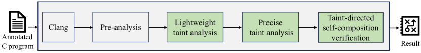
Figure 5. Overview of our approach

3.2. Approach Overview

An overview of our approach is shown in Figure 5. In general, for a given annotated C program, the tool either outputs proved, suggesting that the program is secure, or outputs (potential) side-channel sources and corresponding execution traces for vulnerability localization and repair.

Our approach works as follows. First, the input program is translated into LLVM intermediate representation (IR) with annotations using Clang, the front-end of LLVM. Second, we compute the call graph, interprocedural control-flow graph, points-to information and definition-use chains required by the subsequent steps via a pre-analysis. Third, a lightweight taint analysis (cf. Section 4.1) is performed by leveraging the inter-procedural, finite, distributive, subset (IFDS) framework (RHS95). Often it is able to determine a large number of potential side-channel sources, leaving few potential side-channel sources unresolved. Finally, we resort to a precise taint analysis (cf. Section LABEL:sect:2ndtaint) and a taint-directed self-composition verification (cf. Section LABEL:sec:cpverif) to resolve the left-over potential side-channel sources. The precise taint analysis reduces the flow-, context-, path-, field- and index-sensitive taint analysis problem to checking safety properties of a cross-product of the given program and its Boolean abstraction which tracks the required information flow from the secrets. The taint-directed self-composition consists of two copies of the original program which is a new variant of self-composition. Remarkably, the taint information is utilized in both cross-product constructions to simplify the resulting program and reduce the cost of safety checks. By combining lightweight taint analysis and heavyweight safety verification, the overall approach brings the best of three worlds: efficiency, soundness and theoretical completeness.

Consider the motivating examples. The lightweight taint analysis is able to prove that all the five potential side-channel sources in Example 1 actually do not leak secrets, so the next two steps are not needed. In Example 2, the lightweight taint analysis fails to determine the potential side-channel source $(11,{\tt!j12})$, thus the subsequent analyses have to check $(11,{\tt!j12})$, which can be resolved by the precise taint analysis. (The final step is thus not needed.) We remark that the precise taint analysis may fail to prove some constant-time implementations meaning that it is sound but incomplete. For instance, when the secret $k$ is involved in the computation of a potential timing side-channel source $x$ (e.g., $x=k\oplus p\oplus k$ where $\oplus$ is Exclusive-OR), and the value of $x$ is independent upon the secret $k$, the precise taint analysis will raise a false positive.

4. Methodology

In this section, we present the details of the three key components, i.e., lightweight taint analysis, precise taint analysis and taint-directed self-composition.

4.1. Lightweight Taint Analysis

In this subsection, we present a lightweight taint analysis which is designed to be flow-, field- and context-sensitive, but path-and index-insensitive, for a balance of efficiency and precision. Often it is able to prove that a large number of potential side-channel sources do not leak secrets, leaving few potential side-channel sources unresolved.

Taint source. Fix a safe program ${\tt P}$. The taint source is the set $\mathbb{X}^{in}_{h}$ of its secret input variables, each of which is a taint fact. We remark that although our implementation supports the element-wise annotation of input array variables, this taint analysis is index-insensitive. Thus, if any element of an input array variable is annotated by secret, the array variable is regarded as secret, i.e., all the elements of the array are tainted.

$\inference{T^{\prime}=\big{(}y\in T\ ?\ T\cup\{x\}:T\setminus\{x\}\big{)}}{x:=y[z]\vdash T\hookrightarrow T^{\prime}}[T-{\sc Assign}$_1$]$	$\inference{T^{\prime}=\big{(}{\tt var}(e)\cap T\neq\emptyset\ ?\ T\cup\{x\}:T\setminus\{x\}\big{)}}{x:=e\vdash T\hookrightarrow T^{\prime}}[T-{\sc Assign}$_3$]$
$\inference{T^{\prime}=\big{(}z\in T\ ?\ T\cup\{x\}:T\big{)}}{x[y]:=z\vdash T\hookrightarrow T^{\prime}}[T-{\sc Assign}$_2$]$	$\inference{p\mbox{ is }{\color[rgb]{0,0,1}\tt skip}\mbox{ or }{\color[rgb]{0,0,1}\tt assert}\ e\mbox{ or }{\color[rgb]{0,0,1}\tt assume}\ e}{p\vdash T\hookrightarrow T}[T-{\sc Identity}]$
p2⊢T1↪T′p1;p2⊢T