Push Quantization-Aware Training Toward Full Precision Performances via Consistency Regularization

Abstract

Existing Quantization-Aware Training (QAT) methods intensively depend on the complete labeled dataset or knowledge distillation to guarantee the performances toward Full Precision (FP) accuracies. However, empirical results show that QAT still has inferior results compared to its FP counterpart. One question is how to push QAT toward or even surpass FP performances. In this paper, we address this issue from a new perspective by injecting the vicinal data distribution information to improve the generalization performances of QAT effectively. We present a simple, novel, yet powerful method introducing Consistency Regularization (CR) for QAT. Concretely, CR assumes that augmented samples should be consistent in the latent feature space. Our method generalizes well to different network architectures and various QAT methods. Extensive experiments demonstrate that our approach significantly outperforms the current state-of-the-art QAT methods and even FP counterparts.

1 Introduction

Model compression has emerged as an inevitable imperative to deploy deep models on edge devices. Classical approaches in the model compression community include neural architecture search [1], network pruning [2] and quantization [3; 4]. Among these approaches, due to its generality in engineering, quantization benefits existing artificial intelligence (AI) accelerators, which generally focus on low-precision arithmetic, resulting in lower latency, smaller memory footprint, and less energy consumption. Categorically, quantization can be divided into two classes: Post-Training Quantization (PTQ) [5; 6; 7] and Quantization-Aware Training (QAT) [8; 9]. PTQ finetunes the quantized network using a small calibration set without retraining. Consequently, PTQ offers a fast and straightforward approach. However, at low bits, such as 2/4-bit widths, PTQ faces a massive drop in performance. On the contrary, QAT retrains a neural network to preserve accuracy under a low-bit-width model.

Table 1: Accuracies ($\%$) comparison among FP32, LSQ and our method with 2W4A quantization in terms of accuracy on CIFAR-10. ResNet-18 is used as a baseline model. We report the average of 10 seeds and the STD.

# Test samples	5,000 train samples			50,000 train samples
	FP32	LSQ	CR (Ours)	FP32	LSQ	CR (Ours)
1000	65.24±0.74	67.39±1.55	70.49±0.99	88.89±0.82	87.71±0.84	89.49±1.08
2000	64.90±0.64	65.99±0.83	71.33±0.81	88.58±0.97	87.90±0.50	89.58±0.63
3000	64.62±0.58	66.38±1.21	70.67±0.54	89.10±0.62	87.53±0.40	90.06±0.52
4000	65.86±0.54	66.30±0.60	70.90±0.53	88.72±0.44	87.75±0.39	89.70±0.41
5000	65.17±0.42	65.87±0.33	71.08±0.56	88.75±0.22	87.54±0.38	89.62±0.30
6000	64.58±0.44	65.90±0.39	70.98±0.39	88.65±0.24	87.65±0.28	89.80±0.26
7000	64.82±0.22	65.71±0.17	70.96±0.36	88.66±0.29	88.87±0.36	89.74±0.16
8000	64.51±0.29	65.87±0.22	70.90±0.15	88.62±0.17	87.67±0.22	89.69±0.13
9000	64.62±0.16	65.67±0.38	70.97±0.13	88.75±0.09	87.76±0.11	89.72±0.11

Although QAT makes a significant effort to improve the performance with complete datasets, the accuracy of QAT is still lower than that of its FP counterpart. As shown in Tab. 1, as the size of the testing set increases, the State-Of-The-Art (SOTA) Learned Step Size Quantization (LSQ) [8] has inferior performances compared to the FP counterpart. One of the main reasons leading to this phenomenon is the oscillation of weights around decision boundaries due to the approximate gradient estimation [10; 9]. As shown in Fig. 5, the oscillation prevents the quantized model from learning an effective weight distribution for the quantization task. Nevertheless, QAT leverages complete datasets and has expensive computational overhead. Naturally, one question is how to push QAT toward FP accuracy and even surpass the FP counterpart. Intuitively, a viable solution is to improve the generalization as a more accurate approximation of the actual distribution.

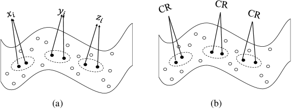
Figure 1: Comparison between cross entropy and CR. (a) cross-entropy (b) CR.

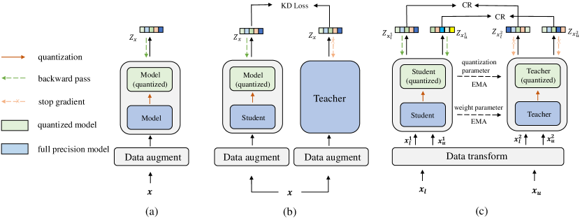
Figure 2: Comparison between vanilla QAT, quantization with KD [11] and our method. (a) the overview of vanilla QAT. (b) the overview of quantization with KD. (c) the overview of our method.

In this paper, we assume that the vicinal data distribution via sample perturbation supplies supervision signals to guarantee the generalization ability of a quantized model, as shown in Fig. 1 (b). This idea intuitively expects a stable quantized network under the perturbation of samples. A naive approach is to increase the types of data arguments during the traditional QAT, shown in Fig. 2(a). However, this simple approach does not exploit more supervision signals than the traditional approaches [8; 12]. Therefore, except for the label information, exploiting the supervision signals from unlabeled vicinal data distribution is natural solution. The unlabeled vicinal data distribution has many potential benefits: reducing the annotations cost, making quantized models stable, and removing the bias of the supervised method [13].

Therefore, except for the label information in Fig. 1 (a), it is natural to exploit the supervision signals from unlabeled vicinal data distribution to increase the generalization ability in Fig. 1 (b). In this paper, we propose Consistency Regularization (CR) to harness generalization ability by the consistency between two augmented samples from an unlabeled datum. As illustrated in Fig. 2 (c), a student network represents any QAT model. In contrast, a teacher network is a temporal ensemble of student networks in the parameter space. Theoretically, CR could be any method to measure the divergence between the student network and the teacher one, enforcing a quantized model to learn the vicinal feature distribution of each sample.

Further, in injecting vicinal data distribution of a sample, rather than adopting the Knowledge Distillation (KD) [14; 15] (which is a common approach in QAT) and a standard data arguments (which is also the most celebrated preprocessing method), we instead propose CR in the hope of mining local consistency to retain the generalization ability. Our contributions are as follows:

• To our best knowledge, we are the first to harness vicinal data distribution from unlabeled samples to improve the generalization ability of quantized models. The supervision signals from the data distribution are considered complementary information for labels.

• We propose a training paradigm for QAT based on CR. The proposed approach, a simple, novel, yet powerful method, is easily adapted to different neural networks. CR pushes the performances of QAT models towards and surpasses that of FP32 counterparts, especially at the low bit widths.

• Extensive experiments on different models prove that our method set up a new SOTA method for QAT, validating the power of unlabeled data in model quantization.

2 Related Work

Quantization-Aware Training. The idea of QAT is to minimize quantization errors by the complete training dataset, enabling the network to consider task-related loss. There are two research directions in QAT: 1) one primarily focuses on addressing quantization-specific issues, such as gradient backpropagation caused by rounding operations [16; 17] and weight oscillations during the training stage [9]; 2) the other integrates quantization with other training paradigms.

For the first category, STE [16] employed the expected probability of stochastic quantization as the derivative value in backpropagation. EWGS [17] adaptively scaled quantized gradients based on quantization error, compensating for the gradient. PSG [18] scaled gradients based on the position of the weight vector, essentially providing gradient compensation. DiffQ [10] found that STE can cause weight oscillations during training and thus employed additive Gaussian noise to simulate quantization noise. It is overcoming Oscillations Quantization [9] addressed oscillation issues by introducing a regularization term that encourages latent weights to be close to the center of the bin. ReBNN [19] introduced weighted reconstruction loss to establish an adaptive training objective. The balance parameter associated with the reconstruction loss controls the weight oscillations.

In addition to addressing quantization-specific issues, some approaches integrate quantization with other training paradigms. SSQL [20] unified self-supervised learning and quantization to learn quantization-friendly visual representations during pre-training. [21] effectively combined quantization and distillation, inducing the training of lightweight networks with solid performance.

However, these methods focus on approximating gradients or utilizing KD to retain performances. To this end, we propose a method to push toward and surpass that of FP32 counterparts with only unlabeled data.

Generalization in quantization. The generalization ability of quantization models is barely discussed. [22] employed Iterative Product Quantization (IPQ) to reduce the interdependence between weights and enhance model generalization. QDrop [7] introduced a noise scheme by randomly dropping activation quantization and achieving a flatness of loss landscape. However, their approach is not readily adopted by QAT. [23] introduced Stochastic Weight Averaging (SWA). Concretely, at the end of each periodic training cycle, the weights are averaged using SWA, which mimics the flatness of a loss landscape. It is seemingly like our method, but it’s different from the problem we’re solving. We leverage the vicinal data distribution to address quantization networks’ generalization issue and oscillation phenomenon.

Unlabeled data for generalization. Unlabeled data are widely applied in Self-Supervised Learning (SfSL) [24; 25] and Semi-Supervised Learning(SiSL) [26; 27]. SfSL aimed to learn the representations from unlabeled data for the downstream tasks. SiSL utilized a substantial amount of unlabeled data and a limited amount of labeled data to generate pseudo-labels for unlabeled data. For example, temporal ensembling [28] employed EMA to generate pseudo-labels. Mean Teacher (MT) [29] minimized the performance gap between teacher and student networks. [30] used data augmentation on unlabeled data and applied consistency training. Our method follows the same idea of SiSL to improve the model’s generalization ability by perturbing the input space.

3 Methodology

This section introduces our approach, CR for quantization. We begin with the basic notation and a brief review of previous works, followed by our algorithm and analysis.

3.1 Notation and Background

Basic Notations. In this paper, notation $\mathbf{X}$ represents a matrix (or tensor), the vector is denoted as $\mathbf{x}$, labeled data is $\mathbf{x}_{l}$, and unlabeled data is $\mathbf{x}_{u}$. $S(\mathbf{x};\mathbf{w}$) represents the model $S\left(\cdot;\cdot\right)$ with the parameter $\mathbf{w}$ and the input $\mathbf{x}$.

For a neural network with activation, we denote the loss function as $L\left(\mathbf{w},\mathbf{x}\right)$, where $\mathbf{w}$ and $\mathbf{x}$ represent the network’s weights and input, respectively. Note that we assume $\mathbf{x}$ is sampled from the training set $\mathcal{D}_{t}$, thus the final loss is defined as $\mathbb{E}_{\mathbf{x}\sim\mathcal{D}_{t}}[L\left(\mathbf{w},\mathbf{x}\right)]$.

Quantization. Quantization parameters steps $s$ and zero points $z$ serve as a bridge between floating-point and fixed-point representations. Given the input tensor $\mathbf{x}$, the quantization operation is as follows:

$$\mathbf{x}_{int} =clip\left(\lfloor{\frac{\mathbf{x}}{s}}\rceil+z,0,2^{q}-1\right)$$ (1)

$$\hat{\mathbf{x}} =\left(\mathbf{x}_{int}-\mathbf{z}\right)s,$$

where $\lfloor{\cdot}\rceil$ represents the rounding-to-nearest operator, $q$ is the predefined quantization bit-width, $\mathbf{s}$ denotes the step size between two subsequent quantization levels. $\mathbf{z}$ stands for the zero-points. The $s$ and $z$ is initialized through forward propagation by a calibration set $\mathcal{D}_{c}$ ($\mathcal{D}_{c}\in\mathcal{D}_{t}$) from the training dataset$\mathcal{D}_{t}$.

$$s=\frac{\mathbf{x}_{max}-\mathbf{x}_{min}}{2^{q}-1}.$$ (2)

Different from LSQ [8], the quantization parameter $\mathbf{s}$ is calibrated by samples. Therefore, the loss function of a quantized model is given as follows:

$$\mathop{\arg\min}_{\hat{\mathbf{w}}}\ \ \mathbb{E}_{\mathbf{x}\sim\mathcal{D}_{t}}[L\left(\hat{\mathbf{w}},\mathbf{x}\right)],$$ (3)

where $\hat{\mathbf{w}}$ is the quantized weight obtained from the latent weight $\mathbf{w}$ after quantization by (1).

3.2 Consistency Regularization

Figure 3: Augmented samples

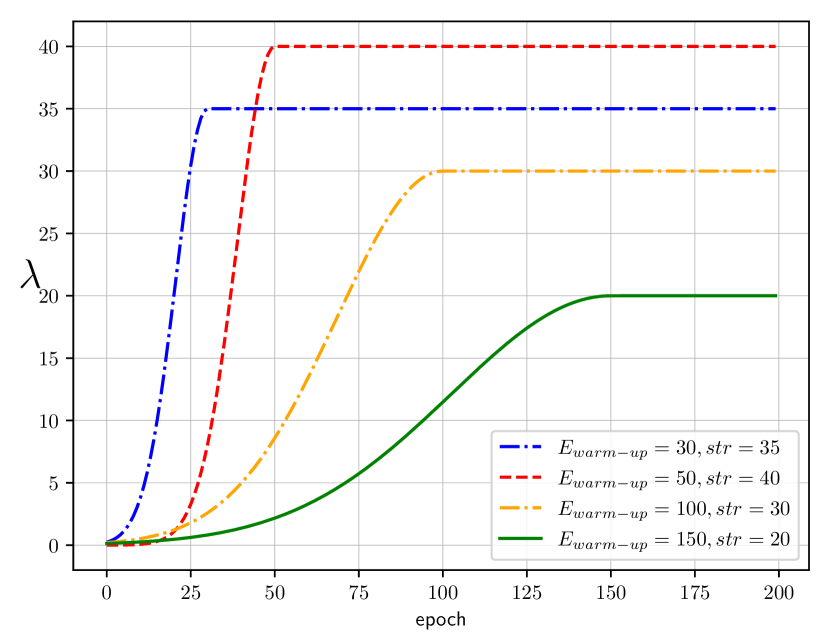
Figure 4: Different settings of $\lambda$

The framework of CR is shown in Fig. 2(c). Both the student model $S\left(\mathbf{x};\mathbf{w}\right)$ and the teacher model $T\left(\mathbf{x};\mathbf{w}\right)$ are the ones that we aim to quantize. They are first initialized with the same calibration dataset.

We obtain an FP teacher model by utilizing EMA to the weights of the FP student. This ensures that the FP teacher model handles the weight oscillations phenomenon [9]; we also apply EMA to the learnable quantization parameters in the teacher model to maintain the stability of quantization parameters. The parameters of the teacher model are updated as follows:

$$T\left(\mathbf{w}_{t}\right)=\alpha T\left(\mathbf{w}_{t-1}\right)+\left(1-\alpha\right)S\left(\mathbf{w}_{t}\right),$$ (4)

where index $t$ is the $t$-th mini-batch iteration, and $\alpha$ ($\alpha>0$) is a smoothing weight. In this paper, we set $\alpha=0.999$. Therefore, (4) results in a more stable teacher model than the student model.

Given a labeled sample $(\mathbf{x}_{l},y)$ and the corresponding label $y$, as well as unlabeled sample $\mathbf{x}_{u}$, each sample $\mathbf{x}$ is augmented into two distinct views. We aim to maintain consistent predictions from the data perturbations for the same sample, thereby enhancing the generalization ability of the quantized model. Concretely, the augmented data in Fig. 2 (c) is represented as follows:

$$\mathbf{x}^{1}_{l},\mathbf{x}^{2}_{l} =DataAug\left(\mathbf{x}_{l};\theta\right)$$ (5)

$$\mathbf{x}^{1}_{u},\mathbf{x}^{2}_{u} =DataAug\left(\mathbf{x}_{u};\theta\right)$$ (6)

where $DataAug(\mathbf{x};\theta)$ is the data augmentation function controlled by the parameter $\theta$, in which $\theta$ determines the types of data augmentation (such as horizontal flip, random translation for image-based classification) and their strength (please refer Sec 4.2 for details). The augmented samples are shown in Fig. 4. The labeled data $\mathbf{x}_{l}$ and the unlabeled data $\mathbf{x}_{u}$ are mixed into a mini-batch according to a particular proportion, such as 1:7.

Given the two transformed samples $\mathbf{x}^{1}_{l}$ and $\mathbf{x}^{1}_{u}$, the student model $S(\mathbf{x};\mathbf{w})$ generates two outputs $\mathbf{z}_{\mathbf{x}_{1}}$and $\mathbf{z}_{\mathbf{u}_{1}}$ as follows:

$$\mathbf{z}_{\mathbf{x}^{1}_{l}}=S(\mathbf{x}^{1}_{l};\mathbf{w}_{S})$$ (7)

$$\mathbf{z}_{\mathbf{x}^{1}_{u}}=S(\mathbf{x}^{1}_{u};\mathbf{w}_{S})$$

similarly, given the two transformed data $\mathbf{x}^{2}_{l}$ and $\mathbf{x}^{2}_{u}$, the teacher model $T(\mathbf{x};\mathbf{w})$ generates two outputs $\mathbf{z}_{\mathbf{x}_{2}}$and $\mathbf{z}_{\mathbf{u}_{2}}$.

$$\mathbf{z}_{\mathbf{x}^{2}_{l}}=T(\mathbf{x}^{2}_{l};\mathbf{w}_{T})$$ (8)

$$\mathbf{z}_{\mathbf{x}^{2}_{u}}=T(\mathbf{x}^{2}_{u};\mathbf{w}_{T})$$

where $\mathbf{w}_{S}$ in (7) and $\mathbf{w}_{T}$ in (8) are the quantized weight matrices of the student model $S(\mathbf{x};\mathbf{w})$ and teacher model $T(\mathbf{x};\mathbf{w})$, respectively.

A quantization model is expected to effectively exploit the vicinal data distribution to reduce the sensitivity to noise and local transformations. Therefore, we impose CR between the outputs $\mathbf{z}_{\mathbf{x}^{1}_{l}}$ ($\mathbf{z}_{\mathbf{x}^{1}_{u}}$) and $\mathbf{z}_{\mathbf{x}^{2}_{l}}$ ($\mathbf{z}_{\mathbf{x}^{2}_{u}}$) from two different views of the same image $\mathbf{x}_{l}$ ($\mathbf{x}_{u}$) as follows:

$$L_{CR}\left(\hat{\mathbf{w}},\mathbf{x}\right)=J\left(\mathbf{z}_{\mathbf{x}^{1}_{u}},\mathbf{z}_{\mathbf{x}^{2}_{u}}\right)+J\left(\mathbf{z}_{\mathbf{x}^{1}_{l}},\mathbf{z}_{\mathbf{x}^{2}_{l}}\right),$$ (9)

where $J(x,y)$ is a consistency loss that reflects the divergence between $x$ and $y$. Both the KL divergence and Mean Squared Error (MSE) could be used to measure the divergence. A vicinal distribution around each sample is built by (9), and further, the global data distribution of the whole dataset is implicitly built.

3.3 Training Processing

In this paper, we focus on the classification task. Therefore, the whole loss consists of two components as follows:

$$L_{total}\left(\hat{\mathbf{w}},\mathbf{x}\right)=CE\left(\mathbf{z}_{\mathbf{x}^{1}_{l}},y\right)+\lambda L_{CR}\left(\hat{\mathbf{w}},\mathbf{x}\right),$$ (10)

where $CE\left(\cdot,\cdot\right)$ denotes the cross-entropy loss for classification tasks, $\mathbf{z}_{\mathbf{x}_{l}}$ presents the output from the student model for the labeled data $(\mathbf{x}_{l},y)$, weight $\lambda$ ($\lambda>0$) balances between the CE loss and CR loss in (9).

The weight $\lambda$ is critical to (10). We have observed that the teacher model’s performance significantly depends on student one. In this paper, $\lambda$ is progressively increased as follows:

$$\lambda=\text{str}\times e^{-5\times\left[1-\left(\frac{\beta}{E_{\text{warm-up}}}\right)^{2}\right]},$$ (11)

where str represents the intensity of CR, $E_{\text{warm-up}}$ represents the predetermined hyperparameter of warm-up epoch, and $\beta$ is:

$$\beta=clip\left(t,0,E_{\text{warm-up}}\right),$$ (12)

where $t$ represents the current epoch.

As illustrated in Fig. 4, (11) assigns a small value to $\lambda$ in the early stages of training, enabling that student model to be well learned from the ground truth. Suppose $\lambda$ makes CR (9) aggressively involved in the early optimization of the loss (10). In that case, the updated teacher model has barely generated a supervised target $\mathbf{z}_{\mathbf{x}}$ for the student model. Gradually, a stable $\lambda$ consistently enforces CR loss to transfer the knowledge from the teacher to the student model. Our overall training algorithm is shown in algorithm 1.

Algorithm 1 QAT with CR

1:  Input: labeled data $\mathbf{X}_{l}$; unlabeled data $\mathbf{X}_{u}$; full precision student model $S\left(\mathbf{x};\mathbf{w}\right)$; full precision teacher model $T\left(\mathbf{x};\mathbf{w}\right)$; iteration $T$.

2:  for $i=1$ to $T$ do

3:     Data Augment for data based on (5);

4:     Feed the data into the quantized student and teacher models based on  (7) and  (8), respectively;

5:     Calculate the CR Loss and the task loss based on (9) and (10);

6:     Update for student model’s weights parameter and quantization parameter $\mathbf{w}$;

7:     Update the parameters $\mathbf{w}$ of the teacher model based on (4);

8:  end for

9:  Output: quantized student model; quantized seacher model.

4 Experiments

Table 2: Comparison among different QAT strategies in terms of accuracy on CIFAR-10 when all the labeled data are used.

Labeled data	Methods	W/A	Res18	Res50	Reg600M	Reg3.2G	MBV1	MBV2
50000	Full Prec.	32/32	88.72	89.95	82.07	87.96	85.52	85.81
50000	PACT (2018)	4/4	88.15	85.27	81.09	85.29	80.77	79.88
	LSQ (2020)	4/4	86.69	90.01	82.12	88.42	82.39	84.45
	LSQ+ (2020)	4/4	88.40	90.30	81.85	87.32	84.32	84.30
	KD(2018)	4/4	88.86	90.34	81.41	87.97	84.77	83.79
	CR (Ours)	4/4	90.48	91.30	84.18	90.02	86.23	85.65
	PACT (2018)	2/4	87.55	85.24	74.49	82.68	69.04	67.18
	LSQ (2020)	2/4	88.36	90.01	81.02	86.96	78.15	78.15
	LSQ+ (2020)	2/4	87.76	89.62	80.22	86.34	81.26	77.00
	KD(2018)	2/4	88.83	90.18	78.53	86.48	78.84	75.56
	CR (Ours)	2/4	89.90	90.13	81.53	88.27	82.86	80.22

In this section, we conduct five sets of experiments to verify the effectiveness of the proposed method. In Sec 4.1, we perform ablation experiments to investigate the impact of CR on both labeled and unlabeled data. In Sec 4.2, we experimentally analyze and discuss the influence of the hyperparameter on the strength of data augment $\theta$. In Sec 4.3, we compare our method with the SOTA QAT methods on CIFAR-10 [31] and ImageNet [32] datasets. In Sec 4.4, we analyze the generalization capability of CR. We visually analyze the weight oscillation phenomenon in Sec 4.5.

Experimental Protocols. Our code is based on PyTorch [33] and relies on the MQBench [34] package. By default, we set the $\beta$ increase linearly from 0 to 4 as the number of epochs increases unless explicitly mentioned otherwise. We use the default method of asymmetric quantization.

In this paper, two datasets, the ImageNet and CIFAR-10, are used. We randomly selected 1,028 images for ImageNet and 100 for CIFAR-10 as the calibration set. We also keep the first and last layers with 8-bit quantization, the same as QDrop [7]. Additionally, we employ per-channel quantization for weight quantization. We use WXAX to represent X-bit weight and activation quantization. We use the labeled examples as the unlabeled samples in CR loss.

Two experimental settings are evaluated as follows:

• (A) We leverage all labeled data and utilize the entire data distribution to enhance the model’s performance and generalization.

• (B) We use 20% labeled data to simulate a scenario with insufficiently labeled data.

Training Details. We use SGD as the optimizer, with a batch size of 256 and a base learning rate of 0.01. The default learning rate (LR) scheduler follows the cosine annealing method. The weight decay is 0.0005, and the SGD momentum is 0.9. We train for 200 epochs on CIFAR-10 and ImageNet unless otherwise specified.

Table 3: Ablation studies of the choice of CR (Accuracy $\%$) on CIFAR-10.

$J\left(\mathbf{Z}_{\mathbf{x}^{1}_{l}},\mathbf{Z}_{\mathbf{x}^{2}_{l}}\right)$	$J\left(\mathbf{Z}_{\mathbf{x}^{1}_{u}},\mathbf{Z}_{\mathbf{x}^{2}_{u}}\right)$	ResNet-18	MobileNetV2
		85.89	75.27
✓		87.19	76.77
	✓	88.10	78.27
✓	✓	88.56	78.47

4.1 Ablation Study

We use 20,000 samples as labeled data and all the remaining samples as unlabeled data to verify the effects of CR on CIFAR-10 in Tab. 3. The pre-trained FP models, ResNet-18 [35] with 88.72$\%$ accuracy and MobileNetV2 [36] with 85.51$\%$, are used as the baselines. As shown in Table 3, CR improves the accuracy of ResNet and MobileNet on CIFAR-10. Both the unlabeled and labeled data would improve the accuracies of the W4A4 quantized model by CR; besides, the more data is used, the more gain the CR supplies.

Tab. 3 also indicates that if we could find enough unlabeled in-distribution samples, CR would significantly improve the accuracy. To valid this observation, following the setting (B), Tab. 5 illustrated that CR significantly outperforms STOA methods, such as LSQ LSQ+. For instance, CR (83.2$\%$) significantly surpasses the PF (77.67$\%$) when the W2A4 setting is used. KD injects the supervision signals via the “soft” labels. Empirical results show that CR consistently outperforms these STOAs using different neural architectures.

Table 4: Ablation studies of different data augmentations on CIFAR-10.

Data Aug.	Val Acc(%)
RHF	89.19
RHF + RT	89.45
RHF + RT + RR	88.22
RHF + RT + RG	89.76
RHF + RT + CJ	89.90

4.2 Parameter Configuration

Data augmentation is crucial to enhance the effect of consistency regularization. We select several commonly used data augmentations, including weak ones, i.e., Random Horizontal Flip (RHF) and Random Translation (RT), and strong ones like Random Rotation (RR), Random Grayscale (RG), and Color Jitter (CJ). We tested ResNet-18 [35] and used all samples from the CIFAR-10 dataset as labeled data. As shown in Table 4, there is a positive correlation between the strength of data augmentation and accuracy on CIFAR-10. This aligns with the experimental observations in SfSL and SiSL: data augmentation should respect the generation of the dataset. The RHF, RT, and CJ data augmentations are used for CIFAR-10 and ImageNet in the following experiments.

4.3 Literature Comparison

Table 5: Comparison among different QAT strategies regarding accuracy on CIFAR-10 when partial data are used.

Labeled data	Methods	W/A	Res18	Res50	Reg600M	Reg3.2G	MBV1	MBV2
10000	Full Prec.	32/32	77.67	75.50	72.39	78.61	76.59	75.21
10000	PACT (2018)	4/4	78.38	75.74	71.20	76.87	64.60	69.34
	LSQ (2020)	4/4	79.34	77.65	71.62	79.50	74.58	74.89
	LSQ+ (2020)	4/4	79.61	78.05	71.85	78.98	74.30	74.68
	KD(2018)	4/4	81.13	80.00	75.22	82.74	78.22	76.34
	CR (Ours)	4/4	83.97	82.56	75.75	84.32	78.72	75.32
	PACT (2018)	2/4	78.99	75.60	68.60	76.23	53.34	59.67
	LSQ (2020)	2/4	79.06	77.56	70.30	77.83	69.00	73.42
	LSQ+ (2020)	2/4	78.40	77.39	69.53	78.14	68.30	70.71
	KD(2018)	2/4	81.23	79.79	74.16	78.14	72.35	71.23
	CR (Ours)	2/4	83.20	82.36	72.73	83.22	73.90	70.04

CIFAR-10. We selected ResNet-18 and -50 [35] with normal convolutions, MobileNetV1 [37] and V2 [36] with depth-wise separable convolutions, and RegNet [38] with group convolutions as our experimental models.

In Tab. 2, we quantized the weights and activations to 2-bit and 4-bit. We compared our approach with the effective baselines, including LSQ [8], PACT [39], and DSQ [40]. Tab. 2 illustrates that when the entire training set of CIFAR-10 is used as the labeled samples, CR significantly surpasses the baselines. In W4A4 quantization, CR using all labeled samples achieved about 1$\sim$3$\%$ accuracy improvements over LSQ. Furthermore, to explore the ability of CR quantization, we conducted W2A4 quantization experiments. In W2A4 quantization, CR consistently achieved a 1$\sim$3$\%$ accuracy improvement over LSQ in Tab. 2. Even with reduced labeled samples in Tab. 5, CR still exhibited excellent performance. For instance, the W4A4 setting in Tab. 5 shows that CR achieved a 4$\%$ accuracy improvement over ResNet and a 2$\%$ accuracy improvement over MobileNet, respectively; besides, when W2A4 setting is adopted in Tab. 5, CR consistently achieved a 2$\%$ accuracy improvement over ResNet and a 4$\%$ accuracy improvement over MobileNet, respectively.

Table 6: Comparison among different QAT strategies with W4A4 regarding accuracy on ImageNet.

Labeled data	Method	Res18	Res50
Entire dataset	Full Prec.	71.00	77.00
	PACT (2018)	69.20	76.50
	DSQ (2019)	69.56	-
	LSQ (2020)	71.10	76.70
	CR (Ours)	70.85	76.93

ImageNet. We also investigated the effectiveness of CR on the ImageNet dataset. We follow the setting (A) in the experimental configuration. The results are presented in Tab. 6.

Tab. 6 compares our approach with previous SOTA methods. For a fair comparison, we compare the results of FP, PACT [39], DSQ [40], and LSQ [8], respectively. Our method outperforms SOTA results reported by LSQ, which learns the step size. For instance, CR improves Res50’s performance from 76.7$\%$ to 76.93$\%$. CR pushes the W4A4 toward the FP result, i.e., 77.0$\%$.

4.4 Generalization of CR

In this section, we first explored the generalization ability of CR by gradually increasing the number of testing samples. As shown in Tab. 1, we gradually increased the number of test samples from 1,000 to 9,000. Tab. 1 shows that CR significantly surpasses improvement LSQ. Mainly, when setting(B) is adopted, the performance of LSQ exhibited a noticeable decline as the number of test samples increased, accompanied by a more significant standard deviation. In contrast, the performance of CR remained stable with more minor variances.

Inspired by the principle of maximum entropy in information theory, a generalizable representation should be the one that admit the maximum entropy among all plausible representations. Accordingly, optimizing towards maximum entropy leads to representations with good generalization capacity. Consequently, we evaluate the distribution of the weights in neural networks. Concretely, we use the per-channel weight quantization, and use histogram normalization on each kernel for each convolutional layer of the ResNet-18. The number of histogram bins is 70.

The comparisons between LSQ and our method are shown in Tab. 7. Tab. 7 illustrates that without the computationally expensive method to estimate the distribution of the weights, our method implicitly obtains a maximum entropy results for QAT.

Table 7: Comparison among FP, LSQ and our method with respect to information entropy. We utilize the ResNet-18 model and calculate the total sum of information entropy on all convolutional kernels within the model.

Method	FP32	LSQ	CR(Teacher)
Entropy	11803.78	12570.15	12599.46

4.5 Weight Oscillation Phenomenon

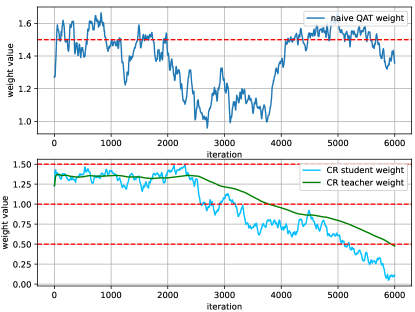
Figure 5: The weight training curve of the first channel in the first convolution of ResNet18 over 2000 iterations on CIFAR-10. The top row plots the weight for the naive QAT, while the bottom plots the weights for the student and teacher models in CR.

In this section, we visualize the weights during the QAT training process. As shown in Fig. 5, the naive QAT training process exhibits severe weight oscillations around the quantization step boundaries, while CR effectively mitigates this issue. In the CR training process, both the EMA-generated teacher model produces the smooth parameter distribution, and the unlabeled data distribution prevents the oscillations at decision boundaries, guiding the student model to learn the effective parameters.

5 Conclusion

In this paper, we propose CR, a simple, novel, yet compelling paradigm for QAT. CR aims to harness vicinal data distribution from unlabeled samples to improve the generalization ability of quantized models. CR pushes the performances of QAT models towards and surpasses that of FP32 counterparts, especially at the low bit widths. Our approach demonstrates promising results across various neural network models. Extensive experiments indicate that our method successfully enhances the generalization ability of the quantized model and outperforms the SOTA approaches in recent QAT research.

References

- [1] Barret Zoph and Quoc V Le. Neural architecture search with reinforcement learning. arXiv preprint arXiv:1611.01578, 2016.
- [2] Song Han, Huizi Mao, and William J Dally. Deep compression: Compressing deep neural networks with pruning, trained quantization and huffman coding. arXiv preprint arXiv:1510.00149, 2015.
- [3] Benoit Jacob, Skirmantas Kligys, Bo Chen, Menglong Zhu, Matthew Tang, Andrew Howard, Hartwig Adam, and Dmitry Kalenichenko. Quantization and training of neural networks for efficient integer-arithmetic-only inference. In Proceedings of the IEEE conference on computer vision and pattern recognition, pages 2704–2713, 2018.
- [4] Sheng Xu, Yanjing Li, Mingbao Lin, Peng Gao, Guodong Guo, Jinhu Lü, and Baochang Zhang. Q-detr: An efficient low-bit quantized detection transformer. In Proceedings of the IEEE/CVF Conference on Computer Vision and Pattern Recognition, pages 3842–3851, 2023.
- [5] Markus Nagel, Rana Ali Amjad, Mart Van Baalen, Christos Louizos, and Tijmen Blankevoort. Up or down? adaptive rounding for post-training quantization. In International Conference on Machine Learning, pages 7197–7206. PMLR, 2020.
- [6] Yuhang Li, Ruihao Gong, Xu Tan, Yang Yang, Peng Hu, Qi Zhang, Fengwei Yu, Wei Wang, and Shi Gu. Brecq: Pushing the limit of post-training quantization by block reconstruction. arXiv preprint arXiv:2102.05426, 2021.
- [7] Xiuying Wei, Ruihao Gong, Yuhang Li, Xianglong Liu, and Fengwei Yu. Qdrop: Randomly dropping quantization for extremely low-bit post-training quantization. arXiv preprint arXiv:2203.05740, 2022.
- [8] Steven K Esser, Jeffrey L McKinstry, Deepika Bablani, Rathinakumar Appuswamy, and Dharmendra S Modha. Learned step size quantization. arXiv preprint arXiv:1902.08153, 2019.
- [9] Markus Nagel, Marios Fournarakis, Yelysei Bondarenko, and Tijmen Blankevoort. Overcoming oscillations in quantization-aware training. In International Conference on Machine Learning, pages 16318–16330. PMLR, 2022.
- [10] Alexandre Défossez, Yossi Adi, and Gabriel Synnaeve. Differentiable model compression via pseudo quantization noise. arXiv preprint arXiv:2104.09987, 2021.
- [11] Antonio Polino, Razvan Pascanu, and Dan Alistarh. Model compression via distillation and quantization. arXiv preprint arXiv:1802.05668, 2018.
- [12] Yash Bhalgat, Jinwon Lee, Markus Nagel, Tijmen Blankevoort, and Nojun Kwak. Lsq+: Improving low-bit quantization through learnable offsets and better initialization. In Proceedings of the IEEE/CVF Conference on Computer Vision and Pattern Recognition Workshops, pages 696–697, 2020.
- [13] Yi Li and Nuno Vasconcelos. Repair: Removing representation bias by dataset resampling. In Proceedings of the IEEE/CVF conference on computer vision and pattern recognition, pages 9572–9581, 2019.
- [14] Yanjing Li, Sheng Xu, Baochang Zhang, Xianbin Cao, Peng Gao, and Guodong Guo. Q-vit: Accurate and fully quantized low-bit vision transformer. Advances in Neural Information Processing Systems, 35:34451–34463, 2022.
- [15] Sheng Xu, Yanjing Li, Bohan Zeng, Teli Ma, Baochang Zhang, Xianbin Cao, Peng Gao, and Jinhu Lü. Ida-det: An information discrepancy-aware distillation for 1-bit detectors. In European Conference on Computer Vision, pages 346–361. Springer, 2022.
- [16] Yoshua Bengio, Nicholas Léonard, and Aaron Courville. Estimating or propagating gradients through stochastic neurons for conditional computation. arXiv preprint arXiv:1308.3432, 2013.
- [17] Junghyup Lee, Dohyung Kim, and Bumsub Ham. Network quantization with element-wise gradient scaling. In Proceedings of the IEEE/CVF conference on computer vision and pattern recognition, pages 6448–6457, 2021.
- [18] Jangho Kim, KiYoon Yoo, and Nojun Kwak. Position-based scaled gradient for model quantization and pruning. Advances in neural information processing systems, 33:20415–20426, 2020.
- [19] Sheng Xu, Yanjing Li, Teli Ma, Mingbao Lin, Hao Dong, Baochang Zhang, Peng Gao, and Jinhu Lu. Resilient binary neural network. In Proceedings of the AAAI Conference on Artificial Intelligence, volume 37, pages 10620–10628, 2023.
- [20] Yun-Hao Cao, Peiqin Sun, Yechang Huang, Jianxin Wu, and Shuchang Zhou. Synergistic self-supervised and quantization learning. In European Conference on Computer Vision, pages 587–604. Springer, 2022.
- [21] Yi Wei, Xinyu Pan, Hongwei Qin, Wanli Ouyang, and Junjie Yan. Quantization mimic: Towards very tiny cnn for object detection. In Proceedings of the European conference on computer vision (ECCV), pages 267–283, 2018.
- [22] Angela Fan, Pierre Stock, Benjamin Graham, Edouard Grave, Rémi Gribonval, Herve Jegou, and Armand Joulin. Training with quantization noise for extreme model compression. arXiv preprint arXiv:2004.07320, 2020.
- [23] Guandao Yang, Tianyi Zhang, Polina Kirichenko, Junwen Bai, Andrew Gordon Wilson, and Chris De Sa. Swalp: Stochastic weight averaging in low precision training. In International Conference on Machine Learning, pages 7015–7024. PMLR, 2019.
- [24] Kaiming He, Haoqi Fan, Yuxin Wu, Saining Xie, and Ross Girshick. Momentum contrast for unsupervised visual representation learning. In Proceedings of the IEEE/CVF conference on computer vision and pattern recognition, pages 9729–9738, 2020.
- [25] Ting Chen, Simon Kornblith, Mohammad Norouzi, and Geoffrey Hinton. A simple framework for contrastive learning of visual representations. In International conference on machine learning, pages 1597–1607. PMLR, 2020.
- [26] Bowen Zhang, Yidong Wang, Wenxin Hou, Hao Wu, Jindong Wang, Manabu Okumura, and Takahiro Shinozaki. Flexmatch: Boosting semi-supervised learning with curriculum pseudo labeling. Advances in Neural Information Processing Systems, 34:18408–18419, 2021.
- [27] Kihyuk Sohn, David Berthelot, Nicholas Carlini, Zizhao Zhang, Han Zhang, Colin A Raffel, Ekin Dogus Cubuk, Alexey Kurakin, and Chun-Liang Li. Fixmatch: Simplifying semi-supervised learning with consistency and confidence. Advances in neural information processing systems, 33:596–608, 2020.
- [28] Samuli Laine and Timo Aila. Temporal ensembling for semi-supervised learning. arXiv preprint arXiv:1610.02242, 2016.
- [29] Antti Tarvainen and Harri Valpola. Mean teachers are better role models: Weight-averaged consistency targets improve semi-supervised deep learning results. Advances in neural information processing systems, 30, 2017.
- [30] Qizhe Xie, Zihang Dai, Eduard Hovy, Thang Luong, and Quoc Le. Unsupervised data augmentation for consistency training. Advances in neural information processing systems, 33:6256–6268, 2020.
- [31] Alex Krizhevsky, Geoffrey Hinton, et al. Learning multiple layers of features from tiny images. 2009.
- [32] Olga Russakovsky, Jia Deng, Hao Su, Jonathan Krause, Sanjeev Satheesh, Sean Ma, Zhiheng Huang, Andrej Karpathy, Aditya Khosla, Michael Bernstein, et al. Imagenet large scale visual recognition challenge. International journal of computer vision, 115:211–252, 2015.
- [33] Adam Paszke, Sam Gross, Francisco Massa, Adam Lerer, James Bradbury, Gregory Chanan, Trevor Killeen, Zeming Lin, Natalia Gimelshein, Luca Antiga, et al. Pytorch: An imperative style, high-performance deep learning library. Advances in neural information processing systems, 32, 2019.
- [34] Yuhang Li, Mingzhu Shen, Jian Ma, Yan Ren, Mingxin Zhao, Qi Zhang, Ruihao Gong, Fengwei Yu, and Junjie Yan. Mqbench: Towards reproducible and deployable model quantization benchmark. arXiv preprint arXiv:2111.03759, 2021.
- [35] Kaiming He, Xiangyu Zhang, Shaoqing Ren, and Jian Sun. Deep residual learning for image recognition. In Proceedings of the IEEE conference on computer vision and pattern recognition, pages 770–778, 2016.
- [36] Mark Sandler, Andrew Howard, Menglong Zhu, Andrey Zhmoginov, and Liang-Chieh Chen. Mobilenetv2: Inverted residuals and linear bottlenecks. In Proceedings of the IEEE conference on computer vision and pattern recognition, pages 4510–4520, 2018.
- [37] Andrew G Howard, Menglong Zhu, Bo Chen, Dmitry Kalenichenko, Weijun Wang, Tobias Weyand, Marco Andreetto, and Hartwig Adam. Mobilenets: Efficient convolutional neural networks for mobile vision applications. arXiv preprint arXiv:1704.04861, 2017.
- [38] Ilija Radosavovic, Raj Prateek Kosaraju, Ross Girshick, Kaiming He, and Piotr Dollár. Designing network design spaces. In Proceedings of the IEEE/CVF conference on computer vision and pattern recognition, pages 10428–10436, 2020.
- [39] Jungwook Choi, Zhuo Wang, Swagath Venkataramani, Pierce I-Jen Chuang, Vijayalakshmi Srinivasan, and Kailash Gopalakrishnan. Pact: Parameterized clipping activation for quantized neural networks. arXiv preprint arXiv:1805.06085, 2018.
- [40] Ruihao Gong, Xianglong Liu, Shenghu Jiang, Tianxiang Li, Peng Hu, Jiazhen Lin, Fengwei Yu, and Junjie Yan. Differentiable soft quantization: Bridging full-precision and low-bit neural networks. In Proceedings of the IEEE/CVF international conference on computer vision, pages 4852–4861, 2019.