An Example Article

Algebraic Riccati Tensor Equations with Applications in Multilinear Control Systems

Abstract

In a recent interesting paper [8], Chen et al. initialized the control-theoretic study of a class of discrete-time multilinear time-invariant (MLTI) control systems, where system states, inputs and outputs are all tensors endowed with the Einstein product. Criteria for fundamental system-theoretic notions such as stability, reachability and observability are established by means of tensor decomposition. The purpose of this paper is to continue this novel research direction. Specifically, we focus on continuous-time MLTI control systems. We define Hamiltonian tensors and symplectic tensors and establish the Schur-Hamiltonian tensor decomposition and symplectic tensor singular value decomposition (SVD). Based on these we propose the algebraic Riccati tensor equation (ARTE) and show that it has a unique positive semidefinite solution if the system is stablizable and detectable. A tensor-based Newton method is proposed to find numerical solutions of the ARTE. The tensor version of the bounded real lemma is also established. A first-order robustness analysis of the ARTE is conducted. Finally, a numerical example is used to demonstrate the proposed theory and algorithms.

15A69, 93B35, 93C05, 93D15

1 Introduction

As natural extension of vectors (1D arrays) and matrices (2D arrays) to higher dimensional arrays, tensors are flexible in representing data and able to characterize high-order interactions. Thus, tensors have found wide applications in a multitude of fields such as signal processing, social and biological networks, scientific computing, and quantum physics [29, 9, 33, 42, 38, 14, 49, 37]. For example, in biological networks, the classic Lotka-Volterra model has recently been extended to including higher-order interactions among species in order to better describe nonlinear interactions, therefore the system evolution is governed by tensors [31]. In [11], stability analysis of the higher-order Lotka-Volterra mode has been conducted.

The Einstein product for tensors is widely used in various fields such as astrophysics [15], elastodynamics [25], data processing [6], and hypergraphs [41]. Due to their important applications in numerical solvers for partial differential equations, continuum physics and engineering problems, tensor equations via the Einstein product have attracted a lot of attention. For example, tensor Krylov subspace methods are designed for solving the Sylvester tensor equation [16, 23, 1, 21].

In [47, 45, 13] the authors studied a class of discrete-time multilinear time-invariant (MLTI) system of the form

(1) $$\mathcal{X}_{t+1}=\mathcal{X}_{t}\times_{1}A_{1}\times_{2}\cdots\times_{N}A_{N},\ \ \mathcal{Y}_{t}=\mathcal{X}_{t}\times_{1}C_{1}\times_{2}\cdots\times_{N}C_{N},$$

where $\mathcal{X}_{t}$ is the state tensor and $\mathcal{Y}_{t}$ is the output tensor at time instant $t$, $A_{n}$ and $C_{n}$ are constant matrices, and “$\times_{j}$” is the mode product commonly used in tensor operations (Definition A.1). These authors numerically demonstrated the superior performance of the MLTI system (1) compared to the classical discrete-time linear time-invariant (LTI) systems in skeleton-based human behavior recognition [13], the modeling of regional climate change [45] and dynamic texture videos [47]. Multipartite quantum states can be nicely represented by tensors [42, Chapter 9]. For example, it is shown in [49] that the steady-state response of a stable quantum linear passive system driven by a multi-channel multi-photon input state can be compactly represented in terms of tensors; essentially speaking, the output tensor is the higher-order SVD (HOSVD) of the input tensor (served as the core tensor) and the impulse response matrix function (or equivalently the transfer matrix function) of the system. If the input tensor passes through a series of quantum systems sequentially, the dynamics are described by the MLTI system (1) with time-varying matrices $A_{n}$.

In recent works [7, 8], Chen et al. generalized the MLTI system (1) using the Einstein product and even-order paired tensors, and proposed the following discrete-time MLTI control systems

(2) $$\mathcal{X}_{t+1}=\mathcal{A}*\mathcal{X}_{t}+\mathcal{B}*\mathcal{U}_{t},\ \ \mathcal{Y}_{t}=\mathcal{C}*\mathcal{X}_{t},$$

in which “$*$” stands for the Einstein product (Definition 2.2), the input $\mathcal{U}_{t}$, output $\mathcal{Y}_{t}$, and state $\mathcal{X}_{t}$ are discrete-time $N$th-order tensorial processes, while $\mathcal{A},\mathcal{B},\mathcal{C}$ are constant $2N$th-order paired tensors. The system (1) can be obtained from the system (2) when $\mathcal{A}=A_{1}\circ A_{2}\circ\cdots\circ A_{N},\mathcal{C}=C_{1}\circ C_{2}\circ\cdots\circ C_{N}$ and $\mathcal{B}=\mathcal{O}$ (the zero tensor). Stability, reachability and observability for discrete-time MLTI systems (2) are established under the framework of tensor algebraic theory, which are generalizations of the control theory.

However, in many scenarios, tensorial time series such as those in computer vision and financial data analysis are tensor-valued processes on continuous time intervals, and the observed multidimensional data are discretizations of the underlying continuous-time tensor-valued process [3]. The tensor-valued differential equations [2, 3] are proposed for modeling the underlying continuous-time tensorial processes in multimodal dynamical systems, which successfully preserve the data spatial and latent continuous sequential information.

Inspired by the above studies, in this paper we study a class of continuous-time MLTI system of the form

(3) $$\dot{\mathcal{X}}(t)=\mathcal{A}*\mathcal{X}(t)+\mathcal{B}*\mathcal{U}(t),\ \ \mathcal{Y}(t)=\mathcal{C}*\mathcal{X}(t)+\mathcal{D}*\mathcal{U}(t),$$

where the state $\mathcal{X}(t)$, input $\mathcal{U}(t)$, and output $\mathcal{Y}(t)$ are continuous-time $N$th-order tensor processes, while $\mathcal{A},\mathcal{B},\mathcal{C},\mathcal{D}$ are constant $2N$th-order paired tensors. Clearly, system (3) contains the system $\dot{\mathcal{X}}_{t}=\mathcal{X}_{t}\times_{1}A_{1}\times_{2}\cdots\times_{N}A_{N},\ \mathcal{Y}_{t}=\mathcal{X}_{t}\times_{1}C_{1}\times_{2}\cdots\times_{N}C_{N}$ as a special case, which is the continuous-time counterpart of system (1). In particular, we study the following algebraic Riccati tensor equation (ARTE)

(4) $$\mathcal{A}^{\mathrm{H}}*\mathcal{E}+\mathcal{E}*\mathcal{A}-\mathcal{E}*\mathcal{G}*\mathcal{E}+\mathcal{K}=\mathcal{O},$$

where $\mathcal{A,G,K}$ and the unknown tensor $\mathcal{E}$ are even-order paired tensors. When the order $N=1$, the ARTE (4) reduces to the well-known algebraic Riccati equation (ARE)

(5) $$A^{\rm H}E+EA-EGE+K=O.$$

The linear-quadratic optimal control problem is closely related to the positive semidefinite solution of the ARE (5) [30, 50]. Analogously, the minimizer of the multilinear quadratic optimal control problem $\min_{\mathcal{U}}\int_{0}^{\infty}\left(\mathcal{X}^{\rm H}(t)*\mathcal{G}*\mathcal{X}(t)+\mathcal{U}^{\rm H}(t)*\mathcal{K}*\mathcal{U}(t)\right)dt$ for the continuous-time MLTI system (3) is $\mathcal{U}(t)=-\mathcal{B}^{\rm H}*\mathcal{E}*\mathcal{X}(t)$, where $\mathcal{E}$ is the positive semidefinite solution of the ARTE (4) with $\mathcal{G}=\mathcal{B}*\mathcal{B}^{\mathrm{H}}$ and $\mathcal{K}=\mathcal{C}^{\mathrm{H}}*\mathcal{C}$.

The contribution of this paper is two-fold. On one hand, we continue to develop even-order paired tensors theory endowed with the Einstein product. Specifically, we define symplectic tensors (Definition 3.2) and Hamiltonian tensors (Definition 3.3), and propose the Schur-Hamiltonian tensor decomposition (Theorem 3.6) and the symplectic tensor SVD (Theorem 3.9). We define the tensor Vec operation (Definition 3.16) and discuss its properties (Propositions 3.17 and 3.19, and Lemma 3.23) with the tensor Kronecker product (Proposition 3.12 and Corollary 3.14). We present and study a Lyapunov tensor equation (Corollary 3.27). Moreover, we discuss fast computational methods of these operations for some structured tensors (Propositions C.1, C.4, C.7, C.8, and C.9). On the other hand, we develop continuous-time MLTI control theory. In particular, we investigate the existence and uniqueness of the positive semidefinite solution to the ARTE (4), see Theorem 4.5, and conduct a first-order robustness analysis (Section 4.3). Moreover, we present a tensor version of the bounded real lemma (Lemmas 4.1 and 4.7).

The paper is organized as follows. In Section 2, we recall related tensor notations and results. In Section 3, we introduce theories of Hamiltonian and symplectic tensors, define the ‘vectorized’ operation for even-order paired tensors, and study the Sylvester tensor equation and Lyapunov tensor equation. In Section 4, the basic control theory for continuous-time MLTI systems is introduced, the unique existence of the positive semidefinite solution of the ARTE (4) is investigated, and its first-order perturbation analysis is conducted. Section 5 derives the Newton method for the ARTE (4); especially for the ARTE (4) with rank-one coefficient tensors, the computational cost can be saved. Moreover, a numerical example is used to demonstrate the proposed theory and algorithms. Concluding remarks are given in Section 6.

2 Preliminaries

Notation. $\mathbb{C}^{I_{1}\times\cdots\times I_{N}}$ denotes the set of all $N$th-order tensors of dimensions $(I_{1},\dots,I_{N})$ over the complex number field $\mathbb{C}$, where $I_{n}$ is the dimension of the $n$th mode of the tensor. We use calligraphic capital letters such as $\mathcal{X}$, capital letters such as $X$, and boldface lowercase letters such as $\mathbf{x}$ to denote tensors, matrices, and vectors, respectively. Given two vectors of indices $\mathbf{i}=\left(i_{1},\dots,i_{N}\right)$ and $\mathbf{j}=(j_{1},\dots,j_{N})$, let $\mathbf{i}\wedge\mathbf{j}=(i_{1},j_{1},\dots,i_{N},j_{N})$ . The colon notation ‘:’ is used to specify indices range (as in MATLAB). For example, $\mathcal{A}_{i_{1}\cdots i_{N}}$ is the entry of the tensor $\mathcal{A}$ specified by the index vector $\mathbf{i}$, while $\mathcal{A}_{:i_{2}\cdots i_{N}}$ is the vector obtained by fixing indices other than the first one. Given two vectors of mode dimensions $\mathbf{I}=(I_{1},\dots,I_{N})$ and $\mathbf{J}=(J_{1},\dots,J_{N})$, their Hadamard product $\mathbf{I}\odot\mathbf{J}=(I_{1}J_{1},\dots,I_{N}J_{N})$, namely the elementwise product of $\mathbf{I}$ and $\mathbf{J}$. Finally, let $\left|\mathbf{I}\right|=I_{1}\cdots I_{N}$. The vector-valued inequality $\mathbf{1}\leq\mathbf{i}\leq\mathbf{I}$ is understood as $1\leq i_{n}\leq I_{n}$ for all $n=1,\dots,N$.

2.1 Even-order paired tensors

Even-order paired tensors were originally proposed by Huang and Qi [24], based on which Chen et al. [7, 8] developed the control theory for the MLTI systems (2) via the Einstein product.

Definition 2.1 (Even-order paired tensors [7, 8, 24]).

Even-order paired tensors are $2$Nth order tensors with elements specified by a pairwise index notation, i.e., $\mathcal{A}_{i_{1}j_{1}\cdots i_{N}j_{N}}$ with paired indices $(i_{n},j_{n})$ for each $n=1,2,\dots,N$. The $(2n-1)$th mode of $\mathcal{A}$ is called the $n$-mode row, while the $2n$th mode of $\mathcal{A}$ is called the $n$-mode column.

Definition 2.2 (Einstein product [5, 8]).

Given two even-order paired tensors $\mathcal{A}\in\mathbb{C}^{I_{1}\times J_{1}\times\cdots\times I_{N}\times J_{N}}$ and $\mathcal{B}\in\mathbb{C}^{J_{1}\times K_{1}\times\cdots\times J_{N}\times K_{N}}$, the Einstein product $\mathcal{A}*\mathcal{B}$ generates a tensor in $\mathbb{C}^{I_{1}\times K_{1}\times\cdots\times I_{N}\times K_{N}}$, whose entries are

$$\left(\mathcal{A}*\mathcal{B}\right)_{i_{1}k_{1}\cdots i_{N}k_{N}}=\sum_{j_{1}=1}^{J_{1}}\cdots\sum_{j_{N}=1}^{J_{N}}\mathcal{A}_{i_{1}j_{1}\cdots i_{N}j_{N}}\mathcal{B}_{j_{1}k_{1}\cdots j_{N}k_{N}}.$$

Remark 2.3.

We regard an $N$th-order tensor $\mathcal{Y}$ as a $2N$th-order paired tensor whose dimensions of all mode columns (Definition 2.1) are 1. Thus, the definition of the Einstein product for even-order paired tensors can be adopted. For example, if $\mathcal{Y}\in\mathbb{C}^{J_{1}\times\cdots\times J_{N}}$, the Einstein product $\mathcal{A}*\mathcal{Y}\in\mathbb{C}^{I_{1}\times\cdots\times I_{N}}$ is $\left(\mathcal{A}*\mathcal{Y}\right)_{i_{1}\cdots i_{N}}=\sum_{j_{1}=1}^{J_{1}}\cdots\sum_{j_{N}=1}^{J_{N}}\mathcal{A}_{i_{1}j_{1}\cdots i_{N}j_{N}}\mathcal{Y}_{j_{1}\cdots j_{N}}$. If $\mathcal{Y}\in\mathbb{C}^{I_{1}\times\cdots\times I_{N}}$, the Einstein product $\mathcal{Y}^{\rm H}*\mathcal{A}\in\mathbb{C}^{J_{1}\times\cdots\times J_{N}}$ is $\left(\mathcal{Y}^{\rm H}*\mathcal{A}\right)_{j_{1}\cdots j_{N}}=\sum_{i_{1}=1}^{I_{1}}\cdots\sum_{i_{N}=1}^{I_{N}}\overline{\mathcal{Y}_{i_{1}\cdots i_{N}}}\mathcal{A}_{i_{1}j_{1}\cdots i_{N}j_{N}}$, where $\mathcal{Y}^{\rm H}$ denotes the complex conjugate transpose of $\mathcal{Y}$ with entries $(\mathcal{Y}^{\rm H})_{i_{1}\cdots i_{N}}=\overline{\mathcal{Y}_{i_{1}\cdots i_{N}}}$, and we regard $\mathcal{Y}^{\rm H}$ as a $2N$th-order paired tensor while all its dimensions of mode rows are 1.

Tensor unfolding, the process of rearranging the elements of a tensor into a matrix or vector, is a frequently used operation in tensor analysis and numerical computations [5, 29]. Given a sequence of tensor dimensions $\mathbf{I}=\left(I_{1},\dots,I_{N}\right)$ and a corresponding vector of indices $\mathbf{i}=\left(i_{1},\dots,i_{N}\right)$, define

(6) $$\mathrm{ivec}(\mathbf{i},\mathbf{I}):=i_{1}+\sum_{k=2}^{N}(i_{k}-1)\prod_{j=1}^{k-1}I_{j}.$$

Definition 2.4 (Tensor unfolding [5, 8]).

The unfolding process of an even-order paired tensor $\mathcal{A}\in\mathbb{C}^{I_{1}\times J_{1}\times\cdots\times I_{N}\times J_{N}}$ is the isomorphic map $\phi:\mathbb{C}^{I_{1}\times J_{1}\times\cdots\times I_{N}\times J_{N}}\to\mathbb{C}^{|\mathbf{I}|\times|\mathbf{J}|}$ with $\phi(\mathcal{A})=A$ defined componentwise as $\mathcal{A}_{i_{1}j_{1}\cdots i_{N}j_{N}}\overset{\phi}{\rightarrow}A_{\mathrm{ivec}(\mathbf{i},\mathbf{I})\mathrm{ivec}(\mathbf{j},\mathbf{J})}$.

Based on tensor unfolding, some notations for even-order paired tensors analogous to matrices are introduced in [8], which are listed below.

• An even-order paired tensor $\mathcal{D}\in\mathbb{C}^{I_{1}\times I_{1}\times\cdots\times I_{N}\times I_{N}}$ is diagonal if all its entries are $0$ except for $\mathcal{D}_{i_{1}i_{1}\cdots i_{N}i_{N}}$. Moreover, if all the diagonal entries $\mathcal{D}_{i_{1}i_{1}\cdots i_{N}i_{N}}=1$, then $\mathcal{D}$ is the identity tensor denoted by $\mathcal{I}_{\mathbf{I}}$, simply written as $\mathcal{I}$ when its dimensions are clear.

• Given $\mathcal{A}\in\mathbb{C}^{I_{1}\times I_{1}\times\cdots\times I_{N}\times I_{N}}$, if there exists a tensor $\mathcal{B}$ of the same size such that $\mathcal{A}*\mathcal{B}=\mathcal{B}*\mathcal{A}=\mathcal{I}$, then $\mathcal{B}$ is called the inverse of $\mathcal{A}$ denoted by $\mathcal{A}^{-1}$.

• For an even-order paired tensor $\mathcal{A}\in\mathbb{C}^{I_{1}\times J_{1}\times\cdots\times I_{N}\times J_{N}}$, the tensor $\mathcal{B}\in\mathbb{C}^{J_{1}\times I_{1}\times\cdots J_{N}\times I_{N}}$ is called the transpose of $\mathcal{A}$ denoted by $\mathcal{A}^{\top}$, if $\mathcal{B}_{j_{1}i_{1}\cdots j_{N}i_{N}}=\mathcal{A}_{i_{1}j_{1}\cdots i_{N}j_{N}}$, and is called the complex conjugate transpose of $\mathcal{A}$ denoted by $\mathcal{A}^{\mathrm{H}}$, if $\mathcal{B}_{j_{1}i_{1}\cdots j_{N}i_{N}}=\overline{\mathcal{A}_{i_{1}j_{1}\cdots i_{N}j_{N}}}$. $\mathcal{A}$ is said to be Hermitian if $\mathcal{A}=\mathcal{A}^{\mathrm{H}}$.

• The unfolding rank of an even-order paired tensor $\mathcal{A}\in\mathbb{C}^{I_{1}\times J_{1}\times\cdots\times I_{N}\times J_{N}}$ is defined as $\mathrm{rank}_{U}(\mathcal{A}):=\mathrm{rank}(\phi(\mathcal{A}))$, and the unfolding determinant of $\mathcal{A}$ is defined as $\mathrm{det}_{U}(\mathcal{A}):=\mathrm{det}(\phi(\mathcal{A}))$.

• An even-order paired Hermitian tensor $\mathcal{A}\in\mathbb{C}^{I_{1}\times I_{1}\times\cdots\times I_{N}\times I_{N}}$ is positive semidefinite if $\mathcal{Y}^{\mathrm{H}}*\mathcal{A}*\mathcal{Y}=\sum_{\mathbf{1}\leq\mathbf{i}\leq\mathbf{I}}\sum_{\mathbf{1}\leq\mathbf{j}\leq\mathbf{I}}\overline{\mathcal{Y}_{i_{1}\cdots i_{N}}}\mathcal{A}_{i_{1}j_{1}\cdots i_{N}j_{N}}\mathcal{Y}_{j_{1}\cdots j_{N}}\geq 0$ for any nonzero $N$th-order tensor $\mathcal{Y}\in\mathbb{C}^{I_{1}\times\cdots\times I_{N}}$, and positive definite if the inequality is strict.

Finally, we say that an even-order paired tensor $\mathcal{T}\in\mathbb{C}^{I_{1}\times I_{1}\times\cdots\times I_{N}\times I_{N}}$ is upper triangular if $\mathcal{T}_{i_{1}j_{1}\cdots i_{N}j_{N}}=0$ for all $\mathrm{ivec}(\mathbf{i},\mathbf{I})>\mathrm{ivec}(\mathbf{j},\mathbf{I})$, and an even-order paired tensor $\mathcal{U}\in\mathbb{C}^{I_{1}\times I_{1}\times\cdots\times I_{N}\times I_{N}}$ is unitary if $\mathcal{U}^{\mathrm{H}}*\mathcal{U}=\mathcal{U}*\mathcal{U}^{\mathrm{H}}=\mathcal{I}$.

2.2 Tensor concatenation and blocks

Like block matrices, block tensors are tensors whose entries are themselves tensors. Here we adopt a compact concatenation approach [7, 8] to construct block tensors.

Definition 2.5 ($n$-mode block tensor [8]).

Let $\mathcal{A},\mathcal{B}\in\mathbb{C}^{I_{1}\times J_{1}\times\cdots\times I_{N}\times J_{N}}$. For each $n=1,\dots,N$, the $n$-mode row block tensor concatenated by $\mathcal{A}$ and $\mathcal{B}$, denoted by $\left[\begin{smallmatrix}\mathcal{A}&\mathcal{B}\end{smallmatrix}\right]_{n}\in\mathbb{C}^{I_{1}\times J_{1}\times\cdots\times I_{n}\times 2J_{n}\times\cdots\times I_{N}\times J_{N}}$, is defined elementwise as

$$(\begin{bmatrix}\mathcal{A}&\mathcal{B}\end{bmatrix}_{n})_{i_{1}j_{1}\cdots i_{N}j_{N}}=\left\{\begin{aligned} &\mathcal{A}_{i_{1}j_{1}\cdots i_{n}j_{n}\cdots i_{N}j_{N}},\ \quad\quad i_{k}=1,\dots,I_{k},j_{k}=1,\dots,J_{k},\forall k,\\ &\mathcal{B}_{i_{1}j_{1}\cdots i_{n}(j_{n}-J_{n})\cdots i_{N}j_{N}},\ i_{k}=1,\dots,I_{k},\forall k,j_{k}=1,\dots,J_{k}\\ &\quad\quad\quad\ \ \quad\quad\quad\quad\quad\quad\mathrm{for}\ k\neq n\ \mathrm{and}\ j_{n}=J_{n}+1,\dots,2J_{n}.\end{aligned}\right.$$

The $n$-mode column block tensor is $\left[\begin{smallmatrix}\mathcal{A}\\ \mathcal{B}\end{smallmatrix}\right]_{n}:=\left[\begin{smallmatrix}\mathcal{A}^{\top}&\mathcal{B}^{\top}\end{smallmatrix}\right]_{n}^{\top}$.

We also denote by $\left[\begin{smallmatrix}\mathcal{A}&\mathcal{B}\\ \mathcal{C}&\mathcal{D}\end{smallmatrix}\right]_{n}=\left[\begin{smallmatrix}\left[\begin{smallmatrix}\mathcal{A}&\mathcal{B}\end{smallmatrix}\right]_{n}\\ \left[\begin{smallmatrix}\mathcal{C}&\mathcal{D}\end{smallmatrix}\right]_{n}\end{smallmatrix}\right]_{n}$ the $n$-mode block tensor concatenated by the $n$-mode row block tensors $\left[\begin{smallmatrix}\mathcal{A}&\mathcal{B}\end{smallmatrix}\right]_{n}$ and $\left[\begin{smallmatrix}\mathcal{C}&\mathcal{D}\end{smallmatrix}\right]_{n}$.

Remark 2.6.

Given two $N$th-order tensors $\mathcal{X}\in\mathbb{C}^{J_{1}\times\cdots\times J_{N}}$, $\mathcal{Y}\in\mathbb{C}^{J_{1}\times\cdots\times J_{N}}$, the $n$-mode column block tensor $\left[\begin{smallmatrix}\mathcal{X}\\ \mathcal{Y}\end{smallmatrix}\right]_{n}\in\mathbb{C}^{J_{1}\times\cdots\times J_{n-1}\times 2J_{n}\times J_{n+1}\times\cdots\times J_{N}}$ can also be defined as in Definition 2.5, by regarding $\mathcal{X},\mathcal{Y}$ as even-order paired tensors (Remark 2.3).

Under the Einstein product, block tensors enjoy properties similar to their matrix counterparts.

Proposition 2.7 ([8]).

Let $\mathcal{A},\mathcal{B}\in\mathbb{C}^{I_{1}\times J_{1}\times\cdots\times I_{N}\times J_{N}}$, $\mathcal{C},\mathcal{D}\in\mathbb{C}^{J_{1}\times I_{1}\times\cdots\times J_{N}\times I_{N}}$. The following properties of block tensors hold for all $n=1,\dots,N$:

1. $\begin{bmatrix}\mathcal{P}*\mathcal{A}&\mathcal{P}*\mathcal{B}\end{bmatrix}_{n}=\mathcal{P}*\begin{bmatrix}\mathcal{A}&\mathcal{B}\end{bmatrix}_{n},\quad for\ \mathcal{P}\in\mathbb{C}^{L_{1}\times I_{1}\times\cdots\times L_{N}\times I_{N}}$.

2. $\begin{bmatrix}\mathcal{C}*\mathcal{Q}\\ \mathcal{D}*\mathcal{Q}\end{bmatrix}_{n}=\begin{bmatrix}\mathcal{C}\\ \mathcal{D}\end{bmatrix}_{n}*\mathcal{Q},\quad for\ \mathcal{Q}\in\mathbb{C}^{I_{1}\times L_{1}\times\cdots\times I_{N}\times L_{N}}$.

3. $\begin{bmatrix}\mathcal{A}&\mathcal{B}\end{bmatrix}_{n}*\begin{bmatrix}\mathcal{C}\\ \mathcal{D}\end{bmatrix}_{n}=\mathcal{A}*\mathcal{C}+\mathcal{B}*\mathcal{D}.$

Given even-order paired tensors $\mathcal{X}_{k}\in\mathbb{C}^{I_{1}\times J_{1}\times\cdots\times I_{N}\times J_{N}}$ $(k=1,\ldots,K_{n})$, one can apply Definition 2.5 successively to create a bigger even-order $n$-mode row block tensor $\begin{bmatrix}\mathcal{X}_{1}&\cdots&\mathcal{X}_{K_{n}}\end{bmatrix}_{n}\in\mathbb{C}^{I_{1}\times J_{1}\times\cdots\times I_{n}\times J_{n}K_{n}\times\cdots\times I_{N}\times J_{N}}$. Based on these constructions, we give the definitions of mode block tensors and tensor blockings, which will be used in Section 3.

Definition 2.8 (Mode block tensor [7, 8]).

Given $|\mathbf{K}|=K_{1}K_{2}\cdots K_{N}$ even-order paired tensors $\mathcal{X}_{m}\in\mathbb{C}^{I_{1}\times J_{1}\times\cdots\times I_{N}\times J_{N}}$ $(m=1,\dots,|\mathbf{K}|)$, the mode row block tensor $\mathcal{X}$ of size $I_{1}\times J_{1}K_{1}\times\cdots\times I_{N}\times J_{N}K_{N}$ can be constructed by tensor concatenations of Definition 2.5 sequentially:

1. Divide the $|\mathbf{K}|$ tensors $\{\mathcal{X}_{1},\mathcal{X}_{2},\dots,\mathcal{X}_{|\mathbf{K}|}\}$ sequentially into $K_{2}\cdots K_{N}$ groups $\{\mathcal{X}_{1},\dots,\mathcal{X}_{K_{1}}\}$, $\{\mathcal{X}_{K_{1}+1},\dots,\mathcal{X}_{2K_{1}}\}$, $\dots$, where each group has $K_{1}$ tensors in order. Then perform the tensor concatenations over these $K_{2}K_{3}\cdots K_{N}$ groups to obtain $K_{2}K_{3}\cdots K_{N}$ 1-mode row block tensors denoted by $\mathcal{X}^{(1)}_{1}=\begin{bmatrix}\mathcal{X}_{1}&\cdots&\mathcal{X}_{K_{1}}\end{bmatrix}_{1},\dots,\mathcal{X}^{(1)}_{K_{2}K_{3}\cdots K_{N}}=\begin{bmatrix}\mathcal{X}_{|\mathbf{K}|-K_{1}+1}&\cdots&\mathcal{X}_{|\mathbf{K}|}\end{bmatrix}_{1}$, respectively, which are $2N$th-order paired tensors in $\mathbb{C}^{I_{1}\times J_{1}K_{1}\times I_{2}\times J_{2}\times\cdots\times I_{N}\times J_{N}}$.

2. Divide the tensors $\{\mathcal{X}_{1}^{(1)},\mathcal{X}_{2}^{(1)},\dots,\mathcal{X}_{K_{2}\cdots K_{N}}^{(1)}\}$ obtained above sequentially into $K_{3}K_{4}\cdots K_{N}$ groups $\{\mathcal{X}_{1}^{(1)},\dots,\mathcal{X}_{K_{2}}^{(1)}\}$, $\{\mathcal{X}_{K_{2}+1}^{(1)},\dots,\mathcal{X}_{2K_{2}}^{(1)}\}$, $\dots$, where each group has $K_{2}$ tensors in order. Then perform the tensor concatenations over these $K_{3}K_{4}\cdots K_{N}$ groups of tensors to obtain $K_{3}K_{4}\cdots K_{N}$ $2$-mode row block tensors denoted by $\mathcal{X}_{1}^{(2)},\dots,\mathcal{X}_{K_{3}K_{4}\cdots K_{N}}^{(2)}\in\mathbb{C}^{I_{1}\times J_{1}K_{1}\times I_{2}\times J_{2}K_{2}\times\cdots\times I_{N}\times J_{N}}$, respectively.

3. Keep repeating the above processes until the last $N$-mode row block tensor is obtained, which is the mode row block tensor $\mathcal{X}\in\mathbb{C}^{I_{1}\times J_{1}K_{1}\times\cdots\times I_{N}\times J_{N}K_{N}}$, denoted by $\mathcal{X}=\begin{vmatrix}\mathcal{X}_{1}&\mathcal{X}_{2}&\cdots&\mathcal{X}_{|\mathbf{K}|}\end{vmatrix}$.

Here the symbol $|\cdots|$ is used to distinguish from the $n$-mode block tensors. The mode column block tensor can be defined in a similar way and is denoted by

$$\begin{vmatrix}\mathcal{X}_{1}^{\top}&\mathcal{X}_{2}^{\top}&\cdots&\mathcal{X}_{|\mathbf{K}|}^{\top}\end{vmatrix}^{\top}\in\mathbb{C}^{I_{1}K_{1}\times J_{1}\times\cdots\times I_{N}K_{N}\times J_{N}}.$$

Definition 2.9 (Tensor blockings [43]).

For a tensor $\mathcal{A}\in\mathbb{C}^{L_{1}\times\cdots\times L_{N}}$, we say that $\{\mathbf{m}^{(1)},\cdots,\mathbf{m}^{(N)}\}$ specifies a blocking for $\mathcal{A}$, if for all $n=1,\dots,N$, $\mathbf{m}^{(n)}=(m_{1}^{(n)},\dots,m_{I_{n}}^{(n)})$ is an $I_{n}$-dimensional vector of positive integers that sum to $L_{n}$, which divides the $n$th mode of $\mathcal{A}$ into $I_{n}$ parts. The blocking identifies $\mathcal{A}$ as an $I_{1}\times\cdots\times I_{N}$ block tensor, whose $\mathbf{i}=(i_{1},\cdots,i_{N})$-th block is a subtensor of size $m_{i_{1}}^{(1)}\times\cdots\times m_{i_{N}}^{(N)}$, denoted by $\mathcal{A}_{[\mathbf{i}]}:=\mathcal{A}(l_{i_{1}-1}^{(1)}+1:l_{i_{1}}^{(1)},\dots,l_{i_{N}-1}^{(N)}+1:l_{i_{N}}^{(N)})$, where $l^{(n)}_{i_{n}}$ denotes the sum of the first $i_{n}$ terms of the vector $\mathbf{m}^{(n)}$, that is, $l^{(n)}_{i_{n}}={\textstyle\sum_{j=1}^{i_{n}}}m_{j}^{(n)}$ for all $i_{n}=1,\dots,I_{n}$ and $n=1,\dots,N$.

Remark 2.10.

For example, the mode column block tensor $\left[\begin{smallmatrix}\mathcal{X}_{1}^{\top}&\cdots&\mathcal{X}_{|\mathbf{K}|}^{\top}\end{smallmatrix}\right]^{\top}$ in Definition 2.8 has a blocking $\{\mathbf{m}^{(1)},\dots,\mathbf{m}^{(2N)}\}$ with $\mathbf{m}^{(2n-1)}=(\underbrace{I_{n},\dots,I_{n}}_{K_{n}\ \mathrm{terms}})$ and $\mathbf{m}^{(2n)}=J_{n}$ for $n=1,\dots,N$.

2.3 Tensor U-eigenvalues and norms

The tensor eigenvalue problem via the Einstein product often arises from elastic mechanics [36, 25], and is further studied in [5, 10, 48], among others. Chen et al. [7, 8] generalized the matrix-based Rayleigh quotient iteration method for computing tensor U-eigenvalues.

Definition 2.11 (Tensor U-eigenvalue [8]).

Given $\mathcal{A}\in\mathbb{C}^{I_{1}\times I_{1}\times\cdots\times I_{N}\times I_{N}}$, if an $N$th-order nonzero tensor $\mathcal{X}\in\mathbb{C}^{I_{1}\times\cdots\times I_{N}}$ and $\lambda\in\mathbb{C}$ satisfy $\mathcal{A}*\mathcal{X}=\lambda\mathcal{X}$, then $\lambda$ and $\mathcal{X}$ are called the U-eigenvalue and U-eigentensor of $\mathcal{A}$, respectively. The tensor $\mathcal{A}$ is said to be stable if all its U-eigenvalues are on the open left half plane.

The tensor Schur decomposition for even-order paired tensors follows directly from [32, Theorem 4.9]. Thus its proof is omitted.

Lemma 2.12 (Tensor Schur decomposition).

Given $\mathcal{A}\in\mathbb{C}^{I_{1}\times I_{1}\times\cdots\times I_{N}\times I_{N}}$, there exist a unitary tensor $\mathcal{U}$ and an upper triangular tensor $\mathcal{T}$ of the same size such that $\mathcal{A}=\mathcal{U}*\mathcal{T}*\mathcal{U}^{\mathrm{H}}$. Moreover, the diagonal entries $\mathcal{T}_{i_{1}i_{1}\ldots i_{N}i_{N}}$ of $\mathcal{T}$ are the U-eigenvalues of $\mathcal{A}$.

The tensor SVD for even-order tensors has been proposed in [5], which for even-order paired tensors is given below.

Lemma 2.13 (Tensor SVD).

The tensor $\mathrm{SVD}$ of an even-order paired tensor $\mathcal{A}\in\mathbb{C}^{I_{1}\times J_{1}\times\cdots\times I_{N}\times J_{N}}$ is $\mathcal{A}=\mathcal{U}*\mathcal{D}*\mathcal{V}^{\rm H}$, where $\mathcal{U}\in\mathbb{C}^{I_{1}\times I_{1}\times\cdots\times I_{N}\times I_{N}}$ and $\mathcal{V}\in\mathbb{C}^{J_{1}\times J_{1}\times\cdots\times J_{N}\times J_{N}}$ are unitary tensors, and $\mathcal{D}\in\mathbb{C}^{I_{1}\times J_{1}\times\cdots\times I_{N}\times J_{N}}$ is a tensor with $\mathcal{D}_{i_{1}j_{1}\cdots i_{1}j_{1}}=0$ for all $\mathbf{i}\neq\mathbf{j}$, whose diagonal entries $\mathcal{D}_{i_{1}i_{1}\cdots i_{N}i_{N}}$ are called the singular values of $\mathcal{A}$.

The outer product of two tensors $\mathcal{X}\in\mathbb{C}^{I_{1}\times\cdots\times I_{N}}$ and $\mathcal{Y}\in\mathbb{C}^{J_{1}\times\cdots\times J_{M}}$ is an $(N+M)$th-order tensor $\left(\mathcal{X}\circ\mathcal{Y}\right)_{i_{1}\cdots i_{N}j_{1}\cdots j_{M}}=\mathcal{X}_{i_{1}\cdots i_{N}}\mathcal{Y}_{j_{1}\cdots j_{M}}$. The inner product of two tensors $\mathcal{X},\mathcal{Y}\in\mathbb{C}^{J_{1}\times\cdots\times J_{N}}$ is $\left\langle\mathcal{X},\mathcal{Y}\right\rangle=\sum_{\mathbf{1}\leq\mathbf{j}\leq\mathbf{J}}\overline{\mathcal{X}_{j_{1}\cdots j_{N}}}\mathcal{Y}_{j_{1}\cdots j_{N}}$, which gives the Frobenius norm $\left\|\mathcal{X}\right\|_{F}:=\sqrt{\left\langle\mathcal{X},\mathcal{X}\right\rangle}=\sqrt{\sum_{\mathbf{1}\leq\mathbf{j}\leq{\mathbf{J}}}\left|\mathcal{X}_{j_{1}\cdots j_{N}}\right|^{2}}$.

Definition 2.14 (Spectral norm [34]).

The spectral norm of $\mathcal{A}$ is defined by $\left\|\mathcal{A}\right\|_{2}:=\sqrt{\lambda_{\rm{max}}(\mathcal{A}^{\mathrm{H}}*\mathcal{A})}$, where $\lambda_{\rm{max}}(\cdot)$ denotes the largest U-eigenvalue.

Remark 2.15 ([48]).

The spectral norm of a tensor $\mathcal{A}$ can be equivalently defined as $\|\mathcal{A}\|_{2}=\sigma_{\rm max}(\mathcal{A})$, namely the largest singular value of $\mathcal{A}$, and it is compatible with the Frobenius norm, that is, $\left\|\mathcal{A}*\mathcal{X}\right\|_{F}\leq\left\|\mathcal{A}\right\|_{2}\left\|\mathcal{X}\right\|_{F}$ for all $\mathcal{X}\in\mathbb{C}^{J_{1}\times\cdots\times J_{N}}$.

3 Hamiltonian tensors and tensor Kronecker product

3.1 Hamiltonian tensors

Ragnarsson and Van Loan [43] studied the unfolding patterns of block tensors: the subblocks of a tensor can be mapped to contiguous blocks in the unfolding matrix through a series of row and column permutations. Specifically, let $s=qr$. $\Pi_{q,r}\in\mathbb{R}^{s\times s}$ is a perfect shuffle permutation defined by

$$\Pi_{q,r}z=\begin{bmatrix}z(1:r:s)\\ z(2:r:s)\\ \vdots\\ z(r:r:s)\end{bmatrix},\ \ \forall z\in\mathbb{C}^{s}.$$

The following lemma is an immediate consequence of [43, Theorem 3.3].

Lemma 3.1.

Given even-order paired tensors $\mathcal{A},\mathcal{B},\mathcal{C},\mathcal{D}\in\mathbb{C}^{I_{1}\times I_{1}\times\cdots\times I_{N}\times I_{N}}$, there exists a permutation matrix $P=Q_{N}\cdots Q_{2}Q_{1}$ such that

$$\phi\left(\begin{bmatrix}\mathcal{A}&\mathcal{B}\\ \mathcal{C}&\mathcal{D}\end{bmatrix}_{n}\right)=P\begin{bmatrix}\phi(\mathcal{A})&\phi(\mathcal{B})\\ \phi(\mathcal{C})&\phi(\mathcal{D})\end{bmatrix}P^{\top},$$

where $Q_{k}=I_{2I_{1}\cdots I_{N}}$ for $k\leq n$, and $Q_{k}=I_{I_{k+1}\cdots I_{N}}\otimes\Pi_{I_{k},2}\otimes I_{I_{1}\cdots I_{k-1}}$ for $k\geq n+1$.

The results to be derived in the sequel can be done for all $n$-mode block tensors for $n=1,\dots,N$. For ease of representation, we present them for the $1$-mode block tensor case and also omit the subscript, i.e., let $\left[\begin{smallmatrix}\mathcal{A}&\mathcal{B}\\ \mathcal{C}&\mathcal{D}\end{smallmatrix}\right]=\left[\begin{smallmatrix}\mathcal{A}&\mathcal{B}\\ \mathcal{C}&\mathcal{D}\end{smallmatrix}\right]_{1}\in\mathbb{C}^{2I_{1}\times 2I_{1}\times I_{2}\times I_{2}\times\cdots\times I_{N}\times I_{N}}$, for $\mathcal{A},\mathcal{B},\mathcal{C},\mathcal{D}\in\mathbb{C}^{I_{1}\times I_{1}\times\cdots\times I_{N}\times I_{N}}$ and $\left[\begin{smallmatrix}\mathcal{X}\\ \mathcal{Y}\end{smallmatrix}\right]=\left[\begin{smallmatrix}\mathcal{X}\\ \mathcal{Y}\end{smallmatrix}\right]_{1}$ for $N$th-order tensors $\mathcal{X},\mathcal{Y}\in\mathbb{C}^{I_{1}\times\cdots\times I_{N}}$. We introduce the block-structured tensor $\mathcal{J}=\left[\begin{smallmatrix}\mathcal{O}&\mathcal{I}\\ -\mathcal{I}&\mathcal{O}\end{smallmatrix}\right]$, where $\mathcal{I},\mathcal{O}$ are the identity tensor and zero tensor respectively. It reduces to the well-known $2\times 2$ block matrix $J=\left[\begin{smallmatrix}O&I\\ -I&O\end{smallmatrix}\right]$ if $N=1$.

Definition 3.2 (Symplectic tensor).

We call $\mathcal{S}\in\mathbb{C}^{2I_{1}\times 2I_{1}\times I_{2}\times I_{2}\times\cdots\times I_{N}\times I_{N}}$ a symplectic tensor if $\mathcal{S}^{\mathrm{H}}*\mathcal{J}*\mathcal{S}=\mathcal{J}$.

Definition 3.3 (Hamiltonian tensor).

We call $\mathcal{M}\in\mathbb{C}^{2I_{1}\times 2I_{1}\times I_{2}\times I_{2}\times\cdots\times I_{N}\times I_{N}}$ a Hamiltonian tensor if $(\mathcal{J}*\mathcal{M})^{\mathrm{H}}=\mathcal{J}*\mathcal{M}$.

These notions reduce to symplectic and Hamiltonian matrices when $N=1$.

The following proposition follows directly from Proposition 2.7 and the definition of Hamiltonian tensors. Thus its proof is omitted.

Proposition 3.4.

$\mathcal{M}\in\mathbb{C}^{2I_{1}\times 2I_{1}\times I_{2}\times I_{2}\times\cdots\times I_{N}\times I_{N}}$ is a Hamiltonian tensor if and only if it has the block structure $\mathcal{M}=\left[\begin{smallmatrix}\mathcal{A}&\mathcal{G}\\ \mathcal{K}&-\mathcal{A}^{\mathrm{H}}\end{smallmatrix}\right]$, where $\mathcal{A},\mathcal{G},\mathcal{K}\in\mathbb{C}^{I_{1}\times I_{1}\times\cdots\times I_{N}\times I_{N}}$ with $\mathcal{G},\mathcal{K}$ being Hermitian.

Analogous to the matrix case, Hamiltonian tensors enjoy the following spectral properties under the tensor algebra via the Einstein product. The proof is omitted.

Proposition 3.5.

Let $\lambda$ be a U-eigenvalue and the nonzero $N$th-order tensor $\left[\begin{smallmatrix}\mathcal{X}\\ \mathcal{Y}\end{smallmatrix}\right]\in\mathbb{C}^{2I_{1}\times I_{2}\times\cdots\times I_{N}}$ be its associated U-eigentensor of a Hamiltonian tensor $\mathcal{M}$. Then

1. $-\lambda,-\bar{\lambda}$ are also the U-eigenvalues of $\mathcal{M}$.

2. $\mathcal{X}^{\mathrm{H}}*\mathcal{K}*\mathcal{X}+\mathcal{Y}^{\mathrm{H}}*\mathcal{G}*\mathcal{Y}=\left(\lambda+\bar{\lambda}\right)\mathcal{X}^{\mathrm{H}}*\mathcal{Y}$.

3. $\mathcal{G},\mathcal{K}$ are positive definite $\Rightarrow\mathrm{Re}(\lambda)\neq 0$.

4. $\mathcal{G},\mathcal{K}$ are positive semidefinite and $\mathrm{Re}(\lambda)=0\Rightarrow\mathcal{A}*\mathcal{X}=\lambda\mathcal{X},\mathcal{A}^{\mathrm{H}}*\mathcal{Y}=-\lambda\mathcal{Y}$.

Theorem 3.6 (Schur-Hamiltonian tensor decomposition).

Let $\mathcal{M}$ be a Hamiltonian tensor, and have no U-eigenvalues on the imaginary axis. Then there exists a unitary symplectic tensor $\mathcal{Q}$ such that

(7) $$\mathcal{Q}^{\mathrm{H}}*\mathcal{M}*\mathcal{Q}=\begin{bmatrix}\mathcal{T}&\mathcal{R}\\ \mathcal{O}&-\mathcal{T}^{\mathrm{H}}\end{bmatrix},$$

where $\mathcal{T}$ is an upper triangular tensor whose U-eigenvalues are in the open left half complex plane and $\mathcal{R}$ is a Hermitian tensor.

Proof 3.7.

We carry out the proof by using tensor unfolding. Let matrices $A=\phi(\mathcal{A}),G=\phi(\mathcal{G}),K=\phi(\mathcal{K})$. By Lemma 3.1, there is a permutation matrix $P$ such that

$$P^{\top}\phi(\mathcal{M})P=\begin{bmatrix}A&G\\ K&-A^{\mathrm{H}}\end{bmatrix}=:M,\ \mathrm{and}\ P^{\top}\phi(\mathcal{J})P=\begin{bmatrix}O&I\\ -I&O\end{bmatrix}.$$

As $\mathcal{M}$ has no U-eigenvalues on the imaginary axis, the matrix $M$ obtained above has no eigenvalues on the imaginary axis. According to [40, Theorem 3.1], we perform the Schur-Hamiltonian decomposition for the Hamiltonian matrix $M$, that is, there exists a unitary symplectic matrix $Q$ such that $Q^{\mathrm{H}}MQ=\left[\begin{smallmatrix}T&R\\ O&-T^{\mathrm{H}}\end{smallmatrix}\right]$, where $T,R\in\mathbb{C}^{\left|\mathbf{I}\right|\times\left|\mathbf{I}\right|},$ $T$ is upper triangular whose eigenvalues are in the open left half complex plane, and $R^{\mathrm{H}}=R$. Let $\mathcal{T}=\phi^{-1}(T),\mathcal{R}=\phi^{-1}(R)$. Then we have

(8) $$PQ^{\mathrm{H}}P^{\top}\phi(\mathcal{M})PQP^{\top}=P\begin{bmatrix}T&R\\ O&-T^{\mathrm{H}}\end{bmatrix}P^{\top}=\phi\left(\begin{bmatrix}\mathcal{T}&\mathcal{R}\\ \mathcal{O}&-\mathcal{T}^{\mathrm{H}}\end{bmatrix}\right).$$

Define $\mathcal{Q}:=\phi^{-1}(PQP^{\top})$. It follows from (8) and the isomorphic property of $\phi^{-1}$ we get (7). Clearly, $\mathcal{R}$ is a Hermitian tensor. Next, we show that $\mathcal{Q}$ is a unitary symplectic tensor. Notice that

$$\mathcal{Q}^{H}*\mathcal{Q} =\phi^{-1}(PQ^{\mathrm{H}}P^{\top})*\phi^{-1}(PQP^{\top})=\phi^{-1}(PQ^{\mathrm{H}}P^{\top}PQP^{\top})=\phi^{-1}(I)=\mathcal{I}.$$

Thus, $\mathcal{Q}$ is unitary. Moreover, observe that

$$\phi(\mathcal{Q})^{\mathrm{H}}\phi(\mathcal{J})\phi(\mathcal{Q}) =(PQP^{\top})^{\mathrm{H}}(PJP^{\top})(PQP^{\top})$$

$$=PQ^{\mathrm{H}}JQP^{\top}=PJP^{\top}=\phi(\mathcal{J}).$$

Applying $\phi^{-1}$ on both sides of above equation gives that $\mathcal{Q}^{\mathrm{H}}*\mathcal{J}*\mathcal{Q}=\mathcal{J}$. Hence $\mathcal{Q}$ is a symplectic tensor.

The following proposition can be derived from the definitions of unitary tensors and symplectic tensors and Proposition 2.7, thus its proof is omitted.

Proposition 3.8.

$\mathcal{S}\in\mathbb{C}^{2I_{1}\times 2I_{1}\times I_{2}\times I_{2}\times\cdots\times I_{N}\times I_{N}}$ is a unitary symplectic tensor if $\mathcal{S}$ has the block structure $\mathcal{S}=\left[\begin{smallmatrix}\mathcal{Q}_{1}&\mathcal{Q}_{2}\\ -\mathcal{Q}_{2}&\mathcal{Q}_{1}\end{smallmatrix}\right]$, where $\mathcal{Q}_{1},\mathcal{Q}_{2}\in\mathbb{C}^{I_{1}\times I_{1}\times\cdots\times I_{N}\times I_{N}}$ satisfy that $\mathcal{Q}_{1}^{\rm H}*\mathcal{Q}_{2}$ are Hermitian and $\mathcal{Q}_{1}^{\rm H}*\mathcal{Q}_{1}+\mathcal{Q}_{2}^{\rm H}*\mathcal{Q}_{2}=\mathcal{I}$.

It has been found by Paige and Van Loan [40] that a special SVD exists for unitary symplectic matrices. Based on Theorem 3.6 we can generalize this result to unitary symplectic tensors, whose proof is omitted due to page limit.

Theorem 3.9 (Symplectic tensor SVD).

If $\mathcal{Q}\in\mathbb{C}^{2I_{1}\times 2I_{1}\times I_{2}\times I_{2}\times\cdots\times I_{N}\times I_{N}}$ is a unitary symplectic tensor, then there exist unitary tensors $\mathcal{U},\mathcal{V}\in\mathbb{C}^{I_{1}\times I_{1}\times\cdots\times I_{N}\times I_{N}}$ such that $\left[\begin{smallmatrix}\mathcal{U}^{\mathrm{H}}&\mathcal{O}\\ \mathcal{O}&\mathcal{U}^{\mathrm{H}}\end{smallmatrix}\right]*\mathcal{Q}*\left[\begin{smallmatrix}\mathcal{V}&\mathcal{O}\\ \mathcal{O}&\mathcal{V}\end{smallmatrix}\right]=\left[\begin{smallmatrix}\mathcal{S}&\mathcal{D}\\ -\mathcal{D}&\mathcal{S}\end{smallmatrix}\right]$, where $\mathcal{S},\mathcal{D}\in\mathbb{C}^{I_{1}\times I_{1}\times\cdots\times I_{N}\times I_{N}}$ are diagonal tensors with $0\leq\mathcal{S}_{i_{1}i_{1}\cdots i_{N}i_{N}}\leq 1$ and $(\mathcal{S}_{i_{1}i_{1}\cdots i_{N}i_{N}})^{2}+(\mathcal{D}_{i_{1}i_{1}\cdots i_{N}i_{N}})^{2}=1$.

3.2 Tensor Kronecker product and Vec operation

The Kronecker product and vectorized operation are frequently used techniques in matrix analysis [20]. In this section, We introduce them to even-order paired tensors.

A definition of tensor Kronecker product is introduced [41]. Here we give this definition by using the tensor blocking technique (Definition 2.9).

Definition 3.10 (Tensor Kronecker product).

For two tensors $\mathcal{A}\in\mathbb{C}^{K_{1}\times\cdots\times K_{N}}$, $\mathcal{B}\in\mathbb{C}^{L_{1}\times\cdots\times L_{N}}$, we define their Kronecker product $\mathcal{A}\otimes\mathcal{B}\in\mathbb{C}^{K_{1}L_{1}\times\cdots\times K_{N}L_{N}}$ as a $K_{1}\times\cdots\times K_{N}$ block tensor having the blocking $\left\{\mathbf{m}^{(1)},\cdots,\mathbf{m}^{(N)}\right\}$, where

$$\mathbf{m}^{(n)}=(\underbrace{L_{n},\cdots,L_{n}}_{K_{n}\ \mathrm{terms}}),\ 1\leq n\leq N.$$

There are $|\mathbf{K}|=K_{1}\cdots K_{N}$ subblocks in total, and the $\mathbf{k}$-th subblock is the $L_{1}\times\cdots\times L_{N}$ tensor $\mathcal{A}_{k_{1}\cdots k_{N}}\mathcal{B}$, that is, $(\mathcal{A}\otimes\mathcal{B})_{[\mathbf{k}]}=\mathcal{A}_{k_{1}\cdots k_{N}}\mathcal{B}$ for all $\mathbf{1}\leq\mathbf{k}\leq\mathbf{K}$.

Remark 3.11.

We can also perform the tensor Kronecker product between two tensors with different orders, after supplementing the mode dimensions by 1 for the smaller-order tensor.

The following result tells us that the tensor Kronecker product is an extension of the matrix Kronecker product.

Proposition 3.12.

Let $\mathcal{A}\in\mathbb{C}^{I_{1}\times J_{1}\times\cdots\times I_{N}\times J_{N}},\mathcal{B}\in\mathbb{C}^{K_{1}\times L_{1}\times\cdots\times K_{N}\times L_{N}}$.

1. $rank_{U}(\mathcal{A}\otimes\mathcal{B})=rank_{U}(\mathcal{A})\cdot rank_{U}(\mathcal{B})$.

2. $(\mathcal{A}\otimes\mathcal{B})^{\mathrm{H}}=\mathcal{A}^{\mathrm{H}}\otimes\mathcal{B}^{\mathrm{H}}$.

3. $(\mathcal{A}\otimes\mathcal{B})*(\mathcal{C}\otimes\mathcal{D})=(\mathcal{A}*\mathcal{C})\otimes(\mathcal{B}*\mathcal{D})$, for $\mathcal{C}\in\mathbb{C}^{J_{1}\times R_{1}\times\cdots\times J_{N}\times R_{N}},\mathcal{D}\in\mathbb{C}^{L_{1}\times S_{1}\times\cdots\times L_{N}\times S_{N}}$.

4. If $\mathcal{A},\mathcal{B}$ are invertible, then $\mathcal{A}\otimes\mathcal{B}$ is invertible, and $\left(\mathcal{A}\otimes\mathcal{B}\right)^{-1}=\mathcal{A}^{-1}\otimes\mathcal{B}^{-1}$.

Proof 3.13.

The proof is given in the Appendix B.

Corollary 3.14.

For the Kronecker product tensor $\mathcal{A}=\mathcal{B}\otimes\mathcal{C}$, its tensor decomposition via the Einstein product can be obtained from the tensor decompositions of $\mathcal{B}$ and $\mathcal{C}$. Specifically, $\mathcal{A}=\mathcal{U}*\mathcal{T}*\mathcal{U}^{\rm H}$ with $\mathcal{U}=\mathcal{U}_{1}\otimes\mathcal{U}_{2}$ and $\mathcal{T}=\mathcal{T}_{1}\otimes\mathcal{T}_{2}$ is the tensor Schur decomposition of $\mathcal{A}$, if we have the tensor Schur decompositions of $\mathcal{B}=\mathcal{U}_{1}*\mathcal{T}_{1}*\mathcal{U}_{1}^{\rm H}$ and $\mathcal{C}=\mathcal{U}_{2}*\mathcal{T}_{2}*\mathcal{U}_{2}^{\rm H}$. As a result, the U-eigenvalues of $\mathcal{A}$ are the products of all U-eigenvalues of $\mathcal{B}$ and $\mathcal{C}$.

Proof 3.15.

The result follows form Proposition 3.12 and the fact that the Kronecker product of two upper-triangular tensors is still upper-triangular.

The vectorized operation ‘Vec’ for a matrix $A\in\mathbb{C}^{m\times n}$ stacks its columns sequentially, i.e., Vec$(A)=\left[A_{:,1}^{\top},\cdots,A_{:,n}^{\top}\right]^{\top}\in\mathbb{C}^{nm}$ [19]. Next, we define the Vec operation for even-order paired tensors which transforms a $2N$th-order paired tensor to an $N$th-order tensor based on Definition 2.8 of mode block tensors, which reduces to the matrix vectorization when $N=1$.

Definition 3.16 (Tensor Vec operation).

Given an even-order paired tensor $\mathcal{X}\in\mathbb{C}^{J_{1}\times K_{1}\times\cdots\times J_{N}\times K_{N}}$, let $\mathcal{X}_{\mathrm{ivec}(\mathbf{k},\mathbf{K})}=\mathcal{X}_{:k_{1},\cdots,:k_{N}}\in\mathbb{C}^{J_{1}\times\cdots\times J_{N}}$ be its subtensor for each given set of the mode column indices $\mathbf{k}=(k_{1},\ldots,k_{N})$. We define $\mathrm{Vec}(\mathcal{X})\in\mathbb{C}^{K_{1}J_{1}\times\cdots\times K_{N}J_{N}}$ as the mode column block tensor $\mathrm{Vec}(\mathcal{X}):=\begin{vmatrix}\mathcal{X}_{1}^{\top}&\mathcal{X}_{2}^{\top}&\cdots&\mathcal{X}_{|\mathbf{K}|}^{\top}\end{vmatrix}^{\top}$.

Equivalently, the tensor Vec operation can be defined using tensor blockings, as shown below.

Proposition 3.17.

Let $\mathcal{X}\in\mathbb{C}^{J_{1}\times K_{1}\times\cdots\times J_{N}\times K_{N}}$ be an even-order paired tensor. Then $\mathrm{Vec}(\mathcal{X})\in\mathbb{C}^{K_{1}J_{1}\times\cdots\times K_{N}J_{N}}$ is an $N$th-order block tensor with $|\mathbf{K}|$ subblocks, where each subblock is a tensor of size $J_{1}\times\cdots\times J_{N}$. Concretely, it has the blocking $\{\mathbf{m}^{(1)},\cdots,\mathbf{m}^{(N)}\}$, where

$$\mathbf{m}^{(n)}=(\underbrace{J_{n},\cdots,J_{n}}_{K_{n}\ \mathrm{terms}}),\ 1\leq n\leq N,$$

and the $\mathbf{k}$th subblock tensor is $\mathrm{Vec}(\mathcal{X})_{[\mathbf{k}]}=\mathcal{X}_{:k_{1},\cdots,:k_{N}}$.

Proof 3.18.

The result directly follows from the Definition 2.9 of tensor blocking and Definition 3.16 of tensor $\mathrm{Vec}$ operation.

If tensors are given in the generalized CPD format (see Definition A.2 in Appendix A), their tensor Kronecker product and Vec operation can be computed in an economic way by keeping the original structured format. In other words, the resultant tensor of these operations can be expressed from the Kronecker product and vectorization of the factor matrices respectively. More results on fast computational methods of these operations for the structured tensors are given in Appendix C.

Proposition 3.19.

Given two $2N$th-order paired tensors in the generalized CPD format $\mathcal{A}=\sum_{r=1}^{R}\mathcal{A}_{r::}^{(1)}\circ\mathcal{A}_{r::}^{(2)}\circ\cdots\circ\mathcal{A}_{r::}^{(N)}$ and $\mathcal{B}=\sum_{s=1}^{S}\mathcal{B}_{r::}^{(1)}\circ\mathcal{B}_{r::}^{(2)}\circ\cdots\circ\mathcal{B}_{r::}^{(N)}$, we have

1. $\mathcal{A}\otimes\mathcal{B}=\sum_{r=1}^{R}\sum_{s=1}^{S}(\mathcal{A}_{r::}^{(1)}\otimes\mathcal{B}_{s::}^{(1)})\circ\cdots\circ(\mathcal{A}_{r::}^{(N)}\otimes\mathcal{B}_{s::}^{(N)})$;

2. $\mathrm{Vec}(\mathcal{A})=\sum_{r=1}^{R}\mathrm{Vec}(\mathcal{A}_{r::}^{(1)})\circ\cdots\circ\mathrm{Vec}(\mathcal{A}_{r::}^{(N)})$.

Proof 3.20.

The result follows from the definitions of the tensor Kronecker product, Vec operation and outer product.

Next, we derive a very useful result, which reduces to the matrix case when $N=1$.

Proposition 3.21.

Let $\mathcal{U}\in\mathbb{C}^{I_{1}\times J_{1}\times\cdots\times I_{N}\times J_{N}}$, $\mathcal{X}\in\mathbb{C}^{J_{1}\times K_{1}\times\cdots\times J_{N}\times K_{N}}$, $\mathcal{W}\in\mathbb{C}^{K_{1}\times L_{1}\times\cdots}$ ${}^{\times K_{N}\times L_{N}}$. Then $\mathrm{Vec}(\mathcal{U}*\mathcal{X}*\mathcal{W})=(\mathcal{W}^{\top}\otimes\mathcal{U})*\mathrm{Vec}(\mathcal{X})$.

Proof 3.22.

The proof is given in Appendix B.

Lemma 3.23.

Let $\{\lambda_{1},\cdots,\lambda_{|\mathbf{I}|}\}$ and $\{\mu_{1},\cdots,\mu_{|\mathbf{J}|}\}$ be the U-eigenvalues of $\mathcal{A}\in\mathbb{C}^{I_{1}\times I_{1}\times\cdots\times I_{N}\times I_{N}}$ and $\mathcal{B}\in\mathbb{C}^{J_{1}\times J_{1}\times\cdots\times J_{N}\times J_{N}}$, respectively. Then the U-eigenvalues of $\left(\mathcal{I}_{\mathbf{J}}\otimes\mathcal{A}-\mathcal{B}^{\top}\otimes\mathcal{I}_{\mathbf{I}}\right)$ are $\left\{\lambda_{i}-\mu_{j}\big{|}\ i=1,\cdots,|\mathbf{I}|;j=1,\cdots,|\mathbf{J}|\right\}$.

Proof 3.24.

According to Lemma 2.12, we preform tensor Schur decomposition for $\mathcal{A}$ and $\mathcal{B}$ respectively, $\mathcal{A}=\mathcal{U}^{\mathrm{H}}*\mathcal{T}*\mathcal{U},\ \mathcal{B}^{\top}=\mathcal{V}^{\mathrm{H}}*\mathcal{S}*\mathcal{V}$, where $\mathcal{U}$ and $\mathcal{V}$ are unitary, $\mathcal{T}$ and $\mathcal{S}$ are upper-triangular even-order paired tensors, whose diagonal elements are the U-eigenvalues of $\mathcal{A}$ and $\mathcal{B}$, respectively. From Proposition 3.12, we have

$$\mathcal{I}_{\mathbf{J}}\otimes\mathcal{A}-\mathcal{B}^{\top}\otimes\mathcal{I}_{\mathbf{I}}= \left(\mathcal{V}^{\mathrm{H}}*\mathcal{I}_{\mathbf{J}}*\mathcal{V}\right)\otimes\left(\mathcal{U}^{\mathrm{H}}*\mathcal{T}*\mathcal{U}\right)-\left(\mathcal{V}^{\mathrm{H}}*\mathcal{S}*\mathcal{V}\right)\otimes\left(\mathcal{U}^{\mathrm{H}}*\mathcal{I}_{\mathbf{I}}*\mathcal{U}\right)$$

$$= \left(\mathcal{V}\otimes\mathcal{U}\right)^{\mathrm{H}}*\left(\mathcal{I}_{\mathbf{J}}\otimes\mathcal{T}-\mathcal{S}\otimes\mathcal{I}_{\mathbf{I}}\right)*\left(\mathcal{V}\otimes\mathcal{U}\right).$$

Noticing that $\left(\mathcal{V}\otimes\mathcal{U}\right)^{\mathrm{H}}*\left(\mathcal{V}\otimes\mathcal{U}\right)=\mathcal{I}_{\mathbf{J}}\otimes\mathcal{I}_{\mathbf{I}}=\mathcal{I}_{\mathbf{J}\odot\mathbf{I}}$, therefore $\mathcal{V}\otimes\mathcal{U}$ is a unitary tensor. Since $\mathcal{I}_{\mathbf{J}}\otimes\mathcal{T}-\mathcal{S}\otimes\mathcal{I}_{\mathbf{I}}$ has an upper-triangular structure, whose diagonal entries are $\{\lambda_{i}-\mu_{j}\big{|}\ i=1,\cdots,|\mathbf{I}|;j=1,\cdots,|\mathbf{J}|\}$. From Lemma 2.12, the result follows.

Based on Proposition 3.21 and Lemma 3.23, we obtain a necessary and sufficient condition for the existence and uniqueness of the solution of the Sylvester tensor equation

(9) $$\mathcal{A}*\mathcal{E}+\mathcal{E}*\mathcal{B}=\mathcal{K},$$

for which numerical algorithms have been proposed in [16, 23, 1, 21].

Theorem 3.25.

The Sylvester tensor equation (9) has a unique solution if and only if $\mathcal{A}$ and $-\mathcal{B}$ have no common U-eigenvalues.

Proof 3.26.

Performing the Vec operation on both sides of Sylvester tensor equation (9), we get the following equivalent multilinear system $\left(\mathcal{I}\otimes\mathcal{A}+\mathcal{B}^{\top}\otimes\mathcal{I}\right)*\mathrm{Vec}(\mathcal{E})=\mathrm{Vec}(\mathcal{K})$. By Lemma 3.23, the tensor $\mathcal{I}\otimes\mathcal{A}+\mathcal{B}^{\top}\otimes\mathcal{I}$ is invertible if and only if $\mathcal{A}$ and $-\mathcal{B}$ have no common U-eigenvalues. Therefore, the conclusion holds.

Finally, we present the Lyapunov tensor equation via the Einstein product, which will be used to derive a tensor version of the bounded real lemma in Theorem 4.7.

Corollary 3.27.

Let $\mathcal{A}\in\mathbb{C}^{I_{1}\times I_{1}\times\cdots\times I_{N}\times I_{N}}$ be stable and $\mathcal{Q}\in\mathbb{C}^{I_{1}\times I_{1}\times\cdots\times I_{N}\times I_{N}}$ be positive semidefinite. Then the Lyapunov tensor equation

(10) $$\mathcal{A}^{\rm H}*\mathcal{E}+\mathcal{E}*\mathcal{A}+\mathcal{Q}=\mathcal{O}$$

has a unique solution, which is positive semidefinite.

Proof 3.28.

Since $\mathcal{A}$ is stable, $\mathcal{A}^{\rm H}$ and $-\mathcal{A}$ have no common U-eigenvalues. By Theorem 3.25, (10) has a unique solution. Next, define the tensor exponential ([17]) $\mathrm{exp}(\mathcal{A}):=\sum_{k=0}^{\infty}\frac{\mathcal{A}^{k}}{k!}$, where $\mathcal{A}^{0}$ denotes the identity tensor $\mathcal{I}$ and $\mathcal{A}^{k}=\mathcal{A}*\mathcal{A}^{k-1},\ k\geq 1$. we show the solution is actually positive semidefinite. Define $\mathcal{Y}(t)=\exp(t\mathcal{A}^{\rm H})*\mathcal{Q}*\exp(t\mathcal{A})$. Clearly, $\mathcal{Y}(0)=\mathcal{Q}$. By means of the isomorphic map $\phi$ defined in Definition 2.4, we can get a matrix $A=\phi(\mathcal{A})$. As $\phi$ is an isomorphism, the matrix $A$ is stable as the tensor $\mathcal{A}$ is stable ([5, 8]). Thus $\lim_{t\to+\infty}\mathrm{exp}(tA)=O$, which means $\lim_{t\to+\infty}\mathrm{exp}(t\mathcal{A})=\mathcal{O}$ as $\mathrm{exp}(t\mathcal{A})=\phi^{-1}(\mathrm{exp}(tA))$. Consequently, $\lim_{t\to+\infty}\mathcal{Y}(t)=\mathcal{O}$. Noticing that $\dot{\mathcal{Y}}(t)=\mathcal{A}^{\rm H}*\mathcal{Y}(t)+\mathcal{Y}(t)*\mathcal{A}$. We have

$$\mathcal{Y}(t)-\mathcal{Y}(0)=\mathcal{A}^{\rm H}*\int_{0}^{t}\mathcal{Y}(s)ds+\int_{0}^{t}\mathcal{Y}(s)ds*\mathcal{A}.$$

Sending $t\to+\infty$ yields that the positive semidefinite tensor $\int_{0}^{+\infty}\mathcal{Y}(s)ds$ is actually the solution of (10).

4 Algebraic Riccati tensor equation

In this section, we introduce the basic control theory for the continuous-time MLTI systems (3), and establish the unique existence of the positive semidefinite solution to the ARTE (4). Moreover, a perturbation analysis is conducted for the ARTE (4).

4.1 Continuous-time multilinear time-invariant control systems

The discrete-time MLTI systems (2) has been studied in [7, 8]. Fundamental control-theoretic notions, such as transfer function, stability, reachability and observability, are extended from discrete-time LTI systems to discrete-time MLTI systems; see Definition 3.4 for transfer function, Proposition 5.1 for stability, Definition 5.5 for reachability, and Definition 5.13 for observability in Ref. [8] for details. These notions appear similar to their LTI counterparts. However, their criteria are established by means of tensor operations instead of matrix operations.

In this section, we study the continuous-time MLTI system (3). Similar to what has been done in Ref. [8] for the discrete-time case, the notions of transfer function, stability, controllability, observability, stabilizability, and detectability can be extended to the continuous-time MLTI system (3) from the continuous-time LTI system theory. Like the discrete-time case, these definitions appear similar to their LTI counterparts. For example, the continuous-time MLTI system (3) is stable if all U-eigenvalues of the tensor $\mathcal{A}$ are in the open left half plane. Thus, the formal definitions will not be explicitly given. Readers are referred to [8] to see the discrete-time counterparts of most of these definitions.

The transfer function of the continuous-time MLTI system (3) is defined to be

(11) $$\mathcal{G}(s)=\mathcal{D}+\mathcal{C}*(s\mathcal{I}-\mathcal{A})^{-1}*\mathcal{B}.$$

The $H_{\infty}$ norm is an essential concept in linear optimal control theory [50]. If $\mathcal{A}$ is stable, we define the $H_{\infty}$ norm for the transfer function tensor $\mathcal{G}(s)$ of the multilinear system (3) as $\|\mathcal{G}\|_{\infty}:=\sup_{\omega\in\mathbb{R}}\sigma_{\rm max}\left(\mathcal{G}(\iota\omega)\right)$, where $\iota=\sqrt{-1}$, and $\sigma_{\rm max}(\cdot)$ denotes the largest singular value as discussed in Remark 2.15.

Boyd, Balakrishnan and Kabamba [4, Theorem 1] established a connection between the $H_{\infty}$ norm of the transfer function matrix and locations of eigenvalues of a related Hamiltonian matrix; see also Lemma 4.5 in [50]. The following result shows that this connection also holds in the tensor case.

Lemma 4.1.

Let $\gamma>0$ and $\mathcal{A}$ be stable. Then $\|\mathcal{G}\|_{\infty}<\gamma$ if and only if $\sigma_{\rm max}(\mathcal{D})<\gamma$ and the Hamiltonian tensor $\mathcal{M}_{\gamma}$ has no purely imaginary U-eigenvalues where

(12) $$\mathcal{M}_{\gamma}:=\left[\begin{matrix}\mathcal{A}+\mathcal{B}*\mathcal{R}^{-1}*\mathcal{D}^{\rm H}*C&\mathcal{B}*\mathcal{R}^{-1}*\mathcal{B}^{\rm H}\\ -\mathcal{C}^{\rm H}*\left(\mathcal{I}+\mathcal{D}*\mathcal{R}^{\rm H}*\mathcal{D}^{\rm H}\right)*\mathcal{C}&-\left(\mathcal{A}+\mathcal{B}*\mathcal{R}^{-1}*\mathcal{D}^{\rm H}*\mathcal{C}\right)^{\rm H}\end{matrix}\right],$$

and $\mathcal{R}=\gamma^{2}\mathcal{I}-\mathcal{D}^{\rm H}*\mathcal{D}$.

Proof 4.2.

The proof is an extension of that for [4, Theorem 1] for the matrix case. Firstly, we show that $\gamma>0$ is a singular value of $\mathcal{G}(\iota\omega)$ for some $\omega\in\mathbb{R}$ if and only if $\iota\omega$ is a U-eigenvalue of $\mathcal{M}_{\gamma}$. Let $\gamma$ be a singular value of $\mathcal{G}(\iota\omega)$. By Lemma 2.13 of the tensor SVD to $\mathcal{G}(\iota\omega)$, there is a pair of nonzero tensors $\mathcal{U},\mathcal{V}$ such that

(13) $$\begin{cases}\left((\sqrt{\gamma}\mathcal{C})*(\iota\omega\mathcal{I}-\mathcal{A})^{-1}*(\frac{1}{\sqrt{\gamma}}\mathcal{B})+\mathcal{D}\right)*\mathcal{U}=\gamma\mathcal{V},\\ \left((\frac{1}{\sqrt{\gamma}}\mathcal{B})^{\rm H}*(-\iota\omega\mathcal{I}-\mathcal{A}^{\rm H})^{-1}*(\sqrt{\gamma}\mathcal{C})^{\rm H}+\mathcal{D}^{\rm H}\right)*\mathcal{V}=\gamma\mathcal{U}.\end{cases}$$

As $\mathcal{A}$ is stable, $\iota\omega\mathcal{I}-\mathcal{A}$ is invertible. Define nonzero tensors $\mathcal{S}_{1},\mathcal{S}_{2}$ which solve

(14) $$\begin{cases}(\iota\omega\mathcal{I}-\mathcal{A})*\mathcal{S}_{1}=\frac{1}{\sqrt{\gamma}}\mathcal{B}*\mathcal{U},\\ (-\iota\omega\mathcal{I}-\mathcal{A}^{\rm H})*\mathcal{S}_{2}=\sqrt{\gamma}\mathcal{C}^{\rm H}*\mathcal{V},\end{cases}$$

respectively. Then using tensor operations given in Section 2 in particular block tensor operations given in Proposition 2.7, we can rewrite (13) as

(15) $$\begin{bmatrix}\mathcal{U}\\ \mathcal{V}\end{bmatrix}=\begin{bmatrix}-\mathcal{D}&\gamma\mathcal{I}\\ \gamma\mathcal{I}&-\mathcal{D}^{\rm H}\end{bmatrix}^{-1}*\begin{bmatrix}\sqrt{\gamma}\mathcal{C}&\mathcal{O}\\ \mathcal{O}&\frac{1}{\sqrt{\gamma}}\mathcal{B}^{\rm H}\end{bmatrix}*\begin{bmatrix}\mathcal{S}_{1}\\ \mathcal{S}_{2}\end{bmatrix}.$$

From (14) and (15), we obtain

$$\biggl{(}\begin{bmatrix}\mathcal{A}&\mathcal{O}\\ \mathcal{O}&-\mathcal{A}^{\rm H}\end{bmatrix}+\begin{bmatrix}\frac{1}{\sqrt{\gamma}}\mathcal{B}&\mathcal{O}\\ \mathcal{O}&-\sqrt{\gamma}\mathcal{C}^{\rm H}\end{bmatrix}*\begin{bmatrix}-\mathcal{D}&\gamma\mathcal{I}\\ \gamma\mathcal{I}&-\mathcal{D}^{\rm H}\end{bmatrix}^{-1}\\ *\begin{bmatrix}\sqrt{\gamma}\mathcal{C}&\mathcal{O}\\ \mathcal{O}&\frac{1}{\sqrt{\gamma}}\mathcal{B}^{\rm H}\end{bmatrix}\biggr{)}*\begin{bmatrix}\mathcal{S}_{1}\\ \mathcal{S}_{2}\end{bmatrix}=\iota\omega\begin{bmatrix}\mathcal{S}_{1}\\ \mathcal{S}_{2}\end{bmatrix},$$

which in fact is $\mathcal{M}_{\gamma}*\left[\begin{smallmatrix}\mathcal{S}_{1}\\ \mathcal{S}_{2}\end{smallmatrix}\right]=\iota\omega\left[\begin{smallmatrix}\mathcal{S}_{1}\\ \mathcal{S}_{2}\end{smallmatrix}\right]$. Thus, $\iota\omega$ is a U-eigenvalue of $\mathcal{M}_{\gamma}$. The inverse process of the above analysis also holds.

Next, we proved the result. (Necessity). If $\|\mathcal{G}\|_{\infty}<\gamma$, we have $\sigma_{\rm max}(\mathcal{D})=\lim_{\omega\to\infty}\sigma_{\rm max}\left(\mathcal{G}(\iota\omega)\right)\leq\|\mathcal{G}\|_{\infty}<\gamma$. Moreover, as $\gamma$ is not a singular value of $\mathcal{G}(\iota\omega)$, by the proof given above, $\mathcal{M}_{\gamma}$ has no imaginary U-eigenvalues. (Sufficiency). Suppose $\sigma_{\rm max}(\mathcal{D})<\gamma$ and the Hamiltonian tensor $\mathcal{M}_{\gamma}$ has no imaginary U-eigenvalues, but $\|\mathcal{G}\|_{\infty}\geq\gamma$. Since $\sigma_{\rm max}(\mathcal{G}(\iota\omega))$ is a continuous function of $\omega$, and $\lim_{\omega\to\infty}\sigma_{\rm max}\left(\mathcal{G}(\iota\omega)\right)$ $=\sigma_{\rm max}(\mathcal{D})<\gamma$, there exists an $\omega_{0}\in\mathbb{R}$ such that $\sigma_{\rm max}(\mathcal{G}(\iota\omega_{0}))=\gamma$. Consequently, $\iota\omega_{0}$ is a U-eigenvalue of $\mathcal{M}_{\gamma}$, which contradicts that $\mathcal{M}_{\gamma}$ has no imaginary U-eigenvalues.

4.2 Unique positive semidefinite solution of the ARTE (4)

In this subsection, we analyze the unique existence of the positive semidefinite solution of the ARTE (4). The following result is a tensor counterpart of part of [50, Theorem 12.4].

Lemma 4.3.

Assume that $(\mathcal{A},\mathcal{B})$ is stabilizable and $(\mathcal{C},\mathcal{A})$ is detectable. Let $\mathcal{G}=\mathcal{B}*\mathcal{B}^{\mathrm{H}}$ and $\mathcal{K}=\mathcal{C}^{\mathrm{H}}*\mathcal{C}$. Then the Hamiltonian tensor $\mathcal{M}=\left[\begin{smallmatrix}\mathcal{A}&\mathcal{G}\\ \mathcal{K}&-\mathcal{A}^{\mathrm{H}}\end{smallmatrix}\right]$ has no purely imaginary U-eigenvalues.

Proof 4.4.

We proved this result by contradiction. Suppose that there is a purely imaginary U-eigenvalue $\lambda\in\mathbb{C}$ such that $\mathcal{M}*\left[\begin{smallmatrix}\mathcal{X}\\ \mathcal{Y}\end{smallmatrix}\right]=\lambda\left[\begin{smallmatrix}\mathcal{X}\\ \mathcal{Y}\end{smallmatrix}\right]$, where $\left[\begin{smallmatrix}\mathcal{X}\\ \mathcal{Y}\end{smallmatrix}\right]\neq\mathcal{O}$. By Property 2 of Proposition 3.5, we have $\mathcal{X}^{\mathrm{H}}*\mathcal{K}*\mathcal{X}+\mathcal{Y}^{\mathrm{H}}*\mathcal{G}*\mathcal{Y}=0$. As $\mathcal{G}=\mathcal{B}*\mathcal{B}^{\mathrm{H}}$ and $\mathcal{K}=\mathcal{C}^{\mathrm{H}}*\mathcal{C}$ are positive semidefinite, the above equation implies that $\mathcal{C}*\mathcal{X}=\mathcal{O}\ \mathrm{and}\ \mathcal{B}^{\mathrm{H}}*\mathcal{Y}=\mathcal{O}$. Moreover, as $\mathrm{Re}(\lambda)=0$, it follows from Property 4 of Proposition 3.5 that $\mathcal{A}*\mathcal{X}=\lambda\mathcal{X},\ \mathrm{and}\ \mathcal{Y}^{\mathrm{H}}*\mathcal{A}=-\lambda\mathcal{Y}$ which contradict either $(\mathcal{A},\mathcal{B})$ is stabilizable when $\mathcal{X}\neq\mathcal{O}$ or $(\mathcal{C},\mathcal{A})$ is detectable when $\mathcal{Y}\neq\mathcal{O}$.

We are ready to solve the ARTE (4), where $\mathcal{G}=\mathcal{B}*\mathcal{B}^{\mathrm{H}}$ and $\mathcal{K}=\mathcal{C}^{\mathrm{H}}*\mathcal{C}$.

Theorem 4.5.

Suppose that $(\mathcal{A},\mathcal{B})$ is stabilizable and $(\mathcal{C},\mathcal{A})$ is detectable. Let $\mathcal{G}=\mathcal{B}*\mathcal{B}^{\mathrm{H}}$ and $\mathcal{K}=\mathcal{C}^{\mathrm{H}}*\mathcal{C}$. Then there exists a unique positive semidefinite tensor $\mathcal{E}\in\mathbb{C}^{I_{1}\times I_{1}\times\cdots\times I_{N}\times I_{N}}$ solving the ARTE (4) such that $\mathcal{A}-\mathcal{G}*\mathcal{E}$ is stable.

Proof 4.6.

Lemma 4.3 ensures that the Hamiltonian tensor $\mathcal{M}$ has no purely imaginary U-eigenvalues. From Theorem 3.6 and Proposition 3.8, there is a unitary symplectic tensor $\mathcal{Q}=\left[\begin{smallmatrix}\mathcal{Q}_{1}&\mathcal{Q}_{2}\\ -\mathcal{Q}_{2}&\mathcal{Q}_{1}\end{smallmatrix}\right]\in\mathbb{C}^{2I_{1}\times 2I_{1}\times I_{2}\times I_{2}\times\cdots\times I_{N}\times I_{N}}$ such that the Hamiltonian tensor $\mathcal{M}$ has the Schur-Hamiltonian tensor decomposition

(16) $$\begin{bmatrix}\mathcal{A}&\mathcal{G}\\ \mathcal{K}&-\mathcal{A}^{\mathrm{H}}\end{bmatrix}*\begin{bmatrix}\mathcal{Q}_{1}&\mathcal{Q}_{2}\\ -\mathcal{Q}_{2}&\mathcal{Q}_{1}\end{bmatrix}=\begin{bmatrix}\mathcal{Q}_{1}&\mathcal{Q}_{2}\\ -\mathcal{Q}_{2}&\mathcal{Q}_{1}\end{bmatrix}*\begin{bmatrix}\mathcal{T}&\mathcal{R}\\ \mathcal{O}&-\mathcal{T}^{\mathrm{H}}\end{bmatrix},$$

where $\mathcal{T}$ is stable. It follows from Proposition 2.7 that

(19) $$\left\{\begin{array}[]{l}\mathcal{A}*\mathcal{Q}_{1}-\mathcal{G}*\mathcal{Q}_{2}=\mathcal{Q}_{1}*\mathcal{T},\\ \mathcal{K}*\mathcal{Q}_{1}+\mathcal{A}^{\mathrm{H}}*\mathcal{Q}_{2}=-\mathcal{Q}_{2}*\mathcal{T}.\end{array}\right.$$

If the tensor $\mathcal{Q}_{1}$ is invertible, then eliminating $\mathcal{T}$ from (19) yields that $\mathcal{E}=\mathcal{Q}_{2}*\mathcal{Q}_{1}^{-1}$ is a solution of the ARTE (4), and $\mathcal{A}-\mathcal{G}*\mathcal{E}=\mathcal{Q}_{1}*\mathcal{T}*\mathcal{Q}_{1}^{-1}$, which is stable since $\mathcal{T}$ is stable. Furthermore, by Proposition 3.8, $\mathcal{Q}_{1}^{\rm H}*\mathcal{Q}_{2}=\mathcal{Q}_{2}^{\rm H}*\mathcal{Q}_{1}$, equivalently $\mathcal{Q}_{2}*\mathcal{Q}_{1}^{-1}=(\mathcal{Q}_{1}^{-1})^{\rm H}*\mathcal{Q}_{2}^{\rm H}$, which mean that the solution $\mathcal{E}=\mathcal{Q}_{2}*\mathcal{Q}_{1}^{-1}$ is a Hermitian tensor. Next, we show that $\mathcal{Q}_{1}$ is invertible. We complete the proof in a similar way as [40, Theorem 4.1]. According to Theorem 3.9, there are unitary tensors $\mathcal{U}$ and $\mathcal{V}$ such that

(20) $$\begin{bmatrix}\mathcal{Q}_{1}&\mathcal{Q}_{2}\\ -\mathcal{Q}_{2}&\mathcal{Q}_{1}\end{bmatrix}=\begin{bmatrix}\mathcal{U}&\mathcal{O}\\ \mathcal{O}&\mathcal{U}\end{bmatrix}*\begin{bmatrix}\mathcal{S}&\mathcal{D}\\ -\mathcal{D}&\mathcal{S}\end{bmatrix}*\begin{bmatrix}\mathcal{V}^{\mathrm{H}}&\mathcal{O}\\ \mathcal{O}&\mathcal{V}^{\mathrm{H}}\end{bmatrix},$$

where $\mathcal{S}$ and $\mathcal{D}$ are diagonal tensors, satisfying $\mathcal{S}_{i_{1}i_{1}\cdots i_{n}i_{N}}\geq 0$ and $(\mathcal{S}_{i_{1}i_{1}\cdots i_{N}i_{N}})^{2}+(\mathcal{D}_{i_{1}i_{1}\cdots i_{N}i_{N}})^{2}=1$. Moreover, by equation (20) we know that $\mathcal{Q}_{1}=\mathcal{U}*\mathcal{S}*\mathcal{V}^{\mathrm{H}}$ and $\mathcal{Q}_{2}=\mathcal{U}*\mathcal{D}*\mathcal{V}^{\mathrm{H}}$. Let $\hat{\mathcal{A}}=\mathcal{U}^{\mathrm{H}}*\mathcal{A}*\mathcal{U}$, $\hat{\mathcal{G}}=\mathcal{U}^{\mathrm{H}}*\mathcal{G}*\mathcal{U}$, $\hat{\mathcal{K}}=\mathcal{U}^{\mathrm{H}}*\mathcal{K}*\mathcal{U}$. According to Eq. 16 and (20), we have

(21) $$\begin{bmatrix}\hat{\mathcal{A}}&\hat{\mathcal{G}}\\ \hat{\mathcal{K}}&-\hat{\mathcal{A}}^{\mathrm{H}}\end{bmatrix}*\begin{bmatrix}\mathcal{S}&\mathcal{D}\\ -\mathcal{D}&\mathit{S}\end{bmatrix}=\begin{bmatrix}\mathcal{S}&\mathcal{D}\\ -\mathcal{D}&\mathcal{S}\end{bmatrix}*\begin{bmatrix}\hat{\mathcal{T}}&\hat{\mathcal{R}}\\ \mathcal{O}&-\hat{\mathcal{T}}^{\mathrm{H}}\end{bmatrix},$$

where $\hat{\mathcal{R}}=\mathcal{V}^{\mathrm{H}}*\mathcal{R}*\mathcal{V}$, and the tensor $\hat{\mathcal{T}}=\mathcal{V}^{\mathrm{H}}*\mathcal{T}*\mathcal{V}$ have the same U-eigenvalues as $\mathcal{T}$. Let $\hat{A}=\phi(\hat{\mathcal{A}}),\hat{G}=\phi(\hat{\mathcal{G}}),\hat{K}=\phi(\hat{\mathcal{A}}),S=\phi(\mathcal{S})$, and $D=\phi(\mathcal{D})$. From Lemma 3.1, performing $\phi$ on both sides of (21) gives

(22) $$\begin{bmatrix}\hat{A}&\hat{G}\\ \hat{K}&-\hat{A}^{\mathrm{H}}\end{bmatrix}*\begin{bmatrix}S&D\\ -D&S\end{bmatrix}=\begin{bmatrix}S&D\\ -D&S\end{bmatrix}*\begin{bmatrix}\hat{T}&\hat{R}\\ O&-\hat{T}^{\mathrm{H}}\end{bmatrix},$$

where $\hat{T}=\phi(\hat{\mathcal{T}}),\hat{R}=\phi(\hat{\mathcal{R}})$. If the diagonal matrix $S$ is singular, according to the proof of [40, Theorem 4.1], there exist $\mathbf{w}\neq\mathbf{0}\in\mathbb{C}^{|\mathbf{I}|}$ and $\lambda$ with $\mathrm{Re}(\lambda)<0$ such that $\hat{A}^{\rm H}\mathbf{w}=-\lambda\mathbf{w}$ and $\hat{G}\mathbf{w}=\mathbf{0}$. Let $\mathcal{W}\in\mathbb{C}^{I_{1}\times\cdots\times I_{N}}$ with $\mathcal{W}_{i_{1}\cdots i_{N}}=\mathbf{w}_{\mathrm{ivec(\mathbf{i},\mathbf{I})}}$. Then from above equation we have $\mathcal{A}^{\mathrm{H}}*(\mathcal{U}*\hat{\mathcal{W}})=-\lambda\mathcal{U}*\hat{\mathcal{W}},\ \mathcal{B}*(\mathcal{U}*\hat{\mathcal{W}})=\mathcal{O}$ with $\mathrm{Re}(-\lambda)>0$, which contradicts the stabilizability of $(\mathcal{A},\mathcal{B})$. Therefore, $S$ is nonsingular. Consequently, the tensor $\mathcal{Q}_{1}=\mathcal{U}*\phi^{-1}(S)*\mathcal{V}^{\mathrm{H}}$ is invertible.

Finally, rewrite the ARTE (4) as

$$(\mathcal{A}-\mathcal{G}*\mathcal{E})^{\mathrm{H}}*\mathcal{E}+\mathcal{E}*(\mathcal{A}-\mathcal{G}*\mathcal{E})+\mathcal{E}*\mathcal{G}*\mathcal{E}+\mathcal{K}=\mathcal{O}.$$

As $\mathcal{A}-\mathcal{G}*\mathcal{E}$ is stable, by Corollary 3.27, $\mathcal{E}$ is positive semidefinite and also unique.

Theorem 4.5 is the MLTI version of Corollary 12.5 in [50]. Based on Corollary 3.27 and Lemma 4.1, a tensor version of the bounded real lemma (see for example [28, Theorem 3.9] or [50, Corollary 12.3]) can be established.

Theorem 4.7.

For the continuous-time MLTI system (3), let $\mathcal{G}(s)$ be transfer function tensor in Eq. (11), and $\mathcal{M}_{\gamma}$ be that in Eq. (12). Assume that $\mathcal{A}\in\mathbb{C}^{I_{1}\times I_{1}\times\cdots\times I_{N}\times I_{N}}$ is stable, $(\mathcal{A},\mathcal{B})$ is stabilizable, and $(\mathcal{C},\mathcal{A})$ is detectable. Then the following conditions are equivalent:

(i)

$\|\mathcal{G}\|_{\infty}<\gamma$.

(ii)

$\sigma_{\rm max}(\mathcal{D})<\gamma$ and the Hamiltonian tensor $\mathcal{M}_{\gamma}$ has no purely imaginary U-eigenvalues.

(iii)

$\sigma_{\rm max}(\mathcal{D})<\gamma$ and there exists a unique positive semidefinite tensor $\mathcal{E}$ that solves

(23) $$\mathcal{E}*(\mathcal{A}+\mathcal{B}*\mathcal{R}^{-1}*\mathcal{D}^{\rm H}*\mathcal{C})+(\mathcal{A}+\mathcal{B}*\mathcal{R}^{-1}*\mathcal{D}^{\rm H}*\mathcal{C})^{\mathrm{H}}*\mathcal{E}+$$

$$\mathcal{E}*\mathcal{B}*\mathcal{R}^{-1}*\mathcal{B}^{\rm H}*\mathcal{E}+\mathcal{C}^{\rm H}*\left(\mathcal{I}+\mathcal{D}*\mathcal{R}^{\rm H}*\mathcal{D}^{\rm H}\right)*\mathcal{C}=\mathcal{O},$$

and $\mathcal{A}+\mathcal{B}*\mathcal{R}^{-1}*(\mathcal{D}^{\rm H}*\mathcal{C}+\mathcal{B}^{\rm H}*\mathcal{E})$ has no purely imaginary U-eigenvalues.

Proof 4.8.

The equivalence between (i) and (ii) has been established in Lemma 4.1. In the following we show the equivalence between (ii) and (iii). First, show (iii) $\Rightarrow$ (ii). By equation (23), we have

$$\left[\begin{array}[]{cc}\mathcal{I}&\mathcal{O}\\ -\mathcal{E}&\mathcal{I}\end{array}\right]*\mathcal{M}_{r}*\left[\begin{array}[]{cc}\mathcal{I}&\mathcal{O}\\ \mathcal{E}&\mathcal{I}\end{array}\right]$$

$$= \left[\begin{matrix}\mathcal{A}+\mathcal{B}*\mathcal{R}^{-1}*(\mathcal{D}^{\rm H}*\mathcal{C}+\mathcal{B}^{\rm H}*\mathcal{E})&\mathcal{B}*\mathcal{R}^{-1}*\mathcal{B}^{\rm H}\\ \mathcal{O}&-\left(\mathcal{A}+\mathcal{B}*\mathcal{R}^{-1}*(\mathcal{D}^{\rm H}*\mathcal{C}+\mathcal{B}^{\rm H}*\mathcal{E})\right)^{\rm H}\end{matrix}\right].$$

Thus, (iii) implies (ii). Next, show (ii) $\Rightarrow$ (iii). Since $(\mathcal{A},\mathcal{B})$ is stabilizable, $(\mathcal{A}+\mathcal{B}*\mathcal{R}^{-1}*\mathcal{D}^{\rm H}*\mathcal{C},\mathcal{B}*\mathcal{R}^{-1}*\mathcal{B}^{\rm H})$ is also stabilizable. Then using a procedure similar to that in the proof of [50, Theorem 12.2] and then [50, Theorem 12.1], it can be readily shown that (23) has a Hermitian solution $\mathcal{E}$ and $\mathcal{A}+\mathcal{B}*\mathcal{R}^{-1}*(\mathcal{D}^{\rm H}*\mathcal{C}+\mathcal{B}^{\rm H}*\mathcal{E})$ is stable, hence has no purely imaginary U-eigenvalues. Finally, as (ii) is equivalent to (i), but the latter implies that the tensor $\mathcal{A}+\mathcal{B}*\mathcal{R}^{-1}*\mathcal{D}^{\rm H}*\mathcal{C}$ is stable. As the result, by Corollary 3.27, the solution $\mathcal{E}$ to the Lyapunov tensor equation (23) is positive semidefinite and unique.

Remark 4.9.

Setting $\mathcal{D}=\mathcal{O}$ and $\gamma=1$, (23) reduces to the ARTE (4) with $\mathcal{G}=-\mathcal{B}*\mathcal{B}^{\rm H}$.

4.3 Perturbation analysis

In practical applications, the coefficient tensors $\mathcal{A},\mathcal{G},\mathcal{K}$ in the ARTE (4) have uncertainties $\Delta\mathcal{A},\Delta\mathcal{G},\Delta\mathcal{K}$ respectively. We in fact are given a perturbed ARTE

(25) $$(\mathcal{A}+\Delta\mathcal{A})^{\mathrm{H}}*\tilde{\mathcal{E}}+\tilde{\mathcal{E}}*(\mathcal{A}+\Delta\mathcal{A})-\tilde{\mathcal{E}}*(\mathcal{G}+\Delta\mathcal{G})*\tilde{\mathcal{E}}+\mathcal{K}+\Delta\mathcal{K}=\mathcal{O}.$$

It is clearly meaningful and important to measure the perturbation error $\Delta\mathcal{E}=\tilde{\mathcal{E}}-\mathcal{E}$ between the positive semidefinite solutions of the original ARTE (4) and the perturbed one (25). In this subsection, a perturbation analysis under the assumptions in Theorem 4.5 is conducted.

Subtracting (25) from (4) and omitting the second-order terms yields

(26) $$(\mathcal{A}-\mathcal{G}*\mathcal{E})^{\rm H}*\Delta\mathcal{E}+\Delta\mathcal{E}*(\mathcal{A}-\mathcal{G}*\mathcal{E})$$

$$\approx -\Delta\mathcal{A}^{\mathrm{H}}*\mathcal{E}-\mathcal{E}*\Delta\mathcal{A}+\mathcal{E}*\Delta\mathcal{G}*\mathcal{E}-\Delta\mathcal{K}.$$

By Proposition 3.21, from (26) we obtain that

(27) $$\mathcal{Z}*\mathrm{Vec}(\Delta\mathcal{E})\approx-(\mathcal{E}\otimes\mathcal{I}_{\mathbf{I}})*\mathrm{Vec}(\Delta\mathcal{A}^{\rm H})-(\mathcal{I}_{\mathbf{I}}\otimes\mathcal{E})*\mathrm{Vec}(\Delta\mathcal{A})$$

$$+(\mathcal{E}\otimes\mathcal{E})*\mathrm{Vec}(\Delta\mathcal{G})-\mathrm{Vec}(\Delta\mathcal{K}),$$

where $\mathcal{Z}=\mathcal{I}_{\mathbf{I}}\otimes(\mathcal{A}-\mathcal{E}*\mathcal{G})^{\mathrm{H}}+(\mathcal{A}-\mathcal{G}*\mathcal{E})^{\top}\otimes\mathcal{I}_{\mathbf{I}}$. According to Lemma 3.23, $\mathcal{Z}$ is an invertible tensor since the tensor $\mathcal{A}-\mathcal{G}*\mathcal{E}$ is stable. Left-multiplying the inverse of $\mathcal{Z}$ on both sides of (27) and taking the Frobenius norm, we obtain the first-order perturbation bound, whose proof is omitted.

Theorem 4.10.

Under the assumptions in Theorem 4.5, let $\mathcal{E}$ be the positive semidefinite solution of the ARTE (4), and $\mathcal{E}+\Delta\mathcal{E}$ be the solution of the perturbed one (25). Then

$$\|\Delta\mathcal{E}\|_{F}\lesssim \left(\|\mathcal{Z}^{-1}*(\mathcal{I}_{\mathbf{I}}\otimes\mathcal{E})\|_{2}+\|\mathcal{Z}^{-1}*(\mathcal{E}\otimes\mathcal{I}_{\mathbf{I}})\|_{2}\right)\|\Delta\mathcal{A}\|_{F}$$

$$+\|\mathcal{Z}^{-1}*(\mathcal{E}\otimes\mathcal{E})\|_{2}\|\Delta\mathcal{G}\|_{F}+\|\mathcal{Z}^{-1}\|_{2}\|\Delta\mathcal{K}\|_{F},$$

where $\lesssim$ means that “$\leq$” holds up to the first order in $\|\Delta\mathcal{E}\|_{F}$.

Based on the condition number theory [44, 51, 18], we consider three kinds of normwise condition numbers for ARTEs, which are

$$\kappa_{i}=\lim_{\epsilon\rightarrow 0}\sup_{\Delta_{i}\leq\epsilon}\frac{\|\Delta\mathcal{E}\|_{F}}{\epsilon\|\mathcal{E}\|_{F}}\quad(i=1,2,3),$$

where

$$\begin{cases}\Delta_{1}=\left\|\begin{bmatrix}\frac{\|\Delta\mathcal{A}\|_{F}}{\|\mathcal{A}\|_{F}}&\frac{\|\Delta\mathcal{G}\|_{F}}{\|\mathcal{G}\|_{F}}&\frac{\|\Delta\mathcal{K}\|_{F}}{\|\mathcal{K}\|_{F}}\end{bmatrix}\right\|_{F},\\ \Delta_{2}=\max\left\{\frac{\|\Delta\mathcal{A}\|_{F}}{\|\mathcal{A}\|_{F}},\frac{\|\Delta\mathcal{G}\|_{F}}{\|\mathcal{G}\|_{F}},\frac{\|\Delta\mathcal{K}\|_{F}}{\|\mathcal{K}\|_{F}}\right\},\\ \Delta_{3}=\frac{\left\|\begin{bmatrix}\Delta\mathcal{A}&\Delta\mathcal{G}&\Delta\mathcal{K}\end{bmatrix}\right\|_{F}}{\left\|\begin{bmatrix}\mathcal{A}&\mathcal{G}&\mathcal{K}\end{bmatrix}\right\|_{F}}.\end{cases}$$

They can be regarded as three different measures of the relative error of the perturbations.

Theorem 4.11.

Under the assumptions in Theorem 4.5, let $\mathcal{E}$ be the positive semidefinite solution of the ARTE (4). Then $\kappa_{1}\lesssim\frac{\left\|\mathcal{Z}^{-1}*\mathcal{S}_{1}\right\|_{2}}{\|\mathcal{E}\|_{F}}$, $\kappa_{2}\lesssim\min\left\{\sqrt{3}\kappa_{1},\frac{\eta_{c}}{\|\mathcal{E}\|_{F}}\right\}$, and $\kappa_{3}\lesssim\frac{\left\|\mathcal{Z}^{-1}*\mathcal{S}_{2}\right\|_{2}\sqrt{\|\mathcal{A}\|_{F}^{2}+\|\mathcal{G}\|_{F}^{2}+\|\mathcal{K}\|_{F}^{2}}}{\|\mathcal{E}\|_{F}}$, where tensors

$$\begin{cases}\mathcal{S}_{1}=\begin{bmatrix}\alpha\|\mathcal{A}\|_{F}(\mathcal{E}\otimes\mathcal{I}_{\mathbf{I}})&\beta\|\mathcal{A}\|_{F}(\mathcal{I}_{\mathbf{I}}\otimes\mathcal{E})&\|\mathcal{G}\|_{F}\mathcal{E}\otimes\mathcal{E}&\|\mathcal{K}\|_{F}\mathcal{I}_{\mathbf{I}\odot\mathbf{I}}\end{bmatrix},\\ \mathcal{S}_{2}=\begin{bmatrix}\alpha(\mathcal{E}\otimes\mathcal{I}_{\mathbf{I}})&\beta(\mathcal{I}_{\mathbf{I}}\otimes\mathcal{E})&\mathcal{E}\otimes\mathcal{E}&\mathcal{I}_{\mathbf{I}\odot\mathbf{I}}\end{bmatrix}\end{cases}$$

with $\frac{1}{\alpha^{2}}+\frac{1}{\beta^{2}}=1$, and

$$\eta_{c}=\left(\|\mathcal{Z}^{-1}*(\mathcal{I}_{\mathbf{I}}\otimes\mathcal{E})\|_{2}+\|\mathcal{Z}^{-1}*(\mathcal{E}\otimes\mathcal{I}_{\mathbf{I}})\|_{2}\right)\|\mathcal{A}\|_{F}\\ +\|\mathcal{Z}^{-1}*(\mathcal{E}\otimes\mathcal{E})\|_{2}\|\mathcal{G}\|_{F}+\|\mathcal{Z}^{-1}\|_{2}\|\mathcal{K}\|_{F}.$$

Proof 4.12.

By block tensor techniques presented in Section 2.2, we can rewrite (27) as

$$\mathcal{Z}*\mathrm{Vec}(\Delta\mathcal{E}) \approx\mathcal{S}_{2}*\begin{bmatrix}-\frac{1}{\alpha}\mathrm{Vec}({\Delta\mathcal{A}}^{\rm H})^{\top}&-\frac{1}{\beta}\mathrm{Vec}(\Delta\mathcal{A})^{\top}&\mathrm{Vec}(\Delta\mathcal{G})^{\top}&-\mathrm{Vec}(\Delta\mathcal{K})^{\top}\end{bmatrix}^{\top}.$$

Left-multiplying the inverse of $\mathcal{Z}$ and taking the Frobenius norm of both sides yields

$$\|\Delta\mathcal{E}\|_{F} \lesssim\|\mathcal{Z}^{-1}*\mathcal{S}_{2}\|_{2}\sqrt{\|\Delta\mathcal{A}\|_{F}^{2}+\|\Delta\mathcal{G}\|_{F}^{2}+\|\Delta\mathcal{K}\|_{F}^{2}}$$

$$=\|\mathcal{Z}^{-1}*\mathcal{S}_{2}\|_{2}\sqrt{\|\mathcal{A}\|_{F}^{2}+\|\mathcal{G}\|_{F}^{2}+\|\mathcal{K}\|_{F}^{2}}\ \Delta_{3}.$$

Hence, $\kappa_{3}\lesssim\frac{\left\|\mathcal{Z}^{-1}*\mathcal{S}_{2}\right\|_{2}\sqrt{\|\mathcal{A}\|_{F}^{2}+\|\mathcal{G}\|_{F}^{2}+\|\mathcal{K}\|_{F}^{2}}}{\|\mathcal{E}\|_{F}}$. Similarly, (27) can be rewritten as

$$\mathcal{Z}*\mathrm{Vec}(\Delta\mathcal{E}) \approx\mathcal{S}_{1}*\begin{bmatrix}-\frac{\mathrm{Vec}({\Delta\mathcal{A}}^{\rm H})^{\top}}{\alpha\|\mathcal{A}\|_{F}}&-\frac{\mathrm{Vec}(\Delta\mathcal{A})^{\top}}{\beta\|\mathcal{A}\|_{F}}&\frac{\mathrm{Vec}(\Delta\mathcal{G})^{\top}}{\|\mathcal{G}\|_{F}}&-\frac{\mathrm{Vec}(\Delta\mathcal{K})^{\top}}{\|\mathcal{K}\|_{F}}\end{bmatrix}^{\top}.$$

It is easily verified that $\|\Delta\mathcal{E}\|_{F}\lesssim\left\|\mathcal{Z}^{-1}*\mathcal{S}_{1}\right\|_{2}\sqrt{\frac{\|\Delta\mathcal{A}\|_{F}^{2}}{\|\mathcal{A}\|_{F}^{2}}+\frac{\|\Delta\mathcal{G}\|_{F}^{2}}{\|\mathcal{G}\|_{F}^{2}}+\frac{\|\Delta\mathcal{K}\|_{F}^{2}}{\|\mathcal{K}\|_{F}^{2}}}.$ Thus, $\kappa_{1}\lesssim\frac{\left\|\mathcal{Z}^{-1}*\mathcal{S}_{1}\right\|_{2}}{\|\mathcal{E}\|_{F}}$. From the definitions of the relative errors $\Delta_{1}$ and $\Delta_{2}$, we have $\Delta_{1}\leq\sqrt{3}\Delta_{2}$. Besides, it follows from Theorem 4.10 that $\|\Delta\mathcal{E}\|_{F}\lesssim\eta_{c}\Delta_{2}$. As result, we get the upper bounds for $\kappa_{2}$.

If the perturbations $\Delta\mathcal{A}$ on the coefficient tensor $\mathcal{A}$ are real, tighter perturbation bounds can be given. Denote by $\mathcal{P}^{\mathbf{i}\wedge\mathbf{j}}\in\mathbb{C}^{I_{1}\times I_{1}\times\cdots\times I_{N}\times I_{N}}$ the tensor that has only one nonzero entry $(\mathcal{P}^{\mathbf{i}\wedge\mathbf{j}})_{i_{1}j_{1}\cdots i_{N}j_{N}}=1$, and define the permutation tensor $\mathcal{P}=\sum_{\mathbf{1}\leq\mathbf{i}\leq\mathbf{I}}\sum_{\mathbf{1}\leq\mathbf{j}\leq\mathbf{I}}\left(\mathcal{P}^{\mathbf{i}\wedge\mathbf{j}}\right)^{\top}\otimes\mathcal{P}^{\mathbf{i}\wedge\mathbf{j}}\in\mathbb{C}^{I_{1}^{2}\times I_{1}^{2}\times\cdots\times I_{N}^{2}\times I_{N}^{2}}$.

Proposition 4.13.

Let $\mathcal{E}\in\mathbb{C}^{I_{1}\times I_{1}\times\cdots\times I_{N}\times I_{N}}$. Then $\mathrm{Vec}(\mathcal{E}^{\top})=\mathcal{P}*\mathrm{Vec}(\mathcal{E})$.

Proof 4.14.

From the definition of the Einstein product, $\mathcal{E}^{\top}=\sum_{\mathbf{1}\leq\mathbf{i}\leq\mathbf{I}}\sum_{\mathbf{1}\leq\mathbf{i}\leq\mathbf{I}}\mathcal{P}^{\mathbf{i}\wedge\mathbf{j}}*\mathcal{E}*\mathcal{P}^{\mathbf{i}\wedge\mathbf{j}}$. From the linearity of Vec operation and Proposition 3.21, performing the Vec operation on both sides gives that

$$\mathrm{Vec}(\mathcal{E}^{\top}) =\sum_{\mathbf{1}\leq\mathbf{i}\leq\mathbf{I}}\sum_{\mathbf{1}\leq\mathbf{j}\leq\mathbf{I}}\left((\mathcal{P}^{\mathbf{i}\wedge\mathbf{j}})^{\top}\otimes\mathcal{P}^{\mathbf{i}\wedge\mathbf{j}}\right)*\mathrm{Vec}(\mathcal{E})=\mathcal{P}*\mathrm{Vec}(\mathcal{E}).$$

The last equality is obtained from the associative law of the Einstein product.

According to Proposition 4.13, if the perturbation tensor $\Delta\mathcal{A}$ is a real tensor, (27) reduces to

(28) $$\mathcal{Z}*\mathrm{Vec}(\Delta\mathcal{E})\approx-\left(\mathcal{I}_{\mathbf{I}}\otimes\mathcal{E}+(\mathcal{E}\otimes\mathcal{I}_{\mathbf{I}})*\mathcal{P}\right)*\mathrm{Vec}(\Delta\mathcal{A})\\ +(\mathcal{E}\otimes\mathcal{E})*\mathrm{Vec}(\Delta\mathcal{G})-\mathrm{Vec}(\Delta\mathcal{K}).$$

Thus, we can obtain sharper bounds for the perturbations if $\Delta\mathcal{A}$ is real, which is given in the following remark.

Remark 4.15.

When the perturbation $\Delta\mathcal{A}$ is a real tensor, the perturbed error bound can be tighter as given below

$$\|\Delta\mathcal{E}\|_{F}\lesssim\|\mathcal{Z}^{-1}*\left(\mathcal{I}_{\mathbf{I}}\otimes\mathcal{E}+(\mathcal{E}\otimes\mathcal{I}_{\mathbf{I}})*\mathcal{P}\right)\|_{2}\|\Delta\mathcal{A}\|_{F}\\ +\|\mathcal{Z}^{-1}*(\mathcal{E}\otimes\mathcal{E})\|_{2}\|\Delta\mathcal{G}\|_{F}+\|\mathcal{Z}^{-1}\|_{2}\|\Delta\mathcal{K}\|_{F},$$

and the tensors $\mathcal{S}_{1},\mathcal{S}_{2}$ and the scalar $\eta_{c}$ in Theorem 4.11 become

$$\begin{cases}\mathcal{S}_{1}=\begin{bmatrix}\|\mathcal{A}\|_{F}\left(\mathcal{I}_{\mathbf{I}}\otimes\mathcal{E}+(\mathcal{E}\otimes\mathcal{I}_{\mathbf{I}})*\mathcal{P}\right)&\|\mathcal{G}\|_{F}\mathcal{E}\otimes\mathcal{E}&\|\mathcal{K}\|_{F}\mathcal{I}_{\mathbf{I}\odot\mathbf{I}}\end{bmatrix},\\ \mathcal{S}_{2}=\begin{bmatrix}\mathcal{I}_{\mathbf{I}}\otimes\mathcal{E}+(\mathcal{E}\otimes\mathcal{I}_{\mathbf{I}})*\mathcal{P}&\mathcal{E}\otimes\mathcal{E}&\mathcal{I}_{\mathbf{I}\odot\mathbf{I}}\end{bmatrix},\end{cases}$$

and

$$\eta_{c}=\left\|\mathcal{Z}^{-1}*\left(\mathcal{I}_{\mathbf{I}}\otimes\mathcal{E}+(\mathcal{E}\otimes\mathcal{I}_{\mathbf{I}})*\mathcal{P}\right)\right\|_{2}\|\mathcal{A}\|_{F}\\ +\left\|\mathcal{Z}^{-1}*(\mathcal{E}\otimes\mathcal{E})\right\|_{2}\|\mathcal{G}\|_{F}+\left\|\mathcal{Z}^{-1}\right\|_{2}\|\mathcal{K}\|_{F}.$$

5 Numerical algorithms and examples

In this section, we derive tensor-based numerical algorithms for the ARTE (4) that make use of the multidimensional data structure, after that we borrow a numerical example in [8] to demonstrate our results.

It is well-known that the Newton method is a classical iterative method for solving nonlinear equation $f(x)=0$, which has the recursive format [26]

(29) $$\begin{cases}f^{\prime}(x_{k})\Delta_{k}=-f(x_{k}),\\ x_{k+1}=x_{k}+\Delta_{k},\end{cases}$$

where $f^{\prime}(x)$ is the Fr$\rm\acute{e}$chet derivative [27]. Let

(30) $$f(\mathcal{E})=\mathcal{A}^{\mathrm{H}}*\mathcal{E}+\mathcal{E}*\mathcal{A}-\mathcal{E}*\mathcal{G}*\mathcal{E}+\mathcal{K}.$$

Then under the mild assumptions that $\mathcal{G}$ and $\mathcal{E}$ are Hermitian tensors,

$$f(\mathcal{E}+\Delta\mathcal{E}) =\mathcal{A}^{\mathrm{H}}*(\mathcal{E}+\Delta\mathcal{E})+(\mathcal{E}+\Delta\mathcal{E})*\mathcal{A}-(\mathcal{E}+\Delta\mathcal{E})*\mathcal{G}*(\mathcal{E}+\Delta\mathcal{E})+\mathcal{K}$$

$$=f(\mathcal{E})+\mathcal{L}(\Delta\mathcal{E})-\Delta\mathcal{E}*\mathcal{G}*\Delta\mathcal{E},$$

where $\mathcal{L}(\Delta\mathcal{E})=(\mathcal{A}-\mathcal{G}*\mathcal{E})^{\mathrm{H}}*\Delta\mathcal{E}+\Delta\mathcal{E}*(\mathcal{A}-\mathcal{G}*\mathcal{E})$ contains all the first order terms. Hence, $f$ is Fr$\rm\acute{e}$chet differentiable and

(31) $$f^{\prime}(\mathcal{E})(\Delta\mathcal{E})=\mathcal{L}(\Delta\mathcal{E}).$$

Substituting (31) into (29) yields (32) given in Algorithm 1.

Based on the above analysis, we obtain the Newton method for solving the ARTE (4) as given in Algorithm 1, where in each iteration a Lyapunov tensor equation is solved based on the Newton-LTE-BiCG subroutine or the Newton-VecLTE-BiCG subroutine.

Algorithm 1 Tensor-based Newton method for the ARTE (4)

0:  Coefficient tensors $\mathcal{A},\mathcal{G},\mathcal{K}\in\mathbb{C}^{I_{1}\times I_{1}\times\cdots\times I_{N}\times I_{N}}$, initial value $\mathcal{E}_{0}\in\mathbb{C}^{I_{1}\times I_{1}\times\cdots\times I_{N}\times I_{N}}$ and $k=0$, residual error tolerance $\epsilon$.

0:  Approximation of the symmetric positive semidefinite solution $\mathcal{E}\in\mathbb{C}^{I_{1}\times I_{1}\times\cdots\times I_{N}\times I_{N}}$.

1:  Compute $\mathcal{A}_{k}=\mathcal{A}-\mathcal{G}*\mathcal{E}_{k}$, $\mathcal{K}_{k}=\mathcal{E}_{k}^{\rm H}*\mathcal{G}*\mathcal{E}_{k}+\mathcal{K}$.

2:  Solve $\mathcal{E}_{k+1}$ from the Lyapunov tensor equation

(32) $$\mathcal{A}_{k}^{\mathrm{H}}*\mathcal{E}_{k+1}+\mathcal{E}_{k+1}*\mathcal{A}_{k}+\mathcal{K}_{k}=\mathcal{O}$$

by means of either the Newton-LTE-BiCG method or the Newton-VecLTE-BiCG method.

3:  Compute the norm residual error $r=\|f(\mathcal{E}_{k+1})\|_{F}$, if $r<\epsilon$, stop the loops and set $\mathcal{E}_{k+1}$ as the approximation; Otherwise, set $k=k+1$, turn back to step 1.

Newton-LTE-BiCG: Adopt the tensor-based method ‘Algorithm BiCG1’ [21] to solve the Lyapunov tensor equation (32) in Algorithm 1.

Newton-VecLTE-BiCG: According to Proposition 3.21, we rewrite the Lyapunov tensor equation (32) as the equivalent multilinear system $\left(\mathcal{I}\otimes\mathcal{A}_{k}^{\mathrm{H}}+\mathcal{A}_{k}^{\top}\otimes\mathcal{I}\right)*\mathcal{Y}_{k+1}=-\mathrm{Vec}(\mathcal{K}_{k})$. Then solve for $\mathcal{Y}_{k+1}$ by the high-order BiCG method [5], and set $\mathcal{E}_{k+1}=\mathrm{Vec}^{-1}(\mathcal{Y}_{k+1})$.

Remark 5.1.

For the ARTE (4) with rank-one coefficient tensors $\mathcal{A},\mathcal{G},\mathcal{K}$, the computations in Algorithm 1 can be performed according to Proposition C.1 in Appendix C, which saves the computational cost compared to the methods based on tensor matrixization, as demonstrated by the following example.

Example 1. Consider the continuous-time MLTI system (3), where the system tensors $\mathcal{A}=A_{1}\circ A_{2}\in\mathbb{C}^{3\times 3\times 2\times 2},\mathcal{B}=B_{1}\circ B_{2}\in\mathbb{C}^{3\times 1\times 2\times 1},\mathcal{C}=C_{1}\circ C_{2}\in\mathbb{C}^{1\times 3\times 1\times 2},\mathcal{D}=\mathcal{O}$ with

$$\begin{cases}A_{1}=\begin{bmatrix}0&1&0\\ 0&0&1\\ 0.2&0.5&0.8\end{bmatrix},A_{2}=\begin{bmatrix}0&1\\ 0.5&0\end{bmatrix},\\ B_{1}=\begin{bmatrix}0\\ 0\\ 1\end{bmatrix},B_{2}=\begin{bmatrix}0\\ 1\end{bmatrix},C_{1}=\begin{bmatrix}1&0&0\end{bmatrix},C_{2}=\begin{bmatrix}1&0\end{bmatrix}.\end{cases}$$

The above matrices are borrowed from [8, Section 7.1]. The controllability and observability tensors are of full unfolding rank [8, Section 7.1]. Hence, the tensor pair $(\mathcal{A},\mathcal{B})$ is stabilizable and $(\mathcal{C},\mathcal{A})$ is detectable. According to Theorem 4.5, the ARTE (4) with $\mathcal{G}=\mathcal{B}*\mathcal{B}^{\mathrm{H}}=(B_{1}B_{1}^{\mathrm{H}})\circ(B_{2}B_{2}^{\mathrm{H}})$ and $\mathcal{K}=\mathcal{C}^{\mathrm{H}}*\mathcal{C}=(C_{1}^{\mathrm{H}}C_{1})\circ(C_{2}^{\mathrm{H}}C_{2})$ has a unique positive semidefinite solution. In the numerical test, we choose the initial tensor $\mathcal{E}_{0}$ with

$$\begin{cases}(\mathcal{E}_{0})_{::,11}=\begin{bmatrix}10&0&0\\ 0&4&0\\ 0&0&13\end{bmatrix},\ (\mathcal{E}_{0})_{::,21}=\begin{bmatrix}0&0&0\\ 0&0&0\\ 1&0&5\end{bmatrix},\\ (\mathcal{E}_{0})_{::,12}=\begin{bmatrix}0&0&1\\ 0&0&0\\ 0&0&5\end{bmatrix},\ (\mathcal{E}_{0})_{::,22}=\begin{bmatrix}7&0&1\\ 0&21&5\\ 1&5&4\end{bmatrix},\end{cases}$$

and set the error tolerance $10^{-4}$ for the residual norm $\|\mathcal{A}_{k}^{\mathrm{H}}*\mathcal{E}_{k+1}+\mathcal{E}_{k+1}*\mathcal{A}_{k}+\mathcal{K}_{k}\|_{F}$ of the Lyapunov tensor equation (32) in Algorithm 1. We compute the Einstein product $*$ by the built-in function ‘einsum’ in NumPy package [12]. Figure 1 shows that the Frobenius norm and the logarithm of the Frobenius norm of the error tensor $f(\mathcal{E}_{k+1})$ of (30) in each Newton iteration. It can be seen that both methods, Newton-LTE-BiCG and Newton-VecLTE-BiCG, yield satisfactory results.

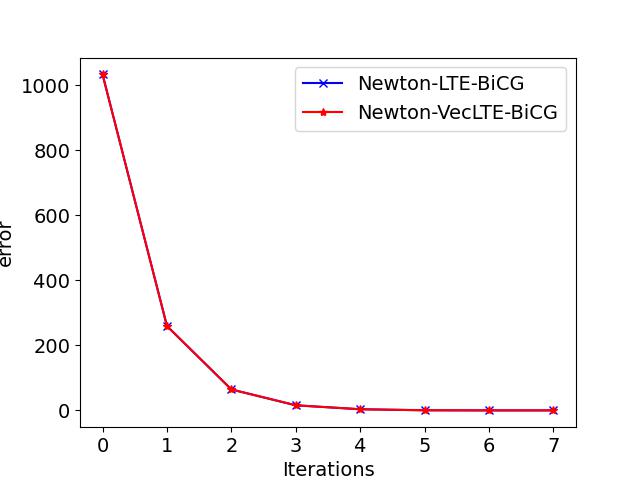
(a) residual error

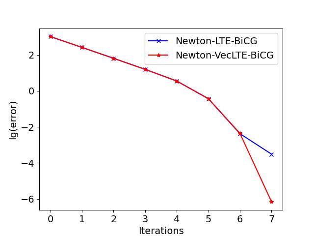
(b) logarithm of the residual error

Figure 1: Residual errors

The numerical solution $\mathcal{E}\in\mathbb{C}^{3\times 3\times 2\times 2}$ is obtained as given below, its approximate error is about $\|f(\mathcal{E})\|_{F}=6.9709\times 10^{-7}$. The smallest U-eigenvalue of $\mathcal{E}$ computed by the higher-order Rayleigh quotient iteration [5] is about $0.0063$, thus, $\mathcal{E}$ is positive definite. The U-eigenvalues of $\mathcal{A}-\mathcal{G}*\mathcal{E}$ are $-1.0165\pm 0.1846\iota$, $-0.4144\pm 0.4918\iota$ and $-0.0485\pm 0.3339\iota$, where $\iota=\sqrt{-1}$. Hence $\mathcal{A}-\mathcal{G}*\mathcal{E}$ is stable.

$$\begin{cases}\mathcal{E}_{::11}=\begin{bmatrix}4.8082&-0.2001&3.9671\\ -0.2001&1.5958&-3.3882\\ 3.9671&-3.3882&18.7381\end{bmatrix},\mathcal{E}_{::21}=\begin{bmatrix}-0.5391&-0.0033&1.5582\\ 10.0971&-4.2223&25.4769\\ 1.1050&0.0067&5.4633\end{bmatrix},\\ \mathcal{E}_{::12}=\begin{bmatrix}-0.5391&10.0971&1.1050\\ -0.0033&-4.2223&0.0067\\ 1.5582&25.4769&5.4633\end{bmatrix},\mathcal{E}_{::22}=\begin{bmatrix}0.9711&0.4996&0.7895\\ 0.4996&41.7634&6.7580\\ 0.7895&6.7580&2.9588\end{bmatrix}.\end{cases}$$

Furthermore, we compute the upper bounds according to Theorem 4.11 and Remark 4.15 for the condition numbers, we get $\kappa_{1}\lesssim 55.0299$, $\kappa_{2}\lesssim 75.4538$, and $\kappa_{3}\lesssim 123.7297$. To check these theoretical upper bounds, we conduct the numerical test by randomly setting the perturbations on coefficient tensors. Concretely, $\Delta\mathcal{A}=\gamma\frac{\|\mathcal{A}\|_{F}}{\|\Delta\tilde{\mathcal{A}}\|_{F}}\Delta\tilde{\mathcal{A}}$ where the elements of $\Delta\tilde{\mathcal{A}}$ are independently identically distributed in the standard normal distribution. For the perturbations of $\mathcal{G}$ and $\mathcal{K}$, we add the perturbation only on their nonzero entries, that is, $\Delta\mathcal{G}$ has only one nonzero entry with $\Delta\mathcal{G}_{1111}=\delta$, and the perturbation $\Delta\mathcal{K}$ has only one nonzero entry with $\Delta\mathcal{K}_{3322}=\delta$.

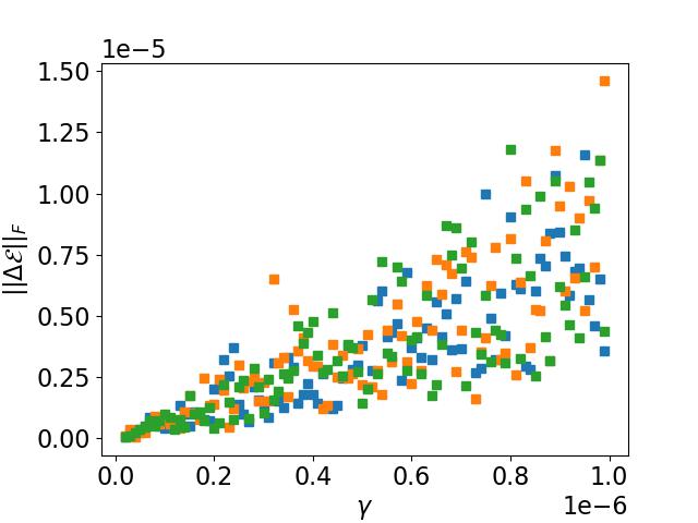
(a) The values of $\|\Delta\mathcal{E}\|_{F}$

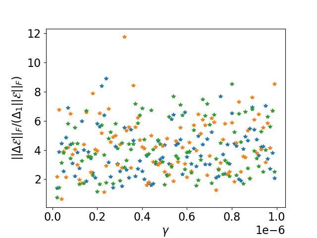
(b) The values of $\frac{\|\Delta\mathcal{E}\|_{F}}{\Delta_{1}\|\mathcal{E}\|_{F}}$

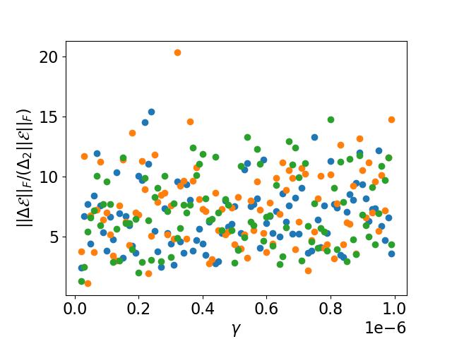
(c) The values of $\frac{\|\Delta\mathcal{E}\|_{F}}{\Delta_{2}\|\mathcal{E}\|_{F}}$

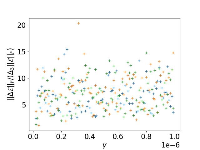
(d) The values of $\frac{\|\Delta\mathcal{E}\|_{F}}{\Delta_{3}\|\mathcal{E}\|_{F}}$

Figure 2: Perturbation errors. The randomized experiments for various perturbation factors $\delta=1\times 10^{-8}j\ (j=1,\cdots,99)$ are repeated three times, and the numerical results of the three independent experiments are presented in different colors in the four figures.

We perform randomized experiments independently for $\delta=1\times 10^{-8}j\ (j=1,\cdots,99)$ three times. The Frobenius norms $\|\Delta\mathcal{E}\|_{F}$ are shown in Figure 2 (a), and Figure 2 (b), (c) and (d) present the magnitudes of $\frac{\|\Delta\mathcal{E}\|_{F}}{\Delta_{1}\|\mathcal{E}\|_{F}}$, $\frac{\|\Delta\mathcal{E}\|_{F}}{\Delta_{2}\|\mathcal{E}\|_{F}}$ and $\frac{\|\Delta\mathcal{E}\|_{F}}{\Delta_{3}\|\mathcal{E}\|_{F}}$ respectively. It can be seen that they are all smaller than their theoretical upper bounds given above. Table 1 shows the relative errors $\frac{\|\Delta\mathcal{E}\|_{F}}{\|\mathcal{E}\|_{F}}$ and the estimates by these condition numbers under three different perturbation tests. Clearly, they all provide valid estimations.

Table 1: Comparison of the relative error $\frac{\|\Delta\mathcal{E}\|_{F}}{\|\mathcal{E}\|_{F}}$ with the estimates via condition numbers

$\delta$	$\|\Delta\mathcal{E}\|_{F}/\|\mathcal{E}\|_{F}$	$\kappa_{1}\Delta_{1}$	$\kappa_{2}\Delta_{2}$	$\kappa_{3}\Delta_{3}$
$1\times 10^{-8}$	$4.0547\times 10^{-8}$	$9.5314\times 10^{-7}$	$7.5453\times 10^{-7}$	$1.2373\times 10^{-6}$
$2\times 10^{-7}$	$2.2174\times 10^{-6}$	$1.9062\times 10^{-5}$	$1.5090\times 10^{-5}$	$2.4747\times 10^{-5}$
$3\times 10^{-6}$	$3.4478\times 10^{-5}$	$2.8594\times 10^{-4}$	$2.2636\times 10^{-4}$	$3.7121\times 10^{-4}$

6 Conclusion

In this paper, we have investigated in-depth even-order paired tensors under the Einstein product. For this class of tensors, we have defined Hamiltonian tensors and symplectic tensors and studied their structural decompositions and properties. We have applied these tensor computations to a class of continuous-time multilinear time-invariant control systems and studied a Lyapunov tensor equation. In particular, we have conducted a comprehensive study of an algebraic Riccati tensor equation (ARTE) and employed it to derive a tensor version of the bounded real lemma. In the future work, we are interested in developing more efficient numerical algorithms for solving this class of ARTEs. Another important research direction is to extend the current research to robust control of multilinear control systems. In particular, as complementary to well developed gain theory, a new phase theory has recently been proposed for linear control systems; see for example [35, 46]. It would be interesting to see whether phases can be defined for tensors and a useful phase theory can be developed for multilinear control systems.

Appendix A Additional tensor basics

Definition A.1 (Mode product [29]).

The mode-$n$ product of $\mathcal{X}\in\mathbb{C}^{I_{1}\times I_{2}\times\cdots\times I_{N}}$ and a matrix $A\in\mathbb{C}^{J_{n}\times I_{n}}$ is an $I_{1}\times\cdots\times I_{n-1}\times J_{n}\times I_{n+1}\times\cdots\times I_{N}$ tensor, given by

$$\left(\mathcal{X}\times_{n}A\right)_{i_{1}\cdots i_{n-1}ji_{n}\cdots i_{N}}=\sum_{i_{n}=1}^{I_{n}}\mathcal{X}_{i_{1}\cdots i_{n-1}i_{n}i_{n+1}\cdots i_{N}}A_{ji_{n}}.$$

There is a natural connection between even-order paired tensors and matrix outer products. For example, the tensor $\mathcal{A}=A_{1}\circ A_{2}\in\mathbb{C}^{I_{1}\times J_{1}\times I_{2}\times J_{2}}$ formed by the outer product of two matrices $A_{1}\in\mathbb{C}^{I_{1}\times J_{1}}$ and $A_{2}\in\mathbb{C}^{I_{2}\times J_{2}}$ is a fourth-order paired tensor. In fact, by viewing each paired indices as one long index, several classical tensor decompositions such as CANDECOMP/PARAFAC decomposition (CPD) [22] and the tensor-train decomposition [39] are naturally generalized to even-order paired tensors. Here, we only present the generalized CPD as it is used in Section 3.2 and the example in Section 5.

Definition A.2 (Generalized CPD [8]).

Let $\mathcal{A}\in\mathbb{C}^{I_{1}\times J_{1}\times\cdots\times I_{N}\times J_{N}}$ be an even-order paired tensor. Then $\mathcal{A}$ can be decomposed into a sum of a series of matrix outer products, i.e.,

(33) $$\mathcal{A}=\sum_{r=1}^{R}\mathcal{A}_{r::}^{(1)}\circ\mathcal{A}_{r::}^{(2)}\circ\cdots\circ\mathcal{A}_{r::}^{(N)},$$

where $\mathcal{A}^{(n)}\in\mathbb{C}^{R\times I_{n}\times J_{n}}$ for $n=1,\dots,N$. The smallest $R$ such that the above equation holds is called the CP rank of $\mathcal{A}$. In the article, the term ‘rank’ of a tensor always refers to the CP rank, if not otherwise specified.

Given two even-order paired tensors in the generalized CPD format, their Einstein product can be computed while preserving the structure, thus significantly reducing the computational cost compared to the computation by forming full tensors or tensor matrixization.

Proposition A.3 ([8]).

Given even-order paired tensors $\mathcal{A}\in\mathbb{C}^{I_{1}\times J_{1}\times\cdots\times I_{N}\times J_{N}}$ and $\mathcal{B}\in\mathbb{C}^{J_{1}\times K_{1}\times\cdots\times J_{N}\times K_{N}}$ in the generalized CPD format of (33) with ranks $R$ and $S$, respectively, the Einstein product $\mathcal{A}*\mathcal{B}$ can be computed in an economic fashion as $\mathcal{A}*\mathcal{B}=\sum_{t=1}^{T}\mathcal{F}_{t::}^{(1)}\circ\mathcal{F}_{t::}^{(2)}\circ\cdots\circ\mathcal{F}_{t::}^{(N)}$, where $\mathcal{F}_{t::}^{n}=\mathcal{A}_{r::}^{(n)}\mathcal{B}_{s::}^{(n)}\in\mathbb{C}^{I_{n}\times K_{n}}$ with $t=\mathrm{ivec}(\{r,s\},\{R,S\})$, and $T=RS$.

The following result can be easily established, so we omit its proof.

Proposition A.4.

For a rank-one even-order paired tensor $\mathcal{A}=A_{1}\circ A_{2}\circ\cdots\circ A_{N}\in\mathbb{C}^{I_{1}\times J_{1}\times\cdots\times I_{N}\times J_{N}}$,

1. $\mathcal{A}^{\rm H}=A_{1}^{\rm H}\circ A_{2}^{\rm H}\circ\cdots\circ A_{N}^{\rm H}$;

2. if $A_{n}\ (n=1,\dots,N)$ are upper-triangular matrices, then $\mathcal{A}$ is an upper-triangular even-order paired tensor;

3. if $A_{n}\ (n=1,\dots,N)$ are unitary matrices, then $\mathcal{A}$ is a unitary tensor;

4. if $A_{n}\ (n=1,\dots,N)$ are invertible, then $\mathcal{A}$ is also invertible, and $\mathcal{A}^{\rm-1}=A_{1}^{-1}\circ A_{2}^{\rm-1}\circ\cdots\circ A_{N}^{\rm-1}$.

Appendix B Proofs

The proof of Proposition 3.12. We prove these properties one by one. Property 1 can be easily obtained via tensor matrixization and [43, Theorem 3.3]. For Property 2, firstly, $(\mathcal{A}\otimes\mathcal{B})^{\mathrm{H}}\in\mathbb{C}^{J_{1}L_{1}\times I_{1}K_{1}\times\cdots\times J_{N}L_{N}\times I_{N}K_{N}}$. Then from Definition 3.10 of tensor Kronecker product, for all $\mathbf{1}\leq\mathbf{i}\leq\mathbf{I},\mathbf{1}\leq\mathbf{j}\leq\mathbf{J}$, it follows that

$$\left((\mathcal{A}\otimes\mathcal{B})^{\mathrm{H}}\right)_{[\mathbf{j}\wedge\mathbf{i}]} =(\mathcal{A}\otimes\mathcal{B})^{\mathrm{H}}((j_{1}-1)L_{1}+1:j_{1}L_{1},(i_{1}-1)K_{1}+1:i_{1}K_{1},\cdots,$$

$$\quad\quad\quad\quad\quad\ \ (j_{N}-1)L_{N}+1:j_{N}L_{N},(i_{N}-1)K_{N}+1:i_{N}K_{N})$$

$$=\overline{\mathcal{A}_{i_{1}j_{1}\cdots i_{N}j_{N}}}\cdot\mathcal{B}^{\mathrm{H}}=(\mathcal{A}^{\mathrm{H}})_{j_{1}i_{1}\cdots j_{N}i_{N}}\cdot\mathcal{B}^{\mathrm{H}},$$

which shows that $(\mathcal{A}\otimes\mathcal{B})^{\mathrm{H}}$ is the Kronecker product of $\mathcal{A}^{\mathrm{H}}$ and $\mathcal{B}^{\mathrm{H}}$. Next, we prove Property 3. The tensor $(\mathcal{A}\otimes\mathcal{B})*(\mathcal{C}\otimes\mathcal{D})$ is an $I_{1}\times R_{1}\times\cdots\times I_{N}\times R_{N}$ block tensor. For $\mathbf{1}\leq\mathbf{i}\leq\mathbf{I}$, $\mathbf{1}\leq\mathbf{r}\leq\mathbf{R}$, the $(\mathbf{i}\wedge\mathbf{r})$th block of $(\mathcal{A}\otimes\mathcal{B})*(\mathcal{C}\otimes\mathcal{D})$ is

$$\left((\mathcal{A}\otimes\mathcal{B})*(\mathcal{C}\otimes\mathcal{D})\right)_{[\mathbf{i}\wedge\mathbf{r}]}$$

$$\ =\sum_{\mathbf{1}\leq\mathbf{j}\leq\mathbf{J}}(\mathcal{A}\otimes\mathcal{B})_{[\mathbf{i}\wedge\mathbf{j}]}*(\mathcal{C}\otimes\mathcal{D})_{[\mathbf{j}\wedge\mathbf{r}]}=\sum_{\mathbf{1}\leq\mathbf{j}\leq\mathbf{J}}(\mathcal{A}_{i_{1}j_{1}\cdots i_{N}j_{N}}\cdot\mathcal{B})*(\mathcal{C}_{j_{1}r_{1}\cdots j_{N}r_{N}}\cdot\mathcal{D})$$

$$\ =\mathcal{B}*\mathcal{D}\sum_{\mathbf{1}\leq\mathbf{j}\leq\mathbf{J}}\mathcal{A}_{i_{1}j_{1}\cdots i_{N}j_{N}}\mathcal{C}_{j_{1}r_{1}\cdots j_{N}r_{N}}=(\mathcal{A}*\mathcal{C})_{i_{1}r_{1}\cdots i_{N}r_{N}}\cdot(\mathcal{B}*\mathcal{D})$$

$$\ =\left((\mathcal{A}*\mathcal{C})\otimes(\mathcal{B}*\mathcal{D})\right)_{[\mathbf{i}\wedge\mathbf{r}]}.$$

Thus, $(\mathcal{A}\otimes\mathcal{B})*(\mathcal{C}\otimes\mathcal{D})=(\mathcal{A}*\mathcal{C})\otimes(\mathcal{B}*\mathcal{D})$. Property 4 follows from Property 3. $\Box$

The proof of Proposition 3.21. We know that both $\mathrm{Vec}(\mathcal{U}*\mathcal{X}*\mathcal{W})$ and $(\mathcal{W}^{\top}\otimes\mathcal{U})*\mathrm{Vec}(\mathcal{X})\in\mathbb{C}^{L_{1}I_{1}\times\cdots\times L_{N}I_{N}}$ are $L_{1}\times\cdots\times L_{N}$ block tensors, each subblock is of size $I_{1}\times\cdots\times I_{N}$. Hence, it suffices to compare all subblock tensors. For $\mathbf{l}=(l_{1},\dots,l_{N})$, the $\mathbf{l}$-th subblock $\mathrm{Vec}(\mathcal{U}*\mathcal{X}*\mathcal{W})_{[\mathbf{l}]}=\left(\mathcal{U}*\mathcal{X}*\mathcal{W}\right)_{:l_{1},\cdots,:l_{N}}=\mathcal{U}*\mathcal{X}*\mathcal{W}_{:l_{1},\cdots,:l_{N}}$, and $\left((\mathcal{W}^{\top}\otimes\mathcal{U})*\mathrm{Vec}(\mathcal{X})\right)_{[\mathbf{l}]}=\sum_{\mathbf{1}\leq\mathbf{k}\leq\mathbf{K}}(\mathcal{W}^{\top}\otimes\mathcal{U})_{[\mathbf{l}\wedge\mathbf{k}]}*\mathrm{Vec}(\mathcal{X})_{[\mathbf{k}]}=\sum_{\mathbf{1}\leq\mathbf{k}\leq\mathbf{K}}\mathcal{W}_{k_{1}l_{1}\cdots k_{N}l_{N}}\mathcal{U}*\mathcal{X}_{:k_{1},\cdots,:k_{N}}=\mathcal{U}*\mathcal{X}*\mathcal{W}_{:l_{1},\cdots,:l_{N}}$. Thereby, the result holds.

Appendix C Fast operations for structured tensors

The following result can be easily checked.

Proposition C.1.

Given $\mathcal{E}\in\mathbb{C}^{I_{1}\times J_{1}\times\cdots\times I_{N}\times J_{N}}$ and a rank-one tensor $\mathcal{A}=A_{1}\circ\cdots\circ A_{N}$, we have

1. $\mathcal{E}*\mathcal{A}=\mathcal{E}\times_{2}A_{1}^{\top}\times_{4}A_{2}^{\top}\times_{6}\cdots\times_{2N}A_{N}^{\top}$ if $A_{n}\in\mathbb{C}^{J_{n}\times K_{n}}$;

2. $\mathcal{A}*\mathcal{E}=\mathcal{E}\times_{1}A_{1}\times_{3}A_{2}\times_{5}\cdots\times_{2N-1}A_{N}$ if $A_{n}\in\mathbb{C}^{K_{n}\times I_{n}}$.

Remark C.2.

It requires $O\left((|\mathbf{I}|+N-1)|\mathbf{J}||\mathbf{K}|\right)$ multiplications for the above Einstein product $\mathcal{E}*\mathcal{A}$ based on full tensor or tensor matrixization, but only needs $O\left(|\mathbf{I}||\mathbf{J}|(\sum_{n=1}^{N}\frac{K_{1}\cdots K_{n-1}K_{n}}{J_{1}\cdots J_{n-1}})\right)$ multiplications according to the decompositions shown in Proposition C.1, thus saving a lot of computational and storage costs.

Remark C.3.

From Propositions C.1 and A.4, the ARTE (4) reduces to the Lyapunov tensor equation $\mathcal{E}\times_{1}A+\mathcal{E}\times_{2}A+\cdots+\mathcal{E}\times_{2N}A+\mathcal{K}=\mathcal{O}$ with $A\in\mathbb{R}^{m\times m}$, if $\mathcal{G}=\mathcal{O}$ and

(34) $$\mathcal{A}=A^{\top}\circ I_{m}\circ\cdots\circ I_{m}+I_{m}\circ A^{\top}\circ\cdots\circ I_{m}+\cdots+I_{m}\circ\cdots\circ I_{m}\circ A^{\top}$$

Proposition C.4.

Let $\mathcal{A}\in\mathbb{C}^{m\times m\times\cdots\times m\times m}$ be the $2N$th-order paired tensor as given in (34), and the eigenvalues of $A$ are $\{\lambda_{1},\lambda_{2},\dots,\lambda_{m}\}$. Then the U-eigenvalues of $\mathcal{A}$ are $\Lambda(\mathcal{A})=\{\lambda_{i_{1}}+\cdots+\lambda_{i_{N}}\big{|}i_{n}=1,\dots,m\ \mathrm{for}\ \mathrm{all}\ n=1,\dots,N\}$.

Proof C.5.

Let the Schur decomposition of the matrix $A^{\top}$ be $A^{\top}=URU^{\rm H}$, where $U\in\mathbb{C}^{m\times m}$ is a unitary matrix, and $R\in\mathbb{C}^{m\times m}$ is an upper-triangular matrix whose diagonal entries $R_{kk}=\lambda_{k},k=1,\dots,m$. For all $n=1,\dots,N$ and the rank-one tensor $\mathcal{A}_{n}=\underbrace{I_{m}\circ\cdots\circ I_{m}}_{n-1\ \mathrm{terms}}\circ A^{\top}\circ\underbrace{I_{m}\circ\cdots\circ I_{m}}_{N-n\ \mathrm{terms}}$, it follows from Propositions A.3 and A.4 that $\mathcal{A}_{n}=\left(UI_{m}U^{\rm H}\right)\circ\cdots\circ\left(UI_{m}U^{\rm H}\right)\circ\left(URU^{\rm H}\right)\circ\left(UI_{m}U^{\rm H}\right)\circ\cdots\circ\left(UI_{m}U^{\rm H}\right)=\mathcal{U}*\mathcal{R}_{n}*\mathcal{U}^{\rm H}$, where $\mathcal{U}=U\circ U\circ\cdots\circ U\in\mathbb{C}^{m\times m\times\cdots\times m\times m}$ is a unitary tensor, and $\mathcal{R}_{n}=I_{m}\circ\cdots\circ I_{m}\circ R\circ I_{m}\circ\cdots\circ I_{m}$ is an upper-triangular $2N$th-order paired tensor. Hence, $\mathcal{A}=\mathcal{U}*\mathcal{R}*\mathcal{U}^{\rm H}$ with $\mathcal{R}=\left(\mathcal{R}_{1}+\cdots+\mathcal{R}_{N}\right)$ is the tensor Schur decomposition of $\mathcal{A}$. According to Lemma 2.12, the diagonal entries of $\mathcal{R}$ are the U-eigenvalues of $\mathcal{A}$. From the definition of the outer product, the diagonal elements, i.e., the U-eigenvalues of $\mathcal{A}$ are $\mathcal{R}_{i_{1}i_{1}\cdots i_{N}i_{N}}=(\mathcal{R}_{1})_{i_{1}i_{1}\cdots i_{N}i_{N}}+\cdots+(\mathcal{R}_{N})_{i_{1}i_{1}\cdots i_{N}i_{N}}=R_{i_{1}i_{1}}+R_{i_{2}i_{2}}+\cdots+R_{i_{N}i_{N}}=\lambda_{i_{1}}+\lambda_{i_{2}}+\cdots+\lambda_{i_{N}}$ for all $i_{n}=1,\dots,m$ and $n=1,\dots,N$.

Remark C.6.

According to Proposition C.4, the tensor $\mathcal{A}$ in (34) is stable if and only if the matrix $A$ is stable.

For rank-one even-order paired tensors, the following results can be easily established, therefore their proofs are omitted.

Proposition C.7 (Schur decomposition).

Let $\mathcal{A}=A_{1}\circ A_{2}\circ\cdots\circ A_{N}$ be a rank-one even-order paired tensor, where $A_{k}\in\mathbb{C}^{I_{k}\times I_{k}}$. Given the Schur decompositions $A_{n}=U_{n}R_{n}U_{n}^{\rm H}$ for all $n=1,\dots,N$, the tensor Schur decomposition of $\mathcal{A}$ is $\mathcal{A}=\mathcal{U}*\mathcal{R}*\mathcal{U}^{\rm H}$, where $\mathcal{U}=U_{1}\circ U_{2}\circ\cdots\circ U_{N}$ is unitary, and $\mathcal{R}=R_{1}\circ R_{2}\circ\cdots\circ R_{N}$ is upper-triangular. Therefore, the U-eigenvalues of $\mathcal{A}$ are the products of the eigenvalues of $A_{n}\ (n=1,\dots,N)$, i.e., $\Lambda(\mathcal{A})=\{\prod_{n=1}^{N}\lambda_{n}\big{|}\ \lambda_{n}\in\Lambda(A_{n})\}$.

Proposition C.8.

For the rank-one even-order paired tensor $\mathcal{A}=A_{1}\circ\cdots\circ A_{N}$, $\|\mathcal{A}\|_{\star}={\textstyle\prod_{n=1}^{N}}\|A_{n}\|_{\star}$, where $\star$ denotes either the Frobenius norm or the spectral norm.

Proposition C.9.

$\|\mathcal{A}\otimes\mathcal{B}\|_{\star}=\|\mathcal{A}\|_{\star}\|\mathcal{B}\|_{\star}$, where $\star$ denotes either the Frobenius norm or the spectral norm.

References

- [1] F. P. Ali Beik, F. S. Movahed, and S. Ahmadi-Asl, On the Krylov subspace methods based on tensor format for positive definite Sylvester tensor equations, Numerical Linear Algebra with Applications, 23 (2016), pp. 444–466.
- [2] M. Bai, J. Chen, Q. Zhao, C. Li, J. Zhang, and J. Gao, Tensor neural controlled differential equations, in 2022 International Joint Conference on Neural Networks (IJCNN), IEEE, 2022, pp. 1–9.
- [3] M. Bai, Q. Zhao, and J. Gao, Tensorial time series prediction via tensor neural ordinary differential equations, in 2021 International Joint Conference on Neural Networks (IJCNN), IEEE, 2021, pp. 1–8.
- [4] S. Boyd, V. Balakrishnan, and P. Kabamba, A bisection method for computing the norm of a transfer matrix and related problems, Mathematics of Control, Signals and Systems, 2 (1989), pp. 207–219.
- [5] M. Brazell, N. Li, C. Navasca, and C. Tamon, Solving multilinear systems via tensor inversion, SIAM Journal on Matrix Analysis and Applications, 34 (2013), pp. 542–570.
- [6] S. Y. Chang and H.-C. Wu, Multi-relational data characterization by tensors: Tensor inversion, IEEE Transactions on Big Data, 8 (2021), pp. 1650–1663.
- [7] C. Chen, A. Surana, A. Bloch, and I. Rajapakse, Multilinear time invariant system theory, in 2019 Proceedings of the Conference on Control and its Applications, SIAM, 2019, pp. 118–125.
- [8] C. Chen, A. Surana, A. M. Bloch, and I. Rajapakse, Multilinear control systems theory, SIAM Journal on Control and Optimization, 59 (2021), pp. 749–776.
- [9] A. Cichocki, R. Zdunek, A. H. Phan, and S.-i. Amari, Nonnegative Matrix and Tensor Factorizations: Applications to Exploratory Multi-way Data Analysis and Blind Source Separation, NewYork: Wiley, 2009.
- [10] L.-B. Cui, C. Chen, W. Li, and M. K. Ng, An eigenvalue problem for even order tensors with its applications, Linear and Multilinear Algebra, 64 (2016), pp. 602–621.
- [11] S. Cui, Q. Zhao, H. Jardon-Kojakhmetov, and M. Cao, Species coexistence and extinction resulting from higher-order Lotka-Volterra two-faction competition, in 2023 62nd IEEE Conference on Decision and Control (CDC), IEEE, 2023, pp. 467–472.
- [12] G. Daniel and J. Gray, Opt_einsum-a Python package for optimizing contraction order for einsum-like expressions, Journal of Open Source Software, 3 (2018), p. 753.
- [13] W. Ding, K. Liu, E. Belyaev, and F. Cheng, Tensor-based linear dynamical systems for action recognition from 3D skeletons, Pattern Recognition, 77 (2018), pp. 75–86.
- [14] G. A. Dotson, C. Chen, S. Lindsly, A. Cicalo, S. Dilworth, C. Ryan, S. Jeyarajan, W. Meixner, C. Stansbury, J. Pickard, et al., Deciphering multi-way interactions in the human genome, Nature Communications, 13 (2022), p. 5498.
- [15] A. Einstein, The foundation of the general theory of relativity, Annalen Phys, 49 (1916), pp. 769–822.
- [16] M. El Guide, A. El Ichi, K. Jbilou, and F. Beik, Tensor Krylov subspace methods via the Einstein product with applications to image and video processing, Applied Numerical Mathematics, 181 (2022), pp. 347–363.
- [17] S. El-Halouy, S. Noschese, and L. Reichel, A tensor formalism for multilayer network centrality measures using the Einstein product, Applied Numerical Mathematics, (2023).
- [18] A. R. Ghavimi and A. J. Laub, Backward error, sensitivity, and refinement of computed solutions of algebraic Riccati equations, Numerical linear algebra with applications, 2 (1995), pp. 29–49.
- [19] G. H. Golub and C. F. Van Loan, Matrix Computations, Johns Hopkins University Press, Baltimore, MD, 4th ed., 2013.
- [20] A. Graham, Kronecker Products and Matrix Calculus with Applications, Courier Dover Publications, 2018.
- [21] M. Hajarian, Conjugate gradient-like methods for solving general tensor equation with Einstein product, Journal of the Franklin Institute, 357 (2020), pp. 4272–4285.
- [22] F. L. Hitchcock, The expression of a tensor or a polyadic as a sum of products, Journal of Mathematics and Physics, 6 (1927), pp. 164–189.
- [23] B. Huang, Y. Xie, and C. Ma, Krylov subspace methods to solve a class of tensor equations via the Einstein product, Numerical Linear Algebra with Applications, 26 (2019), p. e2254.
- [24] Z.-H. Huang and L. Qi, Positive definiteness of paired symmetric tensors and elasticity tensors, Journal of Computational and Applied Mathematics, 338 (2018), pp. 22–43.
- [25] M. Itskov, On the theory of fourth-order tensors and their applications in computational mechanics, Computer Methods in Applied Mechanics and Engineering, 189 (2000), pp. 419–438.
- [26] C. T. Kelley, Solving Nonlinear Equations with Newton’s Method, SIAM, 2003.
- [27] S. Kesavan, Nonlinear Functional Analysis: A First Course, vol. 28, Springer Nature, 2022.
- [28] H. Kimura, Chain-scattering Approach to Control, Springer Science & Business Media, 1996.
- [29] T. G. Kolda and B. W. Bader, Tensor decompositions and applications, SIAM Review, 51 (2009), pp. 455–500.
- [30] P. Lancaster and L. Rodman, Algebraic Riccati Equations, Clarendon press, 1995.
- [31] A. D. Letten and D. B. Stouffer, The mechanistic basis for higher-order interactions and non-additivity in competitive communities, Ecology Letters, 22 (2019), pp. 423–436.
- [32] M. Liang, B. Zheng, and R. Zhao, Tensor inversion and its application to the tensor equations with Einstein product, Linear and Multilinear Algebra, 67 (2019), pp. 843–870.
- [33] H. Lu, K. N. Plataniotis, and A. Venetsanopoulos, Multilinear subspace learning: dimensionality reduction of multidimensional data, CRC press, 2013.
- [34] H. Ma, N. Li, P. S. Stanimirović, and V. N. Katsikis, Perturbation theory for Moore–Penrose inverse of tensor via Einstein product, Computational and Applied Mathematics, 38 (2019), p. article III.
- [35] X. Mao, W. Chen, and L. Qiu, Phases of discrete-time LTI multivariable systems, Automatica, 142 (2022), p. 110311.
- [36] M. M. Mehrabadi and S. C. Cowin, Eigentensors of linear anisotropic elastic materials, The Quarterly Journal of Mechanics and Applied Mathematics, 43 (1990), pp. 15–41.
- [37] J. Nie, Moment and Polynomial Optimization, SIAM, 2023.
- [38] R. Orús, Tensor networks for complex quantum systems, Nature Reviews Physics, 1 (2019), pp. 538–550.
- [39] I. V. Oseledets, Tensor-train decomposition, SIAM Journal on Scientific Computing, 33 (2011), pp. 2295–2317.
- [40] C. Paige and C. Van Loan, A Schur decomposition for Hamiltonian matrices, Linear Algebra and its applications, 41 (1981), pp. 11–32.
- [41] J. Pickard, C. Stansbury, C. Chen, A. Surana, A. Bloch, and I. Rajapakse, Kronecker product of tensors and hypergraphs, arXiv preprint arXiv:2305.03875, (2023).
- [42] L. Qi, H. Chen, and Y. Chen, Tensor Eigenvalues and Their Applications, vol. 39, Springer, 2018.
- [43] S. Ragnarsson and C. F. Van Loan, Block tensor unfoldings, SIAM Journal on Matrix Analysis and Applications, 33 (2012), pp. 149–169.
- [44] J. R. Rice, A theory of condition, SIAM Journal on Numerical Analysis, 3 (1966), pp. 287–310.
- [45] M. Rogers, L. Li, and S. J. Russell, Multilinear dynamical systems for tensor time series, Advances in Neural Information Processing Systems, 26 (2013), pp. 2634–2642.
- [46] R. Srazhidinov, D. Zhang, and L. Qiu, Computation of the phase and gain margins of MIMO control systems, Automatica, 149 (2023), p. 110846.
- [47] A. Surana, G. Patterson, and I. Rajapakse, Dynamic tensor time series modeling and analysis, in 2016 IEEE 55th Conference on Decision and Control (CDC), IEEE, 2016, pp. 1637–1642.
- [48] Y. Wang and Y. Wei, Generalized eigenvalue for even order tensors via Einstein product and its applications in multilinear control systems, Computational and Applied Mathematics, 41 (2022), p. 419.
- [49] G. Zhang and Z. Dong, Linear quantum systems: A tutorial, Annual Reviews in Control, 54 (2022), pp. 274–294.
- [50] K. Zhou and J. C. Doyle, Essentials of Robust Control, vol. 104, Prentice hall Upper Saddle River, NJ, 1998.
- [51] L. Zhou, Y. Lin, Y. Wei, and S. Qiao, Perturbation analysis and condition numbers of symmetric algebraic Riccati equations, Automatica, 45 (2009), pp. 1005–1011.