Generalized linear models with spatial dependence and a functional covariate

Abstract

[Abstract] We extend generalized functional linear models under independence to a situation in which a functional covariate is related to a scalar response variable that exhibits spatial dependence. For estimation, we apply basis expansion and truncation for dimension reduction of the covariate process followed by a composite likelihood estimating equation to handle the spatial dependency. We develop asymptotic results for the proposed model under a repeating lattice asymptotic context, allowing us to construct a confidence interval for the spatial dependence parameter and a confidence band for the parameter function. A binary conditionals model is presented as a concrete illustration and is used in simulation studies to verify the applicability of the asymptotic inferential results.

1 Introduction

In recent years, functional data analysis (FDA) has seen rapid development; see, for example, ¹⁸, ¹³, ⁷, and ⁶. In FDA, there are three types of regression; scalar-on-function regression, function-on-scalar regression, and function-on-function regression. Our interest here is in generalized functional linear regression models with a functional covariate and a real-valued response. Previous work on generalized functional linear regression includes ⁹, ¹⁰, ¹⁶, ³, and ⁴. A challenge in handling functional data is the infinite dimensionality. In particular, ¹⁶ tackled this in their generalized functional linear regression model using a truncation strategy for dimension reduction of the covariate process.

Functional data that contain spatial structure have also been considered, where a recent review is ¹⁵. Much focus has been on extending the concept of functions as datum to situations in which an entire continuous spatial field is treated as a datum.

In this article, we are primarily interested in functional generalized linear models for real-valued lattice, or areal response variables that exhibit spatial dependence, that depends on a functional covariate. ¹⁴ proposed practical modeling for spatial lattice correlated data using a generalized estimating equation with Moran’s index. They considered the spatial dependence but did not have a functional covariate and did not investigate asymptotic properties. ²⁰ studied asymptotic theory for generalized estimating equations analysis of binary response with high-dimensional covariates, rather than a functional covariate. ⁸ suggested a generalized functional linear model for a functional covariate and real-valued longitudinal responses that exhibit dependence over time. These authors deal with dependence in response variables using a generalized estimating equation and used some assumptions from ²⁰, but one of the assumptions fails to hold for functional data because the basis coefficients must decay to 0 in this situation. We apply an alternative condition and provide a new proof in this work. To the best of our knowledge, there is no literature concerning spatial functional generalized linear models where responses given covariates follow (conditional) exponential dispersion family distributions and the covariate processes are functional. Our goal is to introduce such models, present an estimation strategy that improves on previously used estimating equations, and provide asymptotic results. Our approach is built on a backbone of Markov random field models for spatially dependent responses and the truncation strategy of ¹⁶ applied to functional covariates.

The rest of this article is organized as follows. In Section 2, we outline the background of the Markov random field approach and propose the spatial generalized linear model with a functional covariate. We present an estimation strategy using composite likelihood in Section 3, and give theoretical results in Section 4. Results from a simulation study are provided in Section 5, and we give some concluding remarks in Section 6. Proofs of the main theorems are given in an appendix and proofs of lemmas and propositions are in the Supplementary Materials.

2 Model

2.1 Markov random field

We begin this section with a brief overview of exponential family Markov random field models in the spatial context. Let $\mathbf{s}_{i}$ denote spatial locations on a finite index random field, for $i=1,\ldots,n$. For example, we may have $\mathbf{s}_{i}=(u_{i},v_{i})$, where $u_{i}$ denotes longitude, or a horizontal coordinate on a regular lattice, and $v_{i}$ denotes latitude or a vertical coordinate on a lattice. Let $\{Y(\mathbf{s}_{i}):i=1,\ldots,n\}$ be random variables indexed to the spatial locations and let $f$ be generic notation for a density (or mass) of a multivariate real-valued random variable such that $f(x)$ is the density of the random variable $X$, $f(y)$ is the density of the random variable $Y$, and so forth. Distributions of the $Y(\mathbf{s}_{i})$ are assigned as full conditional distributions, $f(y(\mathbf{s}_{i})|\{y(\mathbf{s}_{j}):\,j\neq i\})$. Now, for each location $\mathbf{s}_{i}$ define a neighborhood $N_{i}$ is as

$$N_{i}=\{\mathbf{s}_{k}:\,f(y(\mathbf{s}_{i})|\{y(\mathbf{s}_{j}):\,j\neq i\})\text{ depends functionally on }y(\mathbf{s}_{k})\text{ for }k\neq i\},$$

and let $\mathbf{y}(N_{i})=\{\mathbf{y}(\mathbf{s}_{j}):\,\mathbf{s}_{j}\in N_{i}\}$. The implication is the Markov assumption that,

$$f(y(\mathbf{s}_{i})|\{y(\mathbf{s}_{j}):\,j\neq i\})=f(y(\mathbf{s}_{i})|\mathbf{y}(N_{i})).$$

Typically, neighborhood structures are designated as a part of model formulation. Common examples of neighborhood structures on a regular lattice are the four-nearest neighborhood structure and the eight-nearest neighborhood structure. If $\mathbf{s}_{i}=(u_{i},v_{i})$ where $u_{i}$ and $v_{i}$ are horizontal and vertical coordinates, respectively, a four-nearest neighborhood is given as,

$$N_{4,i}=\{\mathbf{s}_{j}:\,\,(u_{j}=u_{i},v_{j}=v_{i}\pm 1)\text{ or }(u_{j}=u_{i}\pm 1,v_{j}=v_{i})\},$$

and an eight-nearest neighborhood is given as,

$$N_{i}=N_{4,i}\cup\{u_{j}=u_{i}\pm 1,\,v_{j}=v_{i}\pm 1\}.$$

Under suitable conditions, a joint distribution that corresponds to the full conditionals exists, and can be identified up to an unknown normalizing constant that depends on any parameters in the model, but not the response random variables. Details can be found in, for example, ¹².

Within the context of generalized linear models, the full conditional distributions in a Markov random field model are given as one-parameter exponential families,

$$f(y(\mathbf{s}_{i})|\mathbf{y}(N_{i}),\theta)=\exp\left[A_{i}(\mathbf{y}(N_{i})),\theta)y(\mathbf{s}_{i})-B_{i}(\mathbf{y}(N_{i}),\theta)+C(y(\mathbf{s}_{i}))\right]$$ (1)

where $A_{i}(\mathbf{y}(N_{i}))$ is a natural parameter function that depends on the neighboring values of $Y(\mathbf{s}_{i})$, and $B_{i}(\mathbf{y}(N_{i}))$ is a function of $A_{i}(\mathbf{y}(N_{i}))$ that determines the distributional form and moments. The function $C(\cdot)$ normalizes the distribution. Now let $\mathbf{\theta}$ denote any parameters that may appear in the specified form of the full conditional distributions. Under a few conditions, ¹ showed that the natural parameter function $A_{i}(\cdot)$ must satisfy $A_{i}(\mathbf{y}(N_{i}),\mathbf{\theta})=\alpha_{i}+\sum_{\mathbf{s}_{j}\in N_{i}}\eta_{i,j}y(\mathbf{s}_{j})$ where $\alpha_{i}$ is a leading constant and $\{\eta_{i,j}\}$ are dependence parameters satisfying $\eta_{i,j}=\eta_{j,i}$, $\eta_{i,i}=0$, and $\eta_{i,j}=0$ unless $\mathbf{s}_{j}\in N_{i}$. If external covariates influence the conditional distributions (1) they are incorporated into the leading term $\alpha_{i}$ using, for example, a standard link function from generalized linear models. To improve the interpretability of regression parameters in such a model, ¹¹ proposed to instead consider a centered parameterization, $A_{i}(y(\mathbf{s}_{i}),\mathbf{\theta})=\tau^{-1}(\kappa_{i})+\sum_{\mathbf{s}_{j}\in N_{i}}\eta_{i,j}\{y(\mathbf{s}_{j})-\kappa_{j}\}$, where $\tau^{-1}(\cdot)$ is a function that maps expected values into natural parameters, and $\kappa_{i}$ is the expected value of $Y(\mathbf{s}_{i})$ under an independence model. We also note that the model becomes degenerate if $\eta_{i,j}$ becomes too big.

2.2 Model

Let $\mathcal{L}_{2}(\mathcal{T})$ be the set of all square-integrable functions on a closed interval $\mathcal{T}$. Let $\{X_{i}(t),t\in\mathcal{T}\}$ be a functional covariate that takes values in $\mathcal{L}_{2}(\mathcal{T})$ with $\mu=EX_{i}(t)=0$ for $i\in\{1,\cdots,n\}$. We assume constant dependence, that is, $\eta_{i,j}=\eta$ for all $i$ and $j$. A spatial generalized linear model with functional covariates and real-valued responses $y(\mathbf{s}_{i})$ is then, for $i=1,\ldots,n$,

$$\begin{split}f(y(\mathbf{s}_{i})|\mathbf{y}(N_{i}),X_{i},\mathbf{\theta})&=\exp\left[A_{i}(\mathbf{y}(N_{i}),\mathbf{\theta})y(\mathbf{s}_{i})-B_{i}(\mathbf{y}(N_{i}),\mathbf{\theta})+C(y(\mathbf{s}_{i}))\right],\\ A_{i}(\mathbf{y}(N_{i}),\mathbf{\theta})&=\tau^{-1}(\kappa_{i})+\eta\sum_{\mathbf{s}_{j}\in N_{i}}\{y(\mathbf{s}_{j})-\kappa_{j}\},\\ B_{i}(\cdot,\mathbf{\theta})&\text{ is a function of }A_{i}(\cdot,\mathbf{\theta}),\\ g(\kappa_{i})&=\alpha+\int\beta(t)X_{i}(t)\,dt,\end{split}$$ (2)

where $\tau^{-1}(\cdot)$ is a function that maps expected values into natural parameters for the desired exponential family, $\eta$ is a dependence parameter, and $g(\cdot)$ is a link function that relates expectations under independence, $\kappa_{i}$, to a linear predictor with intercept parameter $\alpha$, and a parameter function $\beta(\cdot)$ which is assumed to be in $\mathcal{L}_{2}(\mathcal{T})$. The case in which $g(\kappa_{i})=\tau^{-1}(\kappa_{i})$ corresponds to a generalized linear model with canonical link. In this model, the large-scale structure of the spatial model for responses, namely the mean structure of independence model, is modeled via $\kappa_{i}$ through a functional covariate; and the small-scale structure, namely the spatial dependency, is modeled through the dependence parameter. Note that we have written the random model component in (2) without the common dispersion parameter in the generalized linear model. A separate dispersion parameter could be added when needed, such as for Gaussian or Inverse Gaussian random components. The most common non-Gaussian models in spatial applications are natural exponential families such as binary and (Winsorized) Poisson models for which the dispersion parameter can be taken as $1$.

Let $\{\phi_{j}\}_{j=1}^{\infty}$ be an orthonormal basis of the functional space $\mathcal{L}_{2}(\mathcal{T})$, for example, a trignometric basis. A basis expansion can be used for the functional covariate $X_{i}(t)$ and the parameter function $\beta(t)$ as

$$X_{i}(t)=\sum_{j=1}^{\infty}\varepsilon_{j}^{(i)}\phi_{j}(t),\quad\beta(t)=\sum_{j=1}^{\infty}\beta_{j}\phi_{j}(t)$$

where $\varepsilon_{j}^{(i)}=\int X_{i}(t)\phi_{j}(t)dt$ and $\beta_{j}=\int\beta(t)\phi_{j}(t)dt$. The implication is that

$$\int\beta(t)X_{i}(t)dt=\sum_{j=1}^{\infty}\beta_{j}\varepsilon_{j}^{(i)}.$$

From the basis expansion, the link function in the model (2) can be rewritten as

$$g(\kappa_{i}) =\alpha+\sum_{j=1}^{\infty}\beta_{j}\varepsilon_{j}^{(i)}.$$

We approximate the infinite sum using a truncated version at $p$ terms, following the truncation strategy introduced in ¹⁶. The $p$-truncated model is formed through a truncation of the basis expansion,

$$g(\kappa_{i}) =\alpha+\sum_{j=1}^{p}\beta_{j}\varepsilon_{j}^{(i)},$$

where $p$ diverges as the independent realizations or the sample size diverges depending on the asymptotic context. In the $p$-truncated model, we can consider the finite-dimensional parameter vector instead of a parameter function. The $p$-truncated model will be used for the estimation and asymptotic inference in Section 3 and Section 4, respectively.

We now give a specific example of Model (2) to make the concepts and notation more concrete, that being a binary conditionals model with functional covariate and canonical link. This model will also be used in the simulation study to follow.

Example 2.1 (Binary conditional model).

Suppose that we are interested in spatially dependent binary responses at locations $\{\mathbf{s}_{i}:\,i=1,\ldots,n\}$ with a functional covariate. Let $\{X_{i}(t):t\in\mathcal{T}\}$ be functional covariates. For $\mathbf{\theta}=(\eta,\alpha,\beta_{1},\cdots,\beta_{p})^{\top}$, the $p$-truncated model can be written as,

$$f(y(\mathbf{s}_{i})|\mathbf{y}(N_{i}),X_{i},\mathbf{\theta}) =\exp\left[A_{i}(\mathbf{y}(N_{i}),\mathbf{\theta})y(\mathbf{s}_{i})-B_{i}(\mathbf{y}(N_{i}),\mathbf{\theta})\right],$$ (3)

$$A_{i}(\mathbf{y}(N_{i}),\mathbf{\theta}) =\log\left(\kappa_{i}\over 1-\kappa_{i}\right)+\eta\sum_{\mathbf{s}_{j}\in N_{i}}\{y(\mathbf{s}_{j})-\kappa_{j}\},$$

$$B_{i}(\mathbf{y}(N_{i}),\mathbf{\theta}) =\log(1+e^{A_{i}(\mathbf{y}(N_{i}),\mathbf{\theta})}),$$

$$\log\left(\kappa_{i}\over 1-\kappa_{i}\right) =\alpha+\sum_{j=1}^{p}\beta_{j}\varepsilon_{j}^{(i)}$$

where $\varepsilon_{j}^{(i)}=\int X_{i}(t)\phi_{j}(t)dt$ and $\beta_{j}=\int\beta(t)\phi_{j}(t)dt$ for an orthonormal basis $\{\phi_{j}\}_{j=1}^{\infty}$.

3 Estimation

Subject to a few constraints and conditions, a joint distribution corresponding to the set of full conditional distributions specified in the model often exists, but aside from the model with Gaussian conditionals that joint distribution has an intractable form. Thus, it is difficult to use maximum likelihood estimation, and Bayesian estimation is similarly hampered. Following a common approach in the spatial literature, we propose to use a composite likelihood for estimation. The composite likelihood we will make use of corresponds to the original pseudo-likelihood of ¹.

Given a set of full conditional density or mass functions in the form of (2), define the composite likelihood as,

$$L_{c}(\mathbf{\theta}|\bm{y})=\prod_{i=1}^{n}f(y(\mathbf{s}_{i})|\mathbf{y}(N_{i}),\mathbf{\theta}).$$

See ¹⁹ for more details. In the case of our binary conditionals model with functional covariates introduced in Example 2.1, for $\mathbf{\theta}=(\eta,\alpha,\beta_{1},\cdots,\beta_{p})^{\top}$, the log pseudo-likelihood is,

$$l_{c}(\mathbf{\theta}|\bm{y}) =\sum_{i=1}^{n}\log f(y(\mathbf{s}_{i})|\mathbf{y}(N_{i}),\mathbf{X}_{i},\mathbf{\theta})=\sum_{i=1}^{n}\left\{A_{i}(\mathbf{y}(N_{i}),\mathbf{\theta})y(\mathbf{s}_{i})-B_{i}(\mathbf{y}(N_{i}),\mathbf{\theta})\right\},$$

where $A_{i}(\mathbf{y}(N_{i}),\mathbf{\theta})$ and $B_{i}(\mathbf{y}(N_{i}),\mathbf{\theta})$ are defined in Example 2.1. The maximum composite likelihood estimator $\hat{\mathbf{\theta}}$ can be obtained as $\hat{\mathbf{\theta}}=\operatornamewithlimits{argmax}l_{c}(\mathbf{\theta}|\bm{y})$.

In application, we need to select the truncation level $p$ in order to conduct estimation and inference. For this task, ¹⁶ used AIC based on their simulation results using, for example, AIC, BIC, and minimization of the leave-one-out prediction error. Here, we use AIC following ¹⁶.

To obtain a maximum composite likelihood estimate, optimization is needed. In the implementation, the optimization can be done by nlm function or optim function in R. Furthermore, we can use functional principal component regression to obtain an initial value of $\alpha$ and $\{\beta_{j}\}_{j=1}^{p}$; see ⁵ for more details of functional principal component regression. An initial value of $\eta$ can be obtained by a log-likelihood slice method after fixing $\alpha$ and $\beta_{j}$ as their initial values. That is, we first fix $\alpha$ and $\{\beta_{j}\}_{j=1}^{p}$ to their initial values obtained from functional principal component regression. We then can maximize a log pseudo-likelihood slice using a one-dimensional optimization algorithm such as an equal interval search or bisection.

In the situation where the expectation of the functional covariate is not $0$, $\mu=EX_{i}(t)\neq 0$, we use the centered functional covariates $X_{i}^{center}=X_{i}-\bar{X}$ instead of original covariates $X_{i}$, where $\bar{X}=n^{-1}\sum_{i=1}^{n}X_{i}$. When using centered functional covariates, the estimated truncated parameter $\hat{\beta}_{j}^{center}$ remains the same as the original estimate $\hat{\beta_{j}}$. However, the estimated intercept parameter $\hat{\alpha}^{center}$ should be adjusted from the original estimate $\hat{\alpha}$. The adjusted estimate of the intercept parameter $\hat{\alpha}^{center}$ is given by

$$\hat{\alpha}^{center}=\hat{\alpha}+\sum_{j=1}^{p}\hat{\beta}_{j}^{center}\int\bar{X}(t)\phi_{j}(t)dt.$$

4 Asymptotic inference

There are two common types of asymptotic context in spatial statistics with discrete spatial indices, typically referred to as the repeating lattice context and the expanding lattice context. The repeating lattice context refers to the sample size growing large through independent realizations of a fixed grid structure. It means that we have independent realizations $\{(\bm{X}_{k},\bm{y}_{k})\}_{k=1}^{N}$ where $\bm{X}_{k}(t)=(X_{k,1}(t),\cdots,X_{k,n}(t))^{\top}$, $t\in\mathcal{T}$ and $\bm{y}_{k}=(y(\mathbf{s}_{1})_{k},\cdots,y(\mathbf{s}_{n})_{k})^{\top}$ follow model (2). In this asymptotic context, we can add log composite likelihoods of the independent realizations, similarly to what we would do in the usual independent and identically distributed case. We do assume that the truncation level $p=p_{N}$ increases asymptotically as $N\rightarrow\infty$.

4.1 Notation

In this subsection, we introduce some notation that will be used in the sequel. Let $e_{1}$ be a vector for which the first element is $1$ and the other elements are all $0$. Let $\|\bm{\cdot}\|_{2}$ denotes Euclidean norm defined by $\|\bm{x}\|_{2}=(x_{1}^{2}+\cdots x_{n}^{2})^{1/2}$ for $\bm{x}=(x_{1},\cdots,x_{n})^{\top}\in\mathbb{R}^{n}$. Also, let $\|\cdot\|_{F}$ be the Frobenius norm defined by $\|A\|_{F}=\left(\sum_{i=1}^{m}\sum_{j=1}^{n}a_{ij}^{2}\right)^{1/2}$ for a $m\times n$ matrix A. Let $\left\langle\cdot,\cdot\right\rangle_{F}$ denotes the Frobenius inner product between matrices, defined by $\left\langle A,B\right\rangle_{F}=\mathrm{tr}(A^{\top}B)$ for matrices $A$ and $B$. Let $I_{k}$ denote the identity matrix of order $k$. Let $l_{c}(\theta|\bm{y}_{k})$ be the log composite likelihood of $\bm{y}_{k}$ where $\theta=(\eta,\alpha,\beta_{1},\cdots,\beta_{p_{N}})^{\top}$ is a $(p_{N}+2)$-dimensional parameter. In the rest of the paper, let $\alpha=\beta_{0}$. Let $l_{c,N}(\theta)=\sum_{k=1}^{N}l_{c}(\theta|\bm{y}_{k})$, $\bar{l}_{c,N}(\theta)=N^{-1}l_{c,N}(\theta)$, $\bar{l}_{c,N}^{\prime}(\theta)=N^{-1}l^{\prime}_{c,N}(\theta)$, $\bar{l}_{c,N}^{\prime\prime}(\theta)=N^{-1}l^{\prime\prime}_{c,N}(\theta)$, and $\bar{l}^{(3)}_{c,N}(\theta)=N^{-1}l^{(3)}_{c,N}(\theta)$. For $J(\theta)\equiv E[l_{c}^{\prime}(\theta|\bm{y}_{1})l_{c}^{\prime}(\theta|\bm{y}_{1})^{\top}]=[j_{uv}]_{u,v=1}^{p_{N}+2}$, let $c_{N}=\|J(\theta)^{-1}\|_{F}^{2}$ and let $W(\theta)=J(\theta)^{-1}=[w_{uv}]_{u,v=1}^{p_{N}+2}$ where the latter two are assumed to exist. For $H(\theta)\equiv E[-l_{c}^{\prime\prime}(\theta|\bm{y}_{1})]$, let $a_{N}=\|H(\theta)^{-1}\|_{F}^{2}$ and let $b_{N}=b(p_{N})=\lambda_{min}(H(\theta))$ denote the minimum eigenvalue of $H(\theta)$. Let $H(\theta)^{-1}=\begin{bmatrix}h_{11}^{-1}&h_{12}^{-1}\\ h_{21}^{-1}&h_{22}^{-1}\end{bmatrix}$ where $h_{11}^{-1}\in\mathbb{R}$ and $h_{22}^{-1}$ is a $(p_{N}+1)\times(p_{N}+1)$ matrix. Godambe information $G(\theta)$ is defined as $G(\theta)=H(\theta)J(\theta)^{-1}H(\theta)=\begin{bmatrix}G_{11}(\theta)&G_{12}(\theta)\\ G_{21}(\theta)&G_{22}(\theta)\end{bmatrix}$ where $G_{11}(\theta)\in\mathbb{R}$ and $G_{22}(\theta)$ is a $(p_{N}+1)\times(p_{N}+1)$ matrix. Also, the inverse of Godambe information, $G(\theta)^{-1}$, is defined as $G(\theta)^{-1}=H(\theta)^{-1}J(\theta)H(\theta)^{-1}=\begin{bmatrix}G_{11}^{(-1)}(\theta)&G_{12}^{(-1)}(\theta)\\ G_{21}^{(-1)}(\theta)&G_{22}^{(-1)}(\theta)\end{bmatrix}$ where $G_{11}^{(-1)}(\theta)\in\mathbb{R}$ and $G_{22}^{(-1)}(\theta)$ is a $(p_{N}+1)\times(p_{N}+1)$ matrix. We assume that $G(\theta)$ is positive definite.

As an example, suppose that $H(\theta)$ has polynomial eigenvalue decay, which is typical for functional data (see, e.g., ⁵). That is, for the eigenvalues of $H(\theta)$ denoted by $\lambda_{1}\geq\cdots\geq\lambda_{p_{N}+2}$, $\lambda_{j}\asymp j^{-(1+\gamma)}$, $\gamma>1$. Then, for $\gamma>1$,

$$a_{n}=\|H(\theta)^{-1}\|_{F}^{2}=\sum_{j=1}^{p_{N}+2}\lambda_{j}^{-2}\leq(p_{N}+2)\lambda_{min}^{-2}(H(\theta))={p_{N}+2\over b_{N}^{2}}=O(p_{N}^{3+2\gamma}).$$

4.2 Assumptions

We now state the assumptions needed for the inference.

1. $\limsup_{N}\max_{1\leq j\leq p_{N}+2}\sup_{\tilde{\theta}:\|\tilde{\theta}-\theta\|_{2}\leq\Delta\sqrt{p_{N}\over N}{1\over b_{N}}}E\left[|l_{c,[j]}^{{}^{\prime}}(\tilde{\theta}|\bm{y}_{1})|^{2}\right]<\infty$ where $l_{c,[j]}^{{}^{\prime}}(\tilde{\theta}|\bm{y}_{1})$ denotes the $j$th element of $l_{c}^{{}^{\prime}}(\tilde{\theta}|\bm{y}_{1})$.

2. $\sup_{\tilde{\theta}:\|\tilde{\theta}-\theta\|_{2}\leq\Delta\sqrt{p_{N}\over N}{1\over b_{N}}}\sum_{k=1}^{N}\|l_{c}^{\prime\prime}(\tilde{\theta}|\bm{y}_{k})-l_{c}^{\prime\prime}(\theta|\bm{y}_{k})\|_{F}=O_{p}(N^{1/2}p_{N}b_{N}^{-1}).$

3. $\limsup_{N}\max_{1\leq j,j^{\prime}\leq p_{N}+2}E\left[|l_{c,[j,j^{\prime}]}^{\prime\prime}({\theta}|\bm{y}_{1})|^{2}\right]<\infty$ where $l_{c,[j,j^{\prime}]}^{\prime\prime}({\theta}|\bm{y}_{1})$ denotes the $(j,j^{\prime})$th element of $l_{c}^{\prime\prime}({\theta}|\bm{y}_{1})$.

4. $\mathrm{tr}\{G(\theta)\}=O(1).$

5. $\mathrm{tr}(G(\theta)^{-1})=O(N^{1/2}p_{N}^{-1}).$

6. $\sum_{u,v,u^{\prime},v^{\prime}=1}^{p_{N}+2}E\left\{\left[{\partial l_{c}(\theta|\bm{y}_{1})\over\partial\theta}\right]_{u}\left[{\partial l_{c}(\theta|\bm{y}_{1})\over\partial\theta}\right]_{v}\left[{\partial l_{c}(\theta|\bm{y}_{1})\over\partial\theta}\right]_{u^{\prime}}\left[{\partial l_{c}(\theta|\bm{y}_{1})\over\partial\theta}\right]_{v^{\prime}}w_{uv}w_{u^{\prime}v^{\prime}}\right\}\\ =o(Np_{N}^{-2}).$

7. $\sum_{u_{1},\dots,u_{8}}w_{u_{1}u_{2}}w_{u_{3}u_{4}}w_{u_{5}u_{6}}w_{u_{7}u_{8}}\\ \quad\times E\left[\left[{\partial l_{c}(\theta|\bm{y}_{1})\over\partial\theta}\right]_{u_{1}}\left[{\partial l_{c}(\theta|\bm{y}_{1})\over\partial\theta}\right]_{u_{3}}\left[{\partial l_{c}(\theta|\bm{y}_{1})\over\partial\theta}\right]_{u_{5}}\left[{\partial l_{c}(\theta|\bm{y}_{1})\over\partial\theta}\right]_{u_{7}}\right]\\ \quad\times E\Bigg{[}\left[{\partial l_{c}(\theta|\bm{y}_{1})\over\partial\theta}\right]_{u_{2}}\left[{\partial l_{c}(\theta|\bm{y}_{1})\over\partial\theta}\right]_{u_{4}}\left[{\partial l_{c}(\theta|\bm{y}_{1})\over\partial\theta}\right]_{u_{6}}\left[{\partial l_{c}(\theta|\bm{y}_{1})\over\partial\theta}\right]_{u_{8}}\Bigg{]}=o(N^{2}p_{N}^{2}).$

Assumptions (A1)-(A3) are for the existence and consistency of $\hat{\theta}$ in Theorem 4.3, and the rest of the assumptions are additional assumptions for the asymptotic normality of the quadratic form of $\hat{\theta}$ in Theorem 4.4. These conditions can usually be verified by moment assumptions and slow enough growth rate for $p_{N}$; two examples are given next. Also, $J(\theta)$ and $H(\theta)$ are well defined by Assumptions (A1) and (A3), respectively. Assumptions (A6)-(A7) are the parallels to (M3)-(M4) in ¹⁶.

Suppose that we are interested in the classical generalized functional linear model (GFLM) setting. Under some conditions, Assumptions (A1)-(A3) are implied by common assumptions (A1)-(A3) in functional data analysis.

1. $E\|X_{1,1}\|_{2}^{2}<\infty$.

2. $\max_{1\leq k\leq N}\max_{1\leq i\leq n}\|X_{k,i}\|_{2}=O_{p}(\sqrt{p_{N}})$.

3. $E\|X_{1,1}\|_{2}^{4}<\infty$.

Assumptions (A1) and (A3) are common assumptions in the functional data analysis and Assumption (A2) is implied by (A1) of ²⁰. Proposition 4.1 provides an example where the assumptions are verified by commonly assumed conditions.

Proposition 4.1.

Suppose that we are interested in logistic regression with functional covariate without any spatial dependency. It means that we have independent realizations $\{(\bm{X}_{k},\bm{y}_{k})\}_{k=1}^{N}$ where $\bm{X}_{k}(t)=X_{k,1}(t)$, $t\in\mathcal{T}$ and $\bm{y}_{k}=y_{k,1}$ without having to consider the location. In this case, we will use $X_{k}$ and $y_{k}$ instead of $\bm{X}_{k}$ and $\bm{y}_{k}$ to denote the functional covariate and the scalar response, respectively, following ¹⁶. For $k=1,\cdots,N$, $y_{k}\sim\text{Bernoulli}(prob_{k})$ and $\log\left(prob_{k}\over 1-prob_{k}\right)=\sum_{j=0}^{p_{N}}\beta_{j}\varepsilon_{j}^{(k)}$ where $\varepsilon_{j}^{(k)}=\int X_{k}(t)\phi_{j}(t)dt$. Suppose that $H(\beta)$ has polynomial eigenvalue decay where $\beta=[\beta_{0},\beta_{1},\cdots,\beta_{p_{N}}]^{\top}$. That is, for the eigenvalues of $H(\beta)$ denoted by $\lambda_{1}\geq\cdots\geq\lambda_{p_{N}+1}$, $\lambda_{j}\asymp j^{-(1+\gamma)}$, $\gamma>1$. Further, assume that $|\int X(t)\beta(t)dt|<C$ almost surely, $p_{N}^{3+\gamma}<\sqrt{N}$ and $N^{-1}p_{N}^{5+2\gamma}\rightarrow 0$ as $N\rightarrow\infty$. Then, Assumptions (A1)-(A3) are implied by Assumptions (A1)-(A3). Assumptions (A4)-(A7) are also verified.

The following example concerns spatial models.

Proposition 4.2.

Suppose that we are interested in logistic regression with functional covariate with spatial dependency as in Example 2.1. Suppose that $H(\theta)$ has polynomial eigenvalue decay. That is, for the eigenvalues of $H(\theta)$ denoted by $\lambda_{1}\geq\cdots\geq\lambda_{p_{N}+2}$, $\lambda_{j}\asymp j^{-(1+\gamma)}$, $\gamma>1$. Assume that $p_{N}^{5+2\gamma}<\sqrt{N}$, $N^{-1/2}b_{N}^{-2}p_{N}^{1/2}=O(1)$, and $N^{-1}p_{N}^{4}c_{N}\rightarrow 0$ as $N\rightarrow\infty$. With Besag’s original pseudo-likelihood and 4-nearest neighborhood, Assumptions (A1)-(A3) are implied by Assumptions (A1)(-A3). Assumptions (A4)-(A7) are also verified.

The proofs of Proposition 4.1 and Proposition 4.2 are in the Supplementary Materials.

We also develop the asymptotic normality of the quadratic form of $\hat{\beta}$ in Theorem 4.5. For this, slightly different assumptions are needed. For $Z(\theta)\equiv\begin{bmatrix}h_{12}^{(-1)}(G_{22}^{(-1)}(\theta))^{-1}h_{21}^{(-1)}&h_{12}^{(-1)}(G_{22}^{(-1)}(\theta))^{-1}h_{22}^{(-1)}\\ h_{22}^{(-1)}(G_{22}^{(-1)}(\theta))^{-1}h_{21}^{(-1)}&h_{22}^{(-1)}(G_{22}^{(-1)}(\theta))^{-1}h_{22}^{(-1)}\end{bmatrix}=[z_{uv}]_{1\leq u,v\leq p+2}$,

1. $\sum_{u,v,u^{\prime},v^{\prime}=1}^{p_{N}+1}E\left\{\left[{\partial l_{c}(\theta|\bm{y}_{1})\over\partial\theta}\right]_{u}\left[{\partial l_{c}(\theta|\bm{y}_{1})\over\partial\theta}\right]_{v}\left[{\partial l_{c}(\theta|\bm{y}_{1})\over\partial\theta}\right]_{u^{\prime}}\left[{\partial l_{c}(\theta|\bm{y}_{1})\over\partial\theta}\right]_{v^{\prime}}z_{uv}z_{u^{\prime}v^{\prime}}\right\}=o(Np_{N}^{-2}).$

2. $\sum_{u,v,u^{\prime},v^{\prime}=1}^{p_{N}+1}\sum_{s,t,s^{\prime},t^{\prime}=1}^{p_{N}+1}z_{uv}j_{vv^{\prime}}z_{v^{\prime}u^{\prime}}z_{st}j_{tt^{\prime}}z_{t^{\prime}s^{\prime}}$
   $\times E\Bigg{[}\left[{\partial l_{c}(\theta|\bm{y}_{1})\over\partial\theta}\right]_{u}\left[{\partial l_{c}(\theta|\bm{y}_{1})\over\partial\theta}\right]_{u^{\prime}}\left[{\partial l_{c}(\theta|\bm{y}_{1})\over\partial\theta}\right]_{s}\left[{\partial l_{c}(\theta|\bm{y}_{1})\over\partial\theta}\right]_{s^{\prime}}\Bigg{]}=o(Np_{N}^{-2}).$

3. $\sum_{all\,u,v}z_{u_{1}v_{1}}z_{u_{2}v_{2}}z_{u_{3}v_{3}}z_{u_{4}v_{4}}$
   $\times E\left[\left[{\partial l_{c}(\theta|\bm{y}_{1})\over\partial\theta}\right]_{u_{1}}\left[{\partial l_{c}(\theta|\bm{y}_{1})\over\partial\theta}\right]_{u_{2}}\left[{\partial l_{c}(\theta|\bm{y}_{1})\over\partial\theta}\right]_{u_{3}}\left[{\partial l_{c}(\theta|\bm{y}_{1})\over\partial\theta}\right]_{u_{4}}\right]$
   $\times E\Bigg{[}\left[{\partial l_{c}(\theta|\bm{y}_{1})\over\partial\theta}\right]_{v_{1}}\left[{\partial l_{c}(\theta|\bm{y}_{1})\over\partial\theta}\right]_{v_{2}}\left[{\partial l_{c}(\theta|\bm{y}_{1})\over\partial\theta}\right]_{v_{3}}\left[{\partial l_{c}(\theta|\bm{y}_{1})\over\partial\theta}\right]_{v_{4}}\Bigg{]}=o(N^{2}p_{N}^{2})$.

Assumptions (B1)-(B3) are deformed forms of Assumptions (A6) and (A7). Since $Z(\theta)J(\theta)$ is not a identity matrix unlike $W(\theta)J(\theta)=I_{p_{N}+2}$, we need two Assumptions (B1)-(B2) instead of Assumption (A6).

Furthermore, we need an additional assumption for the asymptotic normality of $\hat{\eta}$ in Theorem 4.6.

1. $E[(e_{1}^{\top}H(\theta)^{-1}l_{c}^{\prime}(\theta|\bm{y}_{k}))^{4}]=o\left(N\left(G_{11}^{(-1)}(\theta)\right)^{2}\right)$.

For the asymptotic normality of $\hat{\eta}$, we use the standard Central Limit Theorem. Assumption (E1) is needed for CLT, instead of Assumption (A6) and (A7). The convergence rate in Assumption (E1) is $o(N^{2}/p_{N}^{2})$ under Assumption (A5), which is a weaker bound than the one in Assumption (A6).

Last, we establish that $G(\theta)$ can be replaced by $\hat{G}(\hat{\theta})$ for inference in Theorem 4.4, Theorem 4.5, and Theorem 4.6. For those, some additional assumptions are needed.

1. $\sup_{\tilde{\theta}:\|\tilde{\theta}-\theta\|\leq\Delta\sqrt{p_{N}\over N}{1\over b_{N}}}\sum_{k=1}^{N}\|l_{c}^{\prime}(\tilde{\theta}|\bm{y}_{k})l_{c}^{\prime}(\tilde{\theta}|\bm{y}_{k})^{\top}-l_{c}^{\prime}(\theta|\bm{y}_{k})l_{c}^{\prime}(\theta|\bm{y}_{k})^{\top}\|_{F}$
   $=O_{p}(N^{1/2}p_{N}b_{N}^{-1}).$

2. $\limsup_{N}G_{11}(\theta)^{-1}<\infty.$

Assumption (G1) is implied by Assumptions (A1)-(A2) in Proposition 4.1 setting. Assumption (G2) is needed for Theorem 4.5 because of the block matrix inversion, $(G_{22}^{(-1)}(\theta))^{-1}$.

4.3 Main results

We present the main results in this subsection. The proofs of the main theorems are given in Appendix and the proofs of lemmas are provided in Supplementary Materials.

The following theorem establishes the existence and consistency of $\hat{\theta}$.

Theorem 4.3.

Suppose that Assumptions (A1)-(A3) hold and that $N^{-1/2}b_{N}^{-2}p_{N}\rightarrow 0$ as $N\rightarrow\infty$. Then, there exists a solution $\hat{\theta}$ of the equation $l_{c,N}^{\prime}(\theta)=0$ such that $\|\hat{\theta}-\theta\|_{2}=O_{p}\left(N^{-1/2}b_{N}^{-1}p_{N}^{1/2}\right).$

Theorem 4.3 is a similar result as Theorem 3.6 in ²⁰. They considered a high-dimensional case and showed that the rate is $O_{p}(N^{-1/2}p_{N}^{1/2})$. On the other hand, we have a functional covariate, which means that the rate should depend on the eigendecay which is denoted by $b_{N}$.

The following result gives the asymptotic normality of the quadratic form of $\hat{\theta}$.

Theorem 4.4.

Suppose that Assumptions (A1)-(A7) hold and that $N^{-1/2}b_{N}^{-2}a_{N}p_{N}\rightarrow 0$, and $p_{N}N^{-1/3}\rightarrow 0$ as $N\rightarrow\infty$. Then, as $N\rightarrow\infty$,

$${N(\hat{\theta}-\theta)^{\top}G(\theta)(\hat{\theta}-\theta)-(p_{N}+2)\over\sqrt{2(p_{N}+2)}}\xrightarrow{\text{d}}N(0,1).$$

If additionally Assumption (G1) holds, and that $N^{-1}b_{N}^{-6}p_{N}^{7}c_{N}^{2}\rightarrow 0$ as $N\rightarrow\infty$, then Godambe information can be replaced by its empirical counterpart $\hat{G}_{N}(\hat{\theta})$ where $\hat{G}_{N}(\hat{\theta})=\hat{H}_{N}(\hat{\theta})\hat{J}_{N}(\hat{\theta})^{-1}\hat{H}_{N}(\hat{\theta})$ with $\hat{H}_{N}(\hat{\theta})=N^{-1}\sum_{k=1}^{N}(-l_{c}^{\prime\prime}(\hat{\theta}|\bm{y}_{k}))$ and $\hat{J}_{N}(\hat{\theta})=N^{-1}\sum_{k=1}^{N}l_{c}^{\prime}(\hat{\theta}|\bm{y}_{k})l_{c}^{\prime}(\hat{\theta}|\bm{y}_{k})^{\top}$.

With a slight abuse of notation for great simplification of the notation, denote $\beta=[\beta_{0},\beta_{1},\cdots,\beta_{p_{N}}]^{\top}$ as the slope coefficient vector. Let

$$\hat{G}_{N}(\hat{\theta})^{-1}=\hat{H}_{N}(\hat{\theta})^{-1}\hat{J}_{N}(\hat{\theta})\hat{H}_{N}(\hat{\theta})^{-1}=\begin{bmatrix}\hat{G}_{11}^{(-1)}(\hat{\theta})&\hat{G}_{12}^{(-1)}(\hat{\theta})\\ \hat{G}_{21}^{(-1)}(\hat{\theta})&\hat{G}_{22}^{(-1)}(\hat{\theta})\end{bmatrix}.$$

If we are interested in only $\beta$, a similar result can be derived as shown in the following theorem.

Theorem 4.5.

Suppose that Assumptions (A1)-(A5), and (B1)-(B3) hold, and $p_{N}N^{-1/3}\rightarrow 0$ and $N^{-1/2}b_{N}^{-2}a_{N}p_{N}\rightarrow 0$ as $N\rightarrow\infty$. We have, as $N\rightarrow\infty$,

$${N(\hat{\beta}-\beta)^{\top}(G_{22}^{(-1)}(\theta))^{-1}(\hat{\beta}-\beta)-(p_{N}+1)\over\sqrt{2(p_{N}+1)}}\xrightarrow{\text{d}}N(0,1).$$

If additionally Assumptions (G1)-(G2) hold, and that $N^{-1}b_{N}^{-6}p_{N}^{7}c_{N}^{2}\rightarrow 0$ as $N\rightarrow\infty$, then $(G_{22}^{(-1)}(\theta))^{-1}$ can be replaced by $(\hat{G}^{(-1)}_{22}(\hat{\theta}))^{-1}$.

Theorem 4.5 is a similar result as Theorem 4.1 in ¹⁶. First, we notice that $G_{22}^{(-1)}(\theta)$ is related to the whole parameter $\theta=(\eta,\beta_{0},\beta_{1},\cdots,\beta_{p_{N}})^{\top}$ even though we are interested in the inference of $\hat{\beta}$. From Theorem 4.5, we also can show the asymptotic normality of the quadratic form of a function $\hat{\beta}(t)$ and build confidence bands of $\beta(t)$ in the same way as Corollary 4.1 and Corollary 4.3 in ¹⁶.

In addition, we establish the asymptotic normality of the spatial parameter $\hat{\eta}$.

Theorem 4.6.

Suppose that Assumptions (A1)-(A5), and (E1) hold, and $N^{-1/2}b_{N}^{-2}a_{N}p_{N}\rightarrow 0$ as $N\rightarrow\infty$. Then,

$$\sqrt{N}(G_{11}^{(-1)}(\theta))^{-1/2}(\hat{\eta}-\eta)\xrightarrow{\text{d}}N(0,1).$$

If additionally Assumptions (G1) hold, and that $N^{-1}b_{N}^{-4}p_{N}^{5}a_{N}^{3}\rightarrow 0$ as $N\rightarrow\infty$, then $(G_{11}^{(-1)}(\theta))^{-1/2}$ can be replaced by $(\hat{G}_{11}^{(-1)}(\hat{\theta}))^{-1/2}$.

We can develop the ordinary asymptotic normality, not a quadratic form because $\hat{\eta}$ is a scalar instead of a $p$-dimensional vector with increasing $p$ when $N\rightarrow\infty$. It can be noticed that it depends on $G_{11}^{(-1)}(\theta)$ which is also related to the whole parameter $\theta=(\eta,\beta_{0},\beta_{1},\cdots,\beta_{p_{N}})^{\top}$. Furthermore, it can be used to construct the confidence interval of $\eta$.

5 Simulation

In this section, we present a Monte Carlo study of the performance of the estimators discussed previously. We computed a number of mean squared errors for individual estimators of parameters, looked at coverage of approximate confidence intervals for the spatial dependence parameter, and compared a measure of goodness of fit between models that did and did not include spatial structure. For the Monte Carlo results, we used $M=1,000$ simulated cases. Because our theoretical results relate to a context of repeating lattices, one simulated case consisted of $20$ data sets simulated from model (3), $\{(\bm{X}_{k},\,\bm{y}_{k})\}_{k=1}^{20}$. Each $\bm{X}_{k}$ and $\bm{y}_{k}$ contained values on a $20\times 20$ regular lattice wrapped on a torus and using a four-nearest neighborhood structure, so that $n=400$ for each of the $20$ data sets in each case. To simulate the functional regression model in (2), we used the following strategy. Let $\{\phi_{j}(t)\}_{j=1}^{20}$ be the first 20 functions from the trignometric base. The functional covariate was produced at $50$ equally spaced values of $t$ between $0$ and $1$, and $X_{i}(t)$ was generated as $X_{i}(t)=\mu(t)+\sum_{j=1}^{20}\varepsilon_{j}^{(i)}\phi_{j}(t)$ where $\mu(t)=4t\sin(3t)$ and $\varepsilon_{j}^{(i)}\sim N(0,1/j^{2})$. Now take $\alpha=0$ in (2) and let $\beta(t)=\sum_{j=1}^{20}\beta_{j}\phi_{j}(t)$, $t\in[0,1]$ where $\beta_{j}=j^{-1}$ for $j=1,2,3$ and $0$ for $j>3$. To choose the truncation level $p$, we used AIC based on the log composite likelihood defined as

$$\text{AIC}=2q-2l_{c,N}(\hat{\theta})$$

where $q$ is the number of estimated parameters.

Simulation of response variables $\mathbf{y}_{k}=\{y(\mathbf{s}_{i}):\,i=1,\ldots,400\}_{k}$ and for $k=1,\ldots,20$ was accomplished through the application of a Gibbs Sampling algorithm and the full conditional distributions from (3). In running the Gibbs algorithm, initial values for the $400$ spatial locations were generated from independent Bernoulli distributions with parameter $0.50$ and we set a burn-in period of $200$. We then collected every $200th$ data set produced to obtain $20$ data sets for a case. The overall algorithm was re-initialized for each of the $1000$ cases.

Performance measures were Monte Carlo approximations of expectation and mean squared error for the scalar parameters $\eta$ and $\alpha$, defined for $\eta$ as,

$$\text{E}_{M}(\hat{\eta})={1\over M}\sum_{m=1}^{M}\hat{\eta}_{m}\hskip 28.45274pt\text{MSE}_{M}(\hat{\eta})={1\over M}\sum_{m=1}^{M}(\eta-\hat{\eta}_{m})^{2},$$

and similarly for $\alpha$. For the parameter function $\beta(t)$, $t\in[0,1]$ we computed the mean integrated squared error defined as,

$$\text{MISE}_{M}(\hat{\beta})={1\over M}\sum_{m=1}^{M}\int(\beta(t)-\hat{\beta}_{m}(t))^{2}dt.$$

We also computed a Monte Carlo approximation to $\int\text{var}(\hat{\beta}(t))$ as,

$$\ \text{IV}_{M}(\hat{\beta})={1\over M}\sum_{m=1}^{M}\int(\hat{\beta}_{m}(t)-E[\hat{\beta}_{m}(t)])^{2}dt.$$

The empirical coverage of $95\%$ confidence intervals for $\eta$ was obtained as,

$$\text{CI}_{M}={1\over M}\sum_{m=1}^{M}\mathbb{I}(\eta\in CI_{m})$$

where $\mathbb{I}$ is the indicator function. Finally, we used a fitted mean squared error criterion to compare the generalized functional linear model (GFLM) of ¹⁶ which assumes spatial independence, and our proposed model (SGFLM) which incorporates spatial structure in the response variables. This criterion is the average squared difference between observed and estimated conditional expected values and was computed as,

$$\text{FMSE}_{M}={1\over M}\sum_{m=1}^{M}\left({1\over N}\sum_{k=1}^{N}\left[{1\over n}\sum_{i=1}^{n}\{y(\mathbf{s}_{i})-\hat{\text{prob}}(\mathbf{s}_{i})\}^{2}\right]_{k}\right)_{m},$$

where, for given values of $m$ and $k$,

$$\hat{\text{prob}}(\mathbf{s}_{i})={\exp\{\hat{A}(\mathbf{y}(N_{i}))\}\over 1+\exp\{\hat{A}(\mathbf{y}(N_{i}))\}}.$$

For the GFLM,

$$\hat{A}(\mathbf{y}(N_{i}))=\hat{\alpha}+\sum_{j=1}^{p}\hat{\beta}_{j}\varepsilon_{j}^{(i)},$$

while for our proposed SGFLM,

$$\hat{A}(\mathbf{y}(N_{i}))=\log\left(\hat{\kappa}_{i}\over 1-\hat{\kappa}_{i}\right)+\hat{\eta}\sum_{j\in N_{i}}\{y(\mathbf{s}_{j})-\hat{\kappa}_{j}\},$$

with

$$\log\left(\hat{\kappa}_{i}\over 1-\hat{\kappa}_{i}\right)=\hat{\alpha}+\sum_{j=1}^{p}\hat{\beta}_{j}\varepsilon_{j}^{(i)}.$$

Results for the $1,000$ Monte Carlo cases are shown in Table 1. Accuracy of composite likelihood estimation using the SGFLM was quite good for $\alpha$ across all values of $\eta$, substantially better than that of GFLM using the quasi-likelihood approach of ¹⁶. Those estimates also had superior precision, with MSE ranging from about $10\%$ to $40\%$ of the corresponding values for GFLM. Average estimates of $\eta$ were also accurate for SGFLM, and had MSE values that were all less than $1\%$ of the true parameter value. Spatial structure appears to influence the estimation of $\beta(t)$ for both models, with MISE increasing as the strength of spatial dependence increases, although this measure was consistently smaller for the model than accounts for such dependence (SGFLM) than the one that does not (GFLM). The integrated variance was perhaps more similar for the two models than the other performance measures, and coverage of confidence intervals for the dependence parameter $\eta$ in the SGFLM improved as the magnitude of this parameter increased. The overall fit criterion of FMSE was consistently smaller for SGFLM than for GFLM, and the improvement became greater as spatial dependence increased. The FMSE for SGFLM was $96\%$ of that for GFLM with the weakest dependence of $\eta=0.3$ but decreased to $94\%$, $86\%$ and finally only $74\%$ of the GFLM value as $\eta$ increased to $0.6$, $0.9$ and $1.2$, respectively. In functional regression, the primary target of inference is typically the parameter function $\beta(t)$. Figure 1 shows the average estimate and average confidence band of $\beta(t)$ over $1000$ Monte Carlo Simulations. Despite the fact that our simulations included only $20$ copies of the data structure in each case, the confidence bands are reasonably pleasing and always include the true functions on average. Noticeably, the confidence band becomes substantially wider (again on average) when the spatial parameter $\eta$ becomes bigger. Although we did not produce confidence bands for $\beta(t)$ under the GFLM for every data set in the simulation, in 10 cases examined the bands were quite wide. Specifically, when the spatial dependence parameter $\eta$ is at 0.3, these bands ranged from about $-12$ to 14. In contrast, the average bands under the SGFLM, as shown in Figure 1, ranged from about $-0.2$ to $2.2$. The average confidence bands under the GFLM also widen as the spatial parameter $\eta$ becomes bigger, which is the same trend observed in the average bands under the SGFLM in Figure 1.

Table 1: Monte Carlo approximations of performance criteria for simulations on a $20\times 20$ regular lattice with $\eta\in\{0.3,0.6,0.9,1.2\}$.

	GFLM				SGFLM
$\eta$	$0.3$	$0.6$	$0.9$	$1.2$	$0.3$	$0.6$	$0.9$	$1.2$
$\text{E}_{M}(\hat{\eta})$	-	-	-	-	0.300	0.601	0.903	1.199
$\text{MSE}_{M}(\hat{\eta})$	-	-	-	-	0.002	0.002	0.002	0.001
$\text{E}_{M}(\hat{\alpha})$	0.218	0.167	0.032	-0.361	0.000	-0.002	-0.003	-0.051
$\text{MSE}_{M}(\hat{\alpha})$	0.052	0.033	0.007	0.136	0.005	0.007	0.009	0.053
$\text{MISE}_{M}(\hat{\beta})$	0.175	0.173	0.167	0.241	0.025	0.034	0.044	0.042
$\text{IV}_{M}(\hat{\beta}(t))$	0.027	0.026	0.026	0.099	0.025	0.034	0.043	0.042
$\text{CI}_{M}(\eta)$	-	-	-	-	0.837	0.843	0.869	0.913
$\text{FMSE}_{M}$	0.186	0.189	0.199	0.219	0.180	0.177	0.172	0.163

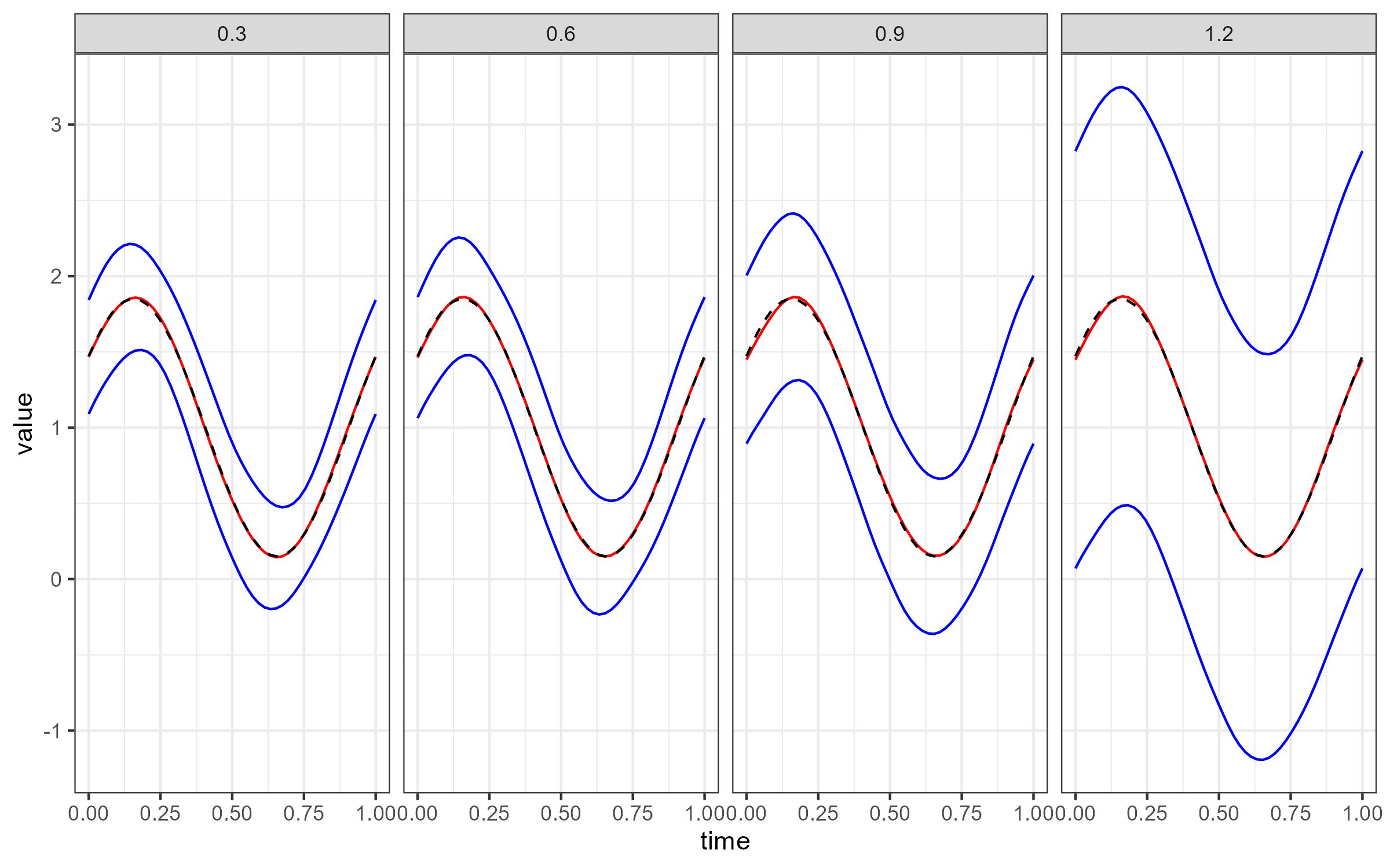
Figure 1: Confidence band of $\beta(t)$ on $20\times 20$ regular lattice with $\eta\in\{0.3,0.6,0.9,1.2\}$ in repeating lattice asymptotic context. The dotted black line is the true $\beta(t)$, the red line is the average of $\hat{\beta}(t)$, and the blue lines are the average of confidence bands of $\beta(t)$.

6 Concluding Remarks

We have developed a generalized linear model with a scalar response and a functional predictor that incorporates spatial dependence. Being able to account for such dependence improves the estimation of the regression parameter function, the usual focus of inference in regressions with functional covariates. The presence of the functional covariate process does not seem to degrade the estimation of the spatial structure in at least binary response variables. We have provided results that allow inference under the asymptotic context of a repeating lattice, and those results appear to be applicable under a fairly modest number of repetitions of the data situation ($20$ in our simulations). We can apply this model for practical applications with real-world data, such as analyzing the relationship between precipitation and flooding events, or between soil moisture levels and crop yields. However, having actual replications of a spatial problem may be less common than the alternative in which one must conduct an analysis using only one observed spatial field. We might conjecture that results similar to those presented here exist for the asymptotic context of an expanding lattice under strong mixing conditions on the spatial process, but any such results remain to be formally demonstrated.

Any number of potential extensions of this work are potentially of interest. Models that incorporate more complex spatial dependence such as directional or covariate-dependent spatial structure are a natural topic to consider. In this work, we used the AIC based truncation criterion of ¹⁶ for the selection of the number of basis functions to retain relative to the functional covariates. A number of other criteria for making this modeling decision are available, and the effect of the rule chosen on overall performance of estimation and inference procedures is an area for further investigation. Finally, we placed spatial dependence on the responses, conditional on the covariate process. It is possible one might encounter situations in which the functional covariate processes themselves exhibit spatial structure, either instead of or in addition to inherent spatial behavior in the response process, and this remains an area for future investigation.

*Conflict of interest

The authors declare no potential conflict of interests.

*Supporting information

Supplementary materials may be found in the online version of the article at the publisher’s website.

Proof of Theorems We use $C$ to denote a positive constant value that might vary in different inequalities.

Proof of Theorem 4.3

Proof .1.

According to Theorem 6.3.4 from ¹⁷, we will verify that for all $\epsilon>0$, there exists some large $\Delta>0$ depending on $\epsilon$ such that for all sufficiently large $N$,

$$P\left(\sup_{\tilde{\theta}:\|\tilde{\theta}-\theta\|_{2}\leq\Delta\sqrt{p_{N}\over N}{1\over b_{N}}}(\tilde{\theta}-\theta)^{\top}l_{c,N}^{\prime}(\tilde{\theta})\leq 0\right)\geq 1-\epsilon.$$

Note that, by Taylor expansion,

$$(\tilde{\theta}-\theta)^{\top}l_{c,N}^{\prime}(\tilde{\theta}) =(\tilde{\theta}-\theta)^{\top}l_{c,N}^{\prime}(\theta)+(\tilde{\theta}-\theta)^{\top}l_{c,N}^{\prime\prime}(\theta^{*})(\tilde{\theta}-\theta)\equiv A_{N1}+A_{N2}$$ (4)

for some $\theta^{*}$ with $\|\theta^{*}-\theta\|_{2}\leq\|\tilde{\theta}-\theta\|_{2}$. We have

$$E\|l_{c,N}^{\prime}(\theta)\|_{2}^{2} =E\left\|\sum_{k=1}^{N}l_{c}^{\prime}(\theta|\bm{y}_{k})\right\|_{2}^{2}=\sum_{k=1}^{N}E\left\|l_{c}^{\prime}(\theta|\bm{y}_{k})\right\|_{2}^{2}\leq CNp_{N}$$

by Assumption (A1), which implies $\|l_{c,N}^{\prime}(\theta)\|_{2}=O_{p}(\sqrt{Np_{N}}).$ Hence,

$$\sup_{\tilde{\theta}:\|\tilde{\theta}-\theta\|_{2}\leq\Delta\sqrt{p_{N}\over N}{1\over b_{N}}}|A_{N1}| \leq\sup_{\tilde{\theta}:\|\tilde{\theta}-\theta\|_{2}\leq\Delta\sqrt{p_{N}\over N}{1\over b_{N}}}\|\tilde{\theta}-\theta\|_{2}\|l_{c,N}^{\prime}(\theta)\|_{2}$$

$$=\Delta\sqrt{p_{N}\over N}{1\over b_{N}}O_{p}(\sqrt{Np_{N}})=\Delta O_{p}\left(p_{N}\over b_{N}\right).$$ (5)

Next, we write

$$A_{N2} =(\tilde{\theta}-\theta)^{\top}l_{c,N}^{\prime\prime}(\theta^{*})(\tilde{\theta}-\theta)$$

$$=(\tilde{\theta}-\theta)^{\top}(l_{c,N}^{\prime\prime}(\theta^{*})-l_{c,N}^{\prime\prime}(\theta))(\tilde{\theta}-\theta)$$

$$\quad+(\tilde{\theta}-\theta)^{\top}(l_{c,N}^{\prime\prime}(\theta)+NH(\theta))(\tilde{\theta}-\theta)$$

$$\quad-(\tilde{\theta}-\theta)^{\top}NH(\theta)(\tilde{\theta}-\theta)$$

$$\equiv A_{N21}+A_{N22}+A_{N23}.$$ (6)

From Lemma LABEL:lem1 and the assumption that $N^{-1/2}b_{N}^{-2}p_{N}\rightarrow 0$ as $N\rightarrow\infty$,

$$A_{N21} =(\tilde{\theta}-\theta)^{\top}(l_{c,N}^{\prime\prime}(\theta^{*})-l_{c,N}^{\prime\prime}(\theta))(\tilde{\theta}-\theta)$$

$$=\Delta^{2}O_{p}\left({p_{N}\over N}{1\over b_{N}^{2}}{\sqrt{N}p_{N}\over b_{N}}\right)=\Delta^{2}O_{p}\left({p_{N}^{2}\over\sqrt{N}}{1\over b_{N}^{3}}\right)=\Delta^{2}o_{p}\left(p_{N}\over b_{N}\right).$$ (7)

On the other hand, by Assumption (A3),

$$E\|{l_{c,N}^{\prime\prime}(\theta)+NH(\theta)}\|_{F}^{2} =E\left\|\sum_{k=1}^{N}\left(l_{c}^{\prime\prime}(\theta|\bm{y}_{k})-E[l_{c}^{\prime\prime}(\theta|\bm{y}_{k})]\right)\right\|_{F}^{2}$$

$$=\sum_{k=1}^{N}E\|l_{c}^{\prime\prime}(\theta|\bm{y}_{1})+H(\theta)\|_{F}^{2}$$

$$\leq{2N}\left\{E\|l_{c}^{\prime\prime}(\theta|\bm{y}_{1})\|_{F}^{2}+\|H(\theta)\|_{F}^{2}\right\}$$

$$\leq{4N}E\|l_{c}^{\prime\prime}(\theta|\bm{y}_{1})\|_{F}^{2}$$

$$\leq CNp_{N}^{2}$$

where the second last inequality is due to

$$\|H(\theta)\|_{F}^{2}=\|E(-l_{c}^{\prime\prime}(\theta|\bm{y}_{1}))\|_{F}^{2}\leq E\|l_{c}^{\prime\prime}(\theta|\bm{y}_{1})\|_{F}^{2}.$$

It implies $\|{l_{c,N}^{\prime\prime}(\theta)+NH(\theta)}\|_{F}=O_{p}(\sqrt{N}p_{N}).$ Then, we have

$$A_{N22} =(\tilde{\theta}-\theta)^{\top}(l_{c,N}^{\prime\prime}(\theta)+NH(\theta))(\tilde{\theta}-\theta)$$

$$=\Delta^{2}O_{p}\left({p_{N}\over N}{1\over b_{N}^{2}}\sqrt{N}p_{N}\right)=\Delta^{2}O_{p}\left({p_{N}^{2}\over\sqrt{N}}{1\over b_{N}^{2}}\right)=\Delta^{2}o_{p}\left(p_{N}\over b_{N}\right).$$ (8)

Also, we have

$$A_{N23} =-(\tilde{\theta}-\theta)^{\top}NH(\theta)(\tilde{\theta}-\theta)\leq-\Delta^{2}{p_{N}\over Nb_{N}^{2}}N\lambda_{min}(H(\theta))=-\Delta^{2}{p_{N}\over b_{N}}.$$ (9)

Thus, combining Equations (4)-(9),

$$\sup_{\tilde{\theta}:\|\tilde{\theta}-\theta\|_{2}\leq\Delta\sqrt{p_{N}\over N}{1\over b_{N}}}(\tilde{\theta}-\theta)^{\top}l_{c,N}^{\prime}(\tilde{\theta}) =\Delta R_{1N}+\Delta^{2}R_{2N}+\Delta^{2}R_{3N}-\Delta^{2}{p_{N}\over b_{N}},$$

with $R_{1N}=O_{p}(p_{N}/b_{N})$, $R_{2N}=o_{p}(p_{N}/b_{N})$, and $R_{3N}=o_{p}(p_{N}/b_{N})$. It implies that

$$P\left(\sup_{\tilde{\theta}:\|\tilde{\theta}-\theta\|_{2}\leq\Delta\sqrt{p_{N}\over N}{1\over b_{N}}}(\tilde{\theta}-\theta)^{\top}l_{c,N}^{\prime}(\tilde{\theta})\geq 0\right)$$

$$=P\left(\Delta R_{1N}+\Delta^{2}R_{2N}+\Delta^{2}R_{3N}\geq\Delta^{2}{p_{N}\over b_{N}}\right)$$

$$\leq P\left(\Delta R_{1N}\geq\Delta^{2}{p_{N}\over 3b_{N}}\right)+P\left(\Delta^{2}R_{2N}\geq\Delta^{2}{p_{N}\over 3b_{N}}\right)+P\left(\Delta^{2}|R_{3N}|\geq\Delta^{2}{p_{N}\over 3b_{N}}\right)$$

$$=P\left({R_{1N}\over p_{N}/b_{N}}\geq{\Delta\over 3}\right)+P\left({R_{2N}\over p_{N}/b_{N}}\geq{1\over 3}\right)+P\left({|R_{3N}|\over p_{N}/b_{N}}\geq{1\over 3}\right).$$

Since $R_{1N}=O_{p}(p_{N}/b_{N})$, $R_{2N}=o_{p}(p_{N}/b_{N})$, and $R_{3N}=o_{p}(p_{N}/b_{N})$, for all $\epsilon>0$, there exists $\Delta>0$ such that

$$\limsup_{N\rightarrow\infty}P\left(\sup_{\tilde{\theta}:\|\tilde{\theta}-\theta\|_{2}\leq\Delta\sqrt{p_{N}\over N}{1\over b_{N}}}(\tilde{\theta}-\theta)^{\top}l_{c,N}^{\prime}(\tilde{\theta})\geq 0\right)<\epsilon.$$

Equivalently, for all $\epsilon>0$, there exists $\Delta>0$ such that

$$\liminf_{N\rightarrow\infty}P\left(\sup_{\tilde{\theta}:\|\tilde{\theta}-\theta\|_{2}\leq\Delta\sqrt{p_{N}\over N}{1\over b_{N}}}(\tilde{\theta}-\theta)^{\top}l_{c,N}^{\prime}(\tilde{\theta})\leq 0\right)\geq 1-\epsilon.$$

Proof of Theorem 4.4

Proof .2.

We will use a similar argument as in ¹⁶. By Taylor expansion,

$$0=\bar{l}_{c,N}^{\prime}(\hat{\theta})=\bar{l}_{c,N}^{\prime}(\theta)+\bar{l}_{c,N}^{\prime\prime}(\theta^{*})^{\top}(\hat{\theta}-\theta)$$

for some $\theta^{*}$ with $\|\theta^{*}-\theta\|_{2}\leq\|\hat{\theta}-\theta\|_{2}$. Then,

$$\sqrt{N}(\hat{\theta}-\theta)$$

$$=-\left\{\bar{l}_{c,N}^{\prime\prime}(\theta^{*})\right\}^{-1}\sqrt{N}\bar{l}_{c,N}^{\prime}(\theta)$$

$$=\left\{{H(\theta)}+({\bar{l}_{c,N}^{\prime\prime}(\theta)-\bar{l}_{c,N}^{\prime\prime}(\theta^{*})})+({-\bar{l}_{c,N}^{\prime\prime}(\theta)-H(\theta)})\right\}^{-1}\sqrt{N}{\bar{l}_{c,N}^{\prime}(\theta)}$$

$$=\left\{I_{p_{N}+2}+H(\theta)^{-1}({\bar{l}_{c,N}^{\prime\prime}(\theta)-\bar{l}_{c,N}^{\prime\prime}(\theta^{*})})+H(\theta)^{-1}({-\bar{l}_{c,N}^{\prime\prime}(\theta)-H(\theta)})\right\}^{-1}\sqrt{N}H(\theta)^{-1}{\bar{l}_{c,N}^{\prime}(\theta)}$$

From Lemma LABEL:lem2,

$$\left\|\sqrt{N}(\hat{\theta}-\theta)-\sqrt{N}H(\theta)^{-1}\bar{l}_{c,N}^{\prime}(\theta)\right\|_{2}=o_{p}(1).$$

Recall that $W(\theta)=J(\theta)^{-1}=[w_{uv}]_{u,v=1}^{p_{n}+2}$. Note that, by Assumption (A4),

$$E\|G(\theta)\sqrt{N}H(\theta)^{-1}\bar{l}_{c,N}^{\prime}(\theta)\|_{2}^{2} =NE\|H(\theta)J(\theta)^{-1}\bar{l}_{c,N}^{\prime}(\theta)\|_{2}^{2}$$

$$=NE[\mathrm{tr}\{\bar{l}_{c,N}^{\prime}(\theta)^{\top}J(\theta)^{-1}H(\theta)H(\theta)J(\theta)^{-1}\bar{l}_{c,N}^{\prime}(\theta)\}]$$

$$=NE[\mathrm{tr}\{\bar{l}_{c,N}^{\prime}(\theta)\bar{l}_{c,N}^{\prime}(\theta)^{\top}J(\theta)^{-1}H(\theta)H(\theta)J(\theta)^{-1}\}]$$

$$=N^{-1}\mathrm{tr}\{J(\theta)J(\theta)^{-1}H(\theta)H(\theta)J(\theta)^{-1}\}$$

$$=N^{-1}\mathrm{tr}\{H(\theta)J(\theta)^{-1}H(\theta)\}=N^{-1}\mathrm{tr}\{G(\theta)\}$$

$$=O(N^{-1}).$$ (10)

and

$$\|G(\theta)\|_{F}^{2}=\mathrm{tr}\{G(\theta)^{2}\}\leq(\mathrm{tr}\{G(\theta)\})^{2}=O(1)$$ (11)

since $\mathrm{tr}(A^{2})\leq\{\mathrm{tr}(A)\}^{2}$ for symmetric positive semi-definite matrix $A$. Combining Equations (.2)-(11), we have

$$N(\hat{\theta}-\theta)^{\top}G(\theta)(\hat{\theta}-\theta)$$

$$=\left[\sqrt{N}H(\theta)^{-1}\bar{l}_{c,N}^{\prime}(\theta)+o_{p}(1)\right]^{\top}[H(\theta)J(\theta)^{-1}H(\theta)]\left[\sqrt{N}H(\theta)^{-1}\bar{l}_{c,N}^{\prime}(\theta)+o_{p}(1)\right]$$

$$=N{\bar{l}_{c,N}^{\prime}(\theta)}^{\top}H(\theta)^{-1}[H(\theta)J(\theta)^{-1}H(\theta)]H(\theta)^{-1}{\bar{l}_{c,N}^{\prime}(\theta)}+o_{p}(1)$$

$$=N^{-1}\left[\sum_{k=1}^{N}l_{c}^{\prime}(\theta|\bm{y}_{k})\right]^{\top}(J(\theta))^{-1}\left[\sum_{k=1}^{N}l_{c}^{\prime}(\theta|\bm{y}_{k})\right]+o_{p}(1)$$

$$=N^{-1}\sum_{u,v=1}^{p_{N}+2}\left\{\left[\sum_{k=1}^{N}{\partial l_{c}(\theta|\bm{y}_{k})\over\partial\theta}\right]_{u}w_{uv}\left[\sum_{k=1}^{N}{\partial l_{c}(\theta|\bm{y}_{k})\over\partial\theta}\right]_{v}\right\}+o_{p}(1)$$

$$\equiv A_{N}+B_{N}+o_{p}(1),$$ (12)

where

$$A_{N} =N^{-1}\sum_{k=1}^{N}\sum_{u,v=1}^{p_{N}+2}\left\{\left[{\partial l_{c}(\theta|\bm{y}_{k})\over\partial\theta}\right]_{u}w_{uv}\left[{\partial l_{c}(\theta|\bm{y}_{k})\over\partial\theta}\right]_{v}\right\}\quad\text{and}$$

$$B_{N} =N^{-1}\sum_{k\neq k^{\prime}}\sum_{u,v=1}^{p_{N}+2}\left\{\left[{\partial l_{c}(\theta|\bm{y}_{k})\over\partial\theta}\right]_{u}w_{uv}\left[{\partial l_{c}(\theta|\bm{y}_{k^{\prime}})\over\partial\theta}\right]_{v}\right\}.$$

From Lemma LABEL:lem3, it holds that

$${A_{N}-(p_{N}+2)\over\sqrt{p_{N}}}\xrightarrow[N\to\infty]{p}0.$$ (13)

Next, we will show that $B_{N}$ is asymptotically normal. Let

$$S_{Nj}=\sum_{k=1}^{j-1}\sum_{u,v=1}^{p_{N}+2}\left\{\left[{\partial l_{c}(\theta|\bm{y}_{k})\over\partial\theta}\right]_{u}w_{uv}\left[{\partial l_{c}(\theta|\bm{y}_{j})\over\partial\theta}\right]_{v}\right\}$$

so that

$$B_{N}={2\over N}\sum_{j=1}^{N}S_{Nj}.$$

From Lemma LABEL:lem4, the random variable $\{S_{Nj},1\leq j\leq N,N\in\mathbb{N}\}$ form a triangular array of the martingale difference sequences with respect to the filtrations $(\mathcal{F}_{Nj})=\sigma\left({\partial l_{c}(\theta|\bm{y}_{k})\over\partial\theta_{t}},1\leq k\leq j,1\leq t\leq p_{N}+2\right)$ ($1\leq j\leq N,N\in\mathbb{N}$). Let $\tilde{S}_{Nj}={2\over N\sqrt{2p_{N}}}S_{Nj}$. Then, it also forms a triangular array of the martingale difference sequences. From Lemma LABEL:lem5 and Lemma LABEL:lem6, we have

$$\sum_{j=1}^{N}E[\tilde{S}_{Nj}^{2}|\mathcal{F}_{N,j-1}]\xrightarrow[N\to\infty]{p}1$$

and

$$\sum_{j=1}^{N}E[\tilde{S}_{Nj}^{4}|\mathcal{F}_{N,j-1}]\xrightarrow[N\to\infty]{p}0.$$

Hence,

$${B_{N}\over\sqrt{2p_{N}}}\xrightarrow[N\rightarrow\infty]{d}N(0,1).$$ (14)

By Equations (.2)-(14), the asymptotic normality of quadratic form of $\hat{\theta}$ holds. Finally, the proof is completed by Lemma LABEL:lem7.

Proof of Theorem 4.5

Proof .3.

Note that, by Assumption (A4),

$$E\left\|(G_{22}^{(-1)}(\theta))^{-1}\sqrt{N}\begin{bmatrix}h_{21}^{(-1)}&h_{22}^{(-1)}\end{bmatrix}\bar{l}_{c,N}^{\prime}(\theta)\right\|_{2}^{2}$$

$$=NE\left\|(G_{22}^{(-1)}(\theta))^{-1}\begin{bmatrix}h_{21}^{(-1)}&h_{22}^{(-1)}\end{bmatrix}\bar{l}_{c,N}^{\prime}(\theta)\right\|_{2}^{2}$$

$$=NE\left[\mathrm{tr}\left\{\bar{l}_{c,N}^{\prime}(\theta)^{\top}\begin{bmatrix}h_{21}^{(-1)}&h_{22}^{(-1)}\end{bmatrix}^{\top}(G_{22}^{(-1)}(\theta))^{-2}\begin{bmatrix}h_{21}^{(-1)}&h_{22}^{(-1)}\end{bmatrix}\bar{l}_{c,N}^{\prime}(\theta)\right\}\right]$$

$$=N^{-1}\mathrm{tr}\left\{E[l_{c,N}^{\prime}(\theta)l_{c,N}^{\prime}(\theta)^{\top}]\begin{bmatrix}h_{21}^{(-1)}&h_{22}^{(-1)}\end{bmatrix}^{\top}(G_{22}^{(-1)}(\theta))^{-2}\begin{bmatrix}h_{21}^{(-1)}&h_{22}^{(-1)}\end{bmatrix}\right\}$$

$$=N^{-1}\mathrm{tr}\left\{\begin{bmatrix}h_{21}^{(-1)}&h_{22}^{(-1)}\end{bmatrix}\begin{bmatrix}j_{11}&j_{12}\\ j_{21}&j_{22}\end{bmatrix}\begin{bmatrix}h_{21}^{(-1)}&h_{22}^{(-1)}\end{bmatrix}^{\top}(G_{22}^{(-1)}(\theta))^{-2}\right\}$$

$$=N^{-1}\mathrm{tr}\left\{(h_{21}^{(-1)}j_{11}h_{12}^{(-1)}+h_{22}^{(-1)}j_{21}h_{12}^{(-1)}+h_{21}^{(-1)}j_{12}h_{22}^{(-1)}+h_{22}^{(-1)}j_{22}h_{22}^{(-1)})(G_{22}^{(-1)}(\theta))^{-2}\right\}$$

$$=N^{-1}\mathrm{tr}\left\{G_{22}^{(-1)}(\theta)(G_{22}^{(-1)}(\theta))^{-2}\right\}=N^{-1}\mathrm{tr}\left\{(G_{22}^{(-1)}(\theta))^{-1}\right\}$$

$$=N^{-1}\mathrm{tr}\left\{G_{22}(\theta)-G_{21}(\theta)G_{11}(\theta)^{-1}G_{12}(\theta)\right\}$$

$$\leq N^{-1}\mathrm{tr}\{G_{22}(\theta)\}$$

$$<N^{-1}\mathrm{tr}\{G(\theta)\}$$

$$=O(N^{-1}).$$ (15)

The fourth last equality is due to the definition of the block matrix and the third last inequality is because $G(\theta)$ is positive definite. From Lemma LABEL:lem2 and Equation (.3),

$$N(\hat{\beta}-\beta)^{\top}(G_{22}^{(-1)}(\theta))^{-1}(\hat{\beta}-\beta)$$

$$=N\bar{l}_{c,N}^{\prime}(\theta)^{\top}\begin{bmatrix}h_{12}^{(-1)}(G_{22}^{(-1)}(\theta))^{-1}h_{21}^{(-1)}&h_{12}^{(-1)}(G_{22}^{(-1)}(\theta))^{-1}h_{22}^{(-1)}\\ h_{22}^{(-1)}(G_{22}^{(-1)}(\theta))^{-1}h_{21}^{(-1)}&h_{22}^{(-1)}(G_{22}^{(-1)}(\theta))^{-1}h_{22}^{(-1)}\end{bmatrix}\bar{l}_{c,N}^{\prime}(\theta)+o_{p}(1)$$

$$={1\over N}\left[\sum_{k=1}^{N}l_{c}^{\prime}(\theta|\bm{y}_{k})\right]^{\top}\begin{bmatrix}h_{12}^{(-1)}(G_{22}^{(-1)}(\theta))^{-1}h_{21}^{(-1)}&h_{12}^{(-1)}(G_{22}^{(-1)}(\theta))^{-1}h_{22}^{(-1)}\\ h_{22}^{(-1)}(G_{22}^{(-1)}(\theta))^{-1}h_{21}^{(-1)}&h_{22}^{(-1)}(G_{22}^{(-1)}(\theta))^{-1}h_{22}^{(-1)}\end{bmatrix}\left[\sum_{k=1}^{N}l_{c}^{\prime}(\theta|\bm{y}_{k})\right]+o_{p}(1)$$

$$=A_{N,1}+B_{N,1}+o_{p}(1)$$ (16)

where

$$A_{N,1} ={1\over N}\sum_{k=1}^{N}\left\{l_{c}^{\prime}(\theta|\bm{y}_{k})^{\top}\begin{bmatrix}h_{12}^{(-1)}(G_{22}^{(-1)}(\theta))^{-1}h_{21}^{(-1)}&h_{12}^{(-1)}(G_{22}^{(-1)}(\theta))^{-1}h_{22}^{(-1)}\\ h_{22}^{(-1)}(G_{22}^{(-1)}(\theta))^{-1}h_{21}^{(-1)}&h_{22}^{(-1)}(G_{22}^{(-1)}(\theta))^{-1}h_{22}^{(-1)}\end{bmatrix}l_{c}^{\prime}(\theta|\bm{y}_{k})\right\}\quad\text{and}$$

$$B_{N,1} ={1\over N}\sum_{k\neq k^{\prime}}\left\{l_{c}^{\prime}(\theta|\bm{y}_{k})^{\top}\begin{bmatrix}h_{12}^{(-1)}(G_{22}^{(-1)}(\theta))^{-1}h_{21}^{(-1)}&h_{12}^{(-1)}(G_{22}^{(-1)}(\theta))^{-1}h_{22}^{(-1)}\\ h_{22}^{(-1)}(G_{22}^{(-1)}(\theta))^{-1}h_{21}^{(-1)}&h_{22}^{(-1)}(G_{22}^{(-1)}(\theta))^{-1}h_{22}^{(-1)}\end{bmatrix}l_{c}^{\prime}(\theta|\bm{y}_{k^{\prime}})\right\}.$$

From Lemma LABEL:lem8, it holds that

$${A_{N,1}-(p_{N}+1)\over\sqrt{p_{N}}}\xrightarrow[N\to\infty]{p}0.$$ (17)

Next, we will show that $B_{N,1}$ is asymptotically normal.
Recall that $Z(\theta)=\begin{bmatrix}h_{12}^{(-1)}(G_{22}^{(-1)}(\theta))^{-1}h_{21}^{(-1)}&h_{12}^{(-1)}(G_{22}^{(-1)}(\theta))^{-1}h_{22}^{(-1)}\\ h_{22}^{(-1)}(G_{22}^{(-1)}(\theta))^{-1}h_{21}^{(-1)}&h_{22}^{(-1)}(G_{22}^{(-1)}(\theta))^{-1}h_{22}^{(-1)}\end{bmatrix}$ and let

$$S_{Nj,1}=\sum_{k=1}^{j-1}\sum_{u,v=1}^{p_{N}+2}\left\{\left[{\partial l_{c}(\theta|\bm{y}_{k})\over\partial\theta}\right]_{u}z_{uv}\left[{\partial l_{c}(\theta|\bm{y}_{j})\over\partial\theta}\right]_{v}\right\}$$

so that

$$B_{N,1}={2\over N}\sum_{j=1}^{N}S_{Nj,1}.$$

By Lemma LABEL:lem9, the random variable $\{S_{Nj,1},1\leq j\leq N,N\in\mathbb{N}\}$ form a triangular array of the martingale difference sequences with respect to the filtrations $(\mathcal{F}_{Nj})=\sigma\left({\partial l_{c}(\theta|\bm{y}_{k})\over\partial\theta_{t}},1\leq k\leq j,1\leq t\leq p_{N}+2\right)$ ($1\leq j\leq N,N\in\mathbb{N}$). Let $\tilde{S}_{Nj,1}={2\over N\sqrt{2p_{N}}}S_{Nj,1}$. Then, it is also form a triangular array of the martingale difference sequences. From Lemma LABEL:lem10 and Lemma LABEL:lem11,

$$\sum_{j=1}^{N}E[\tilde{S}_{Nj,1}^{2}|\mathcal{F}_{N,j-1}]\xrightarrow[N\to\infty]{p}1$$

and

$$\sum_{j=1}^{N}E[\tilde{S}_{Nj,1}^{4}|\mathcal{F}_{N,j-1}]\xrightarrow[N\to\infty]{p}0.$$

Hence,

$${B_{N,1}\over\sqrt{2p_{N}}}\xrightarrow[N\rightarrow\infty]{d}N(0,1).$$ (18)

By Equations (.3)-(18), the asymptotic normality of quadratic form of $\hat{\beta}$ holds. Finally, the proof is completed by Lemma LABEL:lem12.

Proof of Theorem 4.6

Proof .4.

Recall that $e_{1}$ is a vector for which the first element is $1$ and the other elements are all $0$. From Lemma LABEL:lem2,

$$\sqrt{N}(G_{11}^{(-1)}(\theta))^{-1/2}(\hat{\eta}-\eta) =\sqrt{N}(G_{11}^{(-1)}(\theta))^{-1/2}e_{1}^{\top}H(\theta)^{-1}\bar{l}_{n}^{\prime}(\theta)+(G_{11}^{(-1)}(\theta))^{-1/2}o_{p}(1)$$

$$={1\over\sqrt{N}}(G_{11}^{(-1)}(\theta))^{-1/2}\sum_{k=1}^{N}e_{1}^{\top}H(\theta)^{-1}l_{c}^{\prime}(\theta|\bm{y}_{k})+o_{p}(1).$$

We have $(G_{11}^{(-1)}(\theta))^{-1}=O(1)$ because

$$G_{11}(\theta)G_{11}^{(-1)}(\theta) =1-G_{12}(\theta)G_{21}^{(-1)}(\theta)$$

$$=1+G_{12}(\theta)G_{22}^{(-1)}(\theta)G_{21}(\theta)G_{11}^{-1}(\theta)$$

$$>1$$

The first equality is due to $G(\theta)G^{-1}(\theta)=I_{p_{N}+2}$, the second equality is due to the definition of block matrix, and the last inequality is due to the assumption that $G(\theta)$ is positive definite. It implies $(G_{11}^{(-1)}(\theta))^{-1}<G_{11}(\theta)=O(1)$ by Assumption (A4). Let

$$S_{Nk,2}=e_{1}^{\top}H(\theta)^{-1}l_{c}^{\prime}(\theta|\bm{y}_{k}).$$

Note that the random variable $\{S_{Nk,2},1\leq k\leq N,N\in\mathbb{N}\}$ form a triangular array satisfying

$$ES_{Nk,2} =e_{1}^{\top}H(\theta)^{-1}El_{c}^{\prime}(\theta|\bm{y}_{k})=0,$$

$$ES_{Nk,2}^{2} =E[e_{1}^{\top}H(\theta)^{-1}l_{c}^{\prime}(\theta|\bm{y}_{1})l_{c}^{\prime}(\theta|\bm{y}_{1})^{\top}H(\theta)^{-1}e_{1}]=G_{11}^{(-1)}(\theta),$$

$$E\left[\sum_{k=1}^{N}S_{Nk,2}^{2}\right] =\sum_{k=1}^{N}ES_{Nk,2}^{2}=NG_{11}^{(-1)}(\theta).$$

By Assumption (E1), we have

$$(NG_{11}^{(-1)}(\theta))^{-2}\sum_{k=1}^{N}E[S_{Nk,2}^{4}]$$

$$=(NG_{11}^{(-1)}(\theta))^{-2}\sum_{k=1}^{N}E[(e_{1}^{\top}H(\theta)^{-1}l_{c}^{\prime}(\theta|\bm{y}_{k}))^{4}]=o(1),$$

which implies, by the Lyapunov CLT,

$$(NG_{11}^{(-1)}(\theta))^{-1/2}\sum_{k=1}^{N}S_{Nk,2}\xrightarrow{\text{d}}{N}N(0,1).$$

That is,

$$\sqrt{N}(G_{11}^{(-1)}(\theta))^{-1/2}(\hat{\eta}-\eta)\xrightarrow{\text{d}}{N}N(0,1).$$

Finally, the proof is completed by Lemma LABEL:lem13.

References

- Besag 1974 Besag, Julian 1974. “Spatial interaction and the statistical analysis of lattice systems.” Journal of the Royal Statistical Society: Series B (Methodological) 36(2): 192–225.
- Cardot et al. 1999 Cardot, Hervé, Frédéric Ferraty, and Pascal Sarda. 1999. “Functional linear model.” Statistics & Probability Letters 45(1): 11–22.
- Cardot and Sarda 2005 Cardot, Hervé, and Pacal Sarda. 2005. “Estimation in generalized linear models for functional data via penalized likelihood.” Journal of Multivariate Analysis 92(1): 24–41.
- Goldsmith et al. 2011 Goldsmith, Jeff, Jennifer Bobb, Ciprian M Crainiceanu, Brian Caffo, and Daniel Reich. 2011. “Penalized functional regression.” Journal of computational and graphical statistics 20(4): 830–851.
- Hall and Horowitz 2007 Hall, Peter, and Joel L Horowitz. 2007. “Methodology and convergence rates for functional linear regression.” The Annals of Statistics 35(1): 70–91.
- Horváth and Kokoszka 2012 Horváth, Lajos, and Piotr Kokoszka. 2012. Inference for functional data with applications, , Vol 200. Springer Science & Business Media.
- Hsing and Eubank 2015 Hsing, Tailen, and Randall Eubank. 2015. Theoretical foundations of functional data analysis, with an introduction to linear operators, , Vol 997. John Wiley & Sons.
- Jadhav et al. 2017 Jadhav, S, HL Koul, and Q Lu. 2017. “Dependent generalized functional linear models.” Biometrika 104(4): 987–994.
- James 2002 James, Gareth M 2002. “Generalized linear models with functional predictors.” Journal of the Royal Statistical Society: Series B (Statistical Methodology) 64(3): 411–432.
- James and Silverman 2005 James, Gareth M, and Bernard W Silverman. 2005. “Functional adaptive model estimation.” Journal of the American Statistical Association 100(470): 565–576.
- Kaiser et al. 2012 Kaiser, Mark S, Petruţa C Caragea, and Kyoji Furukawa. 2012. “Centered parameterizations and dependence limitations in Markov random field models.” Journal of Statistical Planning and Inference 142(7): 1855–1863.
- Kaiser and Cressie 2000 Kaiser, Mark S, and Noel Cressie. 2000. “The construction of multivariate distributions from Markov random fields.” Journal of Multivariate Analysis 73(2): 199–220.
- Kokoszka and Reimherr 2017 Kokoszka, Piotr, and Matthew Reimherr. 2017. Introduction to Functional Data Analysis, Chapman and Hall/CRC.
- Manuel and Scalon 2020 Manuel, Lourenço, and João D Scalon. 2020. “Generalized estimating equations approach for spatial lattice data: A case study in adoption of improved maize varieties in Mozambique.” Biometrical Journal 62(8): 1879–1895.
- Martínez-Hernández and Genton 2020 Martínez-Hernández, Israel, and Marc G Genton. 2020. “Recent developments in complex and spatially correlated functional data.” Brazilian Journal of Probability and Statistics 34(2): 204–229.
- Müller and Stadtmüller 2005 Müller, Hans-Georg, and Ulrich Stadtmüller. 2005. “Generalized functional linear models.” the Annals of Statistics 33(2): 774–805.
- Ortega and Rheinboldt 2000 Ortega, James M, and Werner C Rheinboldt. 2000. Iterative solution of nonlinear equations in several variables, SIAM.
- Ramsay and Silverman 2005 Ramsay, James O, and Bernhard W Silverman. 2005. Functional Data Analysis, Springer-Verlag New York.
- Varin et al. 2011 Varin, Cristiano, Nancy Reid, and David Firth. 2011. “An overview of composite likelihood methods.” . Statistica Sinica: 5–42.
- Wang 2011 Wang, Lan 2011. “GEE analysis of clustered binary data with diverging number of covariates.” The Annals of Statistics 39(1): 389–417.
- Yao et al. 2005 Yao, Fang, Hans-Georg Müller, and Jane-Ling Wang. 2005. “Functional linear regression analysis for longitudinal data.” The Annals of Statistics 33(6): 2873–2903.