Investigating the Histogram Loss in Regression

Abstract

It is becoming increasingly common in regression to train neural networks that model the entire distribution even if only the mean is required for prediction. This additional modeling often comes with performance gain and the reasons behind the improvement are not fully known. This paper investigates a recent approach to regression, the Histogram Loss, which involves learning the conditional distribution of the target variable by minimizing the cross-entropy between a target distribution and a flexible histogram prediction. We design theoretical and empirical analyses to determine why and when this performance gain appears, and how different components of the loss contribute to it. Our results suggest that the benefits of learning distributions in this setup come from improvements in optimization rather than learning a better representation. We then demonstrate the viability of the Histogram Loss in common deep learning applications without a need for costly hyperparameter tuning.

Keywords: Neural Networks, Regression, Conditional Density Estimation

1 Introduction

A fundamental problem in machine learning is regression which considers predicting a real-valued output variable from a set of input variables with the goal of making predictions as close as possible to the true values. In regression, a common loss function is the squared-error loss, or $\ell_{2}$ loss. This corresponds to assuming that the continuous target variable $Y$ is Gaussian distributed, conditioned on inputs $\mathbf{x}\in\mathbb{R}^{d}$: $Y\sim\mathcal{N}(\mu=f(\mathbf{x}),\sigma^{2})$ for a fixed variance $\sigma^{2}>0$ and some function $f:\mathbb{R}^{d}\rightarrow\mathbb{R}$ on the inputs from a function class $\mathcal{F}$, such as a linear function $f(\mathbf{x})=\langle\mathbf{x},\mathbf{w}\rangle$ for weights $\mathbf{w}\in\mathbb{R}^{d}$. The maximum likelihood function $f$ for $n$ samples $((\mathbf{x}_{j},y_{j}))_{j=1}^{n}$, corresponds to minimizing the $\ell_{2}$ loss

$$\min_{f\in\mathcal{F}}\sum_{j=1}^{n}(f(\mathbf{x}_{j})-y_{j})^{2}$$ (1)

with prediction $f(\mathbf{x})\approx\mathbb{E}[Y|\mathbf{x}]$ (Bishop, 2006).

The squared-error loss is not the only choice for regression. Properties like ease of optimization, improved generalization, and robustness to outliers motivate designing alternative loss functions. Loss functions such as $\ell_{1}$ loss, Huber loss, and Charbonnier loss have shown improvements in presence of outliers (Huber, 2011; Charbonnier et al., 1994; Barron, 2019).

A more radical alternative is to reparameterize the model to capture a fuller picture of the output distribution. Examples are predicting the means, variances, and coefficients of a multi-modal mixture of Gaussian distributions (Bishop, 1994), weights of a histogram (Rothe et al., 2015), quantiles of a distribution (Dabney et al., 2018b), and a generative model for sampling from the distribution (Dabney et al., 2018a). In deep learning literature such reparameterizations have been beneficial in applications such as age estimation, depth estimation, and value prediction for decision making (Gao et al., 2017; Reading et al., 2021; Bellemare et al., 2017; Hessel et al., 2018; Bellemare et al., 2023). Understanding why these approaches can be superior to the squared loss, even when only the mean of the predicted distribution is needed, is an ongoing endeavour, and a common explanation is that the extra difficulty helps the network learn a better representation (Bellemare et al., 2017; Lyle et al., 2019, 2021; Lan et al., 2022).

Figure 1: Training with HL. The red curve is the target distribution and the blue histogram is the prediction distribution. The neural network is trained to minimize the cross-entropy between the two.

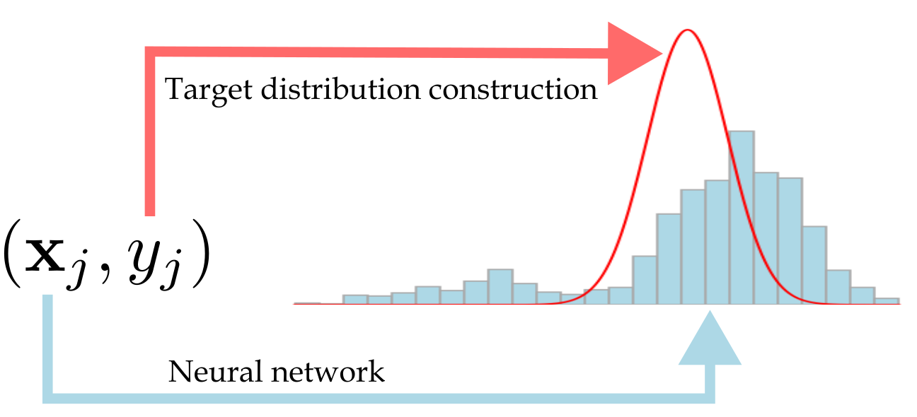
A shorter version of this paper by Imani and White (2018) proposed a family of loss functions called the Histogram Loss (HL). In short, a model trained with HL outputs the prediction distribution, a histogram parameterized by a softmax function. Each scalar target in the training data is converted to a target distribution and the model aims to match the histogram to the target distribution by reducing the cross-entropy between the two. The process is shown in Figure 1. Imani and White (2018) showed the feasibility of HL on four regression datasets and provided a bound on the norm of the loss as well as a small-scale empirical study towards understanding why HL can outperform the squared error loss.

Our goal in this paper is to expand the theoretical understanding of this loss, delve deeper into the reasons behind the benefits of HL, and explore the viability of HL in larger-scale deep learning tasks and provide rules of thumb for its hyperparameters. We will also include the results by Imani and White (2018) for completeness. The following list summarizes the novel contributions.

1. A theoretical analysis of HL is provided. First, the bias of the loss is characterized and bounded under a minor simplification regarding the support of the prediction distribution. Second, we show that minimizing HL reduces an upper bound on the difference between the predictions and the targets in the training data.

2. We conduct a larger empirical study compared to Imani and White (2018) to test hypotheses regarding the performance of HL. On four regression datasets, we test

   1. if the choice of target distribution has a major impact on the bias of HL that can explain the difference in error rates,

   2. if properties of the histogram prediction and target distribution give rise to a bias-variance trade-off,

   3. if the challenge in the task of predicting a full distribution forces the model to learn a better representation,

   4. if switching from the $\ell_{2}$ loss to HL helps gradient descent’s search for a good solution by making the landscape smoother,

   5. if HL is more robust to corrupted targets in the dataset, and

   6. if HL finds a model whose output is less sensitive to input perturbations.

3. We show viability of HL on large-scale time series and value prediction tasks with different architectures and provide heuristics for choosing the hyperparameters of the loss, namely the number of bins and the amount of padding in the histogram and the degree of smoothing in the target distribution. A fixed set of recommended hyperparameter values works well in a diverse set of experiments.

This paper consists of 6 sections. In Section 2 we introduce the Histogram Loss along with a discussion on constructing the target distribution. Sections 3 and 4 provide extensive theoretical and empirical analyses of the proposed method. Section 5 shows results on time series and value prediction using different architectures. Finally, Section 6 concludes the paper.

2 Distributional Losses for Regression

In this section we introduce the Histogram Loss (HL). We first introduce the loss and describe how it can be used for regression. Then we discuss the design choices in constructing the target function and relate them to other objectives, including maximum likelihood for regression and other methods that learn distributions.

2.1 The Histogram Loss

As Figure 1 illustrated, training and inference with HL involves estimating the conditional distribution of the target. For training, the scalar target in the regression dataset has to be converted to a target distribution. The method for converting a scalar target to a target distribution is a design choice that we will describe later in this section. The corresponding input in the dataset is fed to the network which outputs what we call the prediction distribution. HL is the cross-entropy between the target distribution and the prediction distribution. For inference, a new input is fed to the network and the mean of the prediction distribution is used as the final prediction.

More formally, consider predicting a continuous target $Y$ with event space $\mathcal{Y}$, given inputs $\mathbf{x}$. Recall that directly predicting $Y$ is possible by minimizing the squared error on samples $(\mathbf{x}_{j},y_{j})$ where input $\mathbf{x}_{j}\in\mathbb{R}^{d}$ is associated with target $y_{j}\in\mathbb{R}$. Instead of directly predicting $Y$, we can learn a distribution on $Y|\mathbf{x}$ whose expected value will be used as the prediction. Assume we have samples $(\mathbf{x}_{j},q_{j})$, where each input $\mathbf{x}_{j}$ is associated with a target distribution with pdf $q_{j}:\mathcal{Y}\rightarrow[0,1]$. We would like to learn a parameterized prediction distribution $h_{\mathbf{x}}:\mathcal{Y}\rightarrow[0,1]$, conditioned on $\mathbf{x}$, by minimizing a measure of difference between $h_{\mathbf{x}}$ and $q$.

Figure 2: (Top) A sample histogram, and (bottom) a neural network with a softmax output layer that represents a histogram.

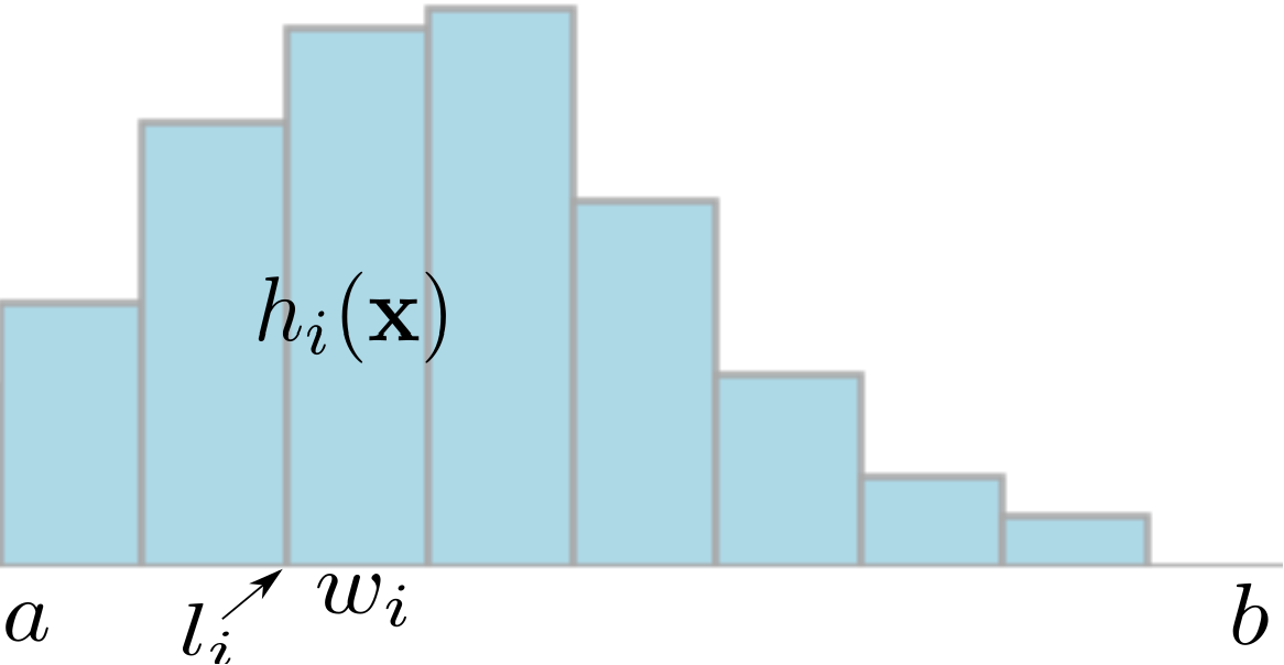
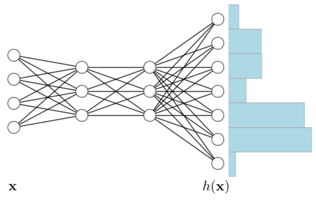
Three choices have to be made to learn a distribution on $Y|\mathbf{x}$ in this setting. First, we need a parameterization for $h_{\mathbf{x}}$ which is a continuous probability density function. Second, we require a function that measures how the prediction distribution is different from the target distribution. Third, we need a method to convert a regression dataset with samples $(\mathbf{x}_{j},y_{j})$ with real-valued outputs to one with samples $(\mathbf{x}_{j},q_{j})$ whose outputs are target distributions. Below we detail the first two choices and in the next section we describe several methods for constructing target distributions.

We propose to restrict the prediction distribution $h_{\mathbf{x}}$ to be a histogram density. Assume an interval $[a,b]$ on the real line has been uniformly partitioned into $k$ bins, of width $w_{i}$, and let function $h:\mathcal{X}\rightarrow[0,1]^{k}$ provide $k$-dimensional vector $h(\mathbf{x})$ of the coefficients indicating the probability the target is in that bin, given $\mathbf{x}$. The density $h_{\mathbf{x}}$ corresponds to a (normalized) histogram, and has density values $h_{i}(\mathbf{x})/w_{i}$ per bin. A sample histogram is depicted in Figure 2 (top). The histogram prediction distribution $h_{\mathbf{x}}$ can be parameterized with a softmax output layer in a neural network. The softmax layer has $k$ units and the value of unit $i$ represents $h_{i}(\mathbf{x})$. Figure 2 (bottom) shows a sample neural network whose output represents a histogram.

For the measure of difference, we use the KL-divergence. Suppose the target distribution has CDF $F$ and the support of this distribution is within the range $[a,b]$. The KL-divergence between $q$ and $h_{\mathbf{x}}$ is

$$D_{KL}(q||h_{\mathbf{x}}) =-\int_{a}^{b}q(y)\log\frac{h_{\mathbf{x}}(y)}{q(y)}dy$$

$$=-\int_{a}^{b}q(y)\log h_{\mathbf{x}}(y)dy-\biggl{(}-\int_{a}^{b}q(y)\log q(y)dy\biggr{)}$$

Because the second term only depends on $q$, the aim is to minimize the first term: the cross-entropy between $q$ and $h_{\mathbf{x}}$. This loss simplifies, due to the histogram form on $h_{\mathbf{x}}$:

$$-\int_{a}^{b}q(y)\log h_{\mathbf{x}}(y)dy =-\sum_{i=1}^{k}\int_{l_{i}}^{l_{i}+w_{i}}q(y)\log\frac{h_{i}(\mathbf{x})}{w_{i}}dy$$

$$=-\sum_{i=1}^{k}\log\frac{h_{i}(\mathbf{x})}{w_{i}}\underbrace{(F(l_{i}+w_{i})-F(l_{i}))}_{c_{i}}.$$

In the minimization, the width itself can be ignored, because $\log\tfrac{h_{i}(\mathbf{x})}{w_{i}}=\log h_{i}(\mathbf{x})-\log w_{i}$, giving the Histogram Loss

$$HL(q,h_{\mathbf{x}})=-\sum_{i=1}^{k}c_{i}\log h_{i}(\mathbf{x}).$$ (2)

This loss has several useful properties. One important property is that it is convex in $h_{i}(\mathbf{x})$; even if the loss is not convex in all network parameters, it is at least convex on the last layer. The other two benefits are due to restricting the form of the predicted distribution $h_{\mathbf{x}}$ to be a histogram density. First, the divergence to the full distribution $q$ can be efficiently computed. Second, the choice of $q$ is flexible, as long as its CDF can be evaluated for each bin. The weighting $c_{i}=F(l_{i}+w_{i})-F(l_{i})$ can be computed offline once for each sample, making it inexpensive to query repeatedly for each sample during training.

2.2 Target Distributions

The Histogram Loss requires a target distribution corresponding to each input. The method for constructing a target distribution from the target $y_{j}$ in the dataset can be chosen upfront. Different choices simply result in different weightings in HL. Below, we consider some special cases that are of interest.

Truncated Gaussian on $Y|\mathbf{x}$ (HL-Gaussian).    Consider a truncated Gaussian distribution, on support $[a,b]$, as the target distribution. The mean $\mu$ for this Gaussian is the datapoint $y_{j}$ itself, with fixed variance $\sigma^{2}$. The pdf $q$ is

$$q(y)=\frac{1}{Z\sigma\sqrt{2\pi}}e^{-\frac{(y-\mu)^{2}}{2\sigma^{2}}}$$

where $Z=\frac{1}{2}(\text{erf}\left(\frac{b-\mu}{\sqrt{2}\sigma}\right)-\text{erf}\left(\frac{a-\mu}{\sqrt{2}\sigma}\right))$, and HL has

$$c_{i}=\tfrac{1}{2Z}\left(\text{erf}\left(\frac{l_{i}+w_{i}-\mu}{\sqrt{2}\sigma}\right)-\text{erf}\left(\frac{l_{i}-\mu}{\sqrt{2}\sigma}\right)\right).$$

This distribution enables smoothing over $Y$, through the variance parameter $\sigma^{2}$. We call this loss HL-Gaussian, defined by number of bins $k$ and variance $\sigma^{2}$. Based on positive empirical performance, it will be the main HL loss that we advocate for and analyze.

Dirac delta on $Y|\mathbf{x}$ (HL-OneBin).    Consider Gaussians centered around datapoints $y_{j}$, with arbitrarily small variances $\tfrac{1}{2}a^{2}$:

$$\delta_{a,j}(y)=\frac{1}{a^{2}\sqrt{\pi}}\exp\left(-\tfrac{(y-y_{j})^{2}}{a^{2}}\right).$$

Let the target distribution have $q(y)=\delta_{a,j}(y)$ for each sample. Define function $c_{i,j}:[0,\infty)\rightarrow[0,1]$ as $c_{i,j}(a)=\int_{l_{i}}^{l_{i}+w_{i}}\delta_{a,j}(y)dy$ . For each $y_{j}$, as $a\rightarrow 0$, $c_{i,j}(a)\rightarrow 1$ if $y_{j}\in[l_{i},l_{i}+w_{i}]$ and $c_{i,j}(a)\rightarrow 0$ otherwise. So, for $i_{j}$ s.t. $y_{j}\!\in[l_{i_{j}},l_{i_{j}}\!+\!w_{i}]$,

$$\!\!\lim_{a\rightarrow 0}\!HL(\delta_{a,j},h_{\mathbf{x}_{j}}) =-\log h_{i_{j}}(\mathbf{x}_{j}).$$

The sum over samples for HL to the Dirac delta on $Y|\mathbf{x}$, then, corresponds to the negative log-likelihood for $h_{\mathbf{x}}$

$$\mathop{\mathrm{argmin}}_{h_{1},\ldots,h_{k}}-\sum_{j=1}^{n}\log h_{i_{j}}(\mathbf{x}_{j}) =\mathop{\mathrm{argmin}}_{h_{1},\ldots,h_{k}}-\sum_{j=1}^{n}\log h_{\mathbf{x}_{j}}(y_{j}).$$

Such a delta distribution on $Y|\mathbf{x}$ results in one coefficient $c_{i}$ being 1, reflecting the distributional assumption that $Y$ is certainly in a bin. In the experiments, we compare to this loss, which we call HL-OneBin.

Mixture of Dirac delta and uniform on $Y|\mathbf{x}$ (HL-Uniform).    Using a similar analysis to above, $q(y)$ can be considered as a mixture between $\delta_{a,j}(y)$ and a uniform distribution. For a weighting of $\epsilon$ on the uniform distribution, the resulting loss HL-Uniform has $c_{i}=\epsilon$ for $i\neq i_{j}$, and $c_{i_{j}}=1-(k-1)\epsilon$.

3 Theoretical Analysis

This section assembles our theoretical results on the Histogram Loss. The first part considers the behavior of gradient descent optimization on HL and the $\ell_{2}$ loss. Gradient descent is a local search method, and problems like the existence of highly varying regions, unfavorable local minima and saddle points, and poorly conditioned coordinates can hinder the search. A complete characterization of the loss surface is a hard problem. Instead, we provide an upper bound on the norm of the gradient of HL which suggests that the gradient varies less through the training and provides more reliable optimization steps. We also point out how this norm relates to the generalization performance of the model. The second part shows a similarity between minimizing HL and entropy-regularized policy improvement based on recent work by Norouzi et al. (2016). The third part discusses the bias of the minimizer of HL. The mean of the target generating distribution can be different from a coarse histogram prediction distribution that approximates it. We show that, when KL-divergence to data points with Gaussian target distributions is minimized, this difference is bounded by half of the bin width as long as the target distribution has negligible probability beyond the support of the histogram. The last part shows that minimizing HL on the data reduces an upper bound on the difference between the targets and the mean of prediction distributions.

3.1 Stable gradients for the Histogram Loss

Hardt et al. (2016) have shown that the generalization performance for stochastic gradient descent is bounded by the number of steps that stochastic gradient descent takes during training, even for non-convex losses. The bound is also dependent on the properties of the loss. In particular, it is beneficial to have a loss function with small Lipschitz constant $L$, which bounds the norm of the gradient. Below, we discuss how HL with a Gaussian distribution (HL-Gaussian) in fact promotes an improved bound on this norm, over both the $\ell_{2}$ loss and HL with all weight in one bin (HL-OneBin).

In the proposition bounding HL-Gaussian gradient, we assume

$$h_{i}(\mathbf{x})=\tfrac{\exp(\boldsymbol{\phi}_{\boldsymbol{\theta}}(\mathbf{x})^{\top}\mathbf{w}_{i})}{\sum_{j=1}^{k}\exp(\boldsymbol{\phi}_{\boldsymbol{\theta}}(\mathbf{x})^{\top}\mathbf{w}_{j})}$$ (3)

for some function $\boldsymbol{\phi}_{\boldsymbol{\theta}}:\mathcal{X}\rightarrow\mathcal{R}^{k}$ parameterized by a vector of parameters ${\boldsymbol{\theta}}$. For example, $\boldsymbol{\phi}_{\boldsymbol{\theta}}(\mathbf{x})$ could be the last hidden layer in a neural network, with parameters ${\boldsymbol{\theta}}$ for the entire network up to that layer. The proposition provides a bound on the gradient norm in terms of the current network parameters. Our goal is to understand how the gradients might vary locally for the parameters, as opposed to globally bounding the norm and characterizing the Lipschitz constant only in terms of the properties of the function class and loss.

Proposition 1 (Local Lipschitz constant for HL-Gaussian)

Assume $\mathbf{x},y$ are fixed, giving fixed coefficients $c_{i}$ in HL-Gaussian. Let $h_{i}(\mathbf{x})$ be as in (3), defined by the parameters $\mathbf{w}=\{\mathbf{w}_{1},\ldots,\mathbf{w}_{k}\}$ and ${\boldsymbol{\theta}}$, providing the predicted distribution $h_{\mathbf{x}}$. Assume for all $i$ that $\mathbf{w}_{i}^{\top}\boldsymbol{\phi}_{\boldsymbol{\theta}}(\mathbf{x})$ is locally $l$-Lipschitz continuous w.r.t. ${\boldsymbol{\theta}}$

$$\|\nabla_{\boldsymbol{\theta}}(\mathbf{w}_{i}^{\top}\boldsymbol{\phi}_{\boldsymbol{\theta}}(\mathbf{x}))\|\leq l$$ (4)

Then the norm of the gradient for HL-Gaussian, w.r.t. all the parameters in the network $\{{\boldsymbol{\theta}},\mathbf{w}\}$, is bounded by

$$\|\nabla_{{\boldsymbol{\theta}},\mathbf{w}}HL(q,h_{\mathbf{x}})\|\leq\left(l+\|\boldsymbol{\phi}_{\boldsymbol{\theta}}(\mathbf{x})\|\right)\sum_{i=1}^{k}|c_{i}-h_{i}(\mathbf{x})|$$ (5)

The results by Hardt et al. (2016) suggest it is beneficial for the local Lipschitz constant—or the norm of the gradient—to be small on each step. HL-Gaussian provides exactly this property. Besides the network architecture—which we are here assuming is chosen outside of our control—HL-Gaussian gradient norm is proportional to $|c_{i}-h_{i}(\mathbf{x})|$. This number is guaranteed to be less than 1, but generally is likely to be even smaller, especially if $h_{i}(\mathbf{x})$ reasonably accurately predicts $c_{i}$. Further, the gradients should push the weights to stay within a range specified by $c_{i}$, rather than preferring to push some to be very small—close to 0—and others to be close to 1. For example, if $h_{i}(\mathbf{x})$ starts relatively uniform, then the objective does not encourage predictions $h_{i}(\mathbf{x})$ to get smaller than $c_{i}$. If $c_{i}$ are non-negligible, this keeps $h_{i}(\mathbf{x})$ away from zero and the loss in a smaller range.

This contrasts both the norm of the gradient for the $\ell_{2}$ loss and HL-OneBin. For the $\ell_{2}$ loss, $(f(\mathbf{x})-y)\Bigl{[}\negthinspace\begin{smallmatrix}\nabla_{\boldsymbol{\theta}}\mathbf{w}^{\top}\boldsymbol{\phi}_{\boldsymbol{\theta}}(\mathbf{x})\\ \boldsymbol{\phi}_{\boldsymbol{\theta}}(\mathbf{x})\end{smallmatrix}\Bigr{]}$ is the gradient, giving gradient norm bound $(l+\|\boldsymbol{\phi}_{\boldsymbol{\theta}}(\mathbf{x})\|)|f(\mathbf{x})-y|$. The constant $|f(\mathbf{x})-y|$, as opposed to $\sum_{i=1}^{k}|c_{i}-h_{i}(\mathbf{x})|$, can be much larger, even if $y$ is normalized between $[0,1]$, and can vary considerably more. HL-OneBin, on the other hand, shares the same constant as HL-Gaussian, but suffers from another problem. The Lipschitz constant $l$ in Equation (4) will likely be larger, because $c_{i}$ is frequently zero and so pushes $h_{i}(\mathbf{x})$ towards zero. This results in larger objective values and pushes $\mathbf{w}_{i}^{\top}\boldsymbol{\phi}_{\boldsymbol{\theta}}(\mathbf{x})$ to get larger, to enable $h_{i}(\mathbf{x})$ to get close to 1.

3.2 Connection to Reinforcement Learning

HL can also be motivated through a connection to maximum entropy reinforcement learning. In Reinforcement Learning, an agent iteratively selects actions and transitions between states to maximize (long-term) reward. The agent’s goal is to find an optimal policy, in as few interactions as possible. To do so, the agent begins by exploring more, to then enable more efficient convergence to optimal. Supervised learning can be expressed as a reinforcement learning problem (Norouzi et al., 2016), where action selection conditioned on a state corresponds to making a prediction conditioned on a feature vector. An alternative view to minimizing prediction error is to search for a policy to make accurate predictions.

One strategy to efficiently find an optimal policy is through a maximum entropy objective. The policy balances between selecting the action it believes to be optimal—make its current best prediction—and acting more randomly—with high-entropy. For continuous action set $\mathcal{Y}$, the goal is to minimize the following objective

$$\int_{\mathcal{X}}p_{s}(\mathbf{x})\Big{[}-\tau H(h_{\mathbf{x}})-\int_{\mathcal{Y}}h_{\mathbf{x}}(y)r(y,y_{i})dy\Big{]}d\mathbf{x}$$ (6)

where $\tau>0$; $p_{s}$ is a distribution over states $\mathbf{x}$; $h_{\mathbf{x}}$ is the policy or distribution over actions for a given $\mathbf{x}$; $H(\cdot)$ is the differential entropy—the extension of entropy to continuous random variables; and $r(y,y_{i})$ is the reward function, such as the negative of the objective $r(y,y_{i})=-\tfrac{1}{2}(y-y_{i})^{2}$. Minimizing (6) corresponds to minimizing the KL-divergence across $\mathbf{x}$ between $h_{\mathbf{x}}$ and the exponentiated payoff distribution $q(y)=\frac{1}{Z}\exp(r(y,y_{i})/\tau)$ where $Z=\int\exp(r(y,y_{i})/\tau)$, because

$$D_{KL}(h_{\mathbf{x}}||q) =-H(h_{\mathbf{x}})-\int h_{\mathbf{x}}(y)\log q(y)dy$$

$$=-H(h_{\mathbf{x}})-\tau^{-1}\int h_{\mathbf{x}}(y)r(y,y_{i})dy+\log Z.$$

The connection between HL and maximum-entropy reinforcement learning is that both are minimizing a divergence to this exponentiated distribution $p$. HL, however, is minimizing $D_{KL}(q||h_{\mathbf{x}})$ instead of $D_{KL}(h_{\mathbf{x}}||q)$. For example, Gaussian target distribution with variance $\sigma^{2}$ corresponds to minimizing $D_{KL}(q||h_{\mathbf{x}})$ with $r(y,y_{i})=-\tfrac{1}{2}(y-y_{i})^{2}$ and $\tau=\sigma^{2}$. These two KL-divergences are not the same, but a similar argument to Norouzi et al. (2016) could be extended for continuous $y$, showing $D_{KL}(h_{\mathbf{x}}||q)$ is upper-bounded by $D_{KL}(q||h_{\mathbf{x}})$ plus variance terms. The intuition, then, is that minimizing HL is promoting an efficient search for an optimal (prediction) policy.

3.3 Bias of the Histogram Loss

Different forms of bias can be induced by components of the Histogram Loss, namely using histogram densities, using the KL-divergence, and due to the chosen type of target distribution. This section explores the effects of these components on the bias. First we characterize the minimizer of HL and the effect of target distribution on it. Then we show to what extent the mean of the minimizer differs from the target generating distribution.

We make two assumptions in this section to simplify the analysis and highlight the key points. First, we assume that the model is flexible enough so that the predicted distribution for each input can be optimized independently. Therefore we consider the case where all the data points in the dataset have the same input and drop the subscripts that show dependence on $\mathbf{x}$. Second, we assume that the bins have equal width $w$ and the support of the histogram is unbounded and therefore the target distribution is not truncated. This assumption is approximately met in the experiments by adding padding to the support of the histogram and ensuring that there is negligible truncation.

In the data, each input can be associated with one or multiple targets. More generally, we consider a target generating distribution with pdf $p:\mathcal{Y}\rightarrow[0,1]$ for an input. This is the underlying distribution that generates the targets given an input and it is different from the target distribution that is used in HL. In the dataset, targets $y_{j}$ are samples from $p$ and each one is turned into a target distribution with pdf $q_{j}$ (e.g. a truncated Gaussian centered at $y_{j}$ if we use HL-Gaussian, or a Dirac delta at $y_{j}$ if we use HL-OneBin) which is then used to train the model with HL. We use $q_{y}$ to denote the pdf of the target distribution obtained from the target $y$. Finally, the model’s predicted distribution for the input is denoted by $h$.

In this setup the predictor that is Bayes optimal in squared error predicts $\operatorname{\mathbb{E}}_{p}[y]$. We define the bias of a predicted distribution $h^{*}$ as $\operatorname{\mathbb{E}}_{h^{*}}[z]-\operatorname{\mathbb{E}}_{p}[y]$. The following proposition characterizes the bias incurred from predicting a histogram. The proof is in Appendix A.

Proposition 2 (Bias Characterization)

The following statements hold:

1. If the form of $h$ is not restricted, the minimizer of HL is $s(z)=\int p(y)q_{y}(z)\mathop{}\!\mathrm{d}y$, i.e., the result of smoothing $p$ with $q$.

2. The bias of $s$ is $\operatorname{\mathbb{E}}_{y\sim p}[\operatorname{\mathbb{E}}_{z\sim q_{y}}[z]-y]$ and if the target distribution is Gaussian, $s$ is unbiased.

3. If the form of $h$ is restricted to a histogram, the minimizer of HL is $h^{*}$ where the probability in each bin is equal to the probability of $s$ in the range of that bin.

4. If the target distribution is Gaussian, the bias of $h^{*}$ is at most half of the bin width and this bound is tight.

Recall that this section does not explore the biases incurred due to truncation or the model’s lack of capacity to fit different data points. The form of bias in this section is due to restricting the prediction to a histogram and we call it the discritization bias. This analysis characterizes the bias of the mean of the distribution that minimizes HL-Gaussian and provides an upper bound on it that can be arbitrarily reduced by using smaller bins, assuming that the target distributions have negligible probability exceeding the support of the histogram. Note that the variance parameter affects both the quantified bias and the extent to which the assumption is satisfied. Section B provides numerical simulations that show the discretization bias in HL-Gaussian reduces as the variance parameter increases and the total bias becomes negligible with proper padding. We will also empirically investigate the bias in Section 4 on regression datasets.

3.4 Bound on Prediction Error

An often-sought property of surrogate loss functions is reducing an upper bound on the original objective. In this section we provide a result that shows, if the prediction distribution and the target distributions have a similarly bounded support, minimizing the KL-divergence between them reduces an upper bound on the difference between the means. This result motivates minimizing HL and using the mean of the prediction distribution as the final prediction.

Proposition 3 (Bound on Prediction Error)

Assuming that for a data point, the target distribution $q_{y}$ and the model’s prediction distribution $h_{\mathbf{x}}$ have supports bounded by the range $[a,b]$,

$$(\operatorname{\mathbb{E}}_{q_{y}}[z]-\operatorname{\mathbb{E}}_{h_{\mathbf{x}}}[z])^{2}\leq 4\max(|a|,|b|)^{2}\min\biggl{(}\frac{1}{2}D_{KL}(q_{y}||h_{\mathbf{x}}),1-e^{-D_{KL}(q_{y}||h_{\mathbf{x}})}\biggr{)}$$ (7)

The proof is in Appendix A. The two quantities in the minimum are obtained using Pinsker’s inequality and Bretagnolle–Huber inequality and yield tighter bounds for small and large values of KL-divergence respectively (Lattimore and Szepesvári, 2020; Canonne, 2022). A model trained with HL reduces $D_{KL}(q||h_{\mathbf{x}})$ for each training data point and, if the mean of the target distribution is close to the original label, the bound above shows that the mean of predicted distribution is a good predictor for the original labels in the training set if the model achieves a low training loss.

4 An Empirical Study on the Histogram Loss

In this section, we investigate the utility of HL-Gaussian for regression, compared to using an $\ell_{2}$ loss. We particularly investigate why the modification to this distributional loss improves performance by first comparing to baselines to test if it is due to each of the various ways in which the two losses differ and then designing experiments to explore other properties of HL.

4.1 Overview of Empirical Study

The purpose of our experiments is to first show proof of concept studies and then provide insights on the role of factors that differentiate HL from the $\ell_{2}$ loss. The main goal is to understand when and why one would opt for HL. The datasets and the algorithms used in our experiments are described in Sections 4.2 and 4.3 respectively.

Section 4.4 compares HL-Gaussian, $\ell_{2}$ and several baselines, each of which is designed to differ in a particular aspect from HL-Gaussian or $\ell_{2}$. The comparison shows the importance of each of these factors. These experiments attempt to clarify (a) if HL-Gaussian is a reasonable choice for a regression task, (b) whether the difference between the performance of HL-Gaussian and $\ell_{2}$ is merely because HL-Gaussian is learning a flexible distribution, (c) if sensitivity of $\ell_{2}$ to outliers can explain the difference the performance of the two losses, and (d) if this difference is the result of data augmentation in the output space when using HL-Gaussian.

In Section 4.5, we investigate the impact of discretization bias on both HL-Gaussian and HL-OneBin. Previously we offered a theoretical discussion on the effect of the target distribution and the variance parameter on this bias in Section 3.3. The results in 4.5 show that this is indeed an important factor at play, and can explain most of the difference between the behaviors of HL-OneBin and HL-Gaussian. We further evaluate the models with different numbers of bins and variance parameter to see if a bias-variance tradeoff is at work.

In Reinforcement Learning, learning the full distribution has been likened to auxiliary tasks that improve the performance by providing a better representation (Bellemare et al., 2017). Experiments in section 4.6 test this hypothesis in a regression setting in three ways: (a) comparing the representations of a model that learns the distribution and one that learns the expected value, (b) evaluating a model with the main task of learning the expected value and the auxiliary task of learning the distribution, and (c) adding the auxiliary tasks of learning higher moments to a model that learns the expected value.

In Section 4.7 we compare the behavior of $\ell_{2}$, HL-OneBin, and HL-Gaussian during the training to find if the difference in final performance is the result of different loss surfaces. This hypothesis is related to the gradient norms of different losses (described in Section 3.1) and has been posited by Imani and White (2018).

Finally, Section 4.8 measures the sensitivity of HL to target corruption and the sensitivity of the model to input perturbations. The first experiment tests to what extent the performance of a loss deteriorates in the presence of corrupted targets in the training data. The second experiment studies the sensitivity of a model’s output to input perturbation, which, in classification problems, has been closely associated with poor generalization.

4.2 Datasets and Pre-Processing

Experiments are conducted on four regression datasets.
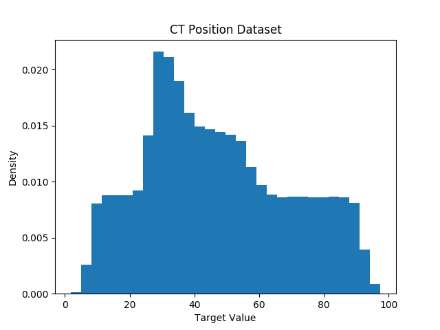
The CT Position dataset is from CT images of patients (Graf et al., 2011), with 385 features and the target set to the relative location of the image.
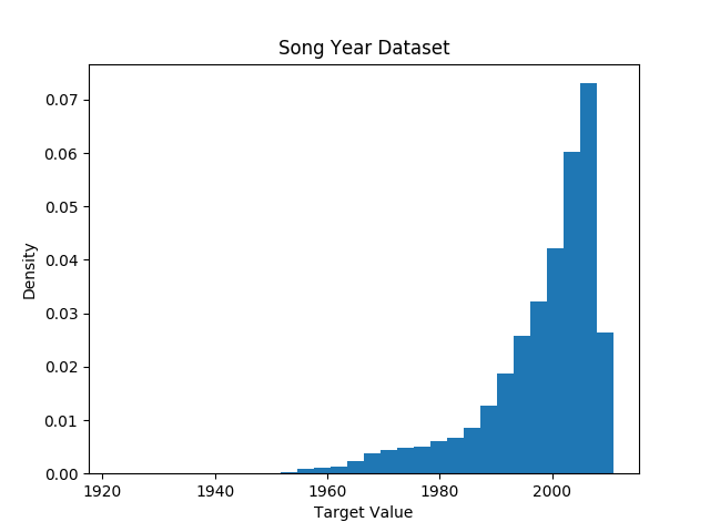
The Song Year dataset is a subset of The Million Song Dataset (Bertin-Mahieux et al., 2011), with 90 audio features for a song and target corresponding to the release year.
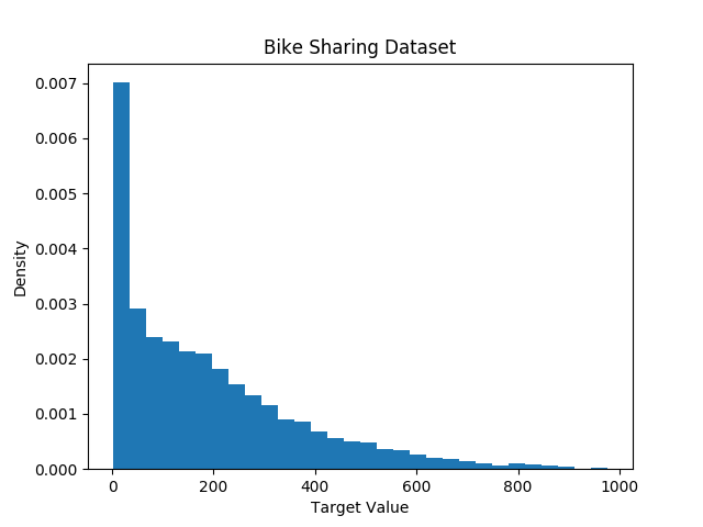
The Bike Sharing dataset (Fanaee-T and Gama, 2014), about hourly bike rentals for two years, has 16 features and target set to the number of rented bikes.
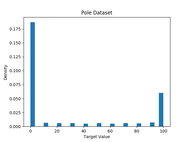
The Pole dataset (Olson et al., 2017), describes a telecommunication problem and has 49 features.

All datasets are complete and there is no need for data imputation. All features are transformed to have zero mean and unit variance. We randomly split the data into train and test sets in each run. Root mean squared error (RMSE) and mean absolute error (MAE) are reported over 5 runs, with standard errors. Other ways of processing these datasets may result in a higher performance. The goal of this study, however, is comparing different methods and testing hypotheses rather than achieving state-of-the-art results on these tasks. More details about these datasets are provided in Table 6 and Figure 12 in the appendix. We will show the results on CT Position dataset in the main paper and defer the results on the other datasets to Appendix C.

4.3 Algorithms

We compared several regression strategies, distribution learning approaches and several variants of HL. All the approaches—except for Linear Regression—use the same neural network, with differences only in the output layer. Unless specified otherwise, all networks using HL have 100 bins. The support of the histogram is chosen by the dataset target range and 10 bins are kept for padding on each side to minimize the effect of truncation. Hyperparameters for comparison algorithms are chosen according to the best Test MAE. Network architectures were chosen according to best Test MAE for $\ell_{2}$. More details about the architectures and the range of hyperparameters are provided in Appendix C.
Linear Regression is included as a baseline, using ordinary least squares with the inputs.
Squared-error $\ell_{2}$ is the neural network trained using the $\ell_{2}$ loss. The targets are normalized to range $[0,1]$, which was needed to improve stability and accuracy.
$\mathbf{\ell_{2}}$+Noise is the same as $\ell_{2}$, except Gaussian noise is added to the targets as a form of augmentation.
$\mathbf{\ell_{2}}$+Clipping is the same as $\ell_{2}$, but with gradient norm clipping during training.
Absolute-error $\ell_{1}$ is the neural network trained using the $\ell_{1}$ loss.
MDN is a Mixture Density Network (Bishop, 1994) that models the target distribution as a mixture of Gaussian distributions.
$\mathbf{\ell_{2}}$+Softmax uses a softmax-layer with $\ell_{2}$ loss, $\sum_{i=1}^{k}(f_{i}(\mathbf{x}_{j})m_{i}-y_{j})^{2}$ for bin centers $m_{i}$, with otherwise the same settings as HL-Gaussian.
HL-OneBin is HL, with Dirac delta target distribution.
HL-Uniform is HL, with a target distribution that mixes between a delta distribution and the uniform distribution, with a weighting of $\epsilon$ on the uniform and $1-\epsilon$ on the delta.
HL-Gaussian is HL, with a truncated Gaussian distribution as the target distribution. The parameter $\sigma$ is set to the width of the bins. Importantly, we do not tune any of HL-Gaussian’s hyperparameters to individual datasets.

4.4 Overall Results

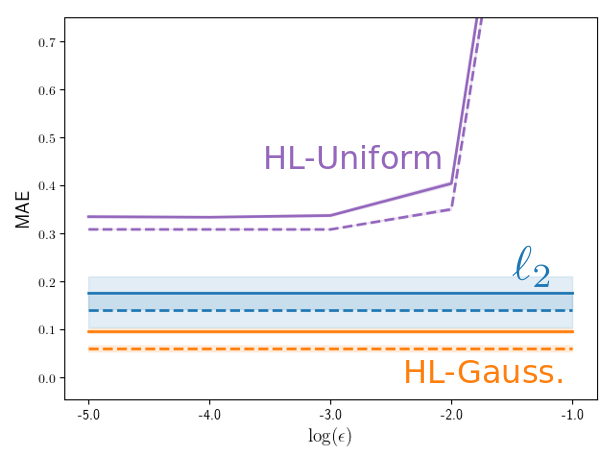
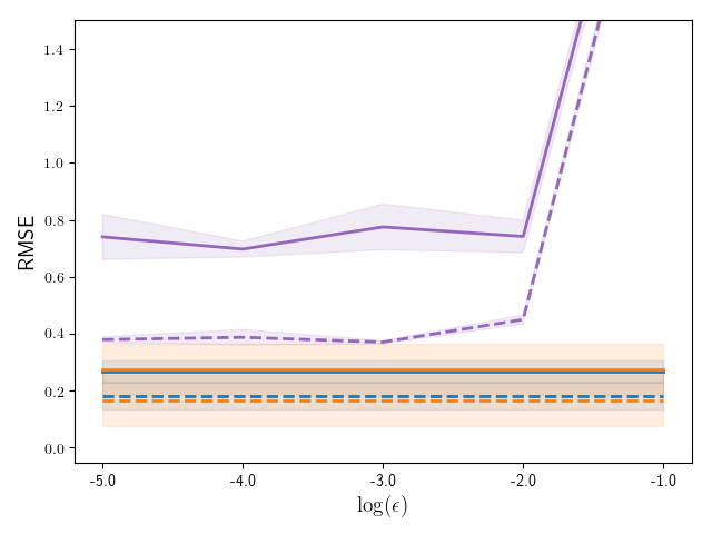
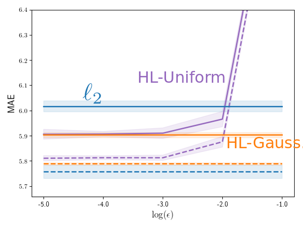
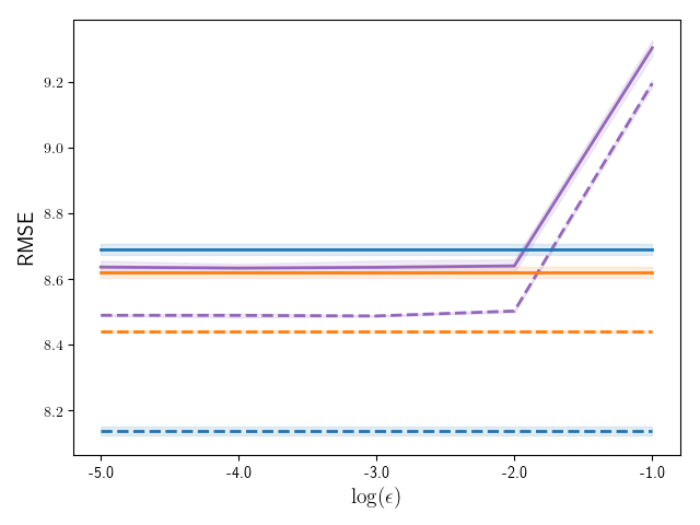
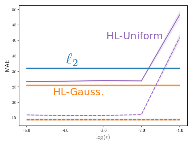
We first report the relative performance of different baselines compared to HL-Gaussian in Table 1. The error rates of HL-Uniform are plotted separately in Figure 3 to show that, regardless of the choice of the parameter in the loss, a uniform target distribution cannot help performance. We focus on Test MAE as the evaluation criterion due to considerably lower variability in the results and its wide use in practice and present Train MAE, Train RMSE, and Test RMSE to provide a complete picture.

Method	Train MAE	Train RMSE	Test MAE	Test RMSE
Lin Reg	$6.073$$(\pm 0.007)$	$8.209$$(\pm 0.006)$	$6.170$$(\pm 0.025)$	$8.341$$(\pm 0.025)$
$\ell_{2}$	$0.140$$(\pm 0.036)$	$0.183$$(\pm 0.048)$	$0.176$$(\pm 0.034)$	$0.267$$(\pm 0.039)$
$\ell_{2}$+Noise	$0.114$$(\pm 0.011)$	$0.152$$(\pm 0.015)$	$0.152$$(\pm 0.010)$	$0.311$$(\pm 0.076)$
$\ell_{2}$+Clip	$0.111$$(\pm 0.004)$	$0.143$$(\pm 0.005)$	$0.148$$(\pm 0.004)$	$0.231$$(\pm 0.006)$
$\ell_{1}$	$0.121$$(\pm 0.007)$	$0.164$$(\pm 0.007)$	$0.162$$(\pm 0.006)$	$0.389$$(\pm 0.038)$
MDN	$0.114$$(\pm 0.004)$	$0.152$$(\pm 0.005)$	$0.153$$(\pm 0.004)$	$0.308$$(\pm 0.035)$
$\ell_{2}$+softmax	$0.065$$(\pm 0.006)$	$0.094$$(\pm 0.008)$	$0.105$$(\pm 0.006)$	$0.301$$(\pm 0.067)$
HL-OneBin	$0.309$$(\pm 0.000)$	$0.364$$(\pm 0.006)$	$0.335$$(\pm 0.004)$	$0.660$$(\pm 0.099)$
HL-Gauss.	$0.061$$(\pm 0.006)$	$0.164$$(\pm 0.090)$	$0.098$$(\pm 0.005)$	$0.274$$(\pm 0.090)$

Table 1: Overall results on CT Scan. HL-Gaussian achieved the lowest Test MAE. Among the other methods, $\ell_{2}$+softmax yielded an error rate close to that of HL-Gaussian, and the rest of the baselines performed worse. There was a large gap between the performance of HL-OneBin and HL-Gaussian.

The overall conclusions are that HL-Gaussian does not harm performance and can often considerably improve performance over alternatives.

Another observation is that simply modeling the output distribution cannot achieve HL-Gaussian’s performance. This is made clear by comparing HL-Gaussian and MDN. MDN learns the output distribution but as a mixture of Gaussian components rather than a histogram. In our experiments MDN consistently underperformed HL-Gaussian. Note that the error rate reported for MDN is the one observed after fixing numerical instabilities and tuning the number of components.

A related idea to learning the distribution explicitly is to use data augmentation in the target space as an implicit approach to minimizing divergences to distributions. We therefore also compared to directly modifying the labels and gradients, with $\ell_{2}$-Noise and $\ell_{2}$-Clipping. These model do perform slightly better than Regression for some settings, but do not achieve the same gains as HL-Gaussian. The conclusion is that HL-Gaussian’s performance cannot be attributed to data augmentation in the targets.

Figure 3: HL-Uniform results on CT Scan. Dotted and solid lines show train and test errors respectively. The parameter $\epsilon$ is the weighting on the uniform distribution and raising it only impaired performance.

A well-known weakness of the $\ell_{2}$ loss is its sensitivity to outliers. To find if the difference between the performance of the $\ell_{2}$ loss and HL-Gaussian can be explained by the presence of outliers in the dataset, we can compare HL-Gaussian with the $\ell_{1}$ loss which is robust to outliers. The model trained with $\ell_{1}$ still underperformed HL-Gaussian on three datasets, which suggests that the gap between the performance of HL-Gaussian and the $\ell_{2}$ loss is not merely due to the presence of outliers in the dataset. Further experiments with other robust losses can provide a clearer conclusion.

Choices of target distribution other than a Gaussian distribution are not effective. HL-OneBin and HL-Uniform appear to have less advantages, as shown in the results, and both can actually do worse than $\ell_{2}$. A uniform target distribution on all the datasets only worsened the error. An important artifact of label smoothing in HL-Uniform is that it biases the mean of the distribution. Since the mean of a uniform distribution is the center of the range, mixing the target distribution with a uniform distribution pulls the mean towards the center of the range. Recall from Section 3 that HL will suffer from large bias if the mean of the target distribution is far from the target.

Finally, $\ell_{2}$+softmax performed close to HL-Gaussian on the CT Position dataset and slightly worse on the other tasks. While this model does not estimate the target distribution by minimizing the KL-divergence, it still benefits from the softmax nonlinearity in the output layer like HL-Gaussian. The comparison between $\ell_{2}$+softmax and HL-Gaussian shows that this softmax nonlinearity appears to be beneficial but it cannot totally explain HL-Gaussian’s performance. In our experiments on the three other datasets in Appendix E $\ell_{2}$+softmax consistently underperformed HL-Gaussian.

The comparisons in this section address several questions regarding HL-Gaussian’s performance. HL-Gaussian can often work better than $\ell_{2}$, and this rise in performance cannot be solely attributed to learning a flexible distribution, using data augmentation in the labels, being robust to outliers in the dataset, or employing a softmax nonlinearity in the model.

4.5 Bias and the Choice of Target Distribution

Characterizing the discretization bias in section 3 showed a link between the bias of the loss and the choice of $\sigma$ in HL-Gaussian. This parameter can also affect the bias from truncation as it controls the probability in the tails of the target distribution that exceeds the support of the histogram. This section empirically investigates the effect of the target distribution on the bias of the loss. We first show how different values of $\sigma$ result in different levels of bias. Then, we compare the target distributions of HL-Gaussian and HL-OneBin with another target distribution which reduces the bias to zero. Finally, we evaluate HL-OneBin and HL-Gaussian using different parameter values to find if these parameters control a bias-variance trade-off.

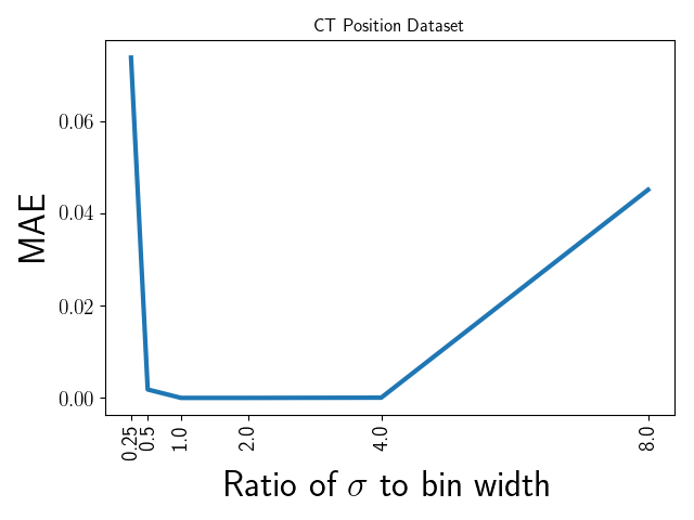
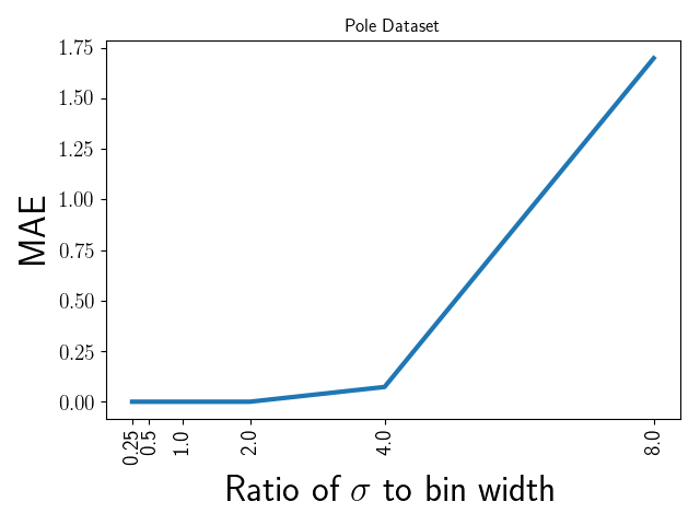
Weightings in HL-Gaussian (which represent the area under of the target distribution’s pdf in the range of each bin) are computed before the training, and the histogram is trained to mimic these weightings. To obtain low bias, we want the mean of the trained histogram to be close to the original target. To analyze how close the loss is to this situation in practice, we plot the mean absolute error between the original targets in our datasets and the mean of the histograms that perfectly match weightings obtained from those targets. Figure 4 shows this error for HL-Gaussian with 100 bins and different choices of $\sigma$.

Figure 4: MAE between the means of HL targets and the original labels. It can be seen that extreme values of $\sigma$ on either side biased the mean of the target distributions.

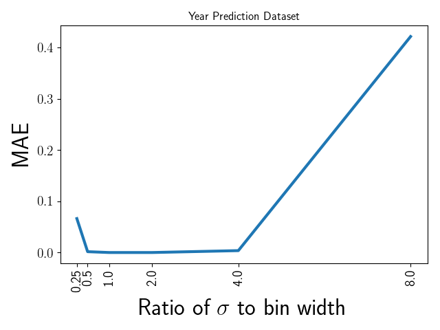
This simple analysis suggests that choosing a Gaussian target distribution with a carefully tuned variance parameter (rather than Dirac delta) can come with the extra benefit of reducing bias. To see to what extent the gap between HL-OneBin and HL-Gaussian’s performance is because of this bias and to find if histogram losses in general are suffering from a large bias, we introduce a target distribution that reduces the discretization bias to zero (regardless of the number of bins) and compare it to HL-OneBin and HL-Gaussian in the ordinary setting of 100 bins. As we showed in Section 3, if the target distribution $q_{y}$ is chosen so that, for each sample, the expected value of the closest histogram density to it is exactly $y$, discretization bias is zero. Assume $m_{i}$ is the last bin center before $y$ (so $y$ is somewhere between $m_{i}$ and $m_{i+1}$). The idea is to use a histogram density with probability $1-\frac{y-m_{i}}{w}$ in bin $i$ and probability $\frac{y-m_{i}}{w}$ in bin $i+1$ as the target distribution. The expected value of this target distribution is always $y$ so this target distribution eliminates discretization bias. We call the Histogram Loss with this choice of target distribution HL-Projected and compare it with HL-OneBin and HL-Gaussian on the four datasets.

Method	CT Scan	Song Year	Bike Sharing	Pole
HL-OneBin	$0.335$$(\pm 0.004)$	$5.906$$(\pm 0.020)$	$26.689$$(\pm 0.280)$	$1.264$$(\pm 0.019)$
HL-Projected	$0.103$$(\pm 0.003)$	$5.917$$(\pm 0.019)$	$26.180$$(\pm 0.348)$	$0.741$$(\pm 0.018)$
HL-Gauss.	$0.098$$(\pm 0.005)$	$5.903$$(\pm 0.010)$	$25.525$$(\pm 0.331)$	$0.714$$(\pm 0.024)$

Table 2: Discretization bias experiment. The reported numbers are Test MAE. HL-Projected achieved a Test MAE close to that of HL-Gaussian, and performed noticeably better than HL-OneBin. The gap between HL-Gaussian and HL-Projected is small but appears on all the four datasets.

While the difference between the performance of HL-Projected and HL-Gaussian is small, it is consistent on the four datasets. The comparison shows that using this target distribution instead of HL-OneBin often results in a noticeable reduction in the errors, but the performance of HL-Gaussian remains unbeaten. Although HL-Projected removes discretization bias, it still does not have HL-Gaussian’s desirable property of punishing faraway predictions more severely. We also experimented with a variant of HL-Gaussian that adjusts the target distribution to remove any remaining bias but did not see any improvement. This is because the bias of HL-Gaussian with proper $\sigma$ and padding is negligible as discussed in Appendix B.

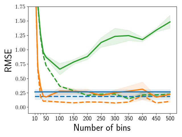
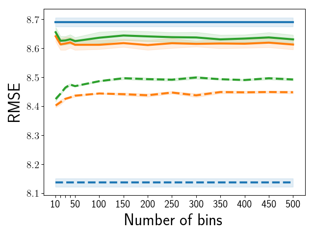
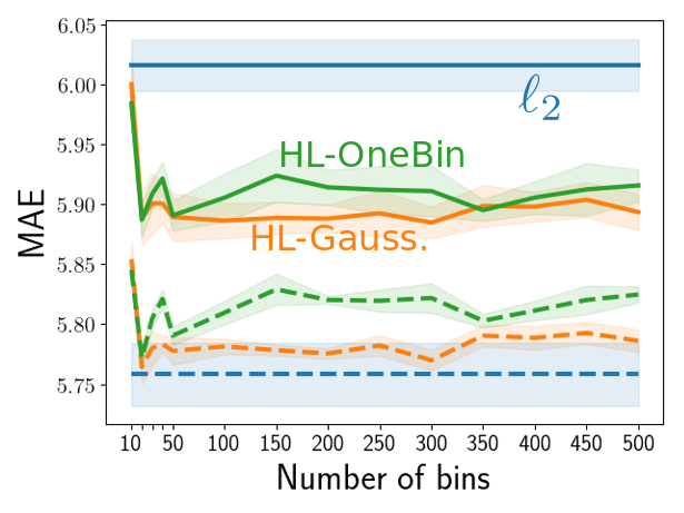
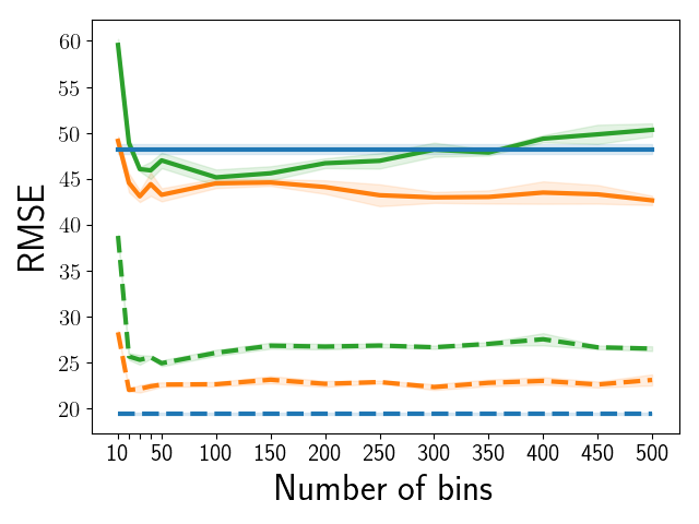
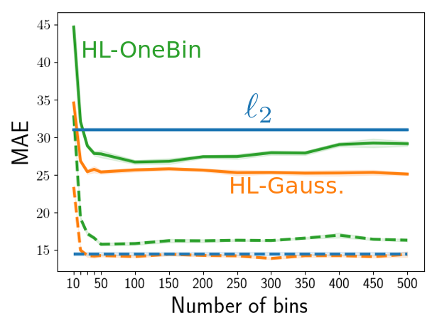
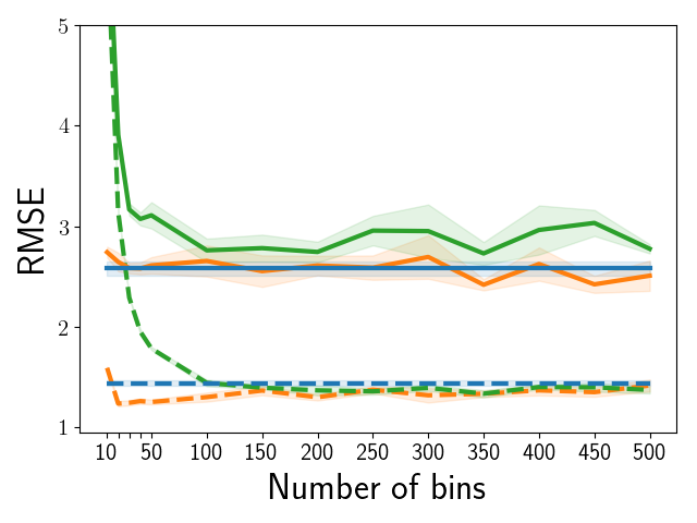
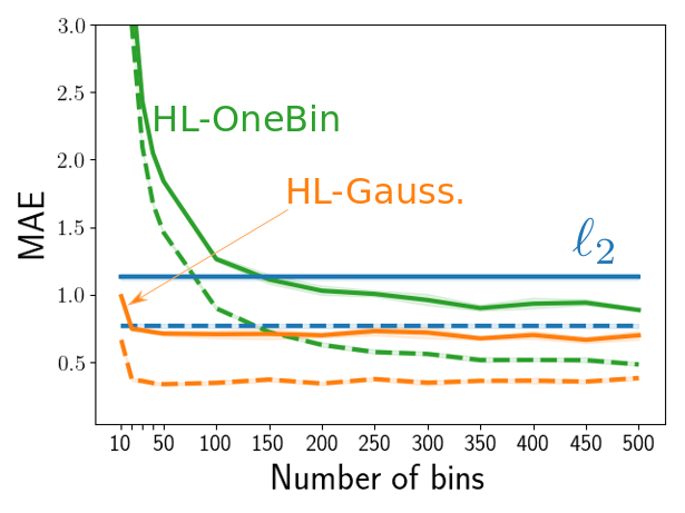
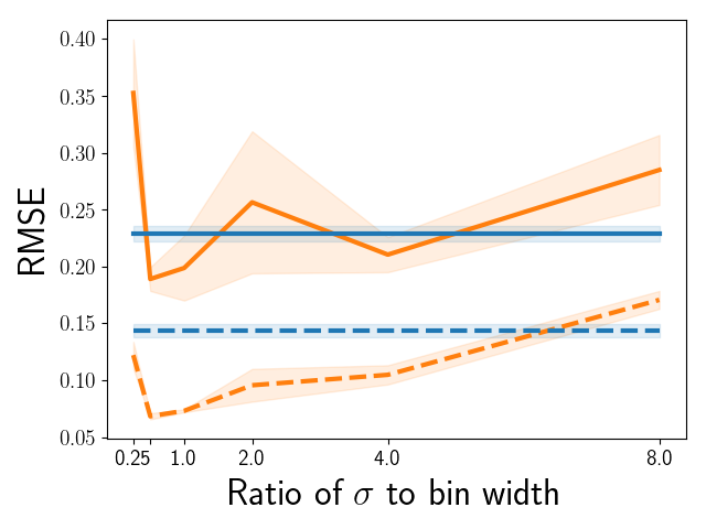
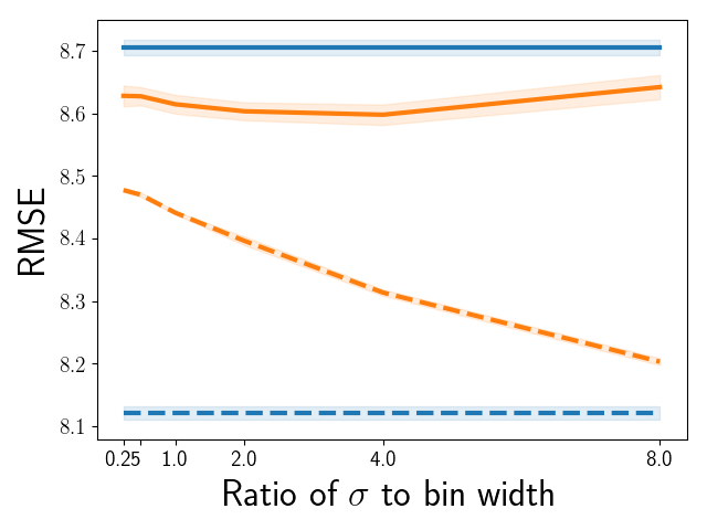
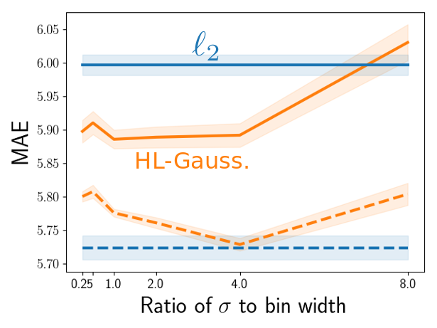
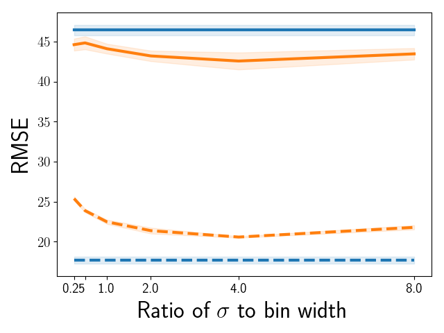
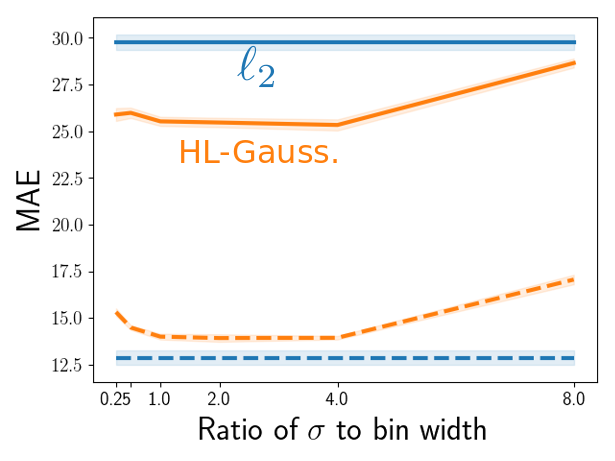
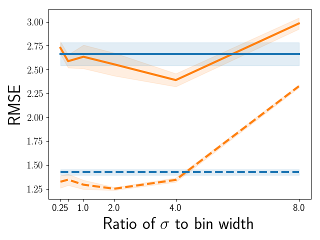
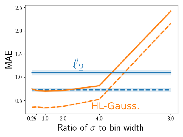
The parameters in the loss, namely the number of bins and $\sigma$, can affect the bias. A hypothesis is that a good choice of parameters for HL can reduce overfitting and place the method in a sweet spot in a bias-variance trade-off. Two experiments were designed to find if there is a bias-variance trade-off at work. In the first experiment we changed the number of bins while keeping the padding and target distribution $\sigma$ fixed. The second experiment studies the effect of changing $\sigma$ on the performance of HL-Gaussian. Figure 5 (Left) evaluates HL-Gaussian and HL-OneBin with different numbers of bins, and Figure 5 (Right) shows the effect of changing $\sigma$ on HL-Gaussian.

Figure 5: (Left) Changing the number of bins on CT Scan. Dotted and solid lines show train and test errors respectively. The performance of $\ell_{2}$ is shown as a horizontal line for comparison. A small number of bins resulted in high train and test errors, indicating high bias. A higher number of bins generally did not result in a rise in test error, with the exception of HL-OneBin’s test RMSE in Appendix E. (Right) Changing the parameter $\sigma$ on CT Scan. Extreme values of $\sigma$ resulted in bad performance. The error rates for train and test followed each other when changing this parameter.

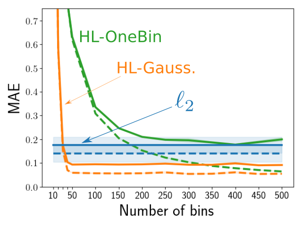
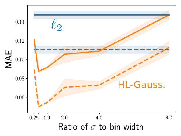
Evaluating different numbers of bins shows that, although the quality of solution deteriorates when the bins are too few, there is no sign of overfitting in HL-Gaussian with a higher number of bins. In the experiment on the $\sigma$ parameter, we observe a v-shaped pattern. Increasing $\sigma$ at first reduces both the train and test errors and, after a point, both errors begin to rise. Target distributions with higher $\sigma$ have longer tails and these high errors can be the result of truncation. Still, if a bias-variance trade-off was present, changing this parameter would generally result in decreasing the train error while increasing the test error in regions of low-bias and high-variance. This trend rarely exists in the results.

The analysis in this section shows the effect of the target distribution and the parameters of HL on the bias of the loss. Most of the gap between the performance of HL-Gaussian and HL-OneBin can be explained by the high bias of HL-OneBin. Both the number of bins and $\sigma$ can affect the bias of HL, but reducing this bias generally does not result in overfitting.

4.6 Representation

Learning a distribution, as opposed to a single statistic, provides a more difficult target—one that could require a better representation. The hypothesis is that amongst the functions $f$ in the function class $\mathcal{F}$, there is a set of functions that can predict the targets almost equally well. To distinguish amongst these functions, a wider range of tasks can make it more likely to select the true function, or at least one that generalizes better. We conducted three experiments to test the hypothesis that an improved representation is learned.

First, we trained with HL-Gaussian and $\ell_{2}$, to obtain their representations. We tested (a) swapping the representations and re-learning only the last layer, (b) initializing with the other’s representation, (c) and using the same fixed random representation for both. For (a) and (c), the optimizations for both are convex, since the representation is fixed. If the challenge of predicting a distribution in HL results in a better representation, one would expect the gap between $\ell_{2}$ and HL-Gaussian to go away when each one is trained on or initialized with the other’s representation. Table 3 shows the results.

	Loss	Default	Fixed	Initialized	Random
Train MAE	$\ell_{2}$	$0.140$$(\pm 0.036)$	$2.490$$(\pm 0.094)$	$0.148$$(\pm 0.013)$	$9.233$$(\pm 0.157)$
Train MAE	HL-Gauss.	$0.061$$(\pm 0.006)$	$0.153$$(\pm 0.020)$	$0.063$$(\pm 0.002)$	$2.604$$(\pm 0.103)$
Train RMSE	$\ell_{2}$	$0.183$$(\pm 0.048)$	$3.465$$(\pm 0.158)$	$0.205$$(\pm 0.022)$	$12.247$$(\pm 0.172)$
Train RMSE	HL-Gauss.	$0.164$$(\pm 0.090)$	$0.219$$(\pm 0.027)$	$0.085$$(\pm 0.004)$	$5.756$$(\pm 0.232)$
Test MAE	$\ell_{2}$	$0.176$$(\pm 0.034)$	$2.537$$(\pm 0.089)$	$0.185$$(\pm 0.013)$	$9.305$$(\pm 0.191)$
Test MAE	HL-Gauss.	$0.098$$(\pm 0.005)$	$0.187$$(\pm 0.019)$	$0.101$$(\pm 0.002)$	$2.727$$(\pm 0.113)$
Test RMSE	$\ell_{2}$	$0.267$$(\pm 0.039)$	$3.551$$(\pm 0.143)$	$0.299$$(\pm 0.025)$	$12.315$$(\pm 0.216)$
Test RMSE	HL-Gauss.	$0.274$$(\pm 0.090)$	$0.287$$(\pm 0.024)$	$0.183$$(\pm 0.005)$	$6.065$$(\pm 0.234)$

Table 3: Representation results on CT Scan. We tested (a) swapping the representations and re-learning on the last layer (Fixed), (b) initializing with the other’s representation (Initialized), (c) and using the same fixed random representation for both (Random) and only learning the last layer. Using HL-Gaussian representation for $\ell_{2}$ (first column, Fixed) caused a sudden spike in error, even though the last layer in $\ell_{2}$ was re-trained. This suggests the representation is tuned to HL-Gaussian. The representation did not even seem to give a boost in performance, as an initialization (second column, Initialization). Finally, even with the same random representation, where HL-Gaussian cannot be said to improve the representation, HL-Gaussian still obtained substantially better performance.

The results above are surprisingly conclusive. Using the representation from HL-Gaussian does not improve performance of $\ell_{2}$, and even under a random representation, HL-Gaussian performs noticeably better than $\ell_{2}$.

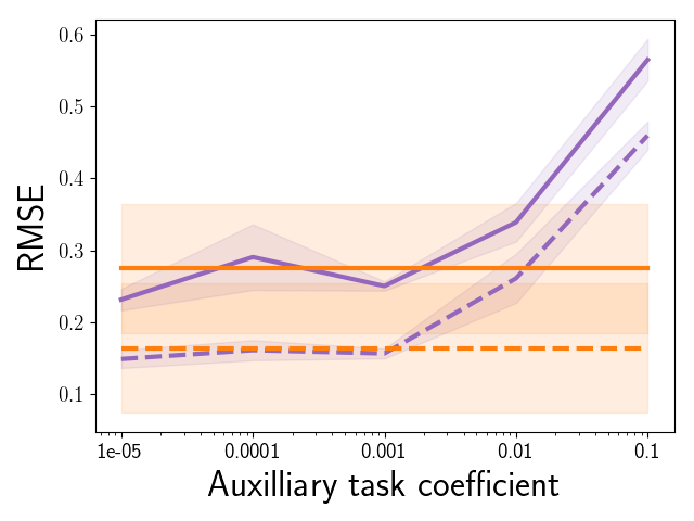
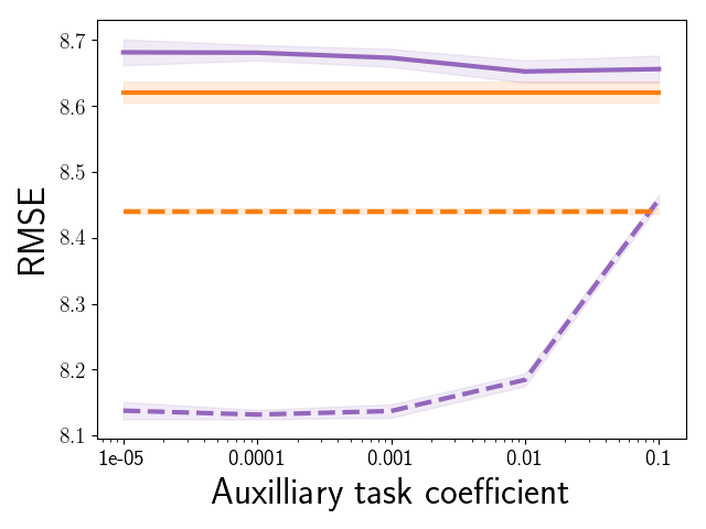
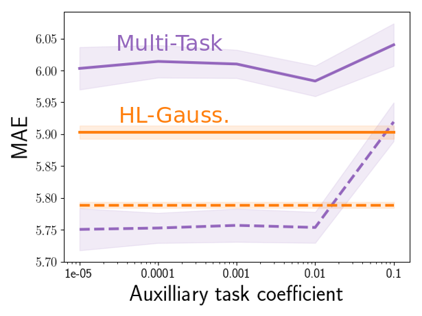
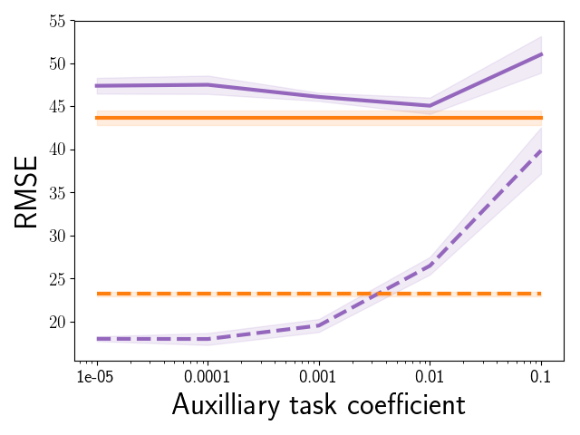
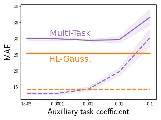
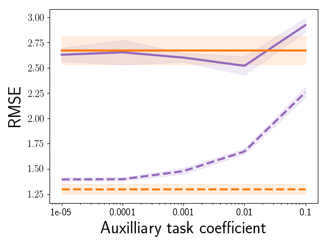
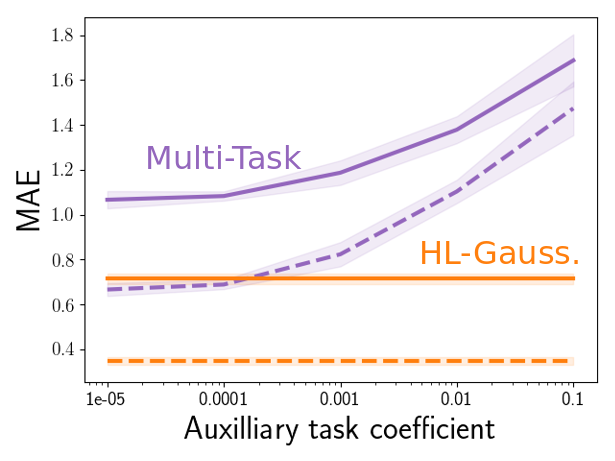
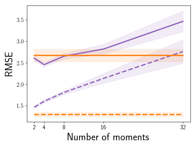
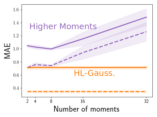
In the second experiment, we tested a network called Multi-Task that predicted both the expected value (with the $\ell_{2}$ loss) and the distribution (using HL-Gaussian). The predicted distribution was not used for evaluation and was only present during the training as an auxiliary task to improve the representation. If predicting the extra information in a distribution is the reason for the superior performance of HL-Gaussian, a regression network with the auxiliary task of predicting the distribution is expected to achieve a similar performance. Figure 6 (Left) shows the results on the four datasets.

It can be seen from these results that raising the coefficient for the auxiliary task does not improve the performance, and the new model generally has higher errors than HL-Gaussian. The conclusion is that the extra information required for predicting the distribution cannot explain the gap between the $\ell_{2}$ loss and HL-Gaussian.

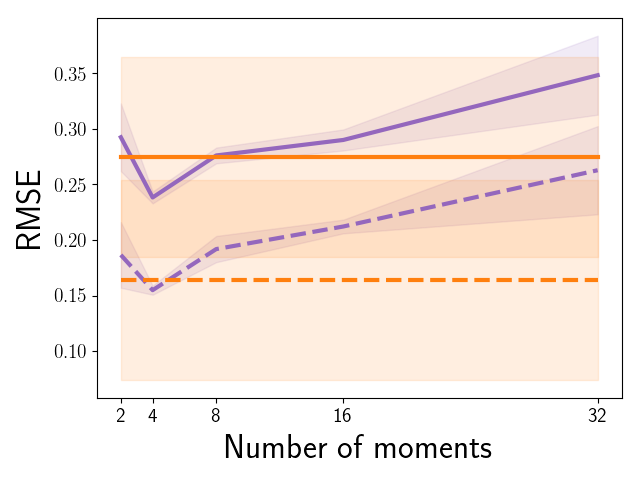
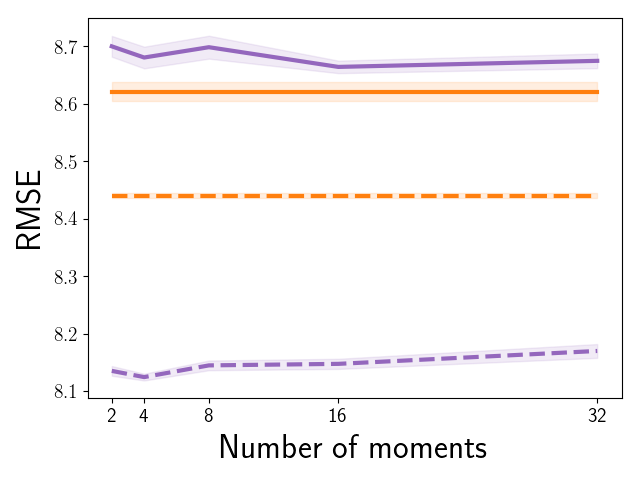
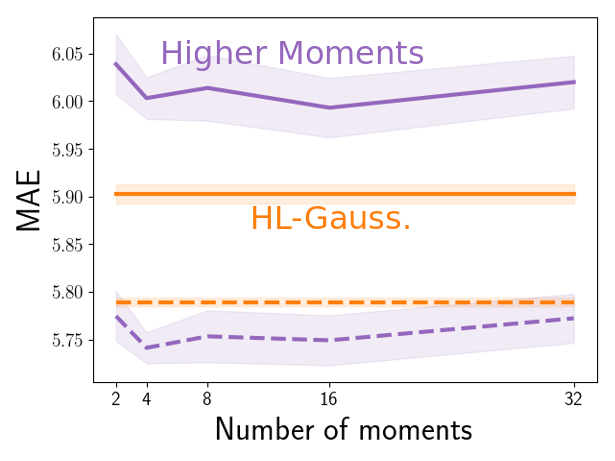
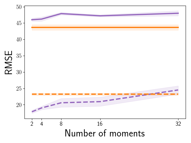
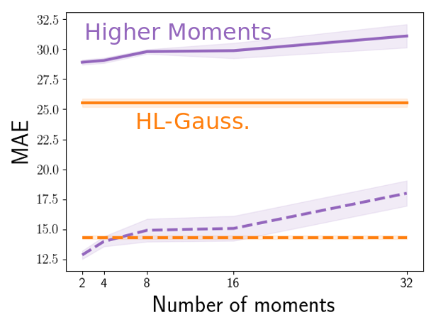
It might be argued that learning a histogram is not a suitable auxiliary task for regression, and the negative results above can be due to the incompatibility between predicting the mean with the $\ell_{2}$ loss and predicting the distribution with HL-Gaussian. We trained the $\ell_{2}$ model with another auxiliary task in the third experiment. For the new task, predicting higher moments of the distribution, the target is raised to higher powers and the extra outputs try to estimate it by reducing the $\ell_{2}$ loss. These auxiliary tasks of predicting higher moments are only used to improve the representation during training and are discarded at inference time. The results are shown in Figure 6 (Right).

Figure 6: (Left) Multi-Task Network results on CT Scan. The loss function is the mean prediction’s squared error plus the distribution prediction’s KL-divergence multiplied by a coefficient. The horizontal axis shows the coefficient for KL-divergence. Dotted and solid lines show train and test errors respectively. There was not a substantial drop in the error rate when increasing the coefficient in the loss and the performance only became worse. (Right) Higher Moments Network results on CT Scan. The horizontal axis shows the number of moments (including the mean). There was no substantial decrease in error when predicting higher moments. With four moments, there was a slight reduction in error but the new model still performed worse than HL-Gaussian in terms of Test MAE.

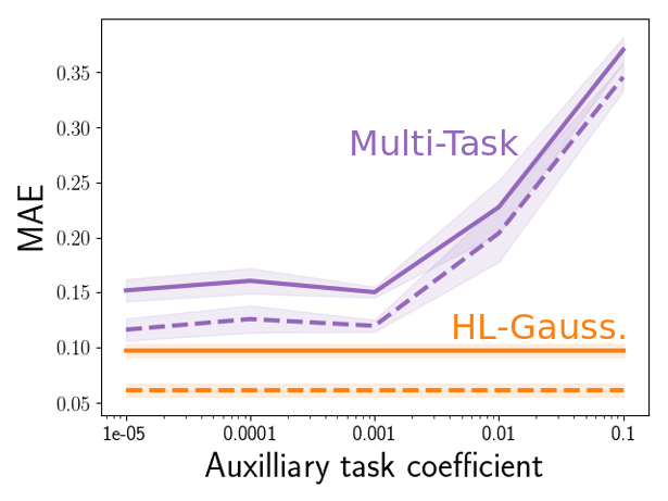
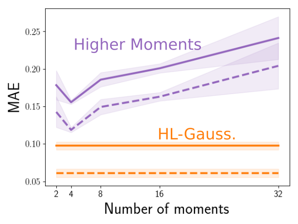
There is little gain in predicting higher moments and the new model still underperforms HL-Gaussian. Like the previous experiment, predicting this extra information about the output distribution appears to have little benefit as an auxiliary task.

The experiments in this section consistently reject the hypothesis that the challenge of predicting the distribution is the main factor behind HL-Gaussian’s performance. The performance cannot be achieved by exploiting HL-Gaussian’s representation or by predicting the histogram or higher moments of the distribution as auxiliary tasks.

4.7 Optimization Properties

In Section 3 we provided a bound on the gradient norm of HL that suggested ease of optimization with gradient descent. In this section we show two experiments that study the optimization of the $\ell_{2}$ loss and HL empirically.

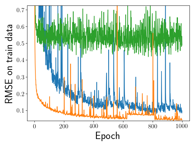
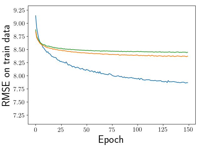
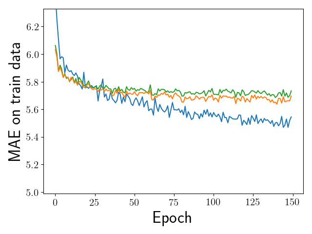
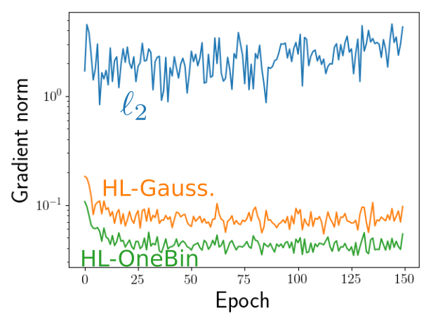
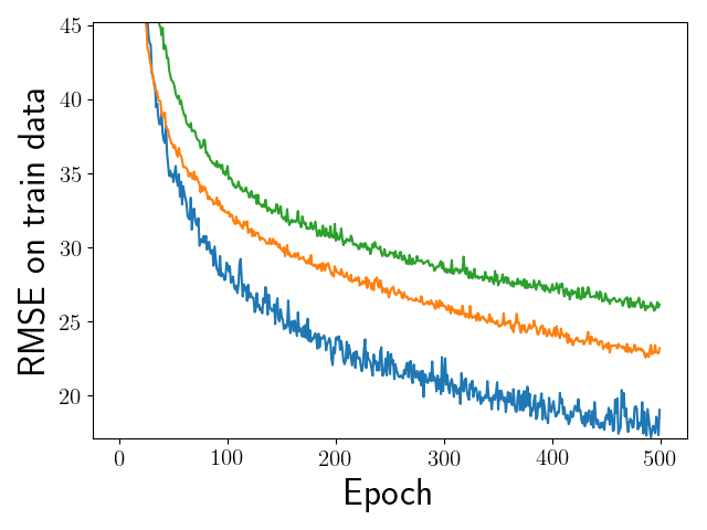
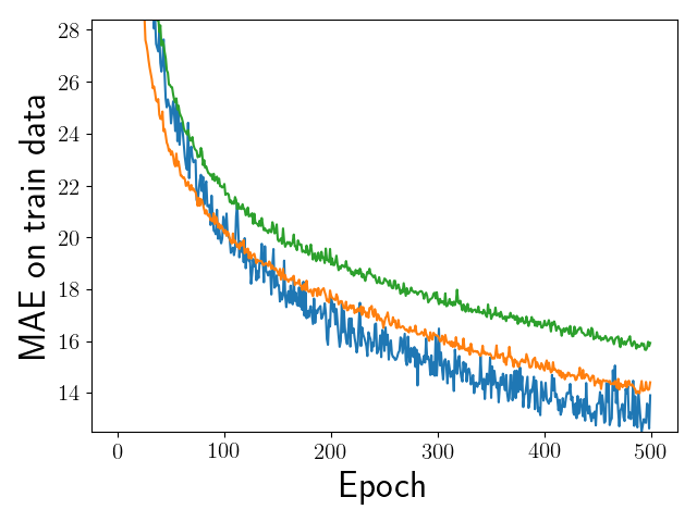
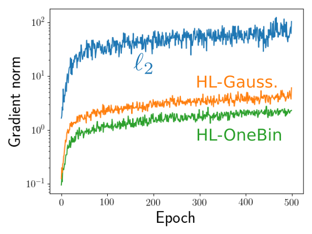
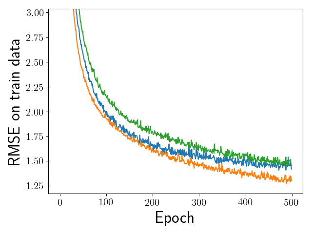
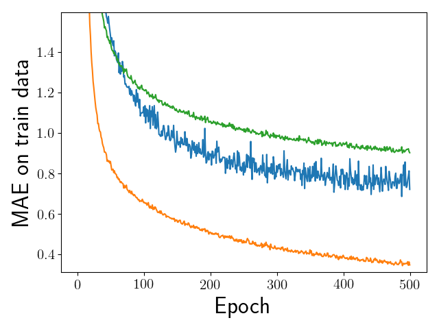
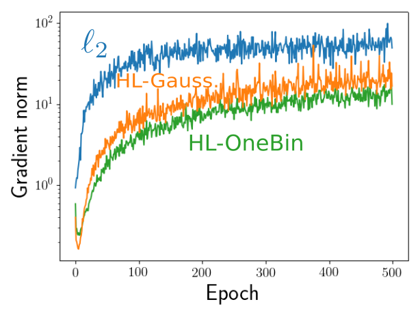
First, we recorded the training errors and gradient norms during training to see if using HL-Gaussian is beneficial for optimization. Each gradient norm value was normalized by the difference between the training loss observed at that point in the training of the model and the minimum possible value for the loss. The goal was to find which model trains faster and has a smoother loss surface. Without the normalization of gradient norms, a simple scaling of the loss would shrink the fluctuations of gradient norms in the plot without making the optimization easier. Figure 7 shows the results.

Figure 7: Training process on CT Scan. (Left) HL-Gaussian reduced the train errors much faster than $\ell_{2}$. (Right) The gradient norm of $\ell_{2}$ was highly varying through the training.

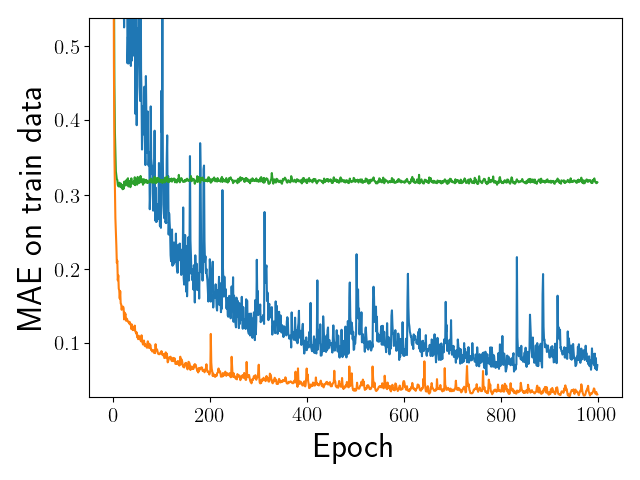
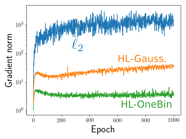
The results above suggests that HL-Gaussian shows more stable gradients than $\ell_{2}$ and generally reduces the loss by a large amount in the first few epochs. As discussed in Section 3, these properties can explain the performance of HL-Gaussian. In comparison with HL-OneBin, however, HL-Gaussian does not show a noticeable benefit in optimization.

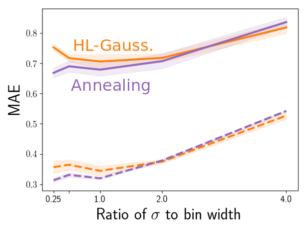
The second experiment explores the role of $\sigma$ in HL-Gaussian. The benefit of the parameter $\sigma$ in HL-Gaussian can be twofold: (1) improving the final solution and (2) improving optimization process. To compare the effect of these two properties, we design a network, called Annealing Network, that starts with a high $\sigma$ and gradually reduces it to a small $\sigma$ during the training. The initial $\sigma$ is $8$ times the bin width, and during the first $20\%$ of epochs the current value of $\sigma$ is multiplied by a constant $\tau$ at each epoch. The training continues without further annealing once $20\%$ of the epochs are finished. The assumption is that the effect of $\sigma$ on optimization shows up during the training, unlike the effect on final solution. Therefore, if the effect on optimization is substantial, the model that has a high $\sigma$ earlier in training can benefit from it despite its small $\sigma$ at the end. Results are shown in Figure 8.

Figure 8: Annealing results on (Left) CT Scan, (Middle) Song Year, and (Right) Bike Sharing. Dotted and solid lines show train and test errors respectively. The X-axis for Annealing shows the final value of $\sigma$. HL-Gaussian keeps $\sigma$ fixed to this value throughout training while Annealing starts with a higher value of $\sigma$ and reduces it to this value. There is some benefit in starting with a higher $\sigma$ and reducing it on song Year and Bike Sharing. See Appendix E for the other dataset and RMSE results.

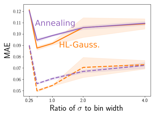
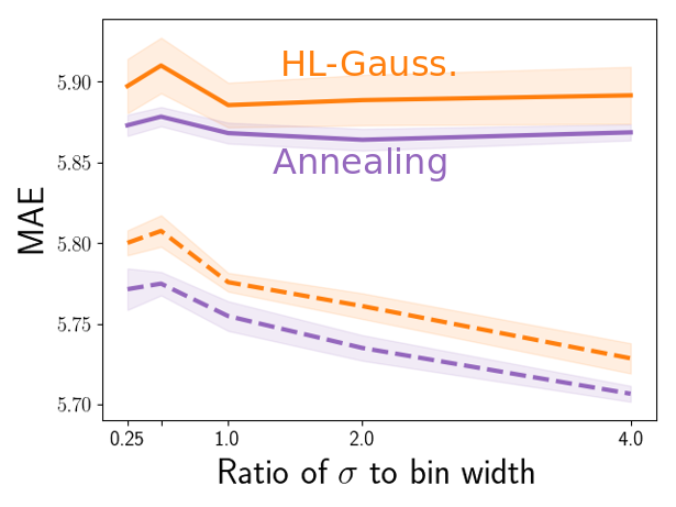
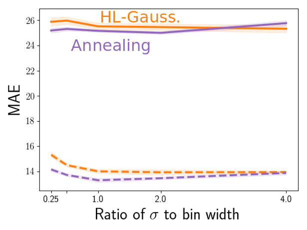
There was some gain in performance when the model started with a large value of $\sigma$ and then reached a small value through annealing compared to training with a fixed small value of $\sigma$. So the parameter $\sigma$ has some impact on the optimization.

The takeaway is that using HL instead of the $\ell_{2}$ loss helps with optimization, which confirms the previous observation by Imani and White (2018). Further, the choice of the target distribution and the parameter in the loss have some effect on the optimization.

4.8 Corrupted Targets and Input Perturbations

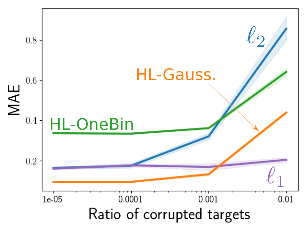
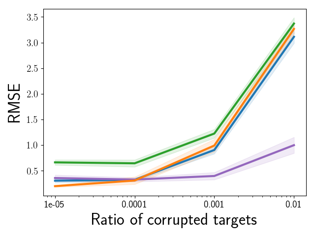
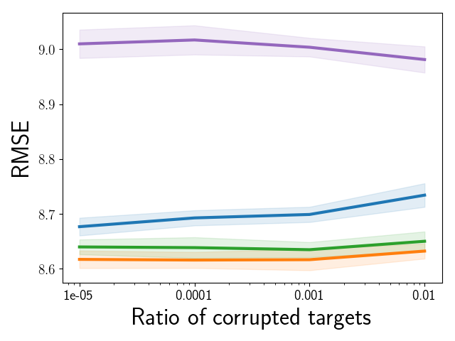
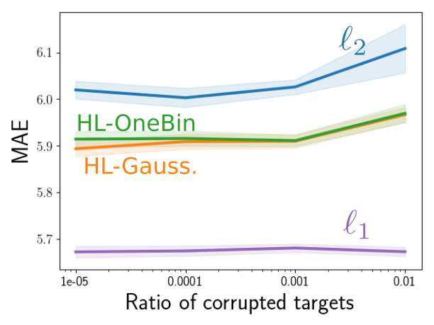
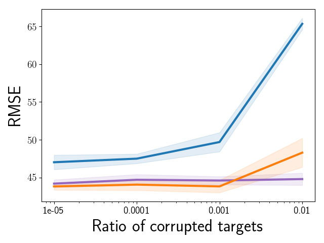
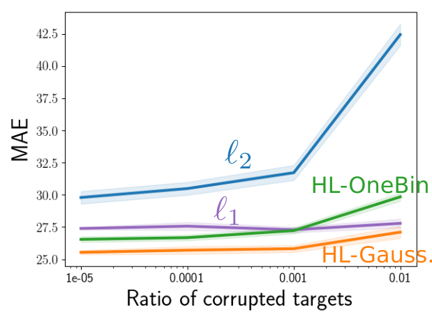
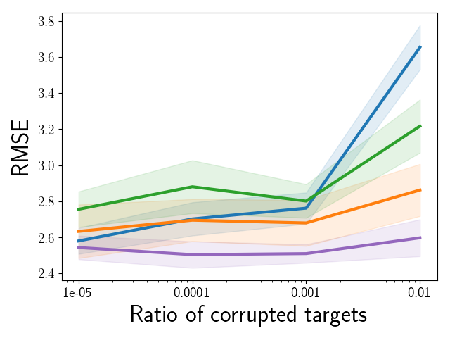
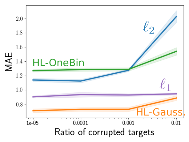
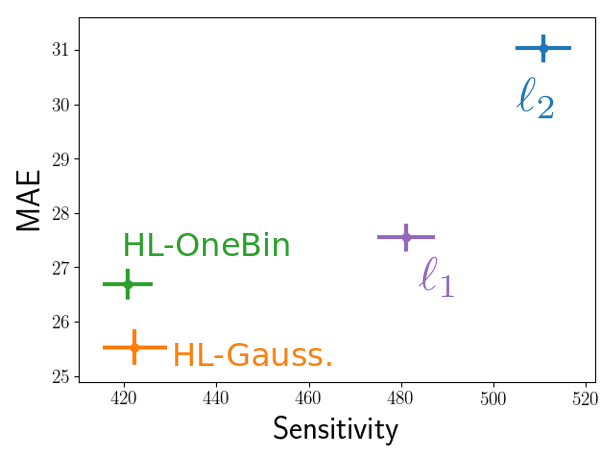
We first tested $\ell_{2}$ loss, $\ell_{1}$ loss, HL-OneBin, and HL-Gaussian on datasets with corrupted targets. At each level, we replaced a ratio of training targets with numbers sampled uniformly from the range of targets in the dataset. Results in Figure 9 (Left) show that HL-Gaussian and HL-OneBin are more robust to corrupted targets than $\ell_{2}$ but not as robust as $\ell_{1}$.

These results show a situation where the difference between the performance of HL and the $\ell_{2}$ loss is more pronounced. Interestingly, HL can work worse than the $\ell_{1}$ loss in the presence of corrupted targets. This analysis is exploratory, and further studies on the effect of corrupted targets in training can lead to a better understanding the differences between these loss functions.

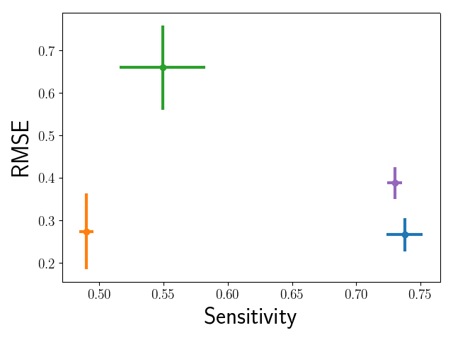
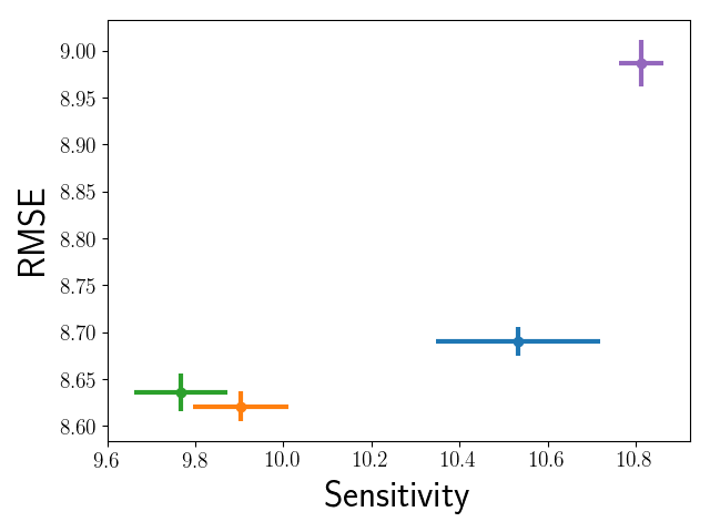
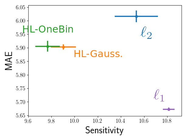
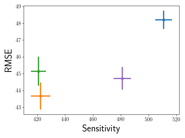
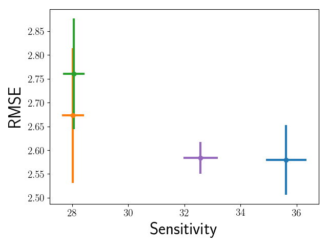
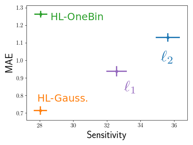
We then compared the sensitivity of the outputs of models trained with $\ell_{2}$ loss, $\ell_{1}$ loss, HL-OneBin, and HL-Gaussian to input perturbations. The measure we used was the Frobenius norm of the Jacobian of the model’s output w.r.t. the input. Predictions in a regression problem are scalar values, so the Jacobian becomes a vector whose elements are the derivative of the output w.r.t. each input feature. A high value of this measure means that a slight perturbation in inputs will result in a drastic change in output. For a classification problem, there are theoretical and empirical results on the connection of this measure and generalization (Novak et al., 2018; Sokolić et al., 2017). Also, a representation that is less sensitive to input perturbations with this measure has been shown to improve the performance of classifiers (Rifai et al., 2011). Following Novak et al. (2018), we evaluated this measure at the test points and reported the average. Figure 9 (Right) summarizes the results.

Figure 9: (a) Corrupted targets on CT Scan. The lines show test errors. The $\ell_{1}$ loss was robust to corrupted targets, and the $\ell_{2}$ loss was affected the most. (b) Sensitivity results on CT Scan. The horizontal axis shows the sensitivity of the model’s output to input perturbations (left means less sensitive) and the vertical axis shows the test error (lower is better). HL-Gaussian showed less sensitivity and lower test errors than $\ell_{1}$ and $\ell_{2}$.

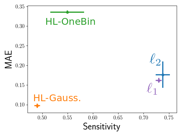
The results indicate that predictions of the models that are trained with HL are less sensitive to input perturbations than the ones trained with $\ell_{1}$ or $\ell_{2}$. Further analysis is required to know why this difference in sensitivity happens and to what extent it impacts the performance in a regression setting.

4.9 Summary of the Empirical Study

Through this section, we tested several hypotheses about the performance of HL. We found that

1. HL-Gaussian, even without careful parameter tuning, is a viable choice in regression and can often outperform the $\ell_{2}$ loss,

2. learning a flexible distribution is not why HL-Gaussian outperforms the $\ell_{2}$ loss,

3. data augmentation in the labels cannot explain the difference between the performance of HL-Gaussian and the $\ell_{2}$ loss,

4. robustness to outliers is not the reason why HL-Gaussian performs better,

5. the softmax nonlinearity in HL-Gaussian is beneficial but it cannot wholly explain its superior performance,

6. the choice of target distribution affects the bias of the loss and HL-OneBin can suffer from a high bias,

7. there is not a considerable bias-variance trade-off controlled by the number of bins and the $\sigma$ parameter,

8. predicting the full distribution does not force HL-Gaussian’s model to learn a better representation,

9. using HL-Gaussian instead of the $\ell_{2}$ loss helps gradient descent’s search for a good solution,

10. HL is more robust to corrupted targets in the dataset than the $\ell_{2}$ loss and less robust than the $\ell_{1}$ loss, and

11. HL finds a model whose output is less sensitive to input perturbations than both the $\ell_{2}$ loss and the $\ell_{1}$ loss.

5 Applications

This section explores the applicability of the HL-Gaussian beyond the previous simple regression datasets. We evaluate several network architectures on time-series prediction tasks using both HL-Gaussian and $\ell_{2}$ loss. The network choices include linear models, Long Short-Term Memory (LSTM) networks, and Transformers. We then extend the experiments to state-value prediction for Reinforcement Learning, where we evaluate the performance of both losses on the Atari prediction task.

5.1 Time Series Prediction

We use the Electricity Transformer Dataset (ETD, Zhou et al. (2021)) for the time series prediction experiments. The dataset contains $6$ features relating to the electricity loads, in addition to the oil temperature, which is the prediction target in all of our experiments. The data is collected from two different transformers and has two variants: hourly datasets, which were collected from each Transformer at an hourly rate, and 15-minute datasets, where the data collection happened $4$ times per hour.

We investigate the performance of three different network architectures on the four ET-Datasets. The three architectures are LSTM (Hochreiter and Schmidhuber, 1997b), Transformer (Vaswani et al., 2017) and a simple linear model as suggested by  Zeng et al. (2023). For each architecture, we had two variations, one trained with HL-Gaussian loss and one trained with $\ell_{2}$ loss. As a rule of thumb, we divide the output range to 100 bins, set $\sigma$ to twice this bin width, and then increase the bin width to add some padding as described in Appendix D. The same appendix section provides more details on the hyperparameters and the experiment setup.

Table 4 shows the results for all architectures on the four datasets. The results show that networks trained with HL-Gaussian achieved overall better performance across the different datasets and architectures.

Task	Architecture	Loss	Test MSE	Test MAE
ETTh1	Linear	$\ell_{2}$	$0.5288$	$0.589$
	Linear	HL-Gaussian	$0.3386$	$0.467$
	LSTM	$\ell_{2}$	$0.6067$	$0.6077$
	LSTM	HL-Gaussian	$0.1205$	$0.2693$
	Transformer	$\ell_{2}$	$0.08056$	$0.2123$
	Transformer	HL-Gaussian	$0.07822$	$0.208$
ETTh2	Linear	$\ell_{2}$	$0.6964$	$0.6544$
	Linear	HL-Gaussian	$0.2827$	$0.4283$
	LSTM	$\ell_{2}$	$0.2073$	$0.357$
	LSTM	HL-Gaussian	$0.1744$	$0.3302$
	Transformer	$\ell_{2}$	$0.1742$	$0.3324$
	Transformer	HL-Gaussian	$0.1582$	$0.3095$
ETTm1	Linear	$\ell_{2}$	$0.1197$	$0.2741$
	Linear	HL-Gaussian	$0.1167$	$0.2696$
	LSTM	$\ell_{2}$	$0.06158$	$0.1883$
	LSTM	HL-Gaussian	$0.06863$	$0.1977$
	Transformer	$\ell_{2}$	$0.04942$	$0.1711$
	Transformer	HL-Gaussian	$0.04272$	$0.1584$
ETTm2	Linear	$\ell_{2}$	$0.1708$	$0.3249$
	Linear	HL-Gaussian	$0.158$	$0.31$
	LSTM	$\ell_{2}$	$0.07258$	$0.2009$
	LSTM	HL-Gaussian	$0.04247$	$0.1505$
	Transformer	$\ell_{2}$	$0.1354$	$0.2863$
	Transformer	HL-Gaussian	$0.1239$	$0.2746$

Table 4: Time-series prediction results for different network architectures when trained with HL-Gaussian and $\ell_{2}$ losses. Switching from $\ell_{2}$ loss to HL-Gaussian consistently improves performance.

5.2 State Value Prediction

A central problem in Reinforcement Learning (RL) is state value prediction. An RL agent interacts with an environment modelled as a Markov Decision Process, and each action taken by the agent results in a transition, reward, and discounting or possible termination. The goal of state value prediction is to predict the expected sum of discounted future rewards from a state.

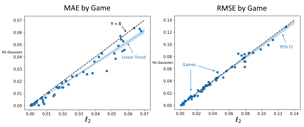
In our experiments, we predict state values for agents playing 58 different Atari 2600 games on the Arcade Learning Environment from Bellemare et al. (2013). In this setting, the state is observed through frames from the screen and the reward is based on the game score obtained. We use actions from the Atari Prediction Benchmark from Javed et al. (2023). This benchmark contains at least 10 million actions for each game. The actions were produced by a pre-trained rainbow DQN agent from the ChainerRL model zoo (Fujita et al., 2021). While the benchmark paper explores the partially-observable setting with a single frame per observation, we use a stack of 4 frames to make it fully-observable. For HL-Gaussian, the bin width is computed using Equation (16). Again, we divide the output range to 100 bins, set $\sigma$ to twice this bin width, and then increase the bin width to add some padding as described in Appendix D. We use the first 5% of the episodes as the test set and train the models for one epoch on the remaining episodes. We exclude 3 games from our analysis in which the agent received no rewards (namely Tennis, Venture, and Montezuma Revenge).

Table 5 contains the mean metrics obtained by HL-Gaussian and $\ell_{2}$ models over the 55 remaining games. HL-Gaussian outperformed $\ell_{2}$ in all metrics. The differences in both test RMSE and test MAE are statistically significant at $\alpha=0.05$ with p-values of $0.0294$ and $2.1199\times 10^{-6}$ respectively after applying a log-transform. These differences can be seen in Figure 10.

Loss	Train RMSE	Train MAE	Test RMSE	Test MAE
$\ell_{2}$	0.0295	0.0160	0.0418	0.0235
HL-Gaussian	0.0295	0.0141	0.0408	0.0199

Table 5: Mean Atari Results. HL-Gaussian generally results in lower errors.

Figure 10: Atari Results by Game. Points below the dashed black line are games where HL-Gaussian outperformed $\ell_{2}$, and the blue line is the zero-intercept linear trend.

6 Conclusion and Future Work

This section summarizes the contributions in the paper and highlights some future directions for research on this topic.

6.1 Contributions

We analyzed a recent approach to regression, the Histogram Loss (HL) (Imani and White, 2018), which consists of the KL-divergence between a flexible histogram prediction and target distributions. Experiments on a variety of datasets and networks showed that this loss function does not harm performance and, in fact, it often outperforms the oft-used $\ell_{2}$ loss with a fixed set of recommended hyperparameter values and without the need for careful hyperparameter sweeps. The recommended rule of thumb is using 100 evenly sized bins, setting $\sigma$ to twice the bin width, and then raising the bin width by three times $\sigma$ to create some padding.

Besides providing a solution for regression, HL offers a testbed for analyzing some of the open questions in previous work. A question that we explored in depth was one of the hypotheses put forward by Bellemare et al. (2017): whether the performance gap between a model that learns the full distribution and one that only estimates the mean can be attributed to their representations, in a manner analogous to multi-task learning. Our experiments suggest that this is not the case in regression. Instead, the bound on the gradient norm of HL as well as its stability during training hint at a better-behaved loss surface as an important factor in effect. An additional factor in HL’s performance is the softmax nonlinearity that models the histogram distribution as we found that a minimizing the $\ell_{2}$ loss between the target and the mean of a histogram distribution could yield an error rate close to that of HL.

Another question was the impact of the type of target distribution on performance. The method for constructing the target distribution has an effect on bias of the loss, and a Gaussian target distribution with a reasonable bandwidth can result in a lower bias than one-hot targets. However, it is also important to note that this is not the only benefit of a Gaussian target distribution, since even HL with an unbiased target distribution underperformed HL-Gaussian.

6.2 Future Work

Our results on the behavior of different models during optimization are still preliminary and a more in-depth investigation is needed for a crisp conclusion. There is a growing literature on understanding loss surfaces of neural networks. Theoretical analyses are often insightful but require strong assumptions on data or model (Soltanolkotabi et al., 2018; Choromanska et al., 2015; Jacot et al., 2018; Arora et al., 2018). An alternative line of research compares loss surfaces empirically by techniques like projection on lower dimensions or slightly perturbing the parameters in random directions often to compare the flatness of the solutions (Hochreiter and Schmidhuber, 1997a; Keskar et al., 2017; Li et al., 2018). There are three important challenges in performing such comparison. First, intuitions about optimization in low-dimensional surfaces do not necessarily transfer to higher dimensions. Second, sometimes (like when comparing HL and $\ell_{2}$ loss) the surfaces compared are of different dimensionalities, and this difference can be a confounding factor. Third, causal connection between the performance of the network and some measures of flatness is disputed as solutions with similar performance but varying levels of flatness can be easily constructed (Dinh et al., 2017).

Despite the challenges above, investigating possible connections between performance gains in distribution learning and flatness is promising. Training regimes and optimizers that implicitly or explicitly enforce flatness have shown better final performance, an initial phase of fast learning, higher robustness to some degree of label noise, and less sensitivity to input perturbations (Keskar et al., 2017; Hoffer et al., 2017; Foret et al., 2021; Jiang et al., 2020; Novak et al., 2018). In our empirical study HL-Gaussian showed the exact same properties in regression when compared with the $\ell_{2}$ loss.

The experiment settings and baselines in this paper were focused on singling out and studying the points of difference between HL and the $\ell_{2}$ loss. Further experiments can be designed to evaluate intersections of these factors. As a simple example, one could switch the $\ell_{2}$ loss to the $\ell_{1}$ loss in our $\ell_{2}$+softmax baseline. The new model can benefit from robustness to outliers and the nonlinearity in the softmax output layer.

In terms of applications, a future direction would be finding problem-specific or even adaptive discritization methods. Breaking down the target range to even bins might not be reasonable in some cases. For example, consider the task of predicting the number of views of an online video. Presence of viral videos that heavily stretch the range of targets in the dataset will face a model designer with a trilemma: (1) choosing a wide support that covers the targets and finely discretizing it which results in a network with an enormous last layer, (2) lowering the number of bins and turning to a coarse discretization which loses information about small differences between the targets, and (3) truncating the support which requires drawing a line between informative data points and outliers and may also excessively limit the range of values the network can predict. Finding a reasonable support and the best way to discretize it are left for future work.

A Proofs

See 1

Proof  Let $b_{i}=\boldsymbol{\phi}_{\boldsymbol{\theta}}(\mathbf{x})^{\top}\mathbf{w}_{i}$ and $e_{i}=\exp(b_{i})$. Then, since $h_{j}(\mathbf{x})=\frac{e_{j}}{\sum_{l=1}^{k}e_{l}}$, for $j\neq i$

$$\frac{\partial}{\partial b_{i}}h_{j}(\mathbf{x}) =\frac{\partial}{\partial b_{i}}\frac{e_{j}}{\sum_{l=1}^{k}e_{l}}=-\frac{e_{j}}{\left(\sum_{l=1}^{k}e_{l}\right)^{2}}e_{i}=-h_{j}(\mathbf{x})h_{i}(\mathbf{x})$$

For $j=i$, we get

$$\frac{\partial}{\partial b_{i}}h_{j}(\mathbf{x}) =\frac{e_{i}}{\sum_{l=1}^{k}e_{l}}-\frac{e_{i}}{\left(\sum_{l=1}^{k}e_{l}\right)^{2}}e_{i}=h_{i}(\mathbf{x})[1-h_{i}(\mathbf{x})]$$

Consider now the gradient of HL, w.r.t $b_{i}$

$$\frac{\partial}{\partial b_{i}}\sum_{j=1}^{k}c_{j}\log h_{j}(\mathbf{x}) =\sum_{j=1}^{k}c_{j}\frac{1}{h_{j}(\mathbf{x})}h_{j}(\mathbf{x})(1_{i=j}-h_{i}(\mathbf{x}))$$

$$=\sum_{j=1}^{k}c_{j}(1_{i=j}-h_{i}(\mathbf{x}))=c_{i}-h_{i}(\mathbf{x})\sum_{i=1}^{k}c_{i}=c_{i}-h_{i}(\mathbf{x})$$

Then

$$\frac{\partial}{\partial\mathbf{w}_{i}}\sum_{j=1}^{k}c_{i}\log h_{i}(\mathbf{x}) =\left(c_{i}-h_{i}(\mathbf{x})\right)\boldsymbol{\phi}_{\boldsymbol{\theta}}(\mathbf{x})$$

$$\frac{\partial}{\partial{\boldsymbol{\theta}}}\sum_{j=1}^{k}c_{i}\log h_{i}(\mathbf{x}) =\sum_{i=1}^{k}\left(c_{i}-h_{i}(\mathbf{x})\right)\nabla\mathbf{w}_{i}^{\top}\boldsymbol{\phi}_{\boldsymbol{\theta}}(\mathbf{x})$$

where $J\boldsymbol{\phi}_{\boldsymbol{\theta}}(\mathbf{x})$ is the Jacobian of $\boldsymbol{\phi}_{\boldsymbol{\theta}}$.

The norm of the gradient of HL in Equation $\eqref{eq_hl}$, w.r.t. $\mathbf{w}$ which is composed of all the weights $\mathbf{w}_{i}\in\mathbb{R}^{k}$ is

$$\Big{\|}\frac{\partial}{\partial\mathbf{w}}\sum_{j=1}^{k}c_{j}\log h_{j}(\mathbf{x})\Big{\|} \leq\sum_{i=1}^{k}\Big{\|}\frac{\partial}{\partial\mathbf{w}_{i}}\sum_{j=1}^{k}c_{j}\log h_{j}(\mathbf{x})\Big{\|}$$

$$=\sum_{i=1}^{k}\left\|(c_{i}-h_{i}(\mathbf{x}))\boldsymbol{\phi}_{\boldsymbol{\theta}}(\mathbf{x})\right\|\leq\sum_{i=1}^{k}|c_{i}-h_{i}(\mathbf{x})|\|\boldsymbol{\phi}_{\boldsymbol{\theta}}(\mathbf{x})\|$$

Similarly, the norm of the gradient w.r.t. ${\boldsymbol{\theta}}$ is

$$\Big{\|}\frac{\partial}{\partial{\boldsymbol{\theta}}}\sum_{j=1}^{k}c_{j}\log h_{j}(\mathbf{x})\Big{\|} =\Big{\|}\sum_{i=1}^{k}(c_{i}-h_{i}(\mathbf{x}))\nabla_{\boldsymbol{\theta}}\mathbf{w}_{i}^{\top}\boldsymbol{\phi}_{\boldsymbol{\theta}}(\mathbf{x})\Big{\|}$$

$$\leq\sum_{i=1}^{k}\left\|(c_{i}-h_{i}(\mathbf{x}))\nabla_{\boldsymbol{\theta}}\mathbf{w}_{i}^{\top}\boldsymbol{\phi}_{\boldsymbol{\theta}}(\mathbf{x})\right\|\leq\sum_{i=1}^{k}|c_{i}-h_{i}(\mathbf{x})|l$$

Together, these bound the norm $\|\nabla_{{\boldsymbol{\theta}},\mathbf{w}}HL(q,h_{\mathbf{x}})\|$.  

See 2

Proof  The integrals in this proof are over the whole real line unless stated otherwise. We use Fubini’s theorem when we change the orders of integrals.

The function $s$ in Statement 1 is a proper pdf since it is positive at each point and sums to one:

$$\int s(z)\mathop{}\!\mathrm{d}z =\int\int p(y)q_{y}(z)\mathop{}\!\mathrm{d}y\mathop{}\!\mathrm{d}z=\int p(y)(\int q_{y}(z)\mathop{}\!\mathrm{d}z)\mathop{}\!\mathrm{d}y=\int p(y)\mathop{}\!\mathrm{d}y=1$$

Recall that HL is the cross-entropy between the predicted distribution and the target distribution. We denote the cross-entropy between $q_{y}$ and $h$ as $H(q_{y},h)$. We now find the expected value of the cross-entropy under $p$, and the prediction distribution that minimizes it:

$$\operatorname{\mathbb{E}}_{y\sim p}[H(q_{y},h)] =\int p(y)\int q_{y}(z)\log h(z)\mathop{}\!\mathrm{d}z\mathop{}\!\mathrm{d}y=\int(\int p(y)q_{y}(z)\mathop{}\!\mathrm{d}y)\log h(z)\mathop{}\!\mathrm{d}z$$

$$=\int s(z)\log h(z)\mathop{}\!\mathrm{d}z=H(s,h)$$

So, as long as $s$ is in our function class for the prediction distribution, the prediction distribution that minimizes the average cross-entropy is not $p$, but $s$ (Statement 1). In the case of the Dirac delta target distribution, $s$ is the same as $p$ and for a Gaussian target distribution, $s$ is the result of Gaussian kernel smoothing on $p$.

If $s$ is within our function class, although a Gaussian target distribution will change the minimizer from $p$ to $s$, it will not bias the predicted mean, as we show below. Suppose $g(.|\mu,\sigma^{2})$ is the pdf of a Gaussian distribution with mean $\mu$ and variance $\sigma^{2}$. Let us write the bias of $s$:

$$\operatorname{\mathbb{E}}_{s}[z]-\operatorname{\mathbb{E}}_{p}[y] =\int zs(z)\mathop{}\!\mathrm{d}z-\operatorname{\mathbb{E}}_{p}[y]=\int z\int p(y)q_{y}(z)\mathop{}\!\mathrm{d}y\mathop{}\!\mathrm{d}z-\operatorname{\mathbb{E}}_{p}[y]$$

$$=\int p(y)\int zq_{y}(z)\mathop{}\!\mathrm{d}z\mathop{}\!\mathrm{d}y-\operatorname{\mathbb{E}}_{p}[y]=\operatorname{\mathbb{E}}_{y\sim p}[\operatorname{\mathbb{E}}_{z\sim q_{y}}[z]-y]$$

$$=\int p(y)\int zg(z|y,\sigma^{2})\mathop{}\!\mathrm{d}z\mathop{}\!\mathrm{d}y-\operatorname{\mathbb{E}}_{p}[y]=\int p(y)y\mathop{}\!\mathrm{d}y-\operatorname{\mathbb{E}}_{p}[y]=0$$

The second line above proves Statement 2 and the third line shows Statement 3 for Gaussian target distribution.

The prediction function $h$ is restricted to a histogram in HL-Gaussian. This restriction can bias the predictions in at least two ways. The first source of bias is due to the fact that $s$ is truncated to match the support of $h$. We do not explore truncation here, and assume that $h$ has a sufficiently wide support so that there is negligible probability in tails of $s$ beyond this range. The second source of bias is a result of using discrete bins for prediction. We call this bias discretization bias and quantify it.

The histogram density that minimizes the cross-entropy to $s$ is one where the probability in each bin is equal to the probability of $s$ in the range of that bin. We call this density $h^{*}$ and find the difference between the expected values of $h^{*}$ and $p$.

We consider the case where all bins have equal width $w$. The center of bin $i$ and the probability of $h^{*}$ in bin $i$ are denoted by $m_{i}$ and $h^{*}_{i}$ respectively and $\mathcal{S}_{i}\coloneqq[m_{i}-\frac{w}{2},m_{i}+\frac{w}{2})$ is the range of bin $i$.

$$\operatorname{\mathbb{E}}_{h^{*}}[z]-\operatorname{\mathbb{E}}_{p}[y] =\sum_{i}m_{i}\int_{\mathcal{S}_{i}}s(z)\mathop{}\!\mathrm{d}z-\int yp(y)\mathop{}\!\mathrm{d}y$$

$$=\sum_{i}m_{i}\int_{\mathcal{S}_{i}}\int p(y)q_{y}(z)\mathop{}\!\mathrm{d}y\mathop{}\!\mathrm{d}z-\int yp(y)\mathop{}\!\mathrm{d}y$$

$$=\int p(y)\sum_{i}m_{i}\int_{\mathcal{S}_{i}}q_{y}(z)\mathop{}\!\mathrm{d}z\mathop{}\!\mathrm{d}y-\int yp(y)\mathop{}\!\mathrm{d}y$$

$$=\int p(y)\biggl{(}\sum_{i}m_{i}\int_{\mathcal{S}_{i}}q_{y}(z)\mathop{}\!\mathrm{d}z-y\biggr{)}\mathop{}\!\mathrm{d}y$$

The factor inside the parantheses is the difference between $y$ and the expected value of the histogram density with the lowest KL-divergence from $q_{y}$. We will find this difference for the case of a Gaussian target distribution. This error depends on $y$ and, once this error is known, the highest discretization bias can be found by choosing a distribution $p$ that has all its probability on the value of $y$ that results in the highest error. Also note that, if $q_{y}$ is chosen so that the closest histogram density to it has the expected value of $y$, this error is zero and the whole discretization bias becomes zero. The proof below shows that discretization bias of HL-Gaussian is bounded by $\pm\frac{w}{2}$ and depends on the choice of the parameter $\sigma$.

We will denote with $m_{0}$ the center of the bin that contains $y$. Other bin centers will be denoted by $m_{i}$ where $m_{i}\coloneqq m_{0}+iw$. Also, $\delta\coloneqq(y-m_{0})$. Note that $\delta\in[-\frac{w}{2},\frac{w}{2})$. Finally, CDF of a Gaussian with mean $\mu$ and variance $\sigma^{2}$ is denoted by $\Phi_{\mu}$ and $F_{\mu}(a,b)\coloneqq\Phi_{\mu}(b)-\Phi_{\mu}(a)$. (Subscripts to show the dependence of $\Phi$ and $F$ on $\sigma$ are dropped for convenience.)

$$\sum_{i=-\infty}^{\infty}m_{i}\int_{\mathcal{S}_{i}}g(z|y,\sigma^{2})\mathop{}\!\mathrm{d}z-y=\sum_{i=-\infty}^{\infty}(m_{0}+iw)\int_{\mathcal{S}_{i}}g(z|y,\sigma^{2})\mathop{}\!\mathrm{d}z-y$$

$$=m_{0}\sum_{i=-\infty}^{\infty}\int_{\mathcal{S}_{i}}g(z|y,\sigma^{2})\mathop{}\!\mathrm{d}z+w\sum_{i=-\infty}^{\infty}i\int_{\mathcal{S}_{i}}g(z|y,\sigma^{2})\mathop{}\!\mathrm{d}z-y$$ (8)

Recall that intervals $\mathcal{S}_{i}$ are disjoint and $\bigcup\limits_{i=-\infty}^{\infty}\mathcal{S}_{i}=(-\infty,\infty)$. So the series in the first term of (8) becomes one. Therefore

$$\eqref{eq:sum_s_i}= (m_{0}-y)+w\biggl{(}\sum_{i=-\infty}^{-1}i\int_{\mathcal{S}_{i}}g(z|y,\sigma^{2})\mathop{}\!\mathrm{d}z+\sum_{i=1}^{\infty}i\int_{\mathcal{S}_{i}}g(z|y,\sigma^{2})\mathop{}\!\mathrm{d}z\biggr{)}$$

$$= -\delta+w\biggl{(}\sum_{i=-\infty}^{-1}iF_{y}(m_{0}+iw-\frac{w}{2},m_{0}+iw+\frac{w}{2})$$

$$+\sum_{i=1}^{\infty}iF_{y}(m_{0}+iw-\frac{w}{2},m_{0}+iw+\frac{w}{2})\biggr{)}$$

$$= -\delta+w\biggl{(}\sum_{i=1}^{\infty}(-i)F_{y}(m_{0}-iw-\frac{w}{2},m_{0}-iw+\frac{w}{2})$$

$$+\sum_{i=1}^{\infty}iF_{y}(m_{0}+iw-\frac{w}{2},m_{0}+iw+\frac{w}{2})\biggr{)}$$

$$= -\delta+w\biggl{(}\sum_{i=1}^{\infty}i(F_{y}(m_{0}+iw-\frac{w}{2},m_{0}+iw+\frac{w}{2})$$ (9)

$$-F_{y}(m_{0}-iw-\frac{w}{2},m_{0}-iw+\frac{w}{2}))\biggr{)}$$

Due to the symmetry of Gaussian distribution, $F_{\mu}(a,b)=F_{\mu}(2\mu-b,2\mu-a)$. We define $a_{i}\coloneqq iw-\frac{w}{2}$ and $b_{i}\coloneqq iw+\frac{w}{2}$ and the series in (9) becomes

$$\sum_{i=1}^{\infty}i(F_{y}(m_{0}+a_{i},m_{0}+b_{i})-F_{y}(m_{0}-b_{i},m_{0}-a_{i}))$$

$$= \sum_{i=1}^{\infty}i(F_{y}(m_{0}+a_{i},m_{0}+b_{i})-F_{y}(2y-m_{0}+a_{i},2y-m_{0}+b_{i}))$$

$$\stackrel{{\scriptstyle\delta:=y-m_{0}}}{{=}} \sum_{i=1}^{\infty}i(F_{y}(y-\delta+a_{i},y-\delta+b_{i})-F_{y}(y+\delta+a_{i},y+\delta+b_{i}))$$

$$= \sum_{i=1}^{\infty}i(\Phi_{y}(y-\delta+b_{i})-\Phi_{y}(y-\delta+a_{i})+\Phi_{y}(y+\delta+a_{i})-\Phi_{y}(y+\delta+b_{i}))$$

$$= \sum_{i=1}^{\infty}i(-F_{y}(y+b_{i}-\delta,y+b_{i}+\delta)+F_{y}(y+a_{i}-\delta,y+a_{i}+\delta))$$

$$= -\sum_{i=1}^{\infty}iF_{y}(y+b_{i}-\delta,y+b_{i}+\delta)+\sum_{i=1}^{\infty}iF_{y}(y+a_{i}-\delta,y+a_{i}+\delta)$$ (10)

Since $iw+\frac{w}{2}=(i+1)w-\frac{w}{2}$, we can replace $b_{i}$ by $a_{i+1}$ and have

$$\eqref{eq:before_index}= -\sum_{i=1}^{\infty}iF_{y}(y+a_{i+1}-\delta,y+a_{i+1}+\delta)+\sum_{i=1}^{\infty}iF_{y}(y+a_{i}-\delta,y+a_{i}+\delta)$$

$$= -\sum_{i=2}^{\infty}(i-1)F_{y}(y+a_{i}-\delta,y+a_{i}+\delta)+\sum_{i=1}^{\infty}iF_{y}(y+a_{i}-\delta,y+a_{i}+\delta)$$

$$= \sum_{i=2}^{\infty}F_{y}(y+a_{i}-\delta,y+a_{i}+\delta)+F_{y}(y+a_{1}-\delta,y+a_{1}+\delta)$$ (11)

$$= \sum_{i=1}^{\infty}F_{y}(y+a_{i}-\delta,y+a_{i}+\delta)=\sum_{i=1}^{\infty}F_{0}(a_{i}-\delta,a_{i}+\delta)$$

$$= \sum_{i=1}^{\infty}F_{0}(iw-\frac{w}{2}-\delta,iw-\frac{w}{2}+\delta)$$ (12)

where we used the method of differences to obtain (11). We can now plug (12) into (9) to have

$$\eqref{eq:series}= -\delta+w\biggl{(}\sum_{i=1}^{\infty}F_{0}(iw-\frac{w}{2}-\delta,iw-\frac{w}{2}+\delta)\biggr{)}$$ (13)

The sum in (13) consists of the area under a Gaussian pdf in some intervals. Since $\delta\in[-\frac{w}{2},\frac{w}{2}]$ the sum in the second term can be at most $0.5$ (when $\delta=\frac{w}{2}$ and the intervals connect to each other to form the positive half of a Gaussian pdf) and at least $-0.5$ (when $\delta=-\frac{w}{2}$ and the interval bounds are reversed). So, given the bounds on $\delta$ and the sum, we can see the overall error cannot exceed $[-w,w]$.

However, as long as $\delta>0$, each term in the sum is positive and the sum is positive (because it is a part of a Gaussian pdf) and, when $\delta<0$ the terms in the sum become negative (because the integral bounds are flipped). So the two terms in the sum will have opposite signs and will not add to each other, and the error is bounded by $(-\frac{w}{2},\frac{w}{2})$. This is a tight bound since the worst case is when $\sigma\rightarrow 0$ (and the loss becomes HL-OneBin) and $\delta=\pm\frac{w}{2}$. Then $h^{*}$ will have all its density on the bin that contains $y$ and the error is $m_{0}-y=-\delta=\mp\frac{w}{2}$ (Statement 4).

 

See 3

Proof  We drop the subscript $y$ for brevity.

$$(\operatorname{\mathbb{E}}_{q}[z]-\operatorname{\mathbb{E}}_{h_{\mathbf{x}}}[z])^{2}= (\int_{a}^{b}(q(z)-h_{\mathbf{x}}(z))z\mathop{}\!\mathrm{d}z)^{2}\leq\bigl{(}\int_{a}^{b}|q(z)-h_{\mathbf{x}}(z)|\mathop{}\!\mathrm{d}z\max(|a|,|b|)\bigr{)}^{2}$$ (14)

The inequality is tight when $a=-1,b=1,q=\delta(-1),h_{\mathbf{x}}=\delta(1)$. The integral on the right-hand side is twice the Total-Variation (TV) distance (Zhang, 2023, p. 437). Pinsker’s inequality and Bretagnolle–Huber inequality relate TV distance and KL-divergence in these two ways:

$$\frac{1}{2}\int_{a}^{b}|q(z)-h_{\mathbf{x}}(z)|\mathop{}\!\mathrm{d}z\leq\sqrt{\frac{1}{2}D_{KL}(q||h_{\mathbf{x}})},\quad\frac{1}{2}\int_{a}^{b}|q(z)-h_{\mathbf{x}}(z)|\mathop{}\!\mathrm{d}z\leq\sqrt{1-e^{-D_{KL}(q||h_{\mathbf{x}})}}$$

(Lattimore and Szepesvári, 2020, p. 192) and Canonne (2022) show proofs for these bounds and discuss when each bound is preferred. Using these bounds we have

$$\eqref{eq:predbound} =4\bigl{(}\frac{1}{2}\int_{a}^{b}|q(z)-h_{\mathbf{x}}(z)|\mathop{}\!\mathrm{d}z\bigr{)}^{2}\bigl{(}\max(|a|,|b|)\bigr{)}^{2}$$

$$\leq 4\max(|a|,|b|)^{2}\min\biggl{(}\frac{1}{2}D_{KL}(q||h_{\mathbf{x}}),1-e^{-D_{KL}(q||h_{\mathbf{x}})}\biggr{)}$$

 

B Bias Simulation

When creating a discrete truncated Gaussian from a target y, bias is introduced as the mean of this distribution is typically not equal to y. The true mean of the histogram distribution, $\hat{y}$, can be found using the following equation:

$$\hat{y}=\sum_{i=1}^{k}c_{i}\left(\frac{\text{erf}\left(\frac{c_{i}+\frac{w}{2}-y}{\sqrt{2}\sigma}\right)-\text{erf}\left(\frac{c_{i}-\frac{w}{2}-y}{\sqrt{2}\sigma}\right)}{\text{erf}\left(\frac{b-y}{\sqrt{2}\sigma}\right)-\text{erf}\left(\frac{a-y}{\sqrt{2}\sigma}\right)}\right)$$ (15)

where the truncated normal distribution is contained within the interval $(a,b)$, $k$ is the number of bins, $c_{i}$ is the value of the center of the $i$-th bin, $w$ is the width of all bins and $\sigma$ is the smoothness parameter of the truncated Gaussian.

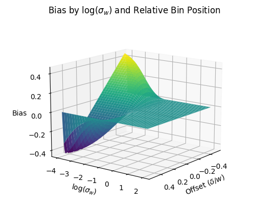
We used simulation to approximate the bias as a function of $\sigma$ and padding. We did this by generating simulated data, transforming it to a discretized truncated Gaussian distribution, and comparing the mean of this distribution to the original value. We first attempted to isolate the discretization bias by computing the total bias and using large padding, since the truncation bias vanishes as the support for the distribution grows to $(-\infty,\infty)$. By generating $10^{5}$ equally spaced data points in the range $[0,1]$ divided into $k=100$ bins of equal width and varying $\sigma$ we can plot the discretization bias as a function of $\sigma_{w}$, defined as $\sigma/(1/k)$, and the relative position within a bin. We used padding of $\psi=100$. Define $\psi_{\sigma}$ as $\psi/\sigma$. The bin width is then adjusted as in the following equation:

$$w=\frac{y_{max}-y_{min}}{k-2\sigma_{w}\psi_{\sigma}}$$ (16)

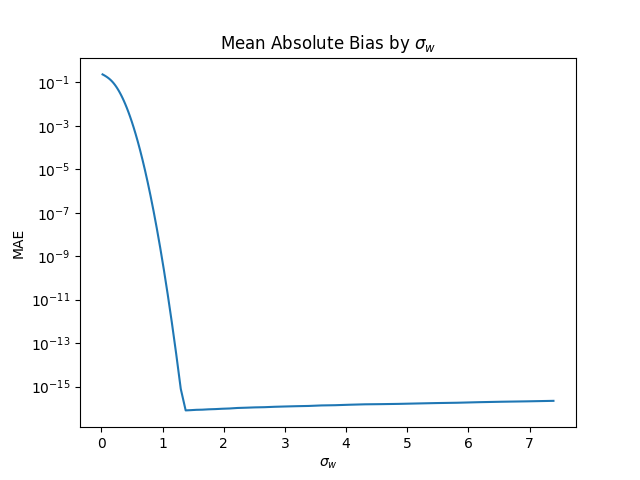
Figure 11 (left) displays the results. We define $\delta$ as the difference between the sample and the center of the bin and the offset as $\frac{\delta}{w}$. The X-axis ($\sigma_{w}$) has been log-transformed. As expected by the symmetry of the Gaussian distribution, we have zero bias for the center of the bin. The relationship with the bin offset converges to linear as $\sigma_{w}\to 0$, which corresponds to convergence towards HL-Onebin. The error also decreases to zero as $\sigma_{w}\to\infty$. Taking the mean absolute bias over all samples, we obtain Figure 11 (middle). Due to the log scale of the Y-axis, the approximate parabolic decrease in error is actually a squared-exponential decay. The graph reaches a minimum at around $\sigma_{w}\approx 1.35$ before increasing slowly, as the bias is dominated by 64-bit floating point precision error.

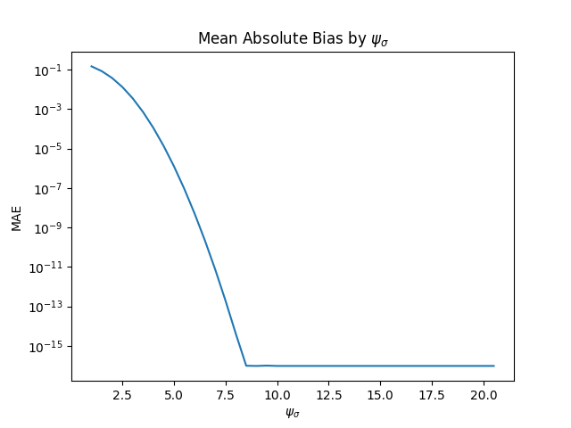
We can also observe the total error for different values of $\psi_{\sigma}$ in Figure 11 (right). Fixing $\sigma_{w}=2$, the discretization error is negligible. Again, we see squared-exponential decay as the padding increases until $\psi_{\sigma}=8.5$, after which the bias is dominated by floating point precision error. Overall, for $\sigma_{w}>0.8$ and $\psi_{\sigma}>6$, we have bias less than $10^{-7}$ which is negligible when using 32-bit floating point numbers. Empirically, the effect of these parameters on model learning has a greater impact on performance, but these graphs can be used to approximate the bias after scaling by the bin width.

Figure 11: Bias simulation results. (Left) Discretization bias, (Middle) Mean Absolute Discretization Bias, (Right) Mean Absolute Truncation Bias.

C Empirical Study - Details

C.1 Dataset details

Table 6 and Figure 12 show the details of the four regression datasets.

Dataset	# train	# test	# feats	$Y$ range
Song Year	412276	103069	90	[1922,2011]
CT Position	42800	10700	385	[0,100]
Bike Sharing	13911	3478	16	[0,1000]
Pole	12000	3000	49	[0,100]

Table 6: Overview of the datasets used in the experiments.

Figure 12: Histograms of the target values for the four datasets. Each plot shows a histogram with 30 bins, where the area of a bin is the ratio of targets in the dataset that fall in that bin. Note that it is the total area of bins, and not the sum of heights, that equals one.

C.2 Architectures and Hyperparameters

The architecture for CT Position is 385-192-192-192-192-1, for Song Year is 90-45-45-45-45-1 (4 hidden layers of size 45), for Bike Sharing is 16-64-64-64-64-1, and for Pole is 49-24-24-24-1. All hidden layers employ ReLU activation. Network architectures were chosen according to best Test MAE for $\ell_{2}$, with depth and width varied across 7 different values.

Some of the baselines required extra hyperparameters. The range of these hyperparameters are described below:
$\mathbf{\ell_{2}}$+Noise The standard deviation of the noise is selected from $\{10^{-5},10^{-4},10^{-3},10^{-2},10^{-1}\}$.
$\mathbf{\ell_{2}}$+Clipping The threshold for clipping is selected from $\{0.01,0.1,1,10\}$.
HL-Uniform $\epsilon\in\{10^{-5},10^{-4},10^{-3},10^{-2},10^{-1}\}$.
MDN The originally proposed model uses an exponential activation to model the standard deviations. However, inspired by Lakshminarayanan et al. (2017), we used softplus activation plus a small constant ($10^{-2}$) to avoid numerical instability. We selected the number of components from $\{2,4,8,16,32\}$. Predictions are made by taking the mean of the mixture model given by the MDN.

We used Scikit-learn (Pedregosa et al., 2011) for the implementations of Linear Regression, and Keras (Chollet et al., 2015) for the neural network models. All neural network models are trained with mini-batch size 256 using the Adam optimizer (Kingma and Ba, 2015) with a learning rate 1e-3 and the parameters are initialized according to the method suggested by LeCun et al. (1998). Dropout (Srivastava et al., 2014) with rate $0.05$ is added to the input layer of all neural networks for CT Scan and Song Year tasks to avoid overfitting. We trained the networks for 1000 epochs on CT Position, 150 epochs on Song Year and 500 epochs on Bike Sharing and Pole. Dropout is disabled in the experiments in Section 4.7.

D Application - Details

D.1 Time Series Prediction

The linear model uses a single fully connected layer to predict the prediction target as a linear function of input timesteps, as suggested by Zeng et al. (2023). We used a vanilla-transformer architecture (Vaswani et al., 2017) with $3$ self-attention blocks, $3$ heads each of size $256$. For LSTM, we used a single-layer LSTM with $256$ hidden units.

We did a train-test split of $12$-$4$ months ($30$ days per month). In all the experiments, the input sequences had a length of $336$, and the prediction target was $96$ steps ahead into the future. We trained all networks for $25$ epochs with a batch size of $32$ using ADAM optimizer with learning rate $\alpha=10^{-4}$, $\beta_{1}=0.9$, $\beta_{2}=0.999$, and $\epsilon=10^{-7}$. We standardized the data using the mean and standard deviation of the data. All models were implemented using Keras (Chollet et al. (2015)).

For the HL-Gaussian model, the bin width was determined as in Equation (16) where $\sigma_{w}$ is the ratio of the $\sigma$ parameter for the truncated Gaussian distribution to the bin width, and $\psi_{\sigma}$ is the ratio of padding to bin width added to each side. We used $k=100$ bins with $\sigma_{w}=2$ and $\psi_{\sigma}=3$. The bin widths are calculated independently for each variable using the corresponding minimum and maximum observation over the entire dataset.

D.2 Value Prediction

We first precomputed the values for each game. Then, we trained on the first 95% of the game iterations in the actions file and tested on the remaining 5% of the iterations. The samples were shuffled with a buffer size of 1000 within the training and testing sets. We scaled the targets to be in the range $[0,1]$. The model backbone consists of 3 convolutional layers followed by a fully-connected layer. We used an ADAM optimizer with parameters $\alpha=0.001$, $\beta_{1}=0.9$, $\beta_{2}=0.999$, and $\epsilon=10^{-7}$. All models were implemented using Keras (Chollet et al. (2015)).

For HL-Gaussian We used $k=100$ bins with $\sigma_{w}=2$ and $\psi_{\sigma}=4$ in Equation (16). The models were trained for 1-3 epochs, depending on the game.

E Other Results

This section provides the rest of the empirical results.

E.1 Overall Results

Method	Train MAE	Train RMSE	Test MAE	Test RMSE
Lin Reg	$6.793$$(\pm 0.003)$	$9.547$$(\pm 0.003)$	$6.796$$(\pm 0.007)$	$9.555$$(\pm 0.014)$
$\ell_{2}$	$5.758$$(\pm 0.026)$	$8.137$$(\pm 0.014)$	$6.016$$(\pm 0.022)$	$8.690$$(\pm 0.015)$
$\ell_{2}$+Noise	$5.697$$(\pm 0.023)$	$8.124$$(\pm 0.006)$	$5.959$$(\pm 0.015)$	$8.682$$(\pm 0.022)$
$\ell_{2}$+Clip	$5.749$$(\pm 0.032)$	$8.130$$(\pm 0.012)$	$6.009$$(\pm 0.032)$	$8.687$$(\pm 0.015)$
$\ell_{1}$	$5.423$$(\pm 0.010)$	$8.640$$(\pm 0.016)$	$5.673$$(\pm 0.006)$	$8.987$$(\pm 0.025)$
MDN	$5.858$$(\pm 0.020)$	$8.530$$(\pm 0.008)$	$5.935$$(\pm 0.025)$	$8.640$$(\pm 0.020)$
$\ell_{2}$+softmax	$5.651$$(\pm 0.015)$	$8.067$$(\pm 0.009)$	$5.947$$(\pm 0.012)$	$8.685$$(\pm 0.012)$
HL-OneBin	$5.810$$(\pm 0.010)$	$8.487$$(\pm 0.002)$	$5.906$$(\pm 0.020)$	$8.636$$(\pm 0.020)$
HL-Gauss.	$5.789$$(\pm 0.004)$	$8.440$$(\pm 0.004)$	$5.903$$(\pm 0.010)$	$8.621$$(\pm 0.016)$

Method	Train MAE	Train RMSE	Test MAE	Test RMSE
Lin Reg	$106.047$$(\pm 0.215)$	$141.854$$(\pm 0.192)$	$105.788$$(\pm 0.738)$	$141.617$$(\pm 0.757)$
$\ell_{2}$	$14.453$$(\pm 0.258)$	$19.487$$(\pm 0.116)$	$31.029$$(\pm 0.258)$	$48.205$$(\pm 0.545)$
$\ell_{2}$+Noise	$20.577$$(\pm 0.270)$	$28.604$$(\pm 0.325)$	$28.486$$(\pm 0.278)$	$44.777$$(\pm 0.747)$
$\ell_{2}$+Clip	$13.221$$(\pm 0.676)$	$18.011$$(\pm 0.783)$	$29.404$$(\pm 0.188)$	$46.309$$(\pm 0.403)$
$\ell_{1}$	$12.764$$(\pm 0.250)$	$21.456$$(\pm 0.356)$	$27.550$$(\pm 0.258)$	$44.717$$(\pm 0.674)$
MDN	$15.406$$(\pm 0.192)$	$27.593$$(\pm 0.348)$	$26.268$$(\pm 0.342)$	$43.679$$(\pm 0.605)$
$\ell_{2}$+softmax	$11.991$$(\pm 0.277)$	$16.799$$(\pm 0.445)$	$27.827$$(\pm 0.253)$	$45.825$$(\pm 0.431)$
HL-OneBin	$15.822$$(\pm 0.198)$	$26.065$$(\pm 0.335)$	$26.689$$(\pm 0.280)$	$45.150$$(\pm 0.857)$
HL-Gauss.	$14.335$$(\pm 0.152)$	$23.178$$(\pm 0.309)$	$25.525$$(\pm 0.331)$	$43.671$$(\pm 0.796)$

Method	Train MAE	Train RMSE	Test MAE	Test RMSE
Lin Reg	$26.523$$(\pm 0.018)$	$30.424$$(\pm 0.010)$	$26.662$$(\pm 0.066)$	$30.567$$(\pm 0.038)$
$\ell_{2}$	$0.767$$(\pm 0.016)$	$1.441$$(\pm 0.026)$	$1.131$$(\pm 0.024)$	$2.579$$(\pm 0.073)$
$\ell_{2}$+Noise	$0.700$$(\pm 0.031)$	$1.406$$(\pm 0.039)$	$1.062$$(\pm 0.027)$	$2.529$$(\pm 0.054)$
$\ell_{2}$+Clip	$0.714$$(\pm 0.018)$	$1.424$$(\pm 0.024)$	$1.069$$(\pm 0.017)$	$2.551$$(\pm 0.103)$
$\ell_{1}$	$0.637$$(\pm 0.013)$	$1.661$$(\pm 0.029)$	$0.938$$(\pm 0.029)$	$2.584$$(\pm 0.034)$
MDN	$0.648$$(\pm 0.026)$	$1.712$$(\pm 0.078)$	$0.895$$(\pm 0.013)$	$2.480$$(\pm 0.095)$
$\ell_{2}$+softmax	$0.634$$(\pm 0.017)$	$1.445$$(\pm 0.019)$	$0.950$$(\pm 0.016)$	$2.481$$(\pm 0.055)$
HL-OneBin	$0.899$$(\pm 0.015)$	$1.442$$(\pm 0.033)$	$1.264$$(\pm 0.019)$	$2.760$$(\pm 0.116)$
HL-Gauss.	$0.347$$(\pm 0.018)$	$1.299$$(\pm 0.049)$	$0.714$$(\pm 0.024)$	$2.673$$(\pm 0.141)$

Table 7: Overall results on the other datasets. The tables show Song Year, Bike Sharing, and Pole from top to bottom. Song Year: $\ell_{1}$ outperformed HL-Gaussian in terms of Test MAE, there was not a substantial difference between the performance of HL-OneBin and HL-Gaussian, and the rest of the methods had higher error rates than HL-Gaussian. The differences in error rates were small on this dataset and even Linear Regression worked well. Bike Sharing: HL-Gaussian had the lowest Test MAE on this dataset and $\ell_{2}$ performed the worst among neural network methods. Pole: HL-Gaussian achieved the lowest Test MAE. The other methods did not achieve a Test MAE close to that of HL-Gaussian, and there was a noticeable gap between the performance of HL-OneBin and HL-Gaussian.

Figure 13: HL-Uniform results. The rows show CT Scan, Song Year, Bike, and Pole respectively. Dotted and solid lines show train and test errors respectively. The parameter $\epsilon$ is the weighting on the uniform distribution and raising it only impaired performance.

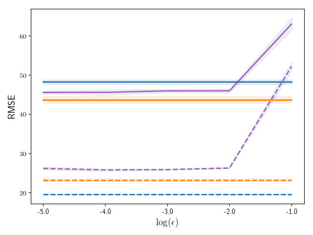
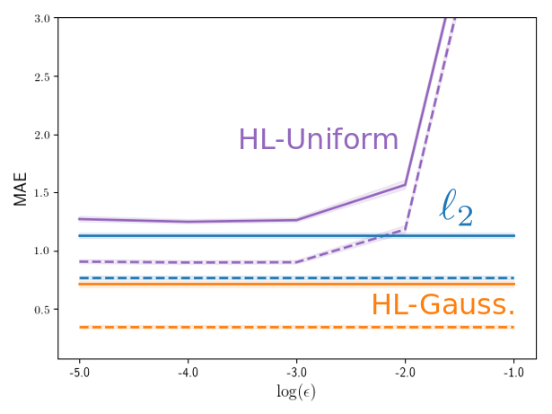
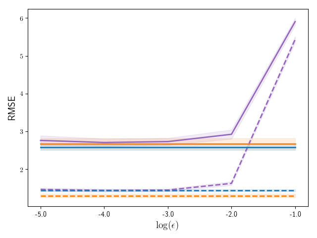
E.2 Bias and the Choice of Target Distribution

Method	Train MAE	Train RMSE	Test MAE	Test RMSE
HL-OneBin	$0.309$$(\pm 0.000)$	$0.364$$(\pm 0.006)$	$0.335$$(\pm 0.004)$	$0.660$$(\pm 0.099)$
HL-Projected	$0.053$$(\pm 0.001)$	$0.074$$(\pm 0.002)$	$0.103$$(\pm 0.003)$	$0.462$$(\pm 0.065)$
HL-Gauss.	$0.061$$(\pm 0.006)$	$0.164$$(\pm 0.090)$	$0.098$$(\pm 0.005)$	$0.274$$(\pm 0.090)$

Method	Train MAE	Train RMSE	Test MAE	Test RMSE
HL-OneBin	$5.810$$(\pm 0.010)$	$8.487$$(\pm 0.002)$	$5.906$$(\pm 0.020)$	$8.636$$(\pm 0.020)$
HL-Projected	$5.815$$(\pm 0.012)$	$8.477$$(\pm 0.003)$	$5.917$$(\pm 0.019)$	$8.629$$(\pm 0.016)$
HL-Gauss.	$5.789$$(\pm 0.004)$	$8.440$$(\pm 0.004)$	$5.903$$(\pm 0.010)$	$8.621$$(\pm 0.016)$

Method	Train MAE	Train RMSE	Test MAE	Test RMSE
HL-OneBin	$15.822$$(\pm 0.198)$	$26.065$$(\pm 0.335)$	$26.689$$(\pm 0.280)$	$45.150$$(\pm 0.857)$
HL-Projected	$14.885$$(\pm 0.169)$	$24.329$$(\pm 0.329)$	$26.180$$(\pm 0.348)$	$44.982$$(\pm 0.845)$
HL-Gauss.	$14.335$$(\pm 0.152)$	$23.178$$(\pm 0.309)$	$25.525$$(\pm 0.331)$	$43.671$$(\pm 0.796)$

Method	Train MAE	Train RMSE	Test MAE	Test RMSE
HL-OneBin	$0.899$$(\pm 0.015)$	$1.442$$(\pm 0.033)$	$1.264$$(\pm 0.019)$	$2.760$$(\pm 0.116)$
HL-Projected	$0.364$$(\pm 0.020)$	$1.340$$(\pm 0.055)$	$0.741$$(\pm 0.018)$	$2.753$$(\pm 0.068)$
HL-Gauss.	$0.347$$(\pm 0.018)$	$1.299$$(\pm 0.049)$	$0.714$$(\pm 0.024)$	$2.673$$(\pm 0.141)$

Table 8: Discretization bias experiment. The tables show CT-Scan, Song Year, Bike Sharing, and Pole from top to bottom. Overall, HL-Projected achieved a Test MAE close to that of HL-Gaussian, and performed noticeably better than HL-OneBin.

Figure 14: MAE between the means of HL targets and the original labels. It can be seen that extreme values of $\sigma$ on either side biased the mean of the target distributions.

Figure 15: Changing the number of bins. The rows show CT Scan, Song Year, Bike Sharing, and Pole respectively. Dotted and solid lines show train and test errors respectively. A small number of bins resulted in high train and test errors, indicating high bias. A higher number of bins generally did not result in a rise in test error, with the exception of HL-OneBin’s test RMSE on CT Scan.

Figure 16: Changing the parameter $\sigma$. The rows show CT Scan, Song Year, Bike Sharing, and Pole respectively. Dotted and solid lines show train and test errors respectively. Generally, extreme values of $\sigma$, especially to the right, resulted in bad performance. The error rates for train and test followed each other when changing this parameter.

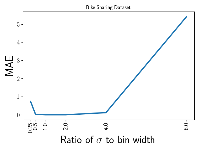
E.3 Representation

	Loss	Default	Fixed	Initialized	Random
Train MAE	$\ell_{2}$	$5.758$$(\pm 0.026)$	$6.268$$(\pm 0.055)$	$5.743$$(\pm 0.015)$	$8.060$$(\pm 0.024)$
Train MAE	HL-Gauss.	$5.789$$(\pm 0.004)$	$5.682$$(\pm 0.014)$	$5.781$$(\pm 0.010)$	$7.942$$(\pm 0.021)$
Train RMSE	$\ell_{2}$	$8.137$$(\pm 0.014)$	$8.797$$(\pm 0.030)$	$8.131$$(\pm 0.003)$	$10.730$$(\pm 0.016)$
Train RMSE	HL-Gauss.	$8.440$$(\pm 0.004)$	$8.130$$(\pm 0.010)$	$8.396$$(\pm 0.007)$	$10.691$$(\pm 0.026)$
Test MAE	$\ell_{2}$	$6.016$$(\pm 0.022)$	$6.338$$(\pm 0.063)$	$5.997$$(\pm 0.028)$	$8.069$$(\pm 0.029)$
Test MAE	HL-Gauss.	$5.903$$(\pm 0.010)$	$5.954$$(\pm 0.011)$	$5.900$$(\pm 0.016)$	$7.952$$(\pm 0.017)$
Test RMSE	$\ell_{2}$	$8.690$$(\pm 0.015)$	$8.901$$(\pm 0.046)$	$8.666$$(\pm 0.021)$	$10.748$$(\pm 0.014)$
Test RMSE	HL-Gauss.	$8.621$$(\pm 0.016)$	$8.723$$(\pm 0.013)$	$8.603$$(\pm 0.013)$	$10.712$$(\pm 0.010)$

	Loss	Default	Fixed	Initialized	Random
Train MAE	$\ell_{2}$	$14.453$$(\pm 0.258)$	$39.101$$(\pm 1.054)$	$18.214$$(\pm 1.154)$	$106.376$$(\pm 0.569)$
Train MAE	HL-Gauss.	$14.335$$(\pm 0.152)$	$30.171$$(\pm 0.469)$	$12.571$$(\pm 0.250)$	$99.251$$(\pm 1.069)$
Train RMSE	$\ell_{2}$	$19.487$$(\pm 0.116)$	$53.545$$(\pm 1.264)$	$23.833$$(\pm 1.137)$	$142.523$$(\pm 1.052)$
Train RMSE	HL-Gauss.	$23.178$$(\pm 0.309)$	$42.140$$(\pm 0.664)$	$20.320$$(\pm 0.518)$	$136.065$$(\pm 1.283)$
Test MAE	$\ell_{2}$	$31.029$$(\pm 0.258)$	$42.834$$(\pm 0.983)$	$31.119$$(\pm 0.906)$	$106.429$$(\pm 0.982)$
Test MAE	HL-Gauss.	$25.525$$(\pm 0.331)$	$37.696$$(\pm 0.360)$	$25.470$$(\pm 0.202)$	$99.311$$(\pm 1.486)$
Test RMSE	$\ell_{2}$	$48.205$$(\pm 0.545)$	$59.890$$(\pm 0.674)$	$46.735$$(\pm 0.387)$	$143.052$$(\pm 1.472)$
Test RMSE	HL-Gauss.	$43.671$$(\pm 0.796)$	$56.350$$(\pm 0.525)$	$43.809$$(\pm 0.593)$	$136.941$$(\pm 1.639)$

	Loss	Default	Fixed	Initialized	Random
Train MAE	$\ell_{2}$	$0.767$$(\pm 0.016)$	$4.218$$(\pm 0.325)$	$1.109$$(\pm 0.024)$	$28.936$$(\pm 0.176)$
Train MAE	HL-Gauss.	$0.347$$(\pm 0.018)$	$1.218$$(\pm 0.052)$	$0.312$$(\pm 0.010)$	$18.428$$(\pm 0.969)$
Train RMSE	$\ell_{2}$	$1.441$$(\pm 0.026)$	$6.184$$(\pm 0.412)$	$1.836$$(\pm 0.042)$	$33.642$$(\pm 0.231)$
Train RMSE	HL-Gauss.	$1.299$$(\pm 0.049)$	$2.899$$(\pm 0.143)$	$1.212$$(\pm 0.027)$	$26.795$$(\pm 0.959)$
Test MAE	$\ell_{2}$	$1.131$$(\pm 0.024)$	$4.396$$(\pm 0.329)$	$1.437$$(\pm 0.053)$	$29.221$$(\pm 0.254)$
Test MAE	HL-Gauss.	$0.714$$(\pm 0.024)$	$1.398$$(\pm 0.021)$	$0.645$$(\pm 0.009)$	$18.285$$(\pm 1.062)$
Test RMSE	$\ell_{2}$	$2.579$$(\pm 0.073)$	$6.423$$(\pm 0.415)$	$2.882$$(\pm 0.109)$	$33.944$$(\pm 0.299)$
Test RMSE	HL-Gauss.	$2.673$$(\pm 0.141)$	$3.441$$(\pm 0.093)$	$2.373$$(\pm 0.055)$	$26.621$$(\pm 1.043)$

Table 9: Representation results on the other datasets. The tables show Song Year, Bike Sharing, and Pole from top to bottom. We tested (a) swapping the representations and re-learning on the last layer (Fixed), (b) initializing with the other’s representation (Initialized), (c) and using the same fixed random representation for both (Random) and only learning the last layer. In general, $\ell_{2}$ underperformed HL-Gaussian in all the three settings. Using HL-Gaussian’s fixed representation only made the performance of $\ell_{2}$ worse. As an initialization, it did not result in a considerable improvement.

Figure 17: Multi-Task Network results. The rows show CT Scan, Song Year, Bike Sharing, and Pole respectively. The loss function is the mean prediction’s squared error plus the distribution prediction’s KL-divergence multiplied by a coefficient. The horizontal axis shows the coefficient for KL-divergence. Dotted and solid lines show train and test errors respectively. There was not a substantial drop in the error rate when increasing the coefficient in the loss and the performance only became worse.

Figure 18: Higher Moments Network results. The rows show CT Scan, Song Year, Bike Sharing, and Pole respectively. The X-axis shows the number of moments (including the mean). Dotted and solid lines show train and test errors respectively. There was no substantial decrease in error when predicting higher moments. In some cases there was a slight reduction in error but the new model still performed worse than HL-Gaussian in terms of Test MAE.

E.4 Optimization Properties

Figure 19: Training process. The rows show CT Scan, Song Year, Bike Sharing, and Pole respectively. A logarithmic scale is used in the Y axis of the rightmost plot. In all cases, training with HL-Gaussian resulted in initial fast reduction in train MAE compared to $\ell_{2}$. The gradient norm of $\ell_{2}$ was highly varying through the training.

Figure 20: Annealing results. The rows show Ct Scan, Song Year, Bike Sharing, and Pole respectively. Dotted and solid lines show train and test errors. On three datasets, there was a small benefit in starting with a higher $\sigma$ and reducing it though the training.

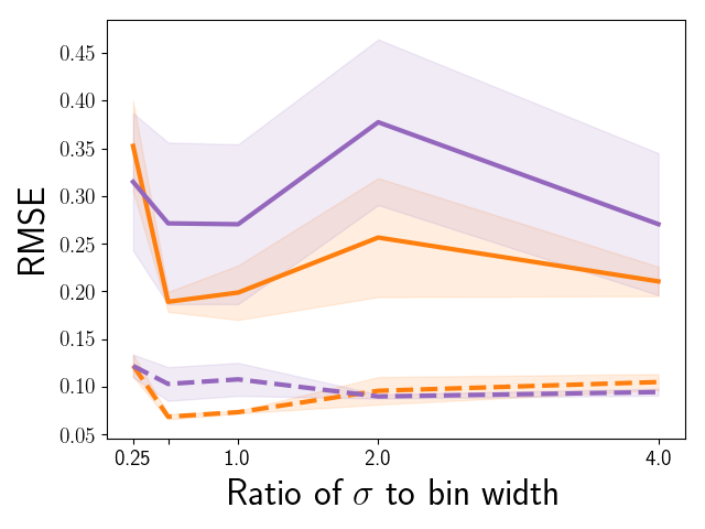
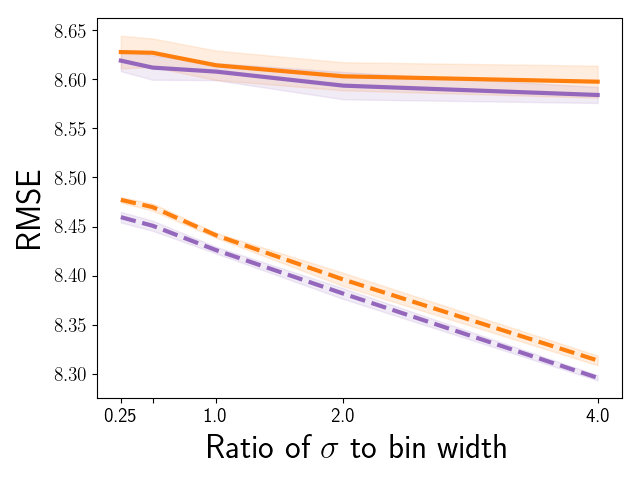
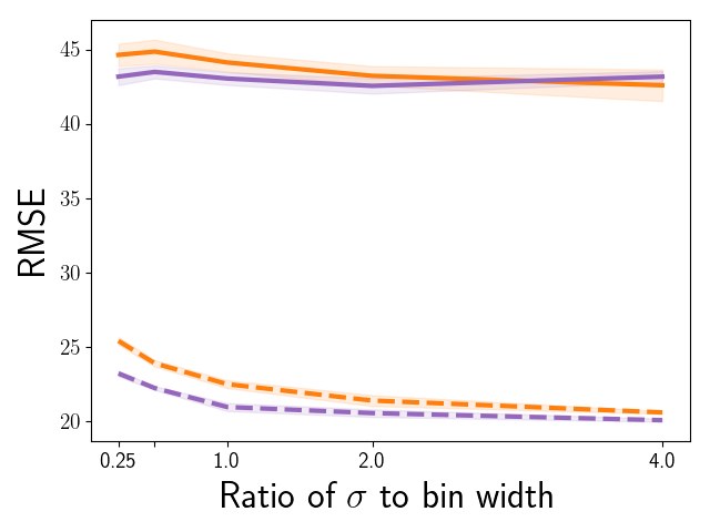
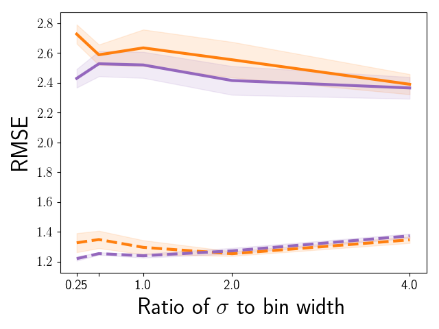
F Robustness to Corrupted Targets

Figure 21: Corrupted targets results. The rows show CT Scan, Song Year, Bike Sharing, and Pole respectively. The lines show test errors. The $\ell_{1}$ loss was robust to corrupted targets, and the $\ell_{2}$ loss was affected the most.

G Sensitivity to Input Perturbations

Figure 22: Sensitivity results. The rows show CT Scan, Song Year, Bike Sharing, and Pole respectively. The horizontal axis shows the sensitivity of the model’s output to input perturbations (left means less sensitive) and the vertical axis shows the test error (lower is better). HL-Gaussian showed less sensitivity and lower test errors than $\ell_{1}$ and $\ell_{2}$.

References

- Arora et al. (2018) Sanjeev Arora, Nadav Cohen, and Elad Hazan. On the optimization of deep networks: Implicit acceleration by overparameterization. In International Conference on Machine Learning, 2018.
- Barron (2019) Jonathan T Barron. A general and adaptive robust loss function. In IEEE Conference on Computer Vision and Pattern Recognition, 2019.
- Bellemare et al. (2013) M. G. Bellemare, Y. Naddaf, J. Veness, and M. Bowling. The arcade learning environment: An evaluation platform for general agents. Journal of Artificial Intelligence Research, 2013.
- Bellemare et al. (2017) Marc G Bellemare, Will Dabney, and Rémi Munos. A distributional perspective on reinforcement learning. In International Conference on Machine Learning, 2017.
- Bellemare et al. (2023) Marc G Bellemare, Will Dabney, and Mark Rowland. Distributional reinforcement learning. 2023.
- Bertin-Mahieux et al. (2011) Thierry Bertin-Mahieux, Daniel PW Ellis, Brian Whitman, and Paul Lamere. The million song dataset. In Ismir, 2011.
- Bishop (2006) C Bishop. Pattern recognition and machine learning. 2006.
- Bishop (1994) Christopher M Bishop. Mixture density networks. Technical Report, 1994.
- Canonne (2022) Clément L Canonne. A short note on an inequality between kl and tv. arXiv, 2022.
- Charbonnier et al. (1994) Pierre Charbonnier, Laure Blanc-Feraud, Gilles Aubert, and Michel Barlaud. Two deterministic half-quadratic regularization algorithms for computed imaging. In International Conference on Image Processing, 1994.
- Chollet et al. (2015) François Chollet et al. Keras, 2015.
- Choromanska et al. (2015) Anna Choromanska, Mikael Henaff, Michael Mathieu, Gérard Ben Arous, and Yann LeCun. The loss surfaces of multilayer networks. In Artificial Intelligence and Statistics, 2015.
- Dabney et al. (2018a) Will Dabney, Georg Ostrovski, David Silver, and Rémi Munos. Implicit quantile networks for distributional reinforcement learning. In International conference on machine learning, 2018a.
- Dabney et al. (2018b) Will Dabney, Mark Rowland, Marc Bellemare, and Rémi Munos. Distributional reinforcement learning with quantile regression. In AAAI Conference on Artificial Intelligence, 2018b.
- Dinh et al. (2017) Laurent Dinh, Razvan Pascanu, Samy Bengio, and Yoshua Bengio. Sharp minima can generalize for deep nets. In International Conference on Machine Learning, 2017.
- Fanaee-T and Gama (2014) Hadi Fanaee-T and Joao Gama. Event labeling combining ensemble detectors and background knowledge. Progress in Artificial Intelligence, 2014.
- Foret et al. (2021) Pierre Foret, Ariel Kleiner, Hossein Mobahi, and Behnam Neyshabur. Sharpness-aware minimization for efficiently improving generalization. In International Conference on Learning Representations, 2021.
- Fujita et al. (2021) Yasuhiro Fujita, Prabhat Nagarajan, Toshiki Kataoka, and Takahiro Ishikawa. Chainerrl: A deep reinforcement learning library. Journal of Machine Learning Research, 2021.
- Gao et al. (2017) Bin-Bin Gao, Chao Xing, Chen-Wei Xie, Jianxin Wu, and Xin Geng. Deep label distribution learning with label ambiguity. IEEE Transactions on Image Processing, 2017.
- Graf et al. (2011) Franz Graf, Hans-Peter Kriegel, Matthias Schubert, Sebastian Pölsterl, and Alexander Cavallaro. 2d image registration in ct images using radial image descriptors. Medical Image Computing and Computer-Assisted Intervention, 2011.
- Hardt et al. (2016) Moritz Hardt, Ben Recht, and Yoram Singer. Train faster, generalize better: Stability of stochastic gradient descent. In International Conference on Machine Learning, 2016.
- Hessel et al. (2018) Matteo Hessel, Joseph Modayil, Hado Van Hasselt, Tom Schaul, Georg Ostrovski, Will Dabney, Dan Horgan, Bilal Piot, Mohammad Azar, and David Silver. Rainbow: Combining improvements in deep reinforcement learning. In AAAI conference on artificial intelligence, 2018.
- Hochreiter and Schmidhuber (1997a) Sepp Hochreiter and Jürgen Schmidhuber. Flat minima. Neural computation, 1997a.
- Hochreiter and Schmidhuber (1997b) Sepp Hochreiter and Jürgen Schmidhuber. Long short-term memory. Neural computation, 1997b.
- Hoffer et al. (2017) Elad Hoffer, Itay Hubara, and Daniel Soudry. Train longer, generalize better: closing the generalization gap in large batch training of neural networks. Advances in neural information processing systems, 2017.
- Huber (2011) Peter J Huber. Robust statistics. In International Encyclopedia of Statistical Science. 2011.
- Imani and White (2018) Ehsan Imani and Martha White. Improving regression performance with distributional losses. In International Conference on Machine Learning, 2018.
- Jacot et al. (2018) Arthur Jacot, Franck Gabriel, and Clément Hongler. Neural tangent kernel: Convergence and generalization in neural networks. Advances in Neural Information Processing Systems, 2018.
- Javed et al. (2023) Khurram Javed, Haseeb Shah, Richard S. Sutton, and Martha White. Scalable real-time recurrent learning using columnar-constructive networks. Journal of Machine Learning Research, 2023.
- Jiang et al. (2020) Yiding Jiang, Behnam Neyshabur, Hossein Mobahi, Dilip Krishnan, and Samy Bengio. Fantastic generalization measures and where to find them. In International Conference on Learning Representations, 2020.
- Keskar et al. (2017) Nitish Shirish Keskar, Dheevatsa Mudigere, Jorge Nocedal, Mikhail Smelyanskiy, and Ping Tak Peter Tang. On large-batch training for deep learning: Generalization gap and sharp minima. In International Conference on Learning Representations, 2017.
- Kingma and Ba (2015) Diederik Kingma and Jimmy Ba. Adam: A method for stochastic optimization. In International Conference on Learning Representations, 2015.
- Lakshminarayanan et al. (2017) Balaji Lakshminarayanan, Alexander Pritzel, and Charles Blundell. Simple and scalable predictive uncertainty estimation using deep ensembles. In Advances in Neural Information Processing Systems, 2017.
- Lan et al. (2022) Charline Le Lan, Stephen Tu, Adam Oberman, Rishabh Agarwal, and Marc G Bellemare. On the generalization of representations in reinforcement learning. In International Conference on Artificial Intelligence and Statistics, 2022.
- Lattimore and Szepesvári (2020) Tor Lattimore and Csaba Szepesvári. Bandit algorithms. Cambridge University Press, 2020.
- LeCun et al. (1998) Yann LeCun, Léon Bottou, Genevieve B Orr, and Klaus-Robert Müller. Efficient backprop. In Neural networks: Tricks of the trade. 1998.
- Li et al. (2018) Hao Li, Zheng Xu, Gavin Taylor, Christoph Studer, and Tom Goldstein. Visualizing the loss landscape of neural nets. In Advances in Neural Information Processing Systems, 2018.
- Lyle et al. (2019) Clare Lyle, Marc G Bellemare, and Pablo Samuel Castro. A comparative analysis of expected and distributional reinforcement learning. In AAAI Conference on Artificial Intelligence, 2019.
- Lyle et al. (2021) Clare Lyle, Mark Rowland, Georg Ostrovski, and Will Dabney. On the effect of auxiliary tasks on representation dynamics. In International Conference on Artificial Intelligence and Statistics, 2021.
- Norouzi et al. (2016) Mohammad Norouzi, Samy Bengio, Navdeep Jaitly, Mike Schuster, Yonghui Wu, Dale Schuurmans, et al. Reward augmented maximum likelihood for neural structured prediction. In Advances In Neural Information Processing Systems, 2016.
- Novak et al. (2018) Roman Novak, Yasaman Bahri, Daniel A Abolafia, Jeffrey Pennington, and Jascha Sohl-Dickstein. Sensitivity and generalization in neural networks: an empirical study. In International Conference on Learning Representations, 2018.
- Olson et al. (2017) Randal S. Olson, William La Cava, Patryk Orzechowski, Ryan J. Urbanowicz, and Jason H. Moore. Pmlb: a large benchmark suite for machine learning evaluation and comparison. BioData Mining, 2017.
- Pedregosa et al. (2011) F. Pedregosa, G. Varoquaux, A. Gramfort, V. Michel, B. Thirion, O. Grisel, M. Blondel, P. Prettenhofer, R. Weiss, V. Dubourg, J. Vanderplas, A. Passos, D. Cournapeau, M. Brucher, M. Perrot, and E. Duchesnay. Scikit-learn: Machine learning in Python. Journal of Machine Learning Research, 2011.
- Reading et al. (2021) Cody Reading, Ali Harakeh, Julia Chae, and Steven L Waslander. Categorical depth distribution network for monocular 3d object detection. In Conference on Computer Vision and Pattern Recognition, 2021.
- Rifai et al. (2011) Salah Rifai, Pascal Vincent, Xavier Muller, Xavier Glorot, and Yoshua Bengio. Contractive auto-encoders: Explicit invariance during feature extraction. In International Conference on Machine Learning, 2011.
- Rothe et al. (2015) Rasmus Rothe, Radu Timofte, and Luc Van Gool. Dex: Deep expectation of apparent age from a single image. In IEEE International Conference on Computer Vision Workshops, 2015.
- Rowland et al. (2018) Mark Rowland, Marc Bellemare, Will Dabney, Rémi Munos, and Yee Whye Teh. An analysis of categorical distributional reinforcement learning. In International Conference on Artificial Intelligence and Statistics, 2018.
- Sokolić et al. (2017) Jure Sokolić, Raja Giryes, Guillermo Sapiro, and Miguel RD Rodrigues. Robust large margin deep neural networks. IEEE Transactions on Signal Processing, 2017.
- Soltanolkotabi et al. (2018) Mahdi Soltanolkotabi, Adel Javanmard, and Jason D Lee. Theoretical insights into the optimization landscape of over-parameterized shallow neural networks. IEEE Transactions on Information Theory, 2018.
- Srivastava et al. (2014) Nitish Srivastava, Geoffrey Hinton, Alex Krizhevsky, Ilya Sutskever, and Ruslan Salakhutdinov. Dropout: A simple way to prevent neural networks from overfitting. The Journal of Machine Learning Research, 2014.
- Vaswani et al. (2017) Ashish Vaswani, Noam Shazeer, Niki Parmar, Jakob Uszkoreit, Llion Jones, Aidan N Gomez, Łukasz Kaiser, and Illia Polosukhin. Attention is all you need. Advances in neural information processing systems, 2017.
- Zeng et al. (2023) Ailing Zeng, Muxi Chen, Lei Zhang, and Qiang Xu. Are transformers effective for time series forecasting? 2023.
- Zhang (2023) Tong Zhang. Mathematical analysis of machine learning algorithms. Cambridge University Press, 2023.
- Zhou et al. (2021) Haoyi Zhou, Shanghang Zhang, Jieqi Peng, Shuai Zhang, Jianxin Li, Hui Xiong, and Wancai Zhang. Informer: Beyond efficient transformer for long sequence time-series forecasting. In AAAI Conference on Artificial Intelligence, 2021.