An efficient finite element method for computing the response of a strain-limiting elastic solid containing a v-notch and inclusions
Abstract
Accurate triangulation of the domain plays a pivotal role in computing the numerical approximation of the differential operators. A good triangulation is the one which aids in reducing discretization errors. In a standard collocation technique, the smooth curved domain is typically triangulated with a mesh by taking points on the boundary to approximate them by polygons. However, such an approach often leads to geometrical errors which directly affect the accuracy of the numerical approximation. To restrict such geometrical errors, isoparametric, subparametric, and iso-geometric methods were introduced which allow the approximation of the curved surfaces (or curved line segments). In this paper, we present an efficient finite element method to approximate the solution to the elliptic boundary value problem (BVP), which governs the response of an elastic solid containing a v-notch and inclusions. The algebraically nonlinear constitutive equation along with the balance of linear momentum reduces to second-order quasi-linear elliptic partial differential equation. Our approach allows us to represent the complex curved boundaries by smooth one-of-its-kind point transformation. The main idea is to obtain higher-order shape functions which enable us to accurately compute the entries in the finite element matrices and vectors. A Picard-type linearization is utilized to handle the nonlinearities in the governing differential equation. The numerical results for the test cases show considerable improvement in the accuracy.
Keywords— Finite element method; Curved elements; Point transformation; Strain-limiting elastic body; Quasi-linear eliptic partial differential equation.
1 Introduction
The real-world problems are often described by linear or nonlinear partial differential equations posed on complex geometric domains [16, 46]. Simulating such scenarios possesses a lot of challenges arising from nonlinearity in the differential operators [53, 12, 13], geometric complications [52], nonlocality in the boundary conditions [10]. In many instances, the differential operators are approximated by any of the standard collocation methods such as finite difference methods or finite element methods or boundary element methods or spectral methods or even in some cases meshless methods. Creating a good computational mesh for a better approximation in the aforementioned methods is very challenging. In clinical research, the images rendered by computer-aided design software must be accurately represented by meshes (or triangulation). For the finite element computations, the triangulation with straight sides (for example, as in triangles or quadrilaterals) offers a straightforward way of computing the two-dimensional or three-dimensional numerical integrations using high-accurate quadrature rules. This is mainly due to the availability of the standard shape functions (like Lagrange type or any other standard ones) as well as access to the quadrature rules on the regular polygons. Such is not the case when the domain of interest has curved boundaries. The triangulation of such a domain needs to have triangles (or quadrilaterals) with one side curved and the other straight sides to accurately represent the computational domain so that the discretization is minimal (or even zero). The issue is very important when the curved inclusions or heterogeneities are present in the region interesting for computations. Hence, a school of thought of creating curved elements was introduced in [9, 27, 28, 58]. For such curved finite element methods (CFEM), the approximation of the differential operators directly depends on the veracity of the geometrical representation [7, 47]. In CFEM, there are three main approaches: first, the entire global domain containing curved boundary parts is transformed into a standard polygonal shape, and a global computing method can be achieved; second, triangulate the curved region into the regular domain; third, isoparametric finite elements. There are some inherent challenges in these methods [44, 33, 15, 16]. In this paper, we explore the parabolic arcs in matching the curved boundaries (which are the circular inclusions in the domain) by unique point transformations and obtain a higher-order finite element method for cubic order curved triangular element. We explore the numerical technique for approximating the solution of a quasi-linear partial differential equation. The overall algorithm involves Picard’s linearization to handle the nonlinearities and a special finite element method for spatial discretization.
The mathematical model studied in this work governs the response of a limiting-strain elastic solid formulated within the new theory developed in [36, 35, 38, 39, 41, 42, 11, 24, 4, 3, 2]. Such a setup offers an attractive framework to model the response of large class of materials under both mechanical and thermal loading [57, 1]. It is well documented that some materials behave nonlinearly even in less than strain, hence the necessity of developing first-order, yet nonlinear constitutive relations. More importantly, a numerical tool is much needed to correctly approximate the curved regions in the computational domain. Hence, this paper is the first attempt in such a direction.
This paper is organized as follows: In section 2 we introduce the implicit constitutive theory for the response of the elastic solid. A second quasi-linear elliptic partial differential equation is obtained for the anit-plane shear loading setup is also presented in section 2. A BVP and a theorem for the existence of a solution are given in section 3. Section 4 contains a finite element discretization of the BVP. The construction of the shape functions, discrete formulation along with the computational algorithm are all given in the same section. The numerical examples with domains containing v-notch and inclusions are provided in section 5. The conclusions and some information about the future works are given in section 6.
2 Implicit theory of elasticity
In this section, our goal is to provide a brief introduction to an implicit nonlinear theory formulated in a series of papers by Rajagopal [35, 36, 38, 37, 39, 43] for the response of the bulk material. The constitutive relationships are algebraically nonlinear, however, using such relations we develop a mathematical model for the response of an isotropic linear elastic body containing both v-notch and inclusions. The ultimate aim of this investigation is to provide a convergent numerical method for the discretization of the BVP.
Let denote an elastic body that is in equilibrium with the externally applied mechanical loading and we suppose that is the boundary. The elastic material is assumed to occupy a region in two-dimensional space. Let and are the points in the reference and deformed configurations of the body. Let “Sym” be the linear space of symmetric tensors equipped with standard Frobenius norm. We suppose denote the displacement, denote the Cauchy stress, and denotes the infinitesimal strain tensor. The linear space of symmetric tensors equipped with standard Frobenius norm. Let denote the deformation gradient, denote the right Cauchy-Green stretch tensor, denote the left Cauchy-Green stretch tensor, denote the Lagrange strain, respectively defined by:
| (1a) | ||||
| (1b) | ||||
where denotes the transpose operator, is the identity tensor, respectively. The infinitesimal strain theory assumes that
| (2) |
The above assumption (2) implies
| (3) |
Rajagopal [36] generalized the constitutive relationships of Cauchy elasticity by introducing implicit elastic response relations as
| (4) |
where is tensor-valued, the isotropic function such that it obeys [36, 42, 11, 26, 24]
| (5) |
where indicates the orthogonal group. Rajagopal [36] considered a special subclass of (4):
| (6) |
If such a constant exists, then the response relations (6) are referred to as strain-limiting [24, 26]. Applying the standard linearization procedure (2) to (6), we obtain
| (7a) | ||||
| (7b) | ||||
Finally, the governing system of equations to model the behavior of an elastic material within the framework of algebraically nonlinear theories is given by
| (8a) | ||||
| (8b) | ||||
| (8c) | ||||
| (8d) | ||||
Where both and are functions of invariants of the Cauchy stress.
Remark 1.
In the above governing system of equations, equation (8a)1 is from the balance of linear momentum for the quasi-static situation and with the body force acting on the material and equation (8a)2 is from the balance of angular momentum. Equation (8b) is the constitutive relationship governing the response of the material to mechanical/thermal stimuli. Equation (8c) is the strain-compatibility condition and equation (8d) is the equation for the linearized strain.
2.1 Anti-plane Shear Problem (Mode-III)
Our main objective in this work is to provide an efficient method to simulate the response of a strain-limiting elastic body containing v-notch and inclusions and to the authors’ best knowledge, this is the first attempt to investigate a simulation tool for such a setup of algebraically nonlinear constitutive relations. The problem is a static v-notch in a material that is under mode-III loading. In the current loading situation the displacement is a scalar function of and , i.e.
| (9) |
The constitutive relation for the linear, isotropic, and homogeneous material is
| (10) |
where is the shear modulus (N/m2) of the material. Then the constitutive equation within strain-limiting theory of elasticity is
| (11) |
Let us introduce Airy’s stress function and the stress components through the gradient of as
| (12) |
which readily satisfies the balance of linear momentum
| (13) |
The strain-compatibility equation (8c) reduces to the system of equations for the strain components:
| (14a) | ||||
| (14b) | ||||
Notice that the components of the strain tensor depend only on the in-plane coordinates and , we obtain that
| (15) |
From equation (8b), the components of the strain tensor be written as:
| (16) |
Notice that we have used the simpler constitutive relationship with only the second term in (8b). Then using (16) in (15) and also utilizing the Airy’s stress function via the balance of linear momentum (13), we obtain a second-order quasilinear elliptic partial differential equation for
| (17) |
with
| (18) |
For the development of a BVP, we use the following form for :
| (19) |
Remark 2.
It is clear that is both invertible and monotone and generates hyperelastic relations and nonhyperelastic in some cases [23, 22, 43, 37, 40]. It is clear that the monotonically decreasing function satisfies
| (20) |
where depends on the material parameters. An important consequence of (20) is when the “strains” will be uniformly bounded in the entire material body including at the vicinity of concentrators such as crack-tip or re-entrant corner.
Remark 3.
The second-order quasi-linear elliptic partial differential equation derived in this paper is similar to the one studied in [3, 2, 4] and also similar to the minimal surface equation from the calculus of variations. Proof for the existence and uniqueness of weak solutions is provided in [3] for a v-notch boundary value problem.
Remark 4.
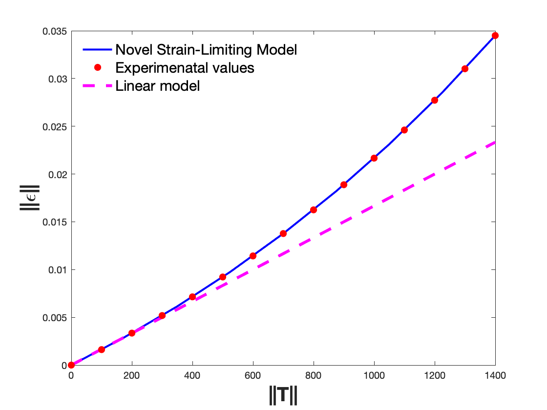
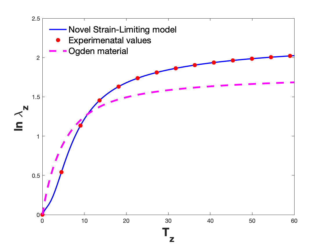
There are several experimental studies available in the literature [14, 45] which show the clear nonlinear stress-strain behavior for several materials such as gum metal [20], titanium alloys [51, 8], alloys such as Ti-30Nb-10Ta-5Zr (TNTZ-30). The nonlinear behavior is observed well within strain. Such behavior is traditionally modeled using a linear relationship between the “infinitesimal strain” and Cauchy stress using the classical linearized elasticity construct, which is odd as a linear relationship can’t fit the nonlinear data. The aforementioned nonlinear behavior can be modeled within the implicit theory of elasticity [39, 29, 17]. Rocks [5] and many rubber-like materials [6] can be modeled using a special subclass of models within the larger class of strain-limiting nonlinear relationships. In [6], a constitutive model for rubber is proposed using the principle stresses as the main variables, wherein a better corroboration with experimental data is shown than Ogden’s model [34]. The new material models studied by several aforementioned researchers are good candidates to fit the experimental data on gum metals, rubber-like materials, and high-strength titanium alloys [39, 8, 20, 6].
It is clear from the above Figure-1 that for some experiments, the classical linear model and the Ogden material model [34] can’t best fit the nonlinear behavior in the “small strain” regime (less than strains). Therefore, there is a great opportunity for modelers and computational scientists to develop new constitutive relationships that can correctly describe the experimentally observed phenomenon in many high-strength materials used in the construction industry, orthopedic implants, and aerospace applications.
3 Boundary value problem and existence of solution
We assume that the response of the body is constituted through the algebraically nonlinear relationship whereas the material is still geometrically linear. We suppose that the solid body is homogeneous and initially unstressed. Let where is a simply connected domain with its boundary being . The boundary consists of two non-overlapping parts and . Both of these boundary parts may contain finitely many parts and one can parameterize each one of them. Let be the space of all Lebesgue integrable functions with and denotes the inner product and be the corresponding induced norm. The classical Sobolev space is denoted by with the norm defined through:
and let denote the dual space to . We also define the following subspaces of
| (22) |
The out-of-plane displacement function is the only unknown variable that defines the mechanics of the material body. For the loading setup on hand, we have only two non-zero components in both stress and strain tensors. The problem under consideration is simplified to
Strong formulation.
Given the material parameter , find such that
| (23a) | ||||
| (23b) | ||||
In the above formulation, we have turned an original traction and displacement problem into a pure non-homogeneous Dirichlet-type problem for one single function . Our formulation is similar to the one studied in [2, 3, 20, 18, 55].
A well-posed weak formulation is derived from the above strong formulation by multiplying (23a) by test function and integrating by parts over the domain .
Continuous weak formulation.
Given the material parameter , find such that
| (24) |
The above continuous weak formulation has been shown to possess a unique solution. Here we recast the main theorem in [3] to gain a useful result about the existence and uniqueness of the solution to our formulation. We have the following theorem from [3]:
Theorem 1.
is a simply connected domain with boundary consisting of two subsets so that , where is the tangent to the boundary. Both the boundaries may consist of finitely many parts and each can be parameterized to an open interval. Each part in is flat. There exists a function such that . Let , then there is a unique solution for the problem satisfying
| (25a) | ||||
| (25b) | ||||
The above theorem is the same as the one proved in [3] has two additional modeling parameters and , however, for and our continuous formulation falls well within the purview of the proof achieved in [3]. Hence our continuous weak formulation in (24) is well-posed with the existence of a unique solution.
The above strong formulation doesn’t possess any exact analytical solution, even in the simpe setting of 1D. Therefore we look at developing a stable convergent numerical method using finite element discretization to approximate the solution to the weak formulation (24). In the next section, we propose a stable finite-element discretization in which the shape functions are calculated by using a one-of-its-kind point transformation. The exact transformation and the integration procedure produce superior numerical results.
4 Finite element discretization
In this contribution, we propose a finite element discretization of a nonlinear BVP that models the response of a strain-limiting elastic material containing both v-notch and inclusions. For the numerical approximation, the challenges are the mesh discretization and the PDE approximation. In the case of triangulation of the domain, we utilize the curved triangular elements which do not contain discretization error since the exact geometry is utilized in creating the finite element mesh. For the numerical approximation, cubic-order shape functions are adapted and these are obtained from one-of-its-kind point transformation established in the literature [27, 44]. The effective use of the higher order curved triangular elements are clearly demonstrated in works of [48, 50, 30, 49, 31, 32] An exact analytical solution is not known for the physical setup considered in this paper. Hence we compute a relative difference of the numerical solution between two successive Picard iterations as a measure to quantify the quality of the approximation proposed.
Let be a two-dimensional open domain with being its boundary which is assumed to be sufficiently smooth. The boundary is composed of the sets and such with being the number of inclusions. Here is the part where we apply the Dirichlet boundary condition and are the internal inclusions. The internal inclusions are assumed to be traction-free. The region near the holes is triangulated using “curved” triangles which contain one-side curved and two-side straight lines.
For approximating the displacement field , we define the following space,
| (26) |
where is a set of tensor-products of polynomials up to an order of over the reference cell . Then the discrete approximation space is
| (27) |
4.1 Construction of shape functions
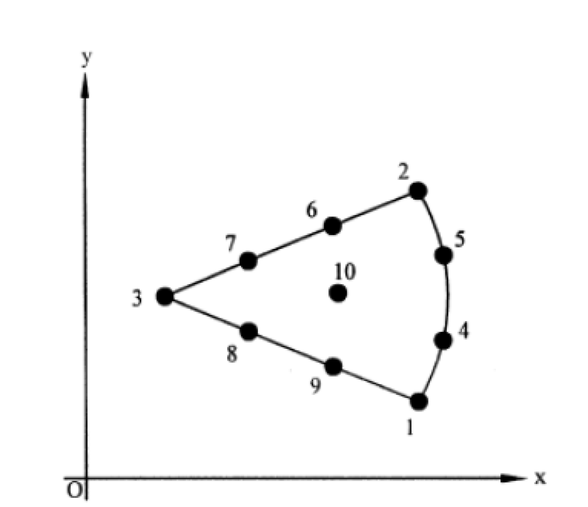
Consider the triangular elements in which one of the sides is curved and the other two sides are straight as shown in Fig. 2. The Lagrange interpolants for the field variable governing the physical problem are
| (28) |
where refers to the conventional triangular element shape functions Eq.(32) as derived in [27, 44] of order at the node . Hence the transformation formulae between the physical (Cartesian) and the local (natural) coordinate systems are
| (29) |
The nodes along the straight sides and in Fig.2 are equispaced. Now if we use the standard formulae dividing a line segment in a given ratio from the plane analytical geometry to the straight sides and then the Eq.(29) reduces to
| (30) |
where is the nodal value of the triangular element and is the well-known Heaviside step function or unit step function and it has the meaning for the present as,
| (31) |
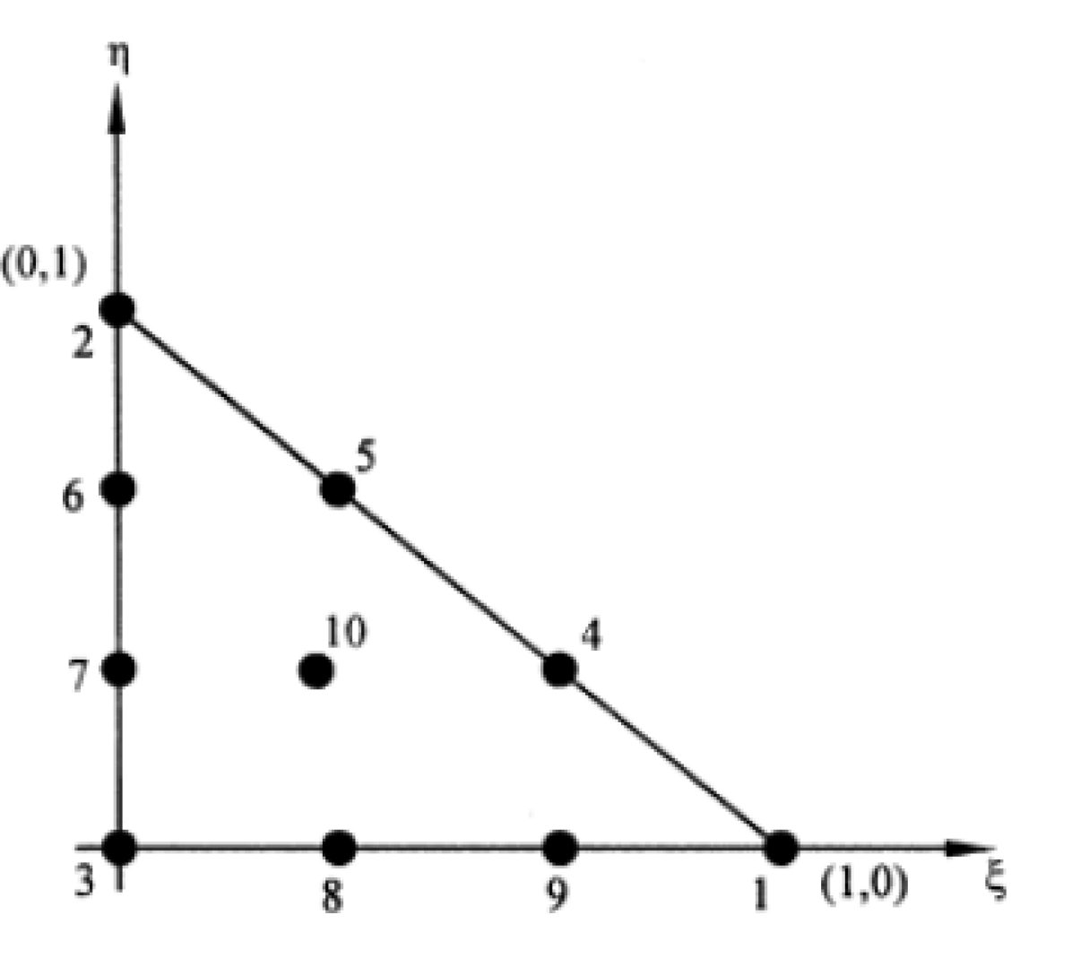
The following are the shape functions for a curved triangle element of cubic order:
| (32a) | ||||
| (32b) | ||||
| (32c) | ||||
| (32d) | ||||
| (32e) | ||||
| (32f) | ||||
| (32g) | ||||
| (32h) | ||||
| (32i) | ||||
| (32j) | ||||
Figure 2 depicts the domain with two straight sides and one curved side. The subparametric transformations given below are used to convert the global coordinates of a typical triangle element in cubic order to the local coordinates. The cubic order’s point transformation is as follows:
| (33) |
with the boundary node as,
| (34) |
and the interior node as,
| (35) |
4.2 Discrete formulation and Picard’s iteration
Starting with the continuous formulation, the discrete weak formulation is obtained using the shape functions from the approximation space defined in (27). However, the difficulty is in handling the nonlinearities in the continuous case. These can be handled either at the differential equation level or at the linear algebra level. We have used the former method by the well-known Picard’s type linearization. Such a linearization produces a sequence of linear problems. For fast convergence of the above iterative algorithm, a proper initial guess is required. In our implementation, we solved the linear problem first (obtained from (36) without the denominator) and subsequently used the computed solution as an initial guess for Picard’s iterations. All our numerical simulations converged within a reasonable number of iterations. Overall, our formulation possesses a unique solution at the discrete level. Finally, the discrete finite element problem reads:
Discrete Finite Element Problem.
Given the Dirichlet boundary data , and the iteration solution , for , find such that
| (36) |
where the bilinear and linear terms are given by
| (37a) | ||||
| (37b) | ||||
In the above weak formulation, the term is the known function and is the applied traction.
The following algorithm depicts the overall discrete finite element computational procedure to obtain the numerical solution of the BVP.
5 Numerical Examples
To illustrate the efficiency of the proposed method, we consider three examples: the first one consists of nonlinear BVP with a manufactured solution; the second one is the nonlinear BVP on the v-notch domain; the third one is the nonlinear BVP on the v-notch domain containing several inclusions. The challenge in the third example is the meshing near the curved inclusions. The proposed method takes very few elements to discretize the region near inclusions, more importantly, there is no discretization error due to considering curved triangles.
5.1 Square domain with a manufactured solution
In this example, we consider the nonlinear BVP posed on a square domain and we choose as the exact solution. The right-hand side term is computed by plugging into the strong form. The boundary values are set by using the manufactured solution . Such a situation allows us to do a convergence analysis in the standard measure. The computational domain is depicted in Figure 3. The boundary conditions are shown in the Table 1.
| Boundary | Values |
|---|---|
| 0 | |
For the illustrative purpose, we have considered three different types of meshes for computations. The mesh information is given in the following table:
| Elements | DOF | Boundary Nodes |
|---|---|---|
| 8 | 49 | 24 |
| 16 | 85 | 24 |
| 32 | 169 | 48 |
The discretization of the mesh using different numbers of elements is given in Figure 4.
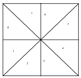
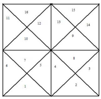
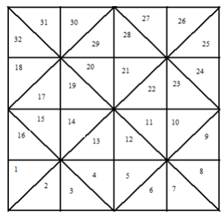
The plot of the numerical solution is given in Figure 5.
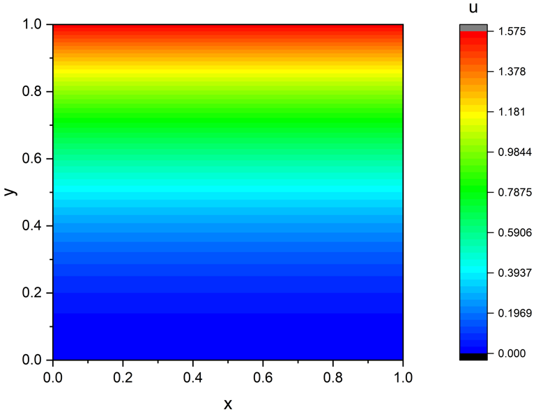
The following table indicates the convergence of the numerical solution for each of the computational meshes considered.
| Elements | -error norm | ||
|---|---|---|---|
| 8 | 0.000019 | ||
| 16 | 0.000023 | ||
| 32 | 0.000019 |
Here the symbols and are the absolute and relative errors, respectively. It is clear from Table 3 that our proposed finite element algorithm coupled with Picard’s type linearization is an excellent choice to approximate the solution to the class of quasilinear partial differential equation.
5.2 Domain with V-notch
In this example, our goal is to present an efficient numerical method for the discretization of the quasilinear boundary value problem on a domain containing V-notch. For this setup, we do not have an exact analytical solution. The geometry and the boundary indicators are shown in Figure 6. The boundary conditions are given in the Table 4.
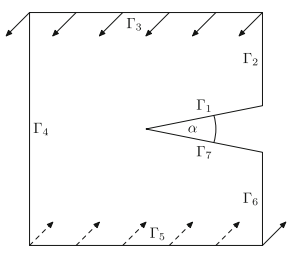
| Boundary | Values |
|---|---|
| 0 | |
| 0 | |
| 1 | |
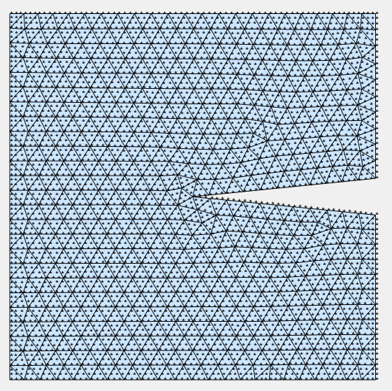
The computational mesh is depicted in Figure 7 and the corresponding information about the elements, degrees-of-freedom, and the number of boundary nodes is given in Table 6. The mesh size in our computational discretization is taken as .
| Elements | DOF | Boundary Nodes |
| 1038 | 4843 | 342 |
To monitor the convergence of our proposed method, we print out the maximum difference between the solutions at consecutive iterations. The computed values are given in the Table 6. For a consistent comparison, we have computed the relative difference at a particular node in the mesh.
| 0.079887041221999 |
| 0.041362782097059 |
| 0.021305707435756 |
| 0.011408306865723 |
| 0.006567123752435 |
| 0.003989228093075 |
| 0.002478142679311 |
| 0.001569657000410 |
| 0.001011378448757 |
| 0.000661660540590 |
| 0.000438859611370 |
| 0.000294760677603 |
| 0.000200279446002 |
| 0.000137545640890 |
| 0.000095400576785 |
| 0.000066775278713 |
| 0.000047132288683 |
| 0.000033523256409 |
| 0.000024010189043 |
| 0.000017305167042 |
| 0.000012543266832 |
| 0.000009137782930 |
The computed solution at the end of the Picard’s iteration is shown below in Figure 8.
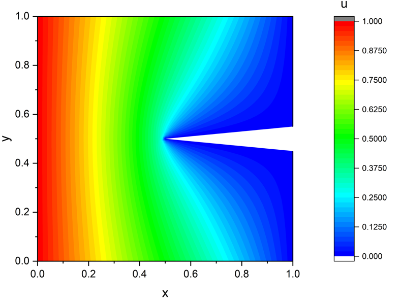
It is clear from Table 6 that our proposed method takes less than iterations to obtain a reasonably accurate numerical solution.
5.3 Domain with V-notch and inclusions
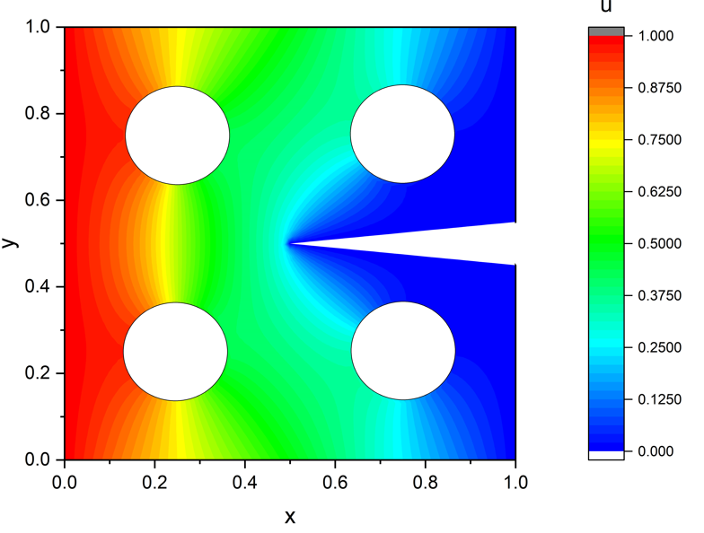
Here, our main objective is to present an efficient finite element method to handle the nonlinear partial differential equation posed on a domain containing v-notch and circular inclusions (or holes). The boundary conditions are kept the same as in the last example, and the inclusions are kept traction-free. The challenge for any numerical method is to handle the nonlinearities along with the triangulation of the domain. The proposed method studied in this paper considers the region near the inclusions as circular contrary to the other popular triangulations that use the points on the boundary of the inclusions to create the mesh with straight edges. The apparent bottleneck in many other finite element implementations is creating stable (good) computational mesh to efficiently evaluate the integrals needed to assemble the matrices and vectors. We do not have these issues as we do curved triangular elements along the circular inclusions. The triangulation of the domain is shown in Figure 9.
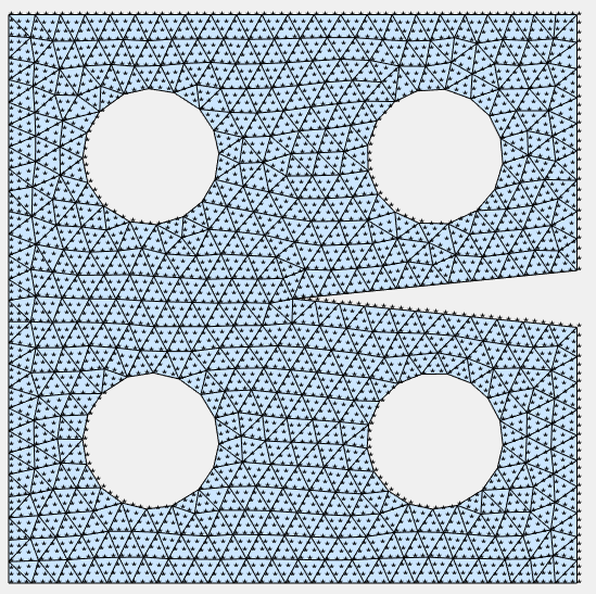
The statistics of the mesh are given in the following Table 8.
| Elements | DOF | Boundary Nodes |
| 836 | 4026 | 339 |
To monitor the convergence of the numerical solution, we compute the maximum difference between two consecutive solutions and the same is depicted in Table 8.
| 0.061362195377219 |
| 0.034003719699686 |
| 0.019375215579367 |
| 0.011322928480591 |
| 0.006773972907949 |
| 0.004099274297780 |
| 0.002509970577362 |
| 0.001554095858205 |
| 0.000983314280567 |
| 0.000642176317155 |
| 0.000423204575014 |
| 0.000281269726815 |
| 0.000188420856898 |
| 0.000127158649975 |
| 0.000086411758823 |
| 0.000059105537844 |
| 0.000040676772821 |
| 0.000028156283765 |
| 0.000019596217704 |
| 0.000013708893668 |
| 0.000009636885800 |
Figure 10 shows the plot of the finite element solution for a strain-limiting material body containing both v-notch and circular inclusions. The solution presented is the one obtained after Picard’s iteration and the overall algorithm met the stopping criteria.
6 Conclusion
An efficient finite element for simulating the response of the algebraically nonlinear and geometrically linear strain-limiting elastic material containing both v-notch and circular inclusions is presented. A boundary value problem consists of a second-order quasilinear partial differential equation obtained by considering a special constitutive relationship within the setting of a new theory formulated in [36, 42]. There are no analytical methods available to obtain a closed-form solution to such a setup. Hence, a novel type of finite element is proposed in this work. A general curved triangular element which is of cubic-order isoparametric type is utilized. Such curved elements are used along the circumference of the inclusions and which is adaptable to the analogous with the other triangular mesh elements in the bulk material body. A main element of our method is in approximating the curved boundary by second-order polynomials for the cubic order triangular method and also in constructing the efficient numerical method to approximate the primitive displacement variable. The proposed method is applied to three different boundary value problems. The accuracy of the numerical solution is tested against a manufactured solution. The numerical results obtained are very good and improve the accuracy of the approximation of the quasi-linear partial differential equation. The standard Picard’s type linearization takes less iteration to converge to the solution. Overall, the method presented in this paper is very good and crucial for several applications. The approach used to simulate the elastic material under mechanical loading can be easily adaptable to the quasi-static crack propagation both in elastic materials whose response is described by algebraically nonlinear relationship [54, 21] and in materials whose parameters dependent upon the density [56], multiscale situations [52, 53], and multi-physics problems [25].
References
- [1] A. Bonito, V. Girault, and E. Süli. Finite element approximation of a strain-limiting elastic model. IMA Journal of Numerical Analysis, 40(1):29–86, 2020.
- [2] M. Bulíček, J. Málek, K. R. Rajagopal, and E. Süli. On elastic solids with limiting small strain: modeling and analysis. EMS Surveys in Mathematical Sciences, 1(2), 2014.
- [3] M. Bulíček, J. Málek, K. R. Rajagopal, and J. R. Walton. Existence of solutions for the anti-plane stress for a new class of strain-limiting elastic bodies. Calculus of Variations and Partial Differential Equations, 54(2):2115–2147, 2015.
- [4] M. Bulíček, J. Málek, and E. Süli. Analysis and approximation of a strain-limiting nonlinear elastic model. Mathematics and Mechanics of Solids, 20(1):92–118, 2015.
- [5] R. Bustamante, S. Montero, and A. Ortiz-Bernardin. A novel nonlinear constitutive model for rock: Numerical assessment and benchmarking. Applications in Engineering Science, 3:100012, 2020.
- [6] R. Bustamante and K. R. Rajagopal. A new type of constitutive equation for nonlinear elastic bodies. fitting with experimental data for rubber-like materials. Proceedings of the Royal Society A, 477(2252):20210330, 2021.
- [7] P. G. Ciarlet and P.-A. Raviart. Interpolation theory over curved elements, with applications to finite element methods. Computer Methods in Applied Mechanics and Engineering, 1(2):217–249, 1972.
- [8] V. K. Devendiran, R. K. Sandeep, K. Kannan, and K. R. Rajagopal. A thermodynamically consistent constitutive equation for describing the response exhibited by several alloys and the study of a meaningful physical problem. International Journal of Solids and Structures, 108:1–10, 2017.
- [9] I. Ergatoudis, B. M. Irons, and O. C. Zienkiewicz. Curved, isoparametric,“quadrilateral” elements for finite element analysis. International Journal of Solids and Structures, 4(1):31–42, 1968.
- [10] L. A. Ferguson, M. Muddamallappa, and J. R. Walton. Numerical simulation of mode-iii fracture incorporating interfacial mechanics. International Journal of Fracture, 192:47–56, 2015.
- [11] K. Gou, M. Mallikarjuna, K. R. Rajagopal, and J. R. Walton. Modeling fracture in the context of a strain-limiting theory of elasticity: A single plane-strain crack. International Journal of Engineering Science, 88:73–82, 2015.
- [12] K. Gou and S. M. Mallikarjunaiah. Computational modeling of circular crack-tip fields under tensile loading in a strain-limiting elastic solid. Communications in Nonlinear Science and Numerical Simulation, 121:107217, 2023.
- [13] K. Gou and S. M. Mallikarjunaiah. Finite element study of v-shaped crack-tip fields in a three-dimensional nonlinear strain-limiting elastic body. Mathematics and Mechanics of Solids, page 10812865231152257, 2023.
- [14] Y. L. Hao, S. J. Li, S. Y. Sun, C. Y. Zheng, Q. M. Hu, and R. Yang. Super-elastic titanium alloy with unstable plastic deformation. Applied Physics Letters, 87(9):091906, 2005.
- [15] V. Kesavulu Naidu and K. V. Nagaraja. The use of parabolic arc in matching curved boundary by point transformations for septic order triangular element and its applications. Advanced Studies in Contemporary Mathematics, 20(3):437–456, 2010.
- [16] V. Kesavulu Naidu and K. V. Nagaraja. Advantages of cubic arcs for approximating curved boundaries by subparametric transformations for some higher order triangular elements. Applied Mathematics and Computation, 219(12):6893–6910, 2013.
- [17] K. Kowalczyk-Gajewska, E. A. Pieczyska, K. Golasiński, M. Maj, S. Kuramoto, and T. Furuta. A finite strain elastic-viscoplastic model of gum metal. International Journal of Plasticity, 119:85–101, 2019.
- [18] V. Kulvait, J. Malek, and K. R. Rajagopal. Anti-plane stress state of a plate with a v-notch for a new class of elastic solids. International Journal of Fracture, 179(1):59–73, 2013.
- [19] V. Kulvait, J. Málek, and K. R. Rajagopal. Modeling gum metal and other newly developed titanium alloys within a new class of constitutive relations for elastic bodies. Archives of Mechanics, 69(3), 2017.
- [20] V. Kulvait, J. Málek, and K. R. Rajagopal. The state of stress and strain adjacent to notches in a new class of nonlinear elastic bodies. Journal of Elasticity, 135(1):375–397, 2019.
- [21] S. Lee, H. C. Yoon, and S. M. Mallikarjunaiah. Finite element simulation of quasi-static tensile fracture in nonlinear strain-limiting solids with the phase-field approach. Journal of Computational and Applied Mathematics, 399:113715, 2022.
- [22] T. Mai and J. R. Walton. On monotonicity for strain-limiting theories of elasticity. Journal of Elasticity, 120(1):39–65, 2015.
- [23] T. Mai and J. R. Walton. On strong ellipticity for implicit and strain-limiting theories of elasticity. Mathematics and Mechanics of Solids, 20(2):121–139, 2015.
- [24] S. M. Mallikarjunaiah. On Two Theories for Brittle Fracture: Modeling and Direct Numerical Simulations. PhD thesis, Texas A&M University, 2015.
- [25] S. M. Mallikarjunaiah and D. Bhatta. A finite element model for hydro-thermal convective flow in a porous medium: Effects of hydraulic resistivity and thermal diffusivity. Under review, 2023.
- [26] S. M. Mallikarjunaiah and J. R. Walton. On the direct numerical simulation of plane-strain fracture in a class of strain-limiting anisotropic elastic bodies. International Journal of Fracture, 192(2):217–232, 2015.
- [27] R. J. Y. McLeod and A. R. Mitchell. The use of parabolic arcs in matching curved boundaries in the finite element method. IMA Journal of Applied Mathematics, 16(2):239–246, 1975.
- [28] A. R. Mitchell. Advantages of cubics for approximating element boundaries. Computers & Mathematics with Applications, 5(4):321–327, 1979.
- [29] A. Muliana, K. R. Rajagopal, D. Tscharnuter, B. Schrittesser, and G. Saccomandi. Determining material properties of natural rubber using fewer material moduli in virtue of a novel constitutive approach for elastic bodies. Rubber Chemistry and Technology, 91(2):375–389, 2018.
- [30] K. Murali, V. Kesavulu Naidu, and B. Venkatesh. Darcy–brinkman–forchheimer flow over irregular domain using finite elements method. IOP Conference Series: Materials Science and Engineering, 577(1):012158, nov 2019.
- [31] K Murali, V Kesavulu Naidu, and B Venkatesh. Solution of darcy-brinkman flow over an irregular domain by finite element method. Journal of Physics: Conference Series, 1172(1):012091, mar 2019.
- [32] K Murali, V Kesavulu Naidu, and B Venkatesh. Solution of darcy–brinkman–forchheimer equation for irregular flow channel by finite elements approach. Journal of Physics: Conference Series, 1172(1):012033, mar 2019.
- [33] K. V. Nagaraja, V. Kesavulu Naidu, and H. T. Rathod. The use of parabolic arc in matching curved boundary by point transformations for sextic order triangular element. International Journal of Mathematical Analysis, 4:357–374, 2010.
- [34] R. W. Ogden. Large deformation isotropic elasticity–on the correlation of theory and experiment for incompressible rubberlike solids. Proceedings of the Royal Society of London. A. Mathematical and Physical Sciences, 326(1567):565–584, 1972.
- [35] K. R. Rajagopal. On implicit constitutive theories. Applications of Mathematics, 48(4):279–319, 2003.
- [36] K. R. Rajagopal. The elasticity of elasticity. Zeitschrift für Angewandte Mathematik und Physik (ZAMP), 58(2):309–317, 2007.
- [37] K. R. Rajagopal. Conspectus of concepts of elasticity. Mathematics and Mechanics of Solids, 16(5):536–562, 2011.
- [38] K. R. Rajagopal. Non-linear elastic bodies exhibiting limiting small strain. Mathematics and Mechanics of Solids, 16(1):122–139, 2011.
- [39] K. R. Rajagopal. On the nonlinear elastic response of bodies in the small strain range. Acta Mechanica, 225(6):1545–1553, 2014.
- [40] K. R. Rajagopal and A. R. Srinivasa. On thermomechanical restrictions of continua. Proceedings of the Royal Society of London. Series A: Mathematical, Physical and Engineering Sciences, 460(2042):631–651, 2004.
- [41] K. R. Rajagopal and A. R. Srinivasa. On a class of non-dissipative materials that are not hyperelastic. In Proceedings of the Royal Society of London A: Mathematical, Physical and Engineering Sciences, volume 465, pages 493–500. The Royal Society, 2009.
- [42] K. R. Rajagopal and J. R. Walton. Modeling fracture in the context of a strain-limiting theory of elasticity: a single anti-plane shear crack. International journal of fracture, 169(1):39–48, 2011.
- [43] KR Rajagopal and A. R. Srinivasa. On the response of non-dissipative solids. Proceedings of the Royal Society A: Mathematical, Physical and Engineering Sciences, 463(2078):357–367, 2007.
- [44] H. T. Rathod, K. V. Nagaraja, V. Kesavulu Naidu, and B. Venkatesudu. The use of parabolic arcs in matching curved boundaries by point transformations for some higher order triangular elements. Finite Elements in Analysis and Design, 44(15):920–932, 2008.
- [45] T. Saito, T. Furuta, J.-H. Hwang, S. Kuramoto, K. Nishino, N. Suzuki, R. Chen, A. Yamada, K. Ito, Y. Seno, T. Nonaka, H. Ikehata, N. Nagasako, C. Iwamoto, Y. Ikuhara, and T. Sakuma. Multifunctional alloys obtained via a dislocation-free plastic deformation mechanism. Science, 300(5618):464–467, 2003.
- [46] J Sasikala, V. Kesavulu Naidu, B. Venkatesh, and S. M. Mallikarjunaiah. On an efficient octic order sub-parametric finite element method on curved domains. Computers & Mathematics with Applications, 143:249–268, 2023.
- [47] L. R. Scott. Finite element techniques for curved boundaries. PhD thesis, Massachusetts Institute of Technology, 1973.
- [48] G Shylaja, B Venkatesh, V Kesavulu Naidu, and K Murali. Improved finite element triangular meshing for symmetric geometries using matlab. Materials Today: Proceedings, 46:4375–4380, 2021.
- [49] G Shylaja, B Venkatesh, and V Kesavulu Naidu. Finite element method to solve poisson’s equation using curved quadratic triangular elements. IOP Conference Series: Materials Science and Engineering, 577(1):012165, nov 2019.
- [50] G. Shylaja, B. Venkatesh, V. Kesavulu Naidu, and K. Murali. Two-dimensional non-uniform mesh generation for finite element models using matlab. Materials Today: Proceedings, 46:3037–3043, 2021. International Conference on Advances in Material Science and Chemistry – 2020 (ICAMSC-2020).
- [51] Y. Tian, Z. Yu, C. Y. A. Ong, and W. Cui. Nonlinear elastic behavior induced by nano-scale phase in matrix of -type ti–25nb–3zr–2sn–3mo titanium alloy. Materials Letters, 145:283–286, 2015.
- [52] M. Vasilyeva and S. M. Mallikarjunaiah. Generalized multiscale finite element treatment of a heterogeneous nonlinear strain-limiting elastic model. Multiscale Modeling & Simulation, 22(1):334–368, 2024.
- [53] M. Vasilyeva, S. M. Mallikarjunaiah, and D. Palaniappan. Multiscale model reduction technique for fluid flows with heterogeneous porous inclusions. Journal of Computational and Applied Mathematics, 424:114976, 2023.
- [54] H. C. Yoon, S. Lee, and S. M. Mallikarjunaiah. Quasi-static anti-plane shear crack propagation in nonlinear strain-limiting elastic solids using phase-field approach. International Journal of Fracture, 227(2):153–172, 2021.
- [55] H. C. Yoon and S. M. Mallikarjunaiah. A finite-element discretization of some boundary value problems for nonlinear strain-limiting elastic bodies. Mathematics and Mechanics of Solids, 27(2):281–307, 2022.
- [56] H. C. Yoon, S. M. Mallikarjunaiah, and D. Bhatta. Finite element solution of crack-tip fields for an elastic porous solid with density-dependent material moduli and preferential stiffness. Accepted for publication in Advances in Mechanical Engineering, 2024.
- [57] H. C. Yoon, K. K. Vasudeva, and S. M. Mallikarjunaiah. Finite element model for a coupled thermo-mechanical system in nonlinear strain-limiting thermoelastic body. Communications in Nonlinear Science and Numerical Simulation, 108:106262, 2022.
- [58] O. C. Zienkiewicz and R. L. Taylor. The finite element method for solid and structural mechanics. Elsevier, 2005.
