Fairness Risks for Group-Conditionally Missing Demographics

Abstract

Fairness-aware classification models have gained increasing attention in recent years as concerns grow on discrimination against some demographic groups. Most existing models require full knowledge of the sensitive features, which can be impractical due to privacy, legal issues, and an individual’s fear of discrimination. The key challenge we will address is the group dependency of the unavailability, e.g., people of some age range may be more reluctant to reveal their age. Our solution augments general fairness risks with probabilistic imputations of the sensitive features, while jointly learning the group-conditionally missing probabilities in a variational auto-encoder. Our model is demonstrated effective on both image and tabular datasets, achieving an improved balance between accuracy and fairness.

1 Introduction

As machine learning systems rapidly acquire new capabilities and get widely deployed to make human-impacting decisions, ethical concerns such as fairness have recently attracted significant effort in the community. To combat societal bias and discrimination in the model that largely inherit from the training data, a bulk of research efforts have been devoted to addressing group unfairness, where the model performs more favorably (e.g., accurately) to one demographic group than another (Buolamwini & Gebru, 2018; Gianfrancesco et al., 2018; Mehrabi et al., 2021; Yapo & Weiss, 2018). Group fairness typically concerns both the conventional classification labels (e.g., recidivism) and socially sensitive group features (e.g., age, gender, or race). As applications generally differ in their context of fairness, a number of quantitative metrics have been developed such as demographic parity, equal opportunity, and equalized odds. A necessarily outdated overview is available at Barocas et al. (2019) and Wikipedia contributors (2024).

Learning algorithms for group fairness can be broadly categorized into pre-, post-, and in-processing methods. Pre-processing methods transform the input data to remove dependence between the class and demographics according to a predefined fairness constraint (Kamiran & Calders, 2012). Post-processing methods warp the class labels (or their distributions) from any classifier to fulfill the desired fairness criteria (Hardt et al., 2016). In-processing approaches, which are most commonly employed including this work, learn to minimize the prediction loss while upholding fairness regularizations simultaneously. More discussions are relegated to Section 2.

Most of these methods require accessing the sensitive demographic feature, which is often unavailable due to fear of discrimination and social desirability (Krumpal, 2013), privacy concerns, and legal regulations (Coston et al., 2019; Lahoti et al., 2020). For example, mid-aged people may be more inclined to withhold their age information when applying for entry-level jobs, compared with younger applicants. Recently several methods have been developed for this data regime. Lahoti et al. (2020) achieved Rawlsian max-min fairness by leveraging computationally-identifiable errors in adversarial reweighted learning. Hashimoto et al. (2018) proposed a distributionally robust optimization to minimize the risk over the worst-case group distribution. However, they are not effective in group fairness and cannot be customized for different group fairness metrics. Yan et al. (2020) infers groups by clustering the data, but there is no guarantee that the uncovered groups are consistent with the real sensitive features of interest. For example, the former may identify race while we seek to be fair in gender.

We seek to address these issues in a complementary setting, where demographics are partially missing. Although their availability is limited, it is still often feasible to obtain a small amount of labeled demographics. For example, some people may not mind disclosing their race or gender. Therefore, different from the aforementioned works that assume complete unavailability of demographics, we study in this paper the semi-supervised setting where they can be partially available at random in both training and test data. Similarly, the class labels can be missing in training.

Semi-supervised learning has been well studied, and can be applied to impute missing demographics. Zhang & Long (2021) simply used the fully labeled subset to estimate the fairness metrics, but their focus is on analyzing its estimation bias instead of using it to train a classifier. Jung et al. (2022) assigned pseudo group labels by training an auxiliary group classifier, and assigned low-confidence samples to random groups. However, the confidence threshold needs to be tuned based on the conditional probability of groups given the class label, which becomes challenging as the latter is also only partially available in our setting.

Dai & Wang (2021) used semi-supervised learning on graph neural networks to infer the missing demographics, but rounded the predictions to binary group memberships. This is suboptimal because, due to the scarcity of labeled data, there is marked uncertainty in demographic imputations. As a result, the common practice of “rounding” sensitive estimates—so that fairness metrics defined on categorical memberships can be enforced instead of mere independence—may over-commit to a group just by chance, dropping important uncertainty information when the results are fed to downstream learners. Moreover, most applications do not naturally employ an underlying graph, and the method only enforces min-max (i.e., adversarial) fairness instead of group fairness metrics.

Our first contribution, therefore, is to leverage the probabilistic imputation by designing a differentiable fairness risk in Section 4, such that it is customized for a user-specified fairness metric with discrete demographics as opposed to simple independence relationships, and can be directly integrated into general semi-supervised learning algorithms to regularize the learned posterior towards low risks in both classification and fairness. We also addressed pathological solutions arising from jointly learning group memberships.

As our second contribution, we instantiated the semi-supervised classifier with a new encoder and decoder in a variational autoencoder (VAE, Narayanaswamy et al., 2017; Kingma et al., 2014), allowing group-conditional missing demographics, which has so far only been considered for noisy but not missing demographics. In general, the chance of unavailability does depend on specific groups – if people of a certain race are aware of the unfairness against them, they will be more reluctant to disclose their race. The comprehensive model will be introduced in Section 5.

Risk-based models generally require nontrivial techniques for efficient inference and differentiation, because most fairness metrics do not factor over examples’ predictions. Hence, our third contribution is to address this issue in Section 4.3 through a Monte-Carlo approach, proffering $O(1/\epsilon^{2})$ sample complexity.

Our fourth contribution is to demonstrate, in Section 6, that our method empirically outperforms state of the art for fair classification where both the demographics and class labels are only partially available. The paper’s technical development will be primed with preliminaries in Section 3.

2 Related Work

Noisy demographics have been addressed by, e.g., Lamy et al. (2019) and Celis et al. (2021a). Celis et al. (2021b) and Mozannar et al. (2020) studied adversarially perturbed and privatized demographics. They also account for group-conditional noise. However, although they conceptually subsume unavailability as a special type of noise, their method and analysis do not carry through. Some of these methods, along with Wang et al. (2020), also require an auxiliary dataset to infer the noise model, which is much harder for missing demographics. Shah et al. (2023) dispenses with such a dataset, but its favorable theoretical properties only apply to Gaussian data, while the bootstrapping-based extension to non-Gaussian data does not model the conditional distribution of demographics.

Another strategy to tackle missing demographics resorts to proxy features (Gupta et al., 2018; Chen et al., 2019; Kallus et al., 2022). Based on domain knowledge, they are assumed to correlate with and allude to the sensitive feature in question. Zhao et al. (2022) optimizes the correlations between these features and the prediction, but it is not tailored to the specific group fairness metric in question. This is difficult because it relies on the binary group memberships which is not modeled by the method. Zhu et al. (2023) considered the accuracy of estimating the fairness metrics using proxies, but did not demonstrate its effectiveness when applied to train a fair classifier. In addition, proxy features can often be difficult to identify. In face recognition where the sensitive feature is age, race, or wearing glasses, raw pixels are no good proxies and identifying semantic features as proxies can be challenging.

3 Preliminary

We first consider supervised learning with group fairness, where samples are drawn from a distribution $D$ over $\mathcal{X}\times\{0,1\}\times\{0,1\}$, with $(X,A,Y)\sim D$. Here $X$ is the non-protected feature, $Y$ is the binary label, and $A$ is the binary sensitive feature which is also referred to as the group demographics. Our method can be extended to multi-class labels and sensitive features, provided that the fairness risk can be defined under fully observed $A$ and $Y$. Since our focus is on addressing the missing demographics, we will stick with the binary formulation just for ease of exposition.

We follow the setup in Menon & Williamson (2018) and aim to find a measurable randomized classifier parameterized by a function $f:\mathcal{X}\to[0,1]$ (e.g., neural network), such that it predicts an $x\in\mathcal{X}$ to be positive with probability $f(x)$. That is, the predicted label $\hat{Y}\in\{0,1\}$ follows the Bernoulli distribution $\hat{Y}|X\sim\text{Bern}(f(X))$. We denote the conditional distribution as $P_{f}(\hat{Y}|X)$, and omit the subscript $f$ for brevity when the context is clear. This setup also subsumes a classifier based on a class-probability estimator, where $f(X)\in[0,1]$ is translated to a hard deterministic label via a learnable threshold $\tau$: $P_{f}(\hat{Y}=1|X)=[\![f(X)>\tau]\!]$. Here, the Iverson bracket $[\![\cdot]\!]=1$ if $\cdot$ is true, and 0 else.

Suppose we have a training set $\mathcal{D}_{tr}:=\{\mathbf{\bm{x}}_{i},y_{i},a_{i}\}_{i=1}^{n}$. In the completely observed scenario, both $y_{i}$ and $a_{i}$ are in $\{0,1\}$. However, in the sequel, we will also consider the cases where the label and/or demographic is missing for some examples. In such cases, we denote $y_{i}$ or $a_{i}$ as $\emptyset$. As a shorthand, let $\mathbf{\bm{a}}=(a_{1},\ldots,a_{n})^{\top}$ and $\mathbf{\bm{y}}=(y_{1},\ldots,y_{n})^{\top}$.

We first review some standard group fairness concepts. The demographic parity is defined as

$$P(\hat{Y}=1|A=0)=P(\hat{Y}=1|A=1).$$ (1)

Similarly, we can define equalized odds as

$$P(\hat{Y}=1|A=0,Y=y)=P(\hat{Y}=1|A=1,Y=y)\!\!\!$$ (2)

for all $y\in\{0,1\}$, and equal opportunity as

$$P(\hat{Y}=1|A=0,Y=1)\!=\!P(\hat{Y}=1|A=1,Y=1).\!\!\!$$ (3)

In general, enforcing perfect fairness can be too restrictive, and approximate fairness can be considered via fairness measures. For example, the mean difference compares their difference (Calders & Verwer, 2010)

$$\text{MD}(f)=P(\hat{Y}=1|A=0)-P(\hat{Y}=1|A=1).$$ (4)

and the disparate impact (DI) factor computes their ratio (Feldman et al., 2015). Similar measures can be defined for equal opportunity and equalized odds. For continuous variables, $\chi^{2}$-divergence measures the independence as stipulated by separation and independence (Mary et al., 2019).

Given a dataset $\mathcal{D}_{tr}$ with finite samples, we can empirically estimate both sides of (1) by, e.g.,

$$P(\hat{Y}=1|A=a)\ \approx\ \text{mean}_{i}\{P_{f}(\hat{Y}=1|x_{i}):a_{i}=a\},$$

where $a\in\{0,1\}$. This mean estimator is straightforward from Eq 1 and 7 of Menon & Williamson (2018) in the setting of randomized classifier, and it is unbiased, consistent, and differentiable with respect to $f$. Similarly, $P(\hat{Y}=1|A=a,Y=y)$ can be estimated by

$$\text{mean}_{i}\{P_{f}(\hat{Y}=1|x_{i}):a_{i}=a,y_{i}=y\}.$$

Other estimation methods can also be adopted, such as kernel density estimation (Cho et al., 2020). Applying these estimates to MD, DI, $\chi^{2}$-divergence, or any other metric, we obtain a fairness risk $\mathcal{F}(P_{f},\mathbf{\bm{y}},\mathbf{\bm{a}})$.

Classification risk.

We denote the conventional classification risk as $\mathcal{R}(P_{f},\mathbf{\bm{y}})$. For example, the standard cross-entropy loss yields $-\frac{1}{n}\sum_{i}\log P_{f}(\hat{Y}=y_{i}|X=x_{i})$. Combined with fairness risk, we can proceed to find the optimal $f$ by minimizing their sum:

$$\mathcal{F}(P_{f},\mathbf{\bm{y}},\mathbf{\bm{a}})+\lambda\cdot\mathcal{R}(P_{f},\mathbf{\bm{y}}),$$ (5)

where $\lambda\!>\!0$ a trade-off hyperparameter. In Williamson & Menon (2019), a more general framework of fairness risk is constructed, incorporating the loss $\ell$ into the definition of $\mathcal{F}$ itself (Lahoti et al., 2020). Our method developed below can be applied there directly.

4 Fairness Risks with Group-Conditionally Unavailable Demographics

The regularized objective (5) requires the demographic features which can often become unavailable due to a respondent’s preference, privacy, and legal reasons. As a key contribution of this work, we further address group-conditionally unavailable demographics, where the demographics can get unavailable in a non-uniform fashion, i.e., depending on the specific group. This is quite realistic in practice. For example, individuals of some gender may be more reluctant to reveal their age for some applications.

We show that this new setting can be addressed by extending the objective (5). To this end, we introduce a new random variable $\tilde{A}$, which is the observation of the true latent demographic $A$. For a principled treatment, we treat $A$ as never observed, while $\tilde{A}$ can be equal to $A$, or take a distorted value, or be unavailable (denoted as $\emptyset$). In other words, $\tilde{A}$ is always observed, including taking the value of $\emptyset$.

We model the group-conditional unavailability with a learnable noising probability $P(\tilde{A}|A)$ (Yao et al., 2023). As a special case, one may assert that demographics cannot be misrepresented, i.e., $P(\tilde{A}|A)=0$ for all $\tilde{A}\notin\{A,\emptyset\}$. In order to address isometry (e.g., totally swapping the concept of male and female), we need to impose some prior on $P(\tilde{A}|A)$. For example, its value must be low for $\tilde{A}\notin\{A,\emptyset\}$. This can be enforced by a Dirichlet prior, e.g., $(P(\text{male}|\text{male}),P(\text{female}|\text{male}),P(\emptyset|\text{male}))\sim\text{Dir}(0.5,0.1,0.4)$. Similarly, we can define $P(\tilde{Y}|Y)$ for class-conditionally unavailable label, allowing $\tilde{Y}=\emptyset$.

In the sequel, we will assume there is already a semi-supervised learning algorithm that predicts $Y$ and $A$ with probabilistic models $P_{f}(Y|X,\tilde{Y})$ and $q_{\phi}(A|X,\tilde{A})$, respectively. For example, the encoder of a variational auto-encoder (VAE), which will be detailed in Section 5. It is now natural to extend the fairness risk by taking the expectation of these missing values:

$$\mathcal{E}_{\text{vanilla}}(P_{f},q_{\phi}):=$$ (6)

$$\qquad\mathop{\mathbb{E}}\limits_{Y_{i}\sim P_{f}(Y|x_{i},{\tilde{y}}_{i})}\mathop{\mathbb{E}}\limits_{A_{i}\sim q_{\phi}(A|x_{i},{\tilde{a}}_{i})}\mathcal{F}(P_{f},Y_{1:n},A_{1:n}).$$

In the case of no misrepresentation, the expectation of $A_{i}$ can be replaced by $A_{i}={\tilde{a}}_{i}$ if ${\tilde{a}}_{i}\neq\emptyset$. Likewise for $Y_{i}$. Adding this vanilla semi-supervised regularizer to an existing learning objective of $P_{f}$ and $q_{\phi}(A|X,\tilde{A})$ such as VAE gives a straightforward promotion of fairness, and we will also discuss its optimization in Section 4.4. However, despite its clear motivation, we now demonstrate that it is indeed plagued with conceptual and practical issues, which we will address next.

4.1 Rationalizing the semi-supervised fairness risk

It is important to note that the onus of fairness is only supposed to be on the classifier $P_{f}$, while $q_{\phi}(A|X,\tilde{A})$—which infers the demographics to define the fairness metric itself—is supposed to be recused from fairness risk minimization. Reducing the risk by manipulating an individual’s gender is not reasonable. This issue does not exist in a fully supervised setting, but complicates the regularizer when $q_{\phi}(A|X,\tilde{A})$ is jointly optimized with the classifier $P_{f}$. For example, although the risk can be reduced by making $A$ independent of $X$, this should not be intentionally pursued unless the underlying data distribution supports it. The posterior $q_{\phi}(A|X,\tilde{A})$ is only supposed to accurately estimate the demographics, while the task of fairness should be left to the classifier $P_{f}$.

A natural workaround is a two-step approach: first train a semi-supervised learner for the distribution $A|X,\tilde{A}$, and denote it as $r(A|X,\tilde{A})$. Then in (6), we replace $A_{i}\sim q_{\phi}(A|x_{i},{\tilde{a}}_{i})$ with $A_{i}\sim r(A|x_{i},{\tilde{a}}_{i})$. Although this resolves the above issue, it decouples the learning of $A|X,\tilde{A}$ (first step) and $Y|X,\tilde{Y}$ (second step). This is not ideal because, as commonly recognized, the inference of $A$ and $Y$ can benefit from shared backbone feature extractors on $X$ (e.g., ResNet for images), followed by finetuning the heads that cater for different targets.

However, sharing backbones will allow $q_{\phi}(A|X,\tilde{A})$ to be influenced by the learning of $P_{f}(Y|X,\tilde{Y})$, conflicting with the aforementioned recusal principle. In light of this difficulty, we resort to the commonly used stop-gradient technique that is readily available in PyTorch and TensorFlow. While they still share backbones, the derivative of $\mathcal{E}_{\text{vanilla}}$ in (6) with respect to $q_{\phi}(A|X,\tilde{A})$ is stopped from backpropagation, i.e., treating $q_{\phi}(A|X,\tilde{A})$ as a constant. It also simplifies the training process by avoiding two steps.

4.2 Imputation of unavailable training labels

A similar issue is also present in the expectation $Y_{i}\sim P_{f}(Y|x_{i},{\tilde{y}}_{i})$ in (6). The ground truth label $Y_{1:n}$ is given in the supervised setting, but its missing values should not be inferred to account for fairness, because labels are part of the fairness definition itself, except for demographic parity. We could resort to the stop-gradient technique again to withhold the backpropagation through $Y_{i}\sim P_{f}(Y|x_{i},{\tilde{y}}_{i})$. However, different from unavailable demographics, the situation here is more intricate because $P_{f}$ also serves as the first argument of $\mathcal{F}(P_{f},Y_{1:n},A_{1:n})$, where it indeed enforces fair classification. This conflicts with the fairness-oblivious requirement for imputing $Y_{i}$, which is also based on $P_{f}$. In other words, we cannot enforce $P_{f}$ to both respect and disregard fairness at the same time.

To address this issue, we will train a separate semi-supervised classifier to impute $Y_{i}$ without fairness concerns, and it does leverage the backbone features mentioned above. Suppose $\mathbf{\bm{h}}_{i}$ is the current feature representation for $x_{i}$, e.g., the third last layer of $f$. Assuming there is no misrepresentation in ${\tilde{y}}_{i}$, we can clamp $Y|x_{i}$ to $P_{f}$ for those examples with observed label (${\tilde{y}}_{i}\neq\emptyset$). Then we infer a class probability ${\color[rgb]{1,0,0}P_{g}}(Y|x_{i})$ for the rest examples by using $\mathbf{\bm{h}}_{i}$ and any semi-supervised learning algorithm such as graph-based Gaussian field (Zhu et al., 2003). This amounts to a fairness risk as

$$\boxed{\mathcal{E}(P_{f},q_{\phi})}:=$$ (7)

$$\qquad\mathop{\mathbb{E}}\limits_{\{Y_{i}\sim{\color[rgb]{1,0,0}P_{g}}(Y|x_{i}):{\tilde{y}}_{i}=\emptyset\}}\mathop{\mathbb{E}}\limits_{A_{i}\sim{\color[rgb]{1,0,0}q_{\phi}}(A|x_{i},{\tilde{a}}_{i})}\mathcal{F}(P_{f},Y_{1:n},A_{1:n}).$$

Note we stop the gradient on $P_{g}$ and $q_{\phi}$ here, and $P_{g}$ is used instead of $P_{f}$.

This risk can also be extended from randomized classifier to class-probability estimator; see Appendix A.5.

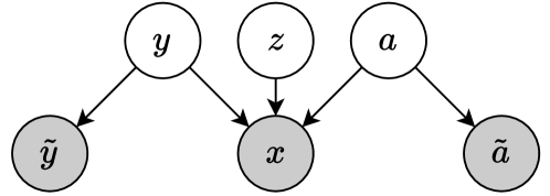
(a) Decoder

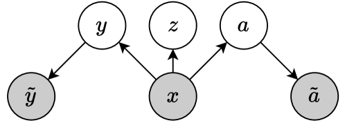
(b) Encoder

Figure 1: Decoder and encoder of SS-VAE with unavailable demographics/label conditioned on group/class.

4.3 Efficient evaluation of fairness risk $\mathcal{E}$

A major challenge in risk-based methods is the cost of computing the expectations in $\mathcal{E}$, along with its derivatives. In the sequel, we will resort to a Monte Carlo based method, such that for $n$ training examples, an $\epsilon$ accurate approximation with confidence $1-\delta$ can be found with $O(\frac{c_{n}}{\epsilon^{2}}\log\frac{1}{\delta})$ computation, where $c_{n}$ is the cost of evaluating $\mathcal{F}$ and it is $O(n)$ in our considered cases. Although some customized algorithms can be developed by exploiting the specific structures in $\mathcal{F}$ such as demographic parity, we prefer a more general approach based on sampling. Despite the inevitable inexactness in the result, we prove tight concentration bounds that turn out sufficiently accurate in practice.

Our method simply draws $N$ number of iid samples from $A_{i}\sim q_{\phi}(A|x_{i},{\tilde{a}}_{i})$ and $Y_{i}\sim P_{g}(Y|x_{i})$. For $s=1,\ldots,N$, let $Z_{s}:=\{a^{(s)}_{i},y^{(s)}_{i}\}_{i=1}^{n}$. We estimate $\mathcal{E}$ by

$$\hat{\mathcal{E}}_{n}(Z_{1},\ldots,Z_{N}):={\textstyle\frac{1}{N}}\sum\nolimits_{s=1}^{N}\mathcal{F}(P_{f},Z_{s}).$$ (8)

We prove the following sample complexity for this estimator by leveraging McDiarmid’s inequality.

Theorem 1.

Suppose $\mathcal{F}\in[0,C]$. Then for all $\epsilon>0$,

$$P(|\hat{\mathcal{E}}_{n}(Z_{1},\ldots,Z_{N})-\mathcal{E}|\geq\epsilon)\leq\ 2\exp(-2N\epsilon^{2}/C^{2}).$$

As a result, to guarantee an estimation error of $\epsilon$ with confidence $1-\delta$, it suffices to draw $N=\frac{C^{2}}{2\epsilon^{2}}\log\frac{1}{\delta}$ samples. The proof is available in Appendix A.1.

As $\hat{\mathcal{E}}_{n}(Z_{1},\ldots,Z_{N})$ costs $O(nN)$ to compute, the total cost is $\frac{nC^{2}}{2\epsilon^{2}}\log\frac{2}{\delta}$. When $C=1$, $\epsilon=0.01$ and $n=10^{4}$, this is just order of $10^{8}$, which is very much affordable. In experiments, a sample size $N$ as low as 100 was sufficient for our method to outperform the state of the art; see Section 6.2. Most risks we consider satisfy the boundedness assumption, although exceptions also exist such as disparate impact.

4.4 Differentiation of vanilla fairness risk

Since we stop the gradient with respect to $q_{\phi}(A|x_{i},{\tilde{a}}_{i})$ and $P_{g}(Y|x_{i})$, the whole regularizer $\mathcal{E}(P_{f},q_{\phi})$ in (7) can be easily differentiated with respect to $f$.

In practice, we also would like to conduct an ablation study by comparing with $\mathcal{E}_{\text{vanilla}}$, where challenges arise from differentiation with respect to $q_{\phi}(A|x_{i},{\tilde{a}}_{i})$ and $y_{i}\sim P_{f}(Y|x_{i},{\tilde{y}}_{i})$. We resolve this issue by using the straight-through Gumbel-Softmax method (Jang et al., 2017; Maddison et al., 2017). A self-contained description is given in Appendix A.2.

5 Integrating Fairness Risk with Semi-supervised Learning

We next illustrate how the fairness risk can be integrated with semi-supervised learners. As an example, we recap the semi-supervised VAE (SS-VAE, Kingma et al., 2014) in the context of missing $a$ and/or $y$ values.

5.1 Encoders and decoders

SS-VAE employs a decoder/generation process and an encoder/inference process parameterized by $\theta$ and $\phi$ respectively. In the decoder whose graphical model is shown in Figure 1(a), the observation $\mathbf{\bm{x}}$ is generated conditioned on the latent variable $\mathbf{\bm{z}}$, latent class $y$ and latent demographics $a$:

a

$$p_{\theta}(\mathbf{\bm{x}},{\tilde{a}},{\tilde{y}}|a,y,\mathbf{\bm{z}})=\mathcal{N}(\mathbf{\bm{x}}|g_{\theta}(a,y,\mathbf{\bm{z}}))\cdot P_{\theta}({\tilde{a}}|a)\cdot P_{\theta}({\tilde{y}}|y),$$

$$p(\mathbf{\bm{z}})=\mathcal{N}(\mathbf{\bm{z}}|0,I),$$

$$p(y)=\text{Cat}(y|\pi_{y}),\quad p(\pi_{y})=\text{SymDir}(\gamma_{y}),\quad$$ (9)

$$p(a)=\text{Cat}(a|\pi_{a}),\quad p(\pi_{a})=\text{SymDir}(\gamma_{a}).$$

Here $\text{Cat}(y|\pi_{y})$ is the multinoulli prior of the class variable. SymDir is the symmetric Dirichlet distribution with hyperparameter $\gamma_{y}$. The prior of $a$ is analogously defined.

The inference process finds conditionally independent representations $\mathbf{\bm{z}}$, $a$, and $y$ under a given $\mathbf{\bm{x}}$, ${\tilde{a}}$, and ${\tilde{y}}$. Accordingly, the approximate posterior/encoder $q_{\phi}(a,y,\mathbf{\bm{z}}|\mathbf{\bm{x}},{\tilde{a}},{\tilde{y}})$ factors as illustrated in Figure 1(b):

$$q_{\phi}(a,y,\mathbf{\bm{z}}|\mathbf{\bm{x}},{\tilde{a}},{\tilde{y}}) =q_{\phi}(\mathbf{\bm{z}}|\mathbf{\bm{x}})\cdot q_{\phi}(y|\mathbf{\bm{x}},{\tilde{y}})\cdot q_{\phi}(a|\mathbf{\bm{x}},{\tilde{a}})\qquad$$

$$\text{where}\quad q_{\phi}(\mathbf{\bm{z}}|\mathbf{\bm{x}}) =\mathcal{N}(\mathbf{\bm{z}}|\mu_{\phi}(\mathbf{\bm{x}}),\sigma^{2}_{\phi}(\mathbf{\bm{x}})),\quad$$

$$q_{\phi}(y|\mathbf{\bm{x}},{\tilde{y}}) \propto q_{\phi}(y|\mathbf{\bm{x}})\cdot P_{\theta}({\tilde{y}}|y)$$

$$=\text{Cat}(y|g_{\phi}(\mathbf{\bm{x}}))\cdot P_{\theta}({\tilde{y}}|y),$$

$$q_{\phi}(a|\mathbf{\bm{x}},{\tilde{a}}) \propto q_{\phi}(a|\mathbf{\bm{x}})\cdot P_{\theta}({\tilde{a}}|a)$$ (10)

$$=\text{Cat}(a|h_{\phi}(\mathbf{\bm{x}}))\cdot P_{\theta}({\tilde{a}}|a).$$

Here $\mu_{\phi},\sigma_{\phi},g_{\phi},h_{\phi}$ are all defined as neural networks. Compared with Figure 1(a), here we only reversed the arrows connected with $\mathbf{\bm{x}}$, following a standard assumption in VAE that, in posterior, $y$, $z$, $a$ are independent given $\mathbf{\bm{x}}$. We maximally preserved the other arrows, namely $y\to{\tilde{y}}$ and $a\to{\tilde{a}}$. The chain of $\mathbf{\bm{x}}\to a\to{\tilde{a}}$ can be interpreted as first probabilistically determining $a$ based on $\mathbf{\bm{x}}$, and then adding noise to it producing ${\tilde{a}}$ (including $\emptyset$). This chain structure allows us to derive $q_{\phi}(a|\mathbf{\bm{x}},{\tilde{a}})$ in (10) (and analogously $q_{\phi}(y|\mathbf{\bm{x}},{\tilde{y}})$) as:

$$p(a|\mathbf{\bm{x}},{\tilde{a}}) \propto p(a)p(\mathbf{\bm{x}},{\tilde{a}}|a)=p(a)p(\mathbf{\bm{x}}|a)p({\tilde{a}}|a)$$

$$=p(\mathbf{\bm{x}})p(a|\mathbf{\bm{x}})p({\tilde{a}}|a)\propto p(a|\mathbf{\bm{x}})p({\tilde{a}}|a).$$

In training, the fairness risks in (6) and (7) require $P_{f}(y|\mathbf{\bm{x}},{\tilde{y}})$, which can be naturally served by $q_{\phi}(y|\mathbf{\bm{x}},{\tilde{y}})$.

5.2 Evidence lower bound (ELBO)

We next extend the ELBO as

$$\log p_{\theta}(\mathbf{\bm{x}},{\tilde{a}},{\tilde{y}})\geq\mathop{\mathbb{E}}\limits_{(\mathbf{\bm{z}},a,y)\sim q_{\phi}(\mathbf{\bm{z}},a,y|\mathbf{\bm{x}},{\tilde{a}},{\tilde{y}})}[\log p_{\theta}(\mathbf{\bm{x}},{\tilde{a}},{\tilde{y}}|a,y,\mathbf{\bm{z}})$$

$$\qquad\qquad+\log(p(y)p(a)p(\mathbf{\bm{z}}))-\log q_{\phi}(a,y,\mathbf{\bm{z}}|\mathbf{\bm{x}},{\tilde{a}},{\tilde{y}})]$$

$$=\mathop{\mathbb{E}}\limits_{\mathbf{\bm{z}}\sim q_{\phi}(\mathbf{\bm{z}}|\mathbf{\bm{x}})}\log p_{\theta}(x|a,y,\mathbf{\bm{z}})+\mathop{\mathbb{E}}\limits_{y\sim q_{\phi}(y|\mathbf{\bm{x}},{\tilde{y}})}\log P_{\theta}({\tilde{y}}|y)$$

$$\qquad+\mathop{\mathbb{E}}\limits_{a\sim q_{\phi}(a|\mathbf{\bm{x}},{\tilde{a}})}\log P_{\theta}({\tilde{a}}|a)-\text{KL}[q_{\phi}(\mathbf{\bm{z}}|\mathbf{\bm{x}})||p(\mathbf{\bm{z}})]$$

$$\qquad-\text{KL}[q_{\phi}(y|\mathbf{\bm{x}},{\tilde{y}})||p(y)]-\text{KL}[q_{\phi}(a|\mathbf{\bm{x}},{\tilde{a}})||p(a)]$$

$$=:\text{ELBO}(\mathbf{\bm{x}},{\tilde{a}},{\tilde{y}}).$$

This amounts to the extended SS-VAE objective as follows, which is minimized over $\theta$ and $\phi$:

$$\mathcal{L}(\theta,\phi)=\Omega(P_{\theta}({\tilde{a}}|a),P_{\theta}({\tilde{y}}|y))-\!\!\!\!\mathop{\mathbb{E}}\limits_{(\mathbf{\bm{x}},{\tilde{a}},{\tilde{y}})\sim\mathcal{D}_{tr}}\!\!\Big{[}\text{ELBO}(\mathbf{\bm{x}},{\tilde{a}},{\tilde{y}})$$

$$\qquad\quad+[\![{\tilde{a}}\neq\emptyset]\!]\cdot\log\sum\nolimits_{a}\text{Cat}(a|h_{\phi}(\mathbf{\bm{x}}))P_{\theta}({\tilde{a}}|a)$$ (11)

$$\qquad\quad+[\![{\tilde{y}}\neq\emptyset]\!]\cdot\log\sum\nolimits_{y}\text{Cat}(y|g_{\phi}(\mathbf{\bm{x}}))P_{\theta}({\tilde{y}}|y)\Big{]}.$$

Here, the regularizer $\Omega$ enforces the Dirichlet prior. Suppose ${\tilde{y}}\neq\emptyset$. If the provided ${\tilde{y}}$ always truthfully represents ${\tilde{y}}$, then $P({\tilde{y}}|y)=[\![{\tilde{y}}=y]\!]$. As a result, the last line in (11) equals $\text{Cat}({\tilde{y}}|g_{\phi}(\mathbf{\bm{x}}))$, the standard supervised loss in SS-VAE training objective.

5.3 Instilling Fairness to SS-VAE

Casting SS-VAE into the fairness risk framework, the role of $f$ is played by $q_{\phi}(y|\mathbf{\bm{x}})$ and we only need to augment the objective (11) into

$$\boxed{\mathcal{L}(\theta,\phi)+\lambda\cdot\mathcal{E}(q_{\phi}(y|\mathbf{\bm{x}}),q_{\phi}(a|\mathbf{\bm{x}})),}$$ (12)

where $\lambda>0$ is a tradeoff hyperparameter. We will henceforth refer to this model as Fair-SS-VAE.

Classifying test data.

We simply predict by $P_{f}(y|\mathbf{\bm{x}}):=q_{\phi}(y|\mathbf{\bm{x}})=\text{Cat}(y|g_{\phi}(\mathbf{\bm{x}}))$, with no access to ${\tilde{a}}$ (Lipton et al., 2018). A more principled approach is to minimize the risk of fairness and classification, which is relegated to Appendix A.4.

Note our new VAE can readily extend $y$ and $a$ from discrete to continuous, with little impact on Monte Carlo sampling in (8). So our Fair-SS-VAE is applicable wherever the underlying fairness risk is available.

6 Experimental Results

We now show empirically that with group-conditionally missing demographics and generally missing labels, our Fair-SS-VAE significantly outperforms various state-of-the-art semi-supervised fair classification methods in terms of fairness metrics, while keeping a similar accuracy.

Datasets

We used two datasets to perform three sets of experiments:

CelebA (Liu et al., 2015). CelebA contains face images annotated with 40 binary attributes. We sampled 45k images as our training and validation dataset, and 5k as test set. We set ”Attractive” as the target label, and ”Gender” as the sensitive group attribute.

UCI Adult (Becker & Kohavi, 1996). The Adult dataset is a tabular dataset where the target label is whether the income exceeds $50K per year given a person’s attributes. We conducted two experiments with gender and race serving the sensitive attribute respectively. The same pre-processing routine as in Bellamy et al. (2018) was adopted.

To simulate the missing data, we randomly masked 25% labels, and masked the demographics based on $\alpha,\beta\in[0,1]$:

$$P(\tilde{A}=\emptyset|A=1) =\alpha,\quad P(\tilde{A}=1|A=1)=1-\alpha,$$

$$P(\tilde{A}=\emptyset|A=0) =\beta,\quad P(\tilde{A}=0|A=0)=1-\beta.$$

We considered three missing levels: sparse, medium, and dense, where $\alpha=0.4/0.2/0.1$ and $\beta=0.8/0.4/0.2$, respectively. Fair-SS-VAE can infer $\alpha$ and $\beta$ from the data.

Each dataset was first randomly partitioned into training, validation, and testing. Masking was applied to the first two, and no group information is used in testing.

6.1 Baseline fair classifiers and imputations

We compared with FairHSIC (Quadrianto et al., 2019), which promotes independence between group and the learned feature representations. We also adopted MMD-based Fair Distillation (MFD, Jung et al., 2021), which encourages fairness through feature distillation. The third baseline is FairRF (Zhao et al., 2022), which uses proxy features. For Adult, they used age, relation and marital status as the proxy features. We found empirically that using age alone gave even slightly better results. So we just used age as the proxy feature. We did not apply FairRF to CelebA because proxy features are difficult to identify for images.

Since FairHSIC and MFD require observed labels and demographics for training, we imputed $y$ and $a$ via four heuristics:

• (gt y, gt a): feed the ground-truth $y$ and $a$. It forms an unfair comparison with our method but sheds light on the best possible performance of the method;

• (gt y, rand a): feed the ground-truth $y$ and randomly impute $a$;

• (pred y, pred a): train a classifier to predict the missing $y$ and $a$;

• (pred y, rand a): train a classifier to predict the missing $y$ and randomly impute $a$.

Table 1: Accuracy and DEO on Adult-Gender under varied sparsity (leftmost column)

		Ours	Abla-	Ours		FairHSIC				MFD				FairRF
			tion aa by (6)	gt a	rand a	gt y aa gt a	gt y aa rand a	pred y   pred a	pred y   rand a	gt y aa gt a	gt y aa rand a	pred y   pred a	pred y   rand a	gt y	pred y
Sparse	ACC	83.6 $\phantom{a}\pm$0.1	83.6 $\phantom{a}\pm$0.2	84.2 $\phantom{a}\pm$0.1	83.3 $\phantom{a}\pm$0.1	84.2 $\phantom{a}\pm$0.1	83.6 $\phantom{a}\pm$0.1	83.3 $\phantom{a}\pm$0.3	83.1 $\phantom{a}\pm$0.5	84.3 $\phantom{a}\pm$0.2	83.4 $\phantom{a}\pm$0.1	83.4 $\phantom{a}\pm$0.1	83.2 $\phantom{a}\pm$0.3	84.1 $\phantom{a}\pm$0.2	83.5 $\phantom{a}\pm$0.1
	DEO	.104 $\phantom{a}\pm$.006	.114 $\phantom{a}\pm$.008	.042 $\phantom{a}\pm$.003	.151 $\phantom{a}\pm$.007	.086 $\phantom{a}\pm$.011	.127 $\phantom{a}\pm$.002	.126 $\phantom{a}\pm$.011	.123 $\phantom{a}\pm$.007	.042 $\phantom{a}\pm$.003	.136 $\phantom{a}\pm$.006	.140 $\phantom{a}\pm$.011	.163 $\phantom{a}\pm$.041	.040 $\phantom{a}\pm$.001	.121 $\phantom{a}\pm$.009
Medium	ACC	83.8 $\phantom{a}\pm$0.1	83.8 $\phantom{a}\pm$0.1	84.2 $\phantom{a}\pm$0.1	83.7 $\phantom{a}\pm$0.2	84.2 $\phantom{a}\pm$0.1	84.0 $\phantom{a}\pm$0.1	83.8 $\phantom{a}\pm$0.1	83.5 $\phantom{a}\pm$0.1	84.3 $\phantom{a}\pm$0.2	83.8 $\phantom{a}\pm$0.1	83.8 $\phantom{a}\pm$0.1	83.6 $\phantom{a}\pm$0.1	84.1 $\phantom{a}\pm$0.2	84.0 $\phantom{a}\pm$0.0
	DEO	.070 $\phantom{a}\pm$.014	.082 $\phantom{a}\pm$.008	.042 $\phantom{a}\pm$.003	.122 $\phantom{a}\pm$.011	.086 $\phantom{a}\pm$.011	.114 $\phantom{a}\pm$.005	.117 $\phantom{a}\pm$.028	.098 $\phantom{a}\pm$.007	.042 $\phantom{a}\pm$.003	.110 $\phantom{a}\pm$.001	.097 $\phantom{a}\pm$.007	.129 $\phantom{a}\pm$.027	.040 $\phantom{a}\pm$.001	.086 $\phantom{a}\pm$.016
Dense	ACC	84.2 $\phantom{a}\pm$0.1	84.1 $\phantom{a}\pm$0.1	84.2 $\phantom{a}\pm$0.1	84.1 $\phantom{a}\pm$0.1	84.2 $\phantom{a}\pm$0.1	84.0 $\phantom{a}\pm$0.1	84.0 $\phantom{a}\pm$0.1	84.0 $\phantom{a}\pm$0.2	84.3 $\phantom{a}\pm$0.2	84.1 $\phantom{a}\pm$0.1	84.0 $\phantom{a}\pm$0.1	83.9 $\phantom{a}\pm$0.1	84.1 $\phantom{a}\pm$0.2	84.2 $\phantom{a}\pm$0.2
	DEO	.045 $\phantom{a}\pm$.005	.063 $\phantom{a}\pm$.003	.042 $\phantom{a}\pm$.003	.107 $\phantom{a}\pm$.011	.086 $\phantom{a}\pm$.011	.089 $\phantom{a}\pm$.010	.085 $\phantom{a}\pm$.002	.090 $\phantom{a}\pm$.012	.042 $\phantom{a}\pm$.003	.097 $\phantom{a}\pm$.024	.080 $\phantom{a}\pm$.012	.111 $\phantom{a}\pm$.010	.040 $\phantom{a}\pm$.001	.040 $\phantom{a}\pm$.001

Table 2: Accuracy and DEO on Adult-Race under varied sparsity (leftmost column)

		Ours	Abla-	Ours		FairHSIC				MFD				FairRF
			tion aa by (6)	gt a	rand a	gt y aa gt a	gt y aa rand a	pred y   pred a	pred y   rand a	gt y aa gt a	gt y aa rand a	pred y   pred a	pred y   rand a	gt y	pred y
Sparse	ACC	83.7 $\phantom{a}\pm$0.2	83.5 $\phantom{a}\pm$0.2	84.2 $\phantom{a}\pm$0.1	83.7 $\phantom{a}\pm$0.2	84.4 $\phantom{a}\pm$0.1	83.9 $\phantom{a}\pm$0.3	84.0 $\phantom{a}\pm$0.2	83.7 $\phantom{a}\pm$0.1	84.3 $\phantom{a}\pm$0.1	83.9 $\phantom{a}\pm$0.1	83.9 $\phantom{a}\pm$0.1	84.0 $\phantom{a}\pm$0.1	84.6 $\phantom{a}\pm$0.1	83.5 $\phantom{a}\pm$0.1
	DEO	.033 $\phantom{a}\pm$.002	.042 $\phantom{a}\pm$.006	.019 $\phantom{a}\pm$.001	.056 $\phantom{a}\pm$.006	.030 $\phantom{a}\pm$.002	.041 $\phantom{a}\pm$.003	.041 $\phantom{a}\pm$.001	.049 $\phantom{a}\pm$.008	.032 $\phantom{a}\pm$.003	.036 $\phantom{a}\pm$.002	.043 $\phantom{a}\pm$.002	.053 $\phantom{a}\pm$.007	.018 $\phantom{a}\pm$.000	.037 $\phantom{a}\pm$.001
Medium	ACC	84.0 $\phantom{a}\pm$0.1	83.9 $\phantom{a}\pm$0.2	84.2 $\phantom{a}\pm$0.1	84.0 $\phantom{a}\pm$0.1	84.4 $\phantom{a}\pm$0.1	84.1 $\phantom{a}\pm$0.3	84.1 $\phantom{a}\pm$0.1	84.1 $\phantom{a}\pm$0.0	84.3 $\phantom{a}\pm$0.1	84.1 $\phantom{a}\pm$0.1	84.1 $\phantom{a}\pm$0.1	83.9 $\phantom{a}\pm$0.2	84.6 $\phantom{a}\pm$0.1	84.0 $\phantom{a}\pm$0.1
	DEO	.029 $\phantom{a}\pm$.001	.035 $\phantom{a}\pm$.004	.019 $\phantom{a}\pm$.001	.040 $\phantom{a}\pm$.003	.030 $\phantom{a}\pm$.002	.035 $\phantom{a}\pm$.003	.038 $\phantom{a}\pm$.000	.037 $\phantom{a}\pm$.007	.032 $\phantom{a}\pm$.003	.035 $\phantom{a}\pm$.005	.038 $\phantom{a}\pm$.002	.041 $\phantom{a}\pm$.003	.018 $\phantom{a}\pm$.000	.033 $\phantom{a}\pm$.006
Dense	ACC	84.0 $\phantom{a}\pm$0.1	84.1 $\phantom{a}\pm$0.1	84.2 $\phantom{a}\pm$0.1	84.1 $\phantom{a}\pm$0.0	84.4 $\phantom{a}\pm$0.1	84.4 $\phantom{a}\pm$0.1	84.4 $\phantom{a}\pm$0.1	84.3 $\phantom{a}\pm$0.1	84.3 $\phantom{a}\pm$0.1	84.4 $\phantom{a}\pm$0.1	84.3 $\phantom{a}\pm$0.1	84.4 $\phantom{a}\pm$0.1	84.6 $\phantom{a}\pm$0.1	84.4 $\phantom{a}\pm$0.3
	DEO	.019 $\phantom{a}\pm$.001	.026 $\phantom{a}\pm$.002	.019 $\phantom{a}\pm$.001	.034 $\phantom{a}\pm$.001	.030 $\phantom{a}\pm$.002	.030 $\phantom{a}\pm$.003	.032 $\phantom{a}\pm$.002	.032 $\phantom{a}\pm$.002	.032 $\phantom{a}\pm$.003	.032 $\phantom{a}\pm$.001	.035 $\phantom{a}\pm$.001	.036 $\phantom{a}\pm$.002	.018 $\phantom{a}\pm$.000	.019 $\phantom{a}\pm$.001

Table 3: Accuracy and DEO on CelebA under varied sparsity (leftmost column)

		Ours	Abla-	Ours		FairHSIC				MFD
			tion aa by (6)	gt a	rand a	gt y aa gt a	gt y aa rand a	pred y   pred a	pred y   rand a	gt y aa gt a	gt y aa rand a	pred y   pred a	pred y   rand a
Sparse	ACC	73.1 $\phantom{a}\pm$0.2	72.7 $\phantom{a}\pm$0.2	73.7 $\phantom{a}\pm$0.1	72.7 $\phantom{a}\pm$0.1	72.9 $\phantom{a}\pm$0.3	72.3 $\phantom{a}\pm$0.2	72.1 $\phantom{a}\pm$0.1	72.2 $\phantom{a}\pm$0.1	73.7 $\phantom{a}\pm$0.1	72.7 $\phantom{a}\pm$0.6	72.8 $\phantom{a}\pm$0.3	73.2 $\phantom{a}\pm$0.7
	DEO	.103 $\phantom{a}\pm$.008	.164 $\phantom{a}\pm$.010	.055 $\phantom{a}\pm$.005	.177 $\phantom{a}\pm$.008	.252 $\phantom{a}\pm$.018	.347 $\phantom{a}\pm$.022	.348 $\phantom{a}\pm$.017	.361 $\phantom{a}\pm$.011	.059 $\phantom{a}\pm$.004	.287 $\phantom{a}\pm$.039	.252 $\phantom{a}\pm$.059	.354 $\phantom{a}\pm$.039
Medium	ACC	73.1 $\phantom{a}\pm$0.1	73.1 $\phantom{a}\pm$0.0	73.7 $\phantom{a}\pm$0.1	73.1 $\phantom{a}\pm$0.1	72.9 $\phantom{a}\pm$0.3	72.6 $\phantom{a}\pm$0.2	72.5 $\phantom{a}\pm$0.3	72.6 $\phantom{a}\pm$0.2	73.7 $\phantom{a}\pm$0.1	73.2 $\phantom{a}\pm$0.2	73.3 $\phantom{a}\pm$0.4	73.7 $\phantom{a}\pm$0.6
	DEO	.081 $\phantom{a}\pm$.006	.123 $\phantom{a}\pm$.016	.055 $\phantom{a}\pm$.005	.148 $\phantom{a}\pm$.009	.252 $\phantom{a}\pm$.018	.265 $\phantom{a}\pm$.014	.287 $\phantom{a}\pm$.016	.302 $\phantom{a}\pm$.024	.059 $\phantom{a}\pm$.004	.160 $\phantom{a}\pm$.006	.167 $\phantom{a}\pm$.018	.246 $\phantom{a}\pm$.035
Dense	ACC	73.5 $\phantom{a}\pm$0.1	73.4 $\phantom{a}\pm$0.3	73.7 $\phantom{a}\pm$0.1	73.5 $\phantom{a}\pm$0.0	72.9 $\phantom{a}\pm$0.3	72.9 $\phantom{a}\pm$0.5	73.0 $\phantom{a}\pm$0.1	73.0 $\phantom{a}\pm$0.2	73.7 $\phantom{a}\pm$0.1	73.6 $\phantom{a}\pm$0.1	73.3 $\phantom{a}\pm$0.1	74.1 $\phantom{a}\pm$0.2
	DEO	.060 $\phantom{a}\pm$.007	.095 $\phantom{a}\pm$.007	.055 $\phantom{a}\pm$.005	.107 $\phantom{a}\pm$.004	.252 $\phantom{a}\pm$.018	.260 $\phantom{a}\pm$.020	.263 $\phantom{a}\pm$.035	.267 $\phantom{a}\pm$.017	.059 $\phantom{a}\pm$.004	.086 $\phantom{a}\pm$.011	.088 $\phantom{a}\pm$.012	.012 $\phantom{a}\pm$.011

6.2 Implementation details of Fair-SS-VAE

We employed M2-VAE (Kingma et al., 2014) for Fair-SS-VAE. All methods used WideResNet-28-2 as the feature extractor for CelebA, while three fully connected layers were used for Adult. We kept the number of samples to 100 in the Monte-Carlo evaluation of $\mathcal{E}$ in (8).

For the fairness risk measure, we employed the difference of equalized odds (DEO). On training data, it is the absolute mean difference of equalized odds:

$$\mathcal{F}_{\text{DEO}} =\sum\nolimits_{y\in\{0,1\}}|\text{mean}\{P(\hat{Y}=1|x_{i}):a_{i}=0,y_{i}=y\}$$

$$\qquad\quad-\text{mean}\{P(\hat{Y}=1|x_{i}):a_{i}=1,y_{i}=y\}|.$$

On a test set, the prediction $P(\hat{Y}=1|x_{i})$ is either 0 or 1, which is simply rounded from $q_{\phi}(y|x)$. Surprisingly, it provides a very strong initialization for minimizing the expected fairness risk in (15). In fact, it directly hits a local optimal, leaving no improvement possible from coordinate descent. This suggests that the fairness regularization in Fair-SS-VAE allows VAE to learn a posterior model that already accounts for the desired fairness, dispensing with the need of risk minimization at test time.

Model selection

Our hyperparameter was tuned in a similar way to Jung et al. (2022), and it was equally applied to all the competing algorithms. We enumerated all the hyperparameter values whose resulting validation DEO falls below a predefined threshold (initially 0.01), and then selected the hyperparameter value that achieved at least 97% training accuracy of the fairness-unaware model (setting the fairness weight $\lambda$ to be 0). The corresponding test accuracy and DEO are then reported. In the case where no hyperparameter value produced a validation DEO below the given threshold, we increased the threshold by 0.01 until this condition is met. As a result, different algorithms may employ different thresholds, but the comparison remains fair because both the accuracy and DEO are reported. We refrained from other comparison protocols that only tune $\lambda$, while prefixing all the other hyperparameters such as network architecture and training scheme (Shah et al., 2023).

6.3 Main results

Tables 2, 2, 3 show respectively the results for Adult-Gender (with gender being the group feature), Adult-Race, and CelebA. As the dataset gets denser, all methods enjoy improvement in DEO. We observe that Fair-SS-VAE is able to deliver significantly lower DEO than FairHSIC and MFD while keeping similar accuracy, unless they use the ground-truth $y$ and $a$ which makes the comparison unfair to Fair-SS-VAE. With ground-truth $y$, FairRF can often defeat Fair-SS-VAE on the two Adult datasets, and get close to it with predicted $y$. However, it requires extra information of proxy feature which is often unavailable, e.g., in CelebA.

We introduced ‘rand a’ imputation for both FairHSIC and MFD, because this promotes independence between group and label (Jung et al., 2022). However, its DEO remains inferior to Fair-SS-VAE even if the ground-truth $y$ is used.

Comparing Fair-SS-VAE with other imputations of demographics

We also studied whether the good performance of Fair-SS-VAE is due to its fairness risk or due to its way of dealing with the missing demographics. In the third and fourth numerical columns (with heading Ours), we presented the result of training by (5) with group features imputed by the ground truth and by a random value, resp. Fair-SS-VAE has slightly worse DEO than the former, but significantly outperforms the latter, confirming that SS-VAE makes an essential contribution to the effectiveness.

Recovery of group-conditional missing probability

Table 4 presents the value of $\alpha$ and $\beta$ that Fair-SS-VAE finds for the three datasets and three sparsity levels. Such a recovery is difficult because, once masked, the data does not carry the ground-truth of group feature, precluding counting for rate estimation. Although the exact values are hard to recover, in many cases, they turn out close, and the overall trend is also correct in decreasing from sparse to dense.

Table 4: Recovered missing rate

	Sparse		Medium		Dense
	$\alpha$ = .4	$\beta$ = .8	$\alpha$ = .2	$\beta$ = .4	$\alpha$ = .1	$\beta$ = .2
Adult-Gender	.427 $\phantom{a}\pm$.157	.860 $\phantom{a}\pm$.165	.317 $\phantom{a}\pm$.055	.353 $\phantom{a}\pm$.058	.113 $\phantom{a}\pm$.074	.283 $\phantom{a}\pm$.042
Adult-Race	.393 $\phantom{a}\pm$.225	.823 $\phantom{a}\pm$.151	.300 $\phantom{a}\pm$.035	.420 $\phantom{a}\pm$.131	.170 $\phantom{a}\pm$.010	.253 $\phantom{a}\pm$.124
CelebA	.340 $\phantom{a}\pm$.159	.667 $\phantom{a}\pm$.021	.083 $\phantom{a}\pm$.023	.437 $\phantom{a}\pm$.129	.163 $\phantom{a}\pm$.042	.293 $\phantom{a}\pm$.035

Ablation study of stopping gradient

To investigate the significance of stop gradient, we set up an ablation experiment that directly uses $\mathcal{E}_{\text{vanilla}}$. The result is shown in the Ablation column in Tables 2 to 3. Clearly, it performs worse than Fair-SS-VAE in DEO under comparable accuracy, corroborating the necessity of gradient stop.

7 Conclusions

In this paper, we proposed a new fair classifier that addresses group-conditionally missing demographics. Promising empirical performance is shown. Future work can model the bias between different sensitive groups, e.g., people in some age range are less reluctant to withhold their gender. It will be also helpful to enable the incorporation of proxy features whenever they are available.

Impact Statement

This paper presents work whose goal is to advance the field of Machine Learning. There are many potential societal consequences of our work, none of which we feel must be specifically highlighted here.

Supplementary Material

Appendix A Conceptual Details

In this appendix section, we fill in more technical details and proofs from the main paper.

A.1 Proof of Theorem 1

Proof.

First we evaluate the bounded difference: replace $Z_{s}$ with $Z^{\prime}_{s}$ while keeping all other $Z_{s^{\prime}}$ intact. Here $Z^{\prime}_{s}$ is any admissible assignment of $a^{(s)}_{i}$ and $y^{(s)}_{i}$. Since $\mathcal{F}$ takes value in $[0,1]$, it is trivial that $|\hat{\mathcal{E}}_{n}(Z_{1},\ldots,Z_{N})-\hat{\mathcal{E}}_{n}(Z_{1},\ldots,Z_{s-1},Z^{\prime}_{s},Z_{s+1},\ldots,Z_{N})|=\frac{1}{N}|\mathcal{F}(P_{f},Z_{s^{\prime}})-\mathcal{F}(P_{f},Z_{s})|\leq C/N$. Further noting that the expectation of $\hat{\mathcal{E}}_{n}(Z_{1},\ldots,Z_{N})$ over $(Z_{1},\ldots,Z_{N})$ is $\mathcal{E}$, the McDiarmid’s inequality immediately implies the theorem. ∎

A.2 Straight-through Gumbel-Softmax for vanilla fairness risk

Suppose a Bernoulli variable $y_{i}$ has $P(y_{i}=1)=q_{i}$. Then the vanilla Gumbel-Softmax method first draws i.i.d. samples from a Gumbel$(0,1)$ distribution:

$$\{\alpha^{(s)}_{i},\beta^{(s)}_{i}:i=1,\ldots,n,\text{ and }\ s=1,\ldots,N\}.$$ (13)

Then a sample of $y^{(s)}_{i}$ is constructed by

$$y^{(s)}_{i}=\frac{\exp(\frac{\log q_{i}+\alpha^{(s)}_{i}}{T})}{\exp(\frac{\log q_{i}+\alpha^{(s)}_{i}}{T})+\exp(\frac{\log(1-q_{i})+\beta^{(s)}_{i}}{T})}\ ,$$ (14)

where $T>0$ is a temperature parameter. A larger value of $T$ leads to a more smooth and uniform sample, i.e., $y^{(s)}_{i}$ will be closer to 0.5. Clearly $y^{(s)}_{i}$ is not discrete, but for reasonably small $T$, it will be close to 0 or 1. To patch up the non-integrality of $y^{(s)}_{i}$, the straight-through Gumbel-Softmax gradient estimator only uses the differentiable variable in the backward gradient propagation, while the forward pass still uses categorical variables (i.e., turning $y^{(s)}_{i}$ into 1 if it is above 0.5, and 0 otherwise). The same approach can be applied to sample $a_{i}$.

A.3 Soften the step function to enable differentiation

The step function $[\![\cdot>0]\!]$ offers no useful derivative. Noting that taking a threshold of a probability $f(X)$ is equivalent to thresholding its logit $\sigma^{-1}(f(X))$, we improve numerical performance by setting $P_{f}(Y=1|X)=\sigma(\frac{\sigma^{-1}(f(X))-\tau}{T})$, where the temperature $T$ controls the steepness of the approximation. Finally, group-specific threshold can be enabled by replacing $\tau$ with $\tau_{1}a_{i}+\tau_{0}(1-a_{i})$. Given the values of $a_{i}$—either from the training data or from the $N$ samples—it is straightforward to optimize this objective.

A.4 Labeling test data by minimizing fairness and classification risks

With the learned $\phi$, the test data can be labeled by simply seeking the $\mathbf{\bm{y}}$ that maximizes the likelihood while also minimizing the expected fairness risk:

$$\mathrm{arg}\mathop{\mathrm{min}}_{y_{i}\in\{0,1\}}\Bigl{\{}-\frac{1}{n_{\text{test}}}\sum_{i}\log q_{\phi}(y_{i}|\mathbf{\bm{x}}_{i})+\mathop{\mathbb{E}}\limits_{A_{i}\sim{\color[rgb]{1,0,0}q_{\phi}}(A|\mathbf{\bm{x}}_{i},{\tilde{a}}_{i})}\mathcal{F}(P_{q_{\phi}(y|\mathbf{\bm{x}})},\mathbf{\bm{y}},A_{1:n_{\text{test}}})\Bigr{\}}.$$ (15)

When all demographics are observed, this can be solved by tuning group-specific thresholds on $q_{\phi}(y_{i}=1|\mathbf{\bm{x}}_{i})$. When test demographics are missing (possibly in their entirety), we can first compute the binary demographics via $\mathrm{arg}\mathop{\mathrm{max}}_{A}q_{\phi}(A|\mathbf{\bm{x}}_{i},{\tilde{a}}_{i})$, and then tune the group-specific threshold on $q_{\phi}(y_{i}=1|\mathbf{\bm{x}}_{i})$. Afterwards, we do a coordinate descent to finetune $\mathbf{\bm{y}}$ in the face of full expectation on $A_{i}$ for $a_{i}=\emptyset$ using Monte Carlo.

A.5 Extension to class-probability estimation

The above discussion has been intentionally kept general by considering a randomized classifier for $Y|X$. In practice, however, this is not quite realistic because one does not get to predict multiple times for a single test set. Therefore, we would like to specialize the framework to classification based on class-probability, i.e., $P_{f}(Y=1|x)=[\![f(x)-\tau>0]\!]$. It also provides the convenience of tuning the parameter $\tau$. Once $h$ is learned and fixed thereafter, different test scenarios may demand different trade-offs between risks in classification and fairness. For example, Jang et al. (2022) proposed adapting the thresholds for each demographic group. To enable differentiation, the $[\![\cdot]\!]$ operator can be softened as shown in Appendix A.

Appendix B Source Code

The experiment code is available anonymously with no tracking at http://tinyurl.com/35taf77r.

References

- Barocas et al. (2019) Barocas, S., Hardt, M., and Narayanan, A. Fairness and Machine Learning: Limitations and Opportunities. fairmlbook.org, 2019. http://www.fairmlbook.org.
- Becker & Kohavi (1996) Becker, B. and Kohavi, R. Adult. UCI Machine Learning Repository, 1996. DOI: https://doi.org/10.24432/C5XW20.
- Bellamy et al. (2018) Bellamy, R. K., Dey, K., Hind, M., Hoffman, S. C., Houde, S., Kannan, K., Lohia, P., Martino, J., Mehta, S., Mojsilovic, A., et al. AI fairness 360: An extensible toolkit for detecting, understanding, and mitigating unwanted algorithmic bias. arXiv preprint arXiv:1810.01943, 2018.
- Buolamwini & Gebru (2018) Buolamwini, J. and Gebru, T. Gender shades: Intersectional accuracy disparities in commercial gender classification. In Proceedings of the 1st Conference on Fairness, Accountability and Transparency, 2018.
- Calders & Verwer (2010) Calders, T. and Verwer, S. Three naive bayes approaches for discrimination-free classification. Data Mining and Knowledge Discovery, 21(2):277–292, sep 2010.
- Celis et al. (2021a) Celis, L. E., Huang, L., Keswani, V., and Vishnoi, N. K. Fair classification with noisy protected attributes: A framework with provable guarantees. In International Conference on Machine Learning (ICML), 2021a.
- Celis et al. (2021b) Celis, L. E., Mehrotra, A., and Vishnoi, N. Fair classification with adversarial perturbations. In Advances in Neural Information Processing Systems (NeurIPS), 2021b.
- Chen et al. (2019) Chen, J., Kallus, N., Mao, X., Svacha, G., and Udell, M. Fairness under unawareness: Assessing disparity when protected class is unobserved. In Proceedings of the Conference on Fairness, Accountability, and Transparency, 2019.
- Cho et al. (2020) Cho, J., Hwang, G., and Suh, C. A fair classifier using kernel density estimation. In Advances in Neural Information Processing Systems (NeurIPS), 2020.
- Consumer Financial Protection Bureau (2023) Consumer Financial Protection Bureau. 12 CFR Part 1002 - Equal Credit Opportunity Act (Regulation B), 1002.5 Rules concerning requests for information. 2023.
- Coston et al. (2019) Coston, A., Ramamurthy, K. N., Wei, D., Varshney, K. R., Speakman, S., Mustahsan, Z., and Chakraborty, S. Fair transfer learning with missing protected attributes. In Proceedings of the 2019 AAAI/ACM Conference on AI, Ethics, and Society, 2019.
- Dai & Wang (2021) Dai, E. and Wang, S. Say no to the discrimination: Learning fair graph neural networks with limited sensitive attribute information. In International Conference on Web Search and Data Mining (WSDM), 2021.
- Feldman et al. (2015) Feldman, M., Friedler, S. A., Moeller, J., Scheidegger, C., and Venkatasubramanian, S. Certifying and removing disparate impact. In ACM SIGKDD Conference on Knowledge Discovery and Data Mining (KDD), 2015.
- Gianfrancesco et al. (2018) Gianfrancesco, M. A., Tamang, S., Yazdany, J., and Schmajuk, G. Potential Biases in Machine Learning Algorithms Using Electronic Health Record Data. JAMA Internal Medicine, 178(11):1544–1547, 2018.
- Gupta et al. (2018) Gupta, M., Cotter, A., Fard, M. M., and Wang, S. Proxy fairness. arXiv:1806.11212, 2018.
- Hardt et al. (2016) Hardt, M., Price, E., and Srebro, N. Equality of opportunity in supervised learning. In Advances in Neural Information Processing Systems (NeurIPS), pp. 3315–3323, 2016.
- Hashimoto et al. (2018) Hashimoto, T., Srivastava, M., Namkoong, H., and Liang, P. Fairness without demographics in repeated loss minimization. In International Conference on Machine Learning (ICML), 2018.
- Jang et al. (2017) Jang, E., Gu, S., and Poole, B. Categorical reparametrization with gumbel-softmax. In International Conference on Learning Representations (ICLR), 2017.
- Jang et al. (2022) Jang, T., Shi, P., and Wang, X. Group-aware threshold adaptation for fair classification. In National Conference of Artificial Intelligence (AAAI), 2022.
- Jung et al. (2021) Jung, S., Lee, D., Park, T., and Moon, T. Fair feature distillation for visual recognition. In IEEE Conference on Computer Vision and Pattern Recognition (CVPR), pp. 12115–12124, 2021.
- Jung et al. (2022) Jung, S., Chun, S., and Moon, T. Learning fair classifiers with partially annotated group labels. In IEEE Conference on Computer Vision and Pattern Recognition (CVPR), pp. 10348–10357, June 2022.
- Kallus et al. (2022) Kallus, N., Mao, X., and Zhou, A. Assessing algorithmic fairness with unobserved protected class using data combination. Management Science, 68(3):1959–1981, 2022.
- Kamiran & Calders (2012) Kamiran, F. and Calders, T. Data preprocessing techniques for classification without discrimination. Knowledge and Information Systems, 33(1):1–33, 2012.
- Kingma et al. (2014) Kingma, D. P., Mohamed, S., Rezende, D. J., and Welling, M. Semi-supervised learning with deep generative models. In Advances in Neural Information Processing Systems (NeurIPS), 2014.
- Krumpal (2013) Krumpal, I. Determinants of social desirability bias in sensitive surveys: a literature review. Quality & quantity, 47(4):2025–2047, 2013.
- Lahoti et al. (2020) Lahoti, P., Beutel, A., Chen, J., Lee, K., Prost, F., Thain, N., Wang, X., and Chi, E. Fairness without demographics through adversarially reweighted learning. In Advances in Neural Information Processing Systems (NeurIPS), 2020.
- Lamy et al. (2019) Lamy, A., Zhong, Z., Menon, A. K., and Verma, N. Noise-tolerant fair classification. In Advances in Neural Information Processing Systems (NeurIPS), 2019.
- Lipton et al. (2018) Lipton, Z., McAuley, J., and Chouldechova, A. Does mitigating ml's impact disparity require treatment disparity? In Advances in Neural Information Processing Systems (NeurIPS), 2018.
- Liu et al. (2015) Liu, Z., Luo, P., Wang, X., and Tang, X. Deep learning face attributes in the wild. In International Conference on Computer Vision (ICCV), pp. 3730–3738, 2015.
- Maddison et al. (2017) Maddison, C. J., Mnih, A., and Teh, Y. W. The concrete distribution: A continuous relaxation of discrete random variables. In International Conference on Learning Representations (ICLR), 2017.
- Mary et al. (2019) Mary, J., Calauzenes, C., and El Karoui, N. Fairness-aware learning for continuous attributes and treatments. In International Conference on Machine Learning (ICML), pp. 4382–4391. PMLR, 2019.
- Mehrabi et al. (2021) Mehrabi, N., Morstatter, F., Saxena, N., Lerman, K., and Galstyan, A. A survey on bias and fairness in machine learning. ACM Comput. Surv., 54(6), 2021.
- Menon & Williamson (2018) Menon, A. K. and Williamson, R. C. The cost of fairness in binary classification. In Proceedings of the 1st Conference on Fairness, Accountability and Transparency, 2018.
- Mozannar et al. (2020) Mozannar, H., Ohannessian, M., and Srebro, N. Fair learning with private demographic data. In International Conference on Machine Learning (ICML), 2020.
- Narayanaswamy et al. (2017) Narayanaswamy, S., Paige, T., Van de Meent, J.-W., Desmaison, A., Goodman, N., Kohli, P., Wood, F., and Torr, P. Learning disentangled representations with semi-supervised deep generative models. In Advances in Neural Information Processing Systems (NeurIPS), 2017.
- Quadrianto et al. (2019) Quadrianto, N., Sharmanska, V., and Thomas, O. Discovering fair representations in the data domain. In Proceedings of the IEEE/CVF conference on computer vision and pattern recognition, pp. 8227–8236, 2019.
- Shah et al. (2023) Shah, A., Shen, M., Ryu, J. J., Das, S., Sattigeri, P., Bu, Y., and Wornell, G. W. Group fairness with uncertainty in sensitive attributes. arXiv preprint arXiv:2302.08077, 2023.
- Wang et al. (2020) Wang, S., Guo, W., Narasimhan, H., Cotter, A., Gupta, M., and Jordan, M. Robust optimization for fairness with noisy protected groups. In Advances in Neural Information Processing Systems (NeurIPS), 2020.
- Wikipedia contributors (2024) Wikipedia contributors. Fairness (machine learning) — Wikipedia, the free encyclopedia, 2024. URL https://en.wikipedia.org/w/index.php?title=Fairness_(machine_learning)&oldid=1201888401. [Online; accessed 1-February-2024].
- Williamson & Menon (2019) Williamson, R. and Menon, A. Fairness risk measures. In International Conference on Machine Learning (ICML), 2019.
- Yan et al. (2020) Yan, S., Kao, H.-t., and Ferrara, E. Fair class balancing: Enhancing model fairness without observing sensitive attributes. In International Conference on Information and Knowledge Management (CIKM), 2020.
- Yao et al. (2023) Yao, J., Han, B., Zhou, Z., Zhang, Y., and Tsang, I. W. Latent class-conditional noise model. IEEE Trans. Pattern Anal. Mach. Intell., 45(8):9964–9980, 2023.
- Yapo & Weiss (2018) Yapo, A. and Weiss, J. W. Ethical implications of bias in machine learning. In Hawaii International Conference on System Sciences, 2018.
- Zhang & Long (2021) Zhang, Y. and Long, Q. Assessing fairness in the presence of missing data. In Advances in Neural Information Processing Systems (NeurIPS), 2021.
- Zhao et al. (2022) Zhao, T., Dai, E., Shu, K., and Wang, S. Towards fair classifiers without sensitive attributes: Exploring biases in related features. In Proceedings of the Fifteenth ACM International Conference on Web Search and Data Mining, 2022.
- Zhu et al. (2003) Zhu, X., Lafferty, J., and Ghahramani, Z. Semi-supervised learning using gaussian fields and harmonic functions. In Proc. Intl. Conf. Machine Learning, 2003.
- Zhu et al. (2023) Zhu, Z., Yao, Y., Sun, J., Li, H., and Liu, Y. Weak proxies are sufficient and preferable for fairness with missing sensitive attributes. arXiv:2210.03175, 2023.