Allowing Growing Dimensional Binary Outcomes via the
Multivariate Probit Indian Buffet Process

Abstract

There is a rich literature on infinite latent feature models, with much of the focus being on the Indian Buffet Process (IBP). The current literature focuses on the case in which latent features are generated independently, so that there is no within-sample dependence in which features are selected. Motivated by ecology applications in which latent features correspond to which species are discovered in a sample, we propose a new class of dependent infinite latent feature models. Our construction starts with a probit Indian buffet process, and then incorporates dependence among features through a correlation matrix in a latent multivariate Gaussian random variable. We show that the proposed approach preserves many appealing theoretical properties of the IBP. To address the challenge of modeling and inference for a growing-dimensional correlation matrix, we propose Bayesian modeling approaches to reduce effective dimensionality. We additionally describe extensions to incorporate covariates and hierarchical structure to enable borrowing of information. For posterior inference, we describe Markov chain Monte Carlo sampling algorithms and efficient approximations. Simulation studies and applications to fungal biodiversity data provide compelling support for the new modeling class relative to competitors.

Keywords: Multivariate binary response; Bayesian; Indian buffet process; Multivariate probit model; Ecology.

1 Introduction

There has been a considerable interest in infinite latent features models, with much of the focus on the Indian Buffet Process (IBP) (Griffiths and Ghahramani, 2011). The IBP is a distribution on binary matrices with any finite number of rows and an unbounded number of columns, where rows are exchangeable and columns are independent. It is a popular prior in Bayesian nonparametric models, where columns represent an unbounded array of features and rows represent different samples. There has been previous work dedicated to relaxing the exchangeability assumption and extending the IBP to allow dependence across the rows (Williamson et al., 2010; Zhou et al., 2011; Gershman et al., 2014; Warr et al., 2022). The focus of this paper is instead on characterizing dependence across the features (columns).

We are motivated by ecology applications, in which latent features correspond to species in a sample. Data consist of an $n\times p$ matrix $\bm{Y}$ of binary indicator of species occurrences, where $n$ is the number of locations and $p$ is the number of species. Specifically, $y_{ij}=1$ if species $j$ was found in sample $i$ and 0 otherwise, for $i=1,\dots,n$ and $j=1,\dots,p$. There is a rich literature in ecology on joint species distribution models (JSDMs), which model data $\bm{Y}$ in a multivariate binary regression framework (Ovaskainen et al., 2016; Tikhonov et al., 2020). These models allow inferences on marginal species occurrence probabilities and dependence in co-occurrence, which is of interest in studying species interactions. However, a key limitation is the implicit focus on common species. In studying insect and fungal biodiversity, there are huge numbers of rare species, so that it becomes problematic to prespecify species identities in advance. If $p$ is chosen to include all the species of fungi known to science, then the vast majority of the column sums of $\bm{Y}$ will be equal to zero. It is typical to find upwards of $10,000$ species in a single study, with many unknown to science, as only a modest proportion of the species on Earth have been discovered. Hence, it is unnatural to use a traditional multivariate binary response model for insect or fungal biodiversity data; in practice, it requires one to choose the species to include in the $\bm{Y}$ matrix in a post-hoc manner after observing the data.

To make this motivation concrete, in Figure 1 we plot the empirical species occurrence probabilities from a fungi biodiversity study in Abrego et al. (2018). Although we use “species” throughout the paper for simplicity, ecologists instead refer to “operational taxonomic units (OTU)” due to the fact they are flagging presumed species that have not necessarily been scientifically verified. The OTUs are obtained by applying DNA barcoding to samples of fungal species collected in the field, and then implementing a taxonomic classifier (Somervuo et al., 2016). Similar data containing fungi co-occurence samples were analyzed in Abrego et al. (2020), using a hierarchical multivariate probit regression model which characterizes dependence across species using a state-of-the-art Bayesian factor model. In order to fit this model, the authors focused on a subset of the more common fungal species having at least 20 occurrences, discarding the many singletons in the data. However, rare species have a critical impact on biodiversity, so ignoring them limits the conclusions that can be drawn from the analysis.

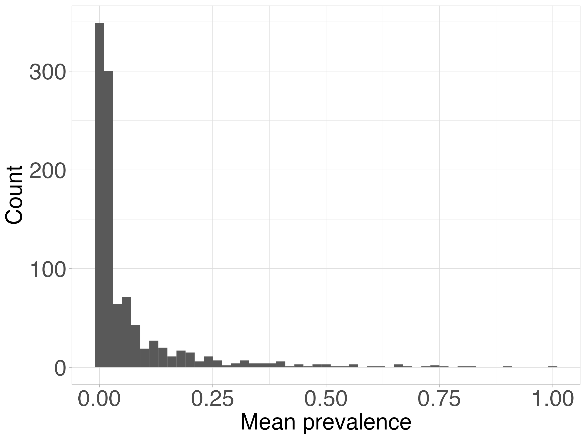
Figure 1: Empirical species occurrence probabilities for fungi data in a Finnish study.

To motivate directions forward in addressing these problems, consider the multivariate probit model (MVP) (Chib and Greenberg, 1998) with covariate effects (initially) removed from consideration for simplicity in exposition:

$$y_{ij} = \mathds{1}(z_{ij}>0),\quad\bm{z}_{i}=(z_{i1},\ldots,z_{ip})^{\top}$$

$$\bm{z}_{i} = \bm{\beta}+\bm{\varepsilon}_{i},\quad\bm{\varepsilon}_{i}\sim N_{p}(\bm{0},\bm{\Sigma}),$$ (1)

with $\bm{\beta}=(\beta_{1},\ldots,\beta_{p})^{\top}=\mbox{E}(\bm{z}_{i})$, $\bm{\Sigma}$ a correlation matrix and $\mathds{1}(\cdot)$ the indicator function. Under this model, the marginal probability of occurrence of species $j$ is $\pi_{j}=\Phi(\mu_{j})$, with $\Phi(\cdot)$ the standard normal cumulative distribution function. Dependence in co-occurrence between species $j$ and $j^{\prime}$ is captured by $\mbox{cor}(z_{ij},z_{ij^{\prime}})=\sigma_{jj^{\prime}}$, the $j,j^{\prime}$ element of matrix $\bm{\Sigma}$. For a recent article developing Bayesian methods for inference in the MVP model allowing for massive $p$, refer to Chakraborty et al. (2023).

In implementing Bayesian analyses of fungi biodiversity data using model (1), there are fundamental problems. The foremost is, as described above, we cannot tie down the identities of the different binary outcomes (species) $j=1,\ldots,p$ in advance. Indeed, we expect to regularly discover new species as we collect additional samples, so that the total numbers of species in $n$ samples may be substantially less than that in $n+m$ samples. Hence, we need a mechanism to allow a growing number of binary outcomes. This is exactly the problem addressed by the IBP, which gives a probability model that concretely allows one to discover new binary features as one collects additional samples. However, the IBP does not characterize within-sample dependence in species occurrences. Potentially, we could use model (1) setting $p$ to a large number with a buffer incorporated to allow new species to be added as the sample size increases. However, simply adding a buffer without careful consideration is ad hoc and may have unanticipated negative consequences. In addition, we face substantial statistical and computational challenges in inferring the elements of the immense correlation matrix $\bm{\Sigma}$. We need some way to borrow information across species in order to accommodate rare species.

Motivated by the above considerations, the focus of this article is on developing a general new framework that bridges between multivariate probit models and IBPs; we refer to this framework as the multivariate probit Indian buffet process (MVP-IBP). We start with a probit version of the IBP that assumes independence across features by letting $\bm{\Sigma}=\bm{I}$; we refer to our model in this special case as the probit IBP (PIBP). We show that the PIBP maintains essentially all of the desirable properties of the traditional IBP. In addition, many of these properties generalize to the case of an arbitrary correlation matrix $\bm{\Sigma}$. In ecological applications, additional information about sites, such as habitat characteristics and spatial or temporal details, is frequently collected. We present an extension of our initial MVP-IBP model to incorporate covariate effects within a regression framework later in the article.

A key challenging in conducting inference in MVP-IBP models is inferring a correlation matrix $\bm{\Sigma}$ that grows in dimension with the number of features. This is both a statistical challenge due to the presence of many rare features and a computational challenge due to the need to conduct posterior inferences for a massive dimensional parameter. We propose a variety of statistical models to reduce dimensionality: (i) assume a single common correlation coefficient between features: $\sigma_{jj^{\prime}}=\rho$; (ii) borrow information across the $\sigma_{jj^{\prime}}$s through a hierarchical model; (iii) borrow information and reduce effective dimensionality through a hierarchical factor model. In models (i)-(ii) we can build on computational developments in Chakraborty et al. (2023) to obtain efficient scalability to massive $p$, while in (iii) we rely on data augmentation Markov chain Monte Carlo algorithms that can scale to $p\approx 1,000$ (e.g., R code implemented on a laptop can be run in hours at that dimension).

As for other IBP-type models, the MVP-IBP framework can be used to predict the number of new features (species) present if one collects an additional $m$ samples after an initial $n$ samples. Such predictions are of substantial interest in biodiversity monitoring applications. We note that there is a substantial ongoing literature on generalizations of the classical IBP model to allow additional flexibility; refer, for example, to Broderick et al. (2013); Di Benedetto et al. (2020); Camerlenghi et al. (2023). Our article adds to this literature but in the fundamentally different direction of targeting dependence within samples in feature occurrence. We also note that, although we are concretely motivated by biodiversity applications, there are direct applications of the MVP-IBP to many other areas ranging from microbiome data (Zhao et al., 2021) to studies of genetics variants (Lee et al., 2010).

2 Dependent infinite latent feature models

2.1 Indian Buffet Process Background

In this section we review key concepts about the Indian buffet process (Griffiths and Ghahramani, 2011) that will be used throughout the paper along with defining notation. Let $\bm{Y}$ be a binary feature matrix, with $n$ rows and an unbounded number of columns, where $y_{ij}=1$ indicates the possession of feature $j$ by object $i$. We let $\mathrm{IBP}(\alpha)$ denote the IBP with parameter $\alpha\in\mathbb{R}^{+}$. In the Indian buffet methapor, rows of $\bm{Y}$ correspond to customers and columns to dishes and the matrix $\bm{Y}$ is sampled as a sequential process. The first customer enters the restaurant and samples the first Poisson$(\alpha)$ number of dishes. After the first customer, the $i$th customer samples each previously sampled dish $j$ with probability $m_{j}/i$, where $m_{j}$ is the number of customers who have previously sampled dish $j$, while also choosing $\mathrm{Poisson}(\alpha/i)$ new dishes. The dishes taken by each customer can be encoded in a binary feature allocation matrix $\bm{Y}$. Customers will tend to choose popular dishes and the number of new dishes will diminish as more customers enter the restaurant. Hence, as $n$ increases $\bm{Y}$ gets sparser.

The IBP can equivalently be derived as the infinite limit of a beta-Bernoulli model. We start by considering the case of models with a finite number $p$ of features, such that $\bm{Y}$ is a binary $n\times p$ feature matrix. Then, we take the conditional distributions

$$\pi_{j}\sim\mathrm{Beta}(\alpha/p,1),\quad\quad y_{ij}\mid\pi_{j}\sim\mathrm{Bernoulli}(\pi_{j}),\quad i=1,\dots,n,\ j=1,\dots,p,$$ (2)

where the $\pi_{j}$ are generated independently and each $y_{ij}$ is independent of all other assignments conditioned on $\pi_{j}$. Griffiths and Ghahramani (2011) show that the likelihood of $\bm{Y}$ generated by the beta-Bernoulli process in the limit that $p$ tends to infinity is equivalent to the one generated by the Indian Buffet Process.

The IBP has several desirable properties that motivate its wide use and provide a simple interpretation. First, under the assumption that the rows of $\bm{Y}$ are exchangeable, the number of features possessed by each object follows a Poisson($\alpha$) distribution. Hence, $\bm{Y}$ is expected to have a finite number of non-zero entries and specifically the expected number of sampled features per customer is $\alpha$. In addition, the number of non empty columns $p^{*}$ is distributed as Poisson($\alpha H_{n}$), where $H_{n}$ is the $n$th harmonic number, $H_{n}=\sum_{i=1}^{n}1/i$. This is easily shown using the fact that the number of new columns generated by the $i$th customer is Poisson($\alpha/i$), with the total number of columns being the sum of these quantities.

2.2 Model specification

We introduce the multivariate probit Indian buffet process (MVP-IBP). As in the IBP setting, we derive a distribution on infinite binary matrices by starting with a truncation level $p$ for the number of features and then taking the limit as $p\rightarrow\infty$.

Similarly to the multivariate probit, the MVP-IBP model is defined through a latent Gaussian construction. Let ${\bm{z}_{i}=(z_{i1},\dots,z_{ip})^{\top}\in\mathds{R}^{p}}$ denote a $p$-variate latent continuous variable for $i=1,\dots,n$ and let $y_{ij}$ be 1 or 0 according to the sign of $z_{ij}$. The proposed MVP-IBP model is

$$y_{ij}=\mathds{1}(z_{ij}>0),\quad z_{ij}=\beta_{j}+\varepsilon_{ij},\quad\beta_{j}\sim N(\mu_{p},\tau_{p}^{2}),\quad\bm{\varepsilon}_{i}=(\varepsilon_{i1},\dots,\varepsilon_{ip})^{\top}\sim N_{p}(\bm{0},\bm{\Sigma}),$$ (3)

where $\bm{\beta}=(\beta_{1},\dots,\beta_{p})^{\top}$ is a $p$-dimensional vector of coefficients controlling the marginal dish selection (species occurrence) probabilities and $\bm{\Sigma}$ is a $p\times p$ positive definite correlation matrix controlling dependence in dish selection (species presence). Let $\sigma_{jj^{\prime}}$ denote the $j,j^{\prime}$ element of matrix $\bm{\Sigma}$. We assume independence across samples $i=1,\ldots,n$; extensions to accommodate covariates and spatio-temporal dependence are straightforward. We present an extension of MVP-IBP to include covariates in Section 5.1. Marginally, $y_{ij}\sim\mbox{Bernoulli}(\pi_{j})$ with

$$\mathrm{pr}(y_{ij}=1\mid\beta_{j})=\pi_{j}=\Phi(\beta_{j}),$$ (4)

for $j=1,\dots,p$ and $i=1,\dots,n$. The hierarchical prior on $\beta_{j}$ in (3) enables borrowing of information across dishes (species), which is critical in analyzing data containing rare species.

Hence, the MVP-IBP model corresponds to a probit-Bernoulli process having a construction similar to the IBP defined in (2). Specifically, both approaches generate dishes (species) from a Bernoulli process, with the IBP drawing the occurrence probabilities from a beta distribution, while the MVP-IBP draws these probabilities from a probit process. We will show that the MVP-IBP can closely mimic the IBP when $\bm{\Sigma}=\bm{I}$, a special case we refer to as the probit IBP (PIBP). However, the MVP-IBP has the additional flexibility of allowing dependence in dish selection (species occurrennce), with $\sigma_{jj^{\prime}}$ controlling the dependence between $y_{ij}$ and $y_{ij^{\prime}}$.

The hyperparameters $\mu_{p}$ and $\tau_{p}$ in the prior for $\beta_{j}$ play a crucial role in determining the induced likelihood of $\bm{z}_{i}$ and thus also the likelihood of $\bm{Y}$. Specifically, they control the number of features (species) within each sample and the rate of growth of non-zero columns (total number of species across the samples). We will show in the next section that the default values

$$\mu_{p}=\sqrt{1+\tau_{p}^{2}}\,\Phi^{-1}\left(\frac{\alpha}{\alpha+p}\right),\quad\tau_{p}=\sqrt{2\log p},\quad\alpha\in\mathbb{R}^{+}$$ (5)

lead to preservation of many of the desirable properties of the IBP. We show that $\alpha$ plays a similar role to the IBP parameter in controlling the expected number of features per sample.

Similarly to the usual finite MVP model, the likelihood of $\bm{Y}$ under the MVP-IBP is not available analytically in involving an integral over a multivariate normal distribution. However, there is a rich literature on efficient posterior computation algorithms for finite MVP models (Chakraborty et al., 2023), which we will leverage on for MVP-IBP inference. In the next subsection we show several appealing theoretical properties providing support for the MVP-IBP model. For example, we will prove that the limiting number of non-zero entries in $\bm{Y}$ as $p\rightarrow\infty$ is almost surely finite. This ensures that the number of sampled features (species) will be finite even in the limiting case.

2.3 General properties

In this section we present some theoretical properties motivating the MVP-IBP model described in (3) and (5). Besides the general results, we will also focus on the PIBP model, the special case with $\bm{\Sigma}=\bm{I}$. Proofs are given in the supplementary materials.

First, we prove that in the limiting case the expected number of non-zero entries is finite. More specifically, Theorem 1 shows that the MVP-IBP has the same number of expected features as the IBP, preserving an easy and intuitive interpretation for the parameter $\alpha$. It also shows that for the PIBP model the number of features per sample has the same distribution as the IBP.

Theorem 1.

Consider the MVP-IBP model and let $n_{i}=\sum_{j=1}^{p}y_{ij}$. Then $\lim_{p\to\infty}E(n_{i})=\alpha,$ for each $i=1,\dots,n$. If we further assume $\bm{\Sigma}=\bm{I}$, then $n_{i}\sim Po(\alpha)$ for $p\to\infty$.

Theorem 1 ensures that the number of sampled features is finite, so that $\mathrm{pr}(n_{i}<\infty)=1$. Then, since the objects are independent, it easily follows that the expected total number of non-zero entries is $n\alpha$. In the following proposition we also characterize the limiting variance of the number of features per object. In the PIBP and IBP models the limiting variance of $n_{i}$ is $\alpha$, given that $n_{i}$ follows a Poisson distribution as $p\to\infty$.

Proposition 1.

Consider the MVP-IBP model and assume that $\sigma_{jj^{\prime}}\in\{\rho_{1},\ldots,\rho_{k}\}$ with $k\in\mathds{N}$. Then $\alpha+\alpha^{2}/2\,(\underset{k}{\mathrm{min}}\,|\exp\{\rho_{k}\}-1|)\leq\lim_{p\to\infty}\mathrm{var}(n_{i})\leq\alpha+\alpha^{2}/2\,(\underset{k}{\mathrm{max}}\,|\exp\{\rho_{k}\}-1|)$, for each $i=1,\dots,n$.

Proposition 1 provides bounds for the limiting variance of the numbers of features per object. When the species are highly correlated the upper bound is larger, enabling more variability in the number of species sampled for each site. Instead, if the correlations among species are close to zero the bounds are very narrow and the variance of $n_{i}$ tends to $\alpha$. Hence, the variance of the number of species per site is always greater than $\alpha$ and may increase to encompass the dependence among species. The assumption we made in Proposition 1 about a finite number of correlation coefficients is consistent with the way we parametrize the correlation matrix to reduce dimensionality. This assumption is trivially satisfied in the common correlation coefficient case, while the more flexible approaches we propose use shrinkage to reduce effective dimensionality.

Another property the MVP-IBP preserves from the IBP is sparsity: as $p$ grows the feature matrix gets sparser while allowing the possibility of sampling new features. This characteristic reflects the expected behaviour of the species sampling matrix, where many species are rare and have a tiny probability a priori of being observed. We define a sparsity property of the MVP-IBP in the following proposition.

Proposition 2.

The matrix sampled under the MVP-IBP model is sparse, i.e. $\lim_{p\to\infty}\mathrm{pr}(y_{ij}=1)=\lim_{p\to\infty}\frac{\alpha/p}{\alpha/p+1}=0$ holds for each $i=1,\dots,n$.

Proposition 2 shows that the marginal probabilities go to zero at a linear rate as $p$ grows; this same property holds for the IBP. This property implies that the binary latent feature matrix is sparse.

As in our motivating applications there are some common species and many very rare species, it is important to characterize the expected number of common features corresponding to the most popular dishes in the Indian buffet metaphor. Common features are in the right tail of the distribution of the $\pi_{j}$s across $j$. In insect and fungi ecology, there are many very rare species having $\pi_{j}\approx 0$ with some common species having $\pi_{j}>\epsilon.$ In order to be realistic for our motivating applications, we need the MVP-IBP to allow a proportion of common species instead of forcing all the $\pi_{j}$s to be close to zero as $p\to\infty$. In definition 1 we formalize the notion of common features.

Definition 1.

Let $\bm{Y}$ be an $n\times p$ binary feature allocation matrix ($i=1,\dots,n$, $j=1,\dots,p$) and let $\pi_{j}$ denote the marginal probability of sampling feature $j$ for $i=1,\dots,n$. The feature $j$ is a common feature if the probability of generating that feature is higher than a fixed threshold $\epsilon$, i.e. $\mathrm{pr}(\pi_{j}>\epsilon)$.

Let $c_{j}^{(\epsilon)}=\mathds{1}(\pi_{j}>\epsilon)$, $j=1,\dots,p$, denote the binary variables that identify the common features and let $c^{(\epsilon)}=\sum_{j=1}^{p}c_{j}^{(\epsilon)}$ denote the total number of common features for threshold $\epsilon$. For the IBP model the expected total number of common features is

$$E(c^{(\epsilon)})=\sum_{j=1}^{p}Pr(\pi_{j}>\epsilon)=p(1-B_{\epsilon}(\alpha/p,1))=p(1-\epsilon^{\alpha/p})\xrightarrow[p\to\infty]{}-\alpha\log\epsilon,$$

where $B_{x}(a,b)$ is the regularized incomplete beta function. The following proposition states a related result for the MVP-IBP model.

Proposition 3.

For the MVP-IBP model the expected total number of common features is

$$\lim_{p\to\infty}E(c^{(\epsilon)})=\alpha\exp\left\{-\Phi^{-1}(\epsilon)-\frac{1}{2}\right\}.$$

Hence, the expected number of common species under the MVP-IBP differs somewhat from that for the IBP. However, the functional relationship with the commonness threshold $\epsilon$ is similar, as illustrated in Figure 2. This figure also compares the expected number of common species under the MVP-IBP and IBP models with the empirical count observed in our motivating data. For this plot we utilized an optimized value of $\alpha$, set to 70. Notably, the theoretical curves for the MVP-IBP and IBP models align closely, indicating that both models exhibit comparable behavior. Moreover, they effectively capture the observed total number of common species in the fungi co-occurrence data.

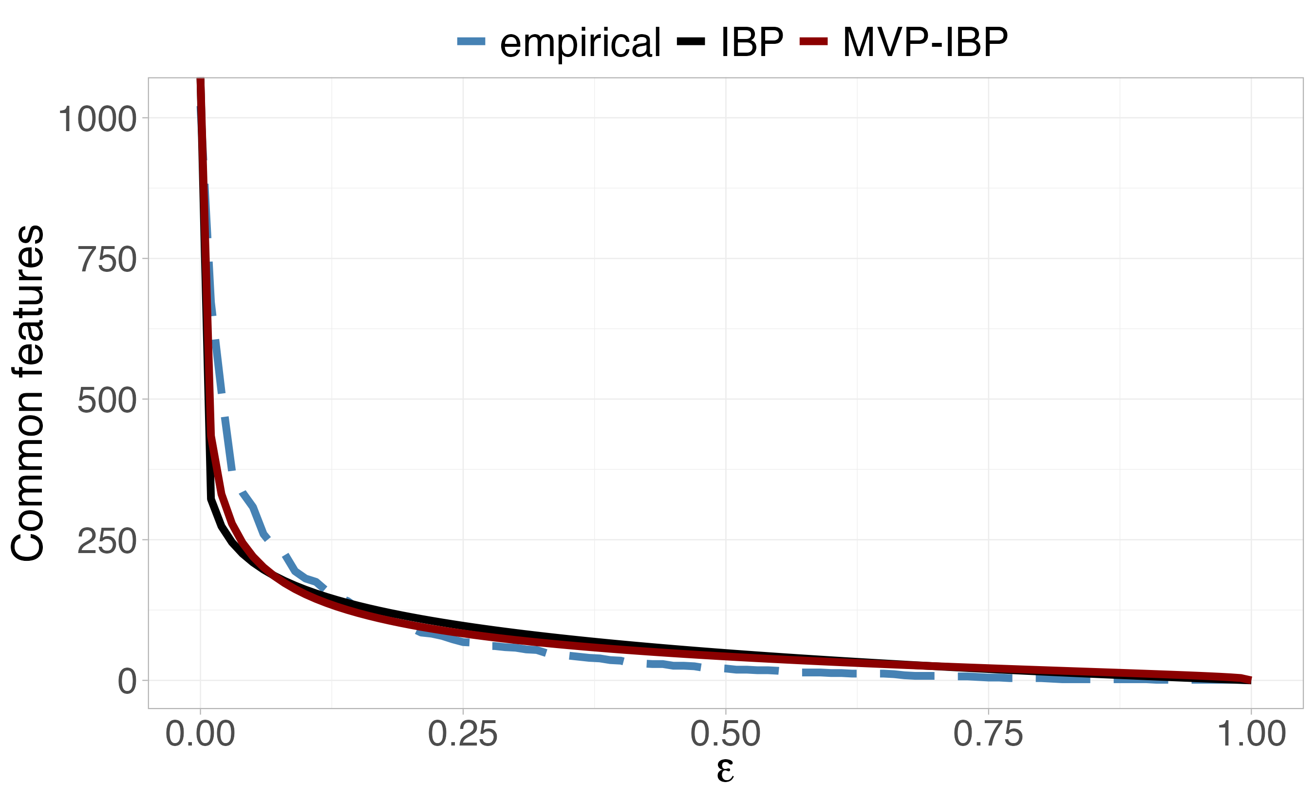
Figure 2: Expected total number of common features for the MVP-IBP (red line) and IBP (black line) models for different values of $\epsilon$, with $\alpha=70$. The dashed blue line shows the empirical number of common species for a grid of values of $\epsilon$ for the fungi co-occurence data.

An additional desirable property is to characterize the number of non empty columns $p^{*}$, i.e. the effective dimension of the sampled matrix. In ecological applications, this corresponds to the species richness measure of biodiversity. More precisely, let $p^{*}$ denote the number of features for which $n_{j}=\sum_{i=1}^{n}y_{ij}>0$. Griffiths and Ghahramani (2011) showed that the expected value of $p^{*}$ for the IBP is $\alpha H_{n}$ and thus the number of nonzero columns grows as $\mathcal{O}(\alpha\log n)$. Theorem 2 shows that the growth rate for the MVP-IBP model is the same, while providing further insights into the expected value and distribution of $p^{*}$ in the PIBP case.

Theorem 2.

Consider the MVP-IBP model and let $w_{j}=\mathds{1}(n_{j}>0)$ and $p^{*}=\sum_{j=1}^{p}w_{j}$. Then for $p\to\infty$ we have:

1. $p^{*}$ grows as $\mathcal{O}(\alpha\log n);$

2. $\alpha(H_{n}-a)<E(p^{*})<\alpha(H_{n}-b)$, with $a=0.073$ and $b=0.02$.

If we further assume $\bm{\Sigma}=\bm{I}$, then $p^{*}\sim\mbox{Poisson}(l)$ with $(H_{n}-a)<l<(H_{n}-b)$ for $p\to\infty$.

3 Correlation structure modeling and posterior computation

The MVP-IBP model described in (3) and (5) provides a general framework that can be used in different settings under appropriate choices of the correlation matrix. Here, we propose alternative approaches to model $\bm{\Sigma}$ for reducing dimensionality and overcoming the inferential challenges of rare species (features). Specifically, in Section 3.1 we describe an approach building on recent computational developments for Bayesian inference on high-dimensional multivariate binary data (Chakraborty et al., 2023), while in Section 3.2 we propose an approach based on factor models.

In both methods, posterior inference is conducted by truncating the number of species at a suitably large value $P$, which is substantially greater than the observed number of species $p$. Truncation is standard practice in nonparametric Bayesian models involving infinitely-many components, ranging from mixture models (Ishwaran and James, 2001) to latent feature models (Williamson et al., 2010; Doshi et al., 2009). In the Supplementary Materials, we provide simulation results showing that posterior inferences for the MVP-IBP model are robust with respect to the choice of truncation level.

3.1 Posterior computation via two-stage inference

To facilitate scaling to large numbers of species, one possibility is to adapt a recently proposed algorithm for rapid posterior computation in MVP models (Chakraborty et al., 2023). This algorithm focuses on approximating marginal posterior distributions for the parameters, obtaining accurate point estimation and uncertainty quantification. We first obtain approximations $\Pi_{j}^{*}(\beta_{j}\mid y)$ for the marginal posteriors of the random intercepts $\beta_{j}$ for $j=1,\dots,P$; we use a simplified likelihood that replaces $\bm{\Sigma}$ with the identity matrix and apply Laplace approximations. Let $l_{j}(\beta_{j})$ denote the log-likelihood of the $j$th binary outcome under this simplified model and $\Pi_{j}(\beta_{j})$ denote the prior distribution $\beta_{j}\sim N(\mu_{P},\tau_{P}^{2})$. Then $\Pi_{j}^{*}(\beta_{j}\mid y)\approx N(\hat{\beta}_{j},\bm{Q}_{j})$, where $\hat{\beta}_{j}=\mathrm{argmax}_{\beta_{j}}\{l_{j}(\beta_{j})+\log\Pi_{j}(\beta_{j})\}$ and $\bm{Q}_{j}$ is the corresponding inverse Hessian. Chakraborty et al. (2023) showed in their Theorem 3.5 that $\Pi_{j}^{*}(\beta_{j}\mid y)$ is asymptotically normal centered at a maximum composite likelihood estimator with the appropriate variance.

We then proceed with obtaining approximations to the marginal posterior distributions of the elements of the correlation matrix $\bm{\Sigma}$. Let $\Pi_{\Sigma}(\cdot)$ denote the prior for the correlation matrix $\bm{\Sigma}$. We approximate the marginal posterior distributions of $\sigma_{jj^{\prime}}$ by considering a bivariate probit model between the pairs $(j,j^{\prime})$. We combine this likelihood with the marginal prior for $\sigma_{jj^{\prime}}$ to obtain a Gaussian approximation $\Pi^{*}_{jj^{\prime}}(\sigma_{jj^{\prime}}\mid y)$ for the posterior of $\sigma_{jj^{\prime}}$, as justified in Theorem 3.7 of Chakraborty et al. (2023). The mean $\hat{\sigma}_{jj^{\prime}}$ and the variance $s_{jj^{\prime}}^{2}$ of the approximate posteriors for $\sigma_{jj^{\prime}}$ are obtained using Gauss-Legendre quadrature. Chakraborty et al. (2023) show that asymptotically the distribution is centered at the maximum composite likelihood estimator from the bivariate margins. Predictions can be obtained using pairwise approximations to the posterior predictive.

We consider two different models for the correlation matrix $\bm{\Sigma}$. The first assumes a common correlation coefficient for all pairs of species, $\rho_{jj^{\prime}}=\rho$. We induce a prior for $\rho$ by letting $\zeta=0.5\log[(1+\rho)/(1-\rho)]$ with $\zeta\sim N(0,w_{0}^{2})$. We use Metropolis-Hastings to sample from the conditional posterior of $\rho$ given the $\beta_{j}$s; for this simple choice of correlation structure, we do not use the above asymptotic Gaussian approximation for the posterior of $\sigma_{jj^{\prime}}$. As a more flexible alternative, we also consider a hierarchical model that lets

$$\zeta_{jj^{\prime}}=0.5\log[(1+\sigma_{jj^{\prime}})/(1-\sigma_{jj^{\prime}})]\sim N(0,\omega^{2}),\quad\omega^{2}\sim IG(a_{\omega},b_{\omega}),$$ (6)

where $IG(a,b)$ is an inverse-gamma distribution. This hierarchical model shrinks the correlation coefficients towards zero; such shrinkage is particularly important for rare species. Chakraborty et al. (2023) propose a similar approach and show excellent practical performance, while noting that (6) does not arise as the marginal of a prior for $\bm{\Sigma}$. To complete a Bayesian specification of the MVP-IBP model, we choose $\alpha\sim Ga(a_{\alpha},b_{\alpha})$. Algorithm 1 of the supplementary materials describes an extension of the algorithm in Chakraborty et al. (2023) to allow empirical Bayes estimation of $\alpha$ and $\omega$.

3.2 MVP-IBP factor model

The following MVP-IBP factor model is an important special case of the general MVP-IBP framework described in Section 2.2, which enables dimensionality reduction in modeling the correlation matrix:

$$y_{ij}=1(z_{ij}>0),\quad z_{ij}=\beta_{j}+\bm{\lambda}_{j}^{T}\bm{\eta}_{i}+\varepsilon_{ij},\quad\varepsilon_{ij}\sim N(0,1),$$ (7)

where $\bm{\eta}_{i}\sim N_{K}(\bm{0},\bm{I})$ is a $k\times 1$ vector of latent factors and $\bm{\lambda}_{j}^{\top}=(\lambda_{j1},\dots,\lambda_{jk})$ denotes the $j$th row of $\bm{\Lambda}$, a $P\times k$ matrix of factor loadings ($k<P$), for $j=1,\dots,p$ and $i=1\dots,n$. Dependence is induced by marginalizing out the factors to obtain $\bm{z}_{i}\mid\bm{\beta},\bm{\Lambda}\sim N(\bm{\beta},\bm{\Omega})$, where $\bm{\Omega}=\bm{\Lambda}\bm{\Lambda}^{\top}+\bm{I}$. To obtain an MVP-IBP formulation, we rescale the latent variables $z_{ij}$, dividing them by $(1+\bm{\lambda}_{j}^{\top}\bm{\lambda}_{j})^{1/2}$ for each $i=1,\dots,n$ and $j=1,\dots,P$. Inference focuses on the scaled coefficients $\tilde{\beta_{j}}=\beta_{j}/\ (1+\bm{\lambda}_{j}^{\top}\bm{\lambda}_{j})^{1/2}$, for which we choose normal priors $\tilde{\beta_{j}}\sim N(\mu_{P},\tau_{P}^{2})$. We let $\tilde{\bm{\beta}}=(\tilde{\beta}_{1},\dots,\tilde{\beta}_{P})^{\top}$ denote the vector of scaled coefficients. The MVP-IBP factor model can equivalently be written as

$$y_{ij}=1(z_{ij}>0),\quad\bm{z}_{i}=\tilde{\bm{\beta}}+\varepsilon_{i},\quad\varepsilon_{i}\sim N(\bm{0},\bm{\Sigma}),\quad\tilde{\beta}_{j}\sim N(\mu_{P},\sigma_{P}^{2}),$$ (8)

where $\bm{\Sigma}=\bm{D}^{-1}(\bm{\Lambda}\bm{\Lambda}^{\top}+\bm{I}_{P})\bm{D}^{-1}$ with $\bm{D}=\operatorname{diag}(\sqrt{1+\bm{\lambda}_{1}^{\top}\bm{\lambda}_{1}},\dots,\sqrt{1+\bm{\lambda}_{P}^{\top}\bm{\lambda}_{P}})$. Equation (8) is a special case of the multivariate probit Indian buffet process defined in (3) and (5).

To select the number of factors $k$, we rely on shrinkage priors for the factor loadings matrix (Bhattacharya and Dunson, 2011). Specifically, we use the cumulative shrinkage process prior (CUSP) of Legramanti et al. (2020). We choose $\lambda_{jk}\mid\theta_{k}\sim N(0,\theta_{k})$ (for $j=1,\dots,P$ and $k\in\mathds{N}_{+}$) and let

$$\theta_{k}\mid\pi_{k}\sim(1-\pi_{k})IG(a_{\theta},b_{\theta})+\pi_{k}\epsilon_{\theta_{\infty}},\quad\pi_{k}=\sum_{l=1}^{k}\omega_{l},\quad\omega_{l}=\nu_{l}\prod_{m=1}^{l-1}(1-\nu_{m}),$$ (9)

where $\nu_{k}$ are independent $Beta(1,\kappa)$ variables. The entries of the loading matrix are increasingly shrunk towards zero as the column index increases, leading to effective deletion of unnecessary factors when $\theta_{\infty}\approx 0$. CUSP can be efficiently implemented through an adaptive MCMC algorithm setting an upper bound of $K$ on the number of factors, as justified in Legramanti et al. (2020).

Posterior inference for the MVP-IBP factor model truncated at $P$ species proceeds via a Gibbs sampler. This sampler relies on data augmentation which exploits the latent variable construction of the probit model. Within this sampler, we update the key $\alpha$ parameter assuming a gamma prior, $\alpha\sim Ga(a_{\alpha},b_{\alpha})$. The detailed steps of sampler are given in Section S.2 of the supplementary materials.

4 Performance assessments in simulations

We evaluate the performance of the factor and two-stage inference versions of the proposed method through simulation studies. The target of the simulation study is to assess the accuracy of estimating the true marginal occurrence probabilities $\pi_{j}^{*}=\Phi(\beta_{j}^{*})$ and the true associated correlation structure $\bm{\Sigma}^{*}$. In addition, in ecological applications there is substantial interest in predicting the number of new species that would be discovered if $m$ additional samples were collected; we assess the performance of such predictions. For predictive assessments, we introduce notation making explicit the dependence of the number of observed species on the sample size. In particular, let $p^{*}_{n}$ denote the sample species richness, i.e. the number of observed species in $n$ samples. Then, the focus is to predict conditionally on $p^{*}_{n}$ the number of new species discovered in an additional $m$ samples, i.e. $\Delta_{m}=p^{*}_{n+m}-p^{*}_{n}$. We compare the results under different versions of MVP-IBP with the IBP and the bigMVP method of Chakraborty et al. (2023). Inference in the IBP model proceeds through a Gibbs sampler, considering a gamma prior for $\alpha$ and following the truncated beta-binomial representation of Griffiths and Ghahramani (2011). For the bigMVP method we consider the hierarchical version (bigMVPh) of Chakraborty et al. (2023), suitable when dealing with rare outcomes.

To simulate the data we consider a fixed sample size of $n=80$ and vary the number of observed species $p^{*}_{n}$, which is upper bounded by $P=300$. The parameter $\alpha$ is varied, ranging from 2 to 40 in increments of two, obtaining 20 different simulated datasets. The different values of $\alpha$ lead to different numbers of observed species. As outlined in Section 2.3, $p^{*}_{n}$ grows as $\mathcal{O}(\alpha\log n)$, so with a constant sample size, a higher $\alpha$ results in a larger number of species sampled. For each value of $\alpha$, we consider three data-generating scenarios: 1) (factor) the data are simulated under the factor MVP-IBP model, 2) (tobit) the data are generated under a misspecified factor MVP-IBP model where the underlying continuous data $z_{ij}$ are generated as $\bm{z}_{i}\sim t_{10}(\bm{\beta}^{*},\bm{\Sigma}^{*})$, where $t_{10}(\bm{\beta}^{*},\bm{\Sigma}^{*})$ denotes a multivariate $t$ distribution with $10$ degrees of freedom with mean $\bm{\beta}^{*}$ and scale matrix $\bm{\Sigma}^{*}$ and 3) (common) the data are simulated under the MVP-IBP model where $\bm{\Sigma}^{*}=\rho\mathbf{1}_{P}\mathbf{1}^{\top}_{P}+(1-\rho)\bm{I}_{P}$ with $\mathbf{1}_{P}$ a $P$-dimensional vector of all ones and $\rho$ drawn from a uniform distribution in $[0,0.8]$. The latter scenario includes cases where $\bm{\Sigma}=\bm{I}_{P}$ and this data-generating setting closely resembles the IBP model construction, as detailed in Section 2.3.

In estimating the IBP and MVP-IBP models, we set the parameters for the gamma prior on $\alpha$ such that the distribution is centered on the empirical mean of the number of features per sample. The Gibbs samplers for the factor MVP-IBP and the IBP are run for 2000 iterations after a burn-in of 500. Following Chakraborty et al. (2023), the initial conditional sampler for the two-stage inference method is run 200 times with the first 50 samples discarded.

We start by comparing performance of the IBP and factor MVP-IBP in estimating the true marginal occurrence probability $\bm{\pi}^{*}=(\pi_{1}^{*},\dots,\pi_{P}^{*})^{\top}$ and correlation matrix $\bm{\Sigma}^{*}$ through a Monte Carlo estimate of the posterior averaged mean square error (MSE). For each of the 20 simulations in each scenario, we compute $\sum_{j=1}^{P}E[(\pi_{j}-\pi_{j}^{*})^{2}\mid y]/P$ and $\sum_{j=1}^{P}\sum_{q=1}^{P}E[(\Sigma_{jq}-\Sigma_{jq}^{*})^{2}\mid y]/P^{2}$. To assess the performance of the models in predicting the number of new species if additional samples are collected, we focus on predicting the number of new species in the last 10 samples. Hence, the key quantity is $\Delta_{10}^{*}=p^{*}_{50}-p_{40}^{*}$. By observing that $E[p_{n}^{*}]=\sum_{j=1}^{P}w_{j}$ with $w_{j}\sim\textrm{Bernoulli}(1-(1-\pi_{j})^{n})$, it follows that $E[p^{*}_{n}]=\sum_{j=1}^{P}(1-(1-\pi_{j})^{n})$. Let $\hat{p}^{(b)}_{50}=\sum_{j=1}^{P}(1-(1-\pi_{j}^{(b)})^{50})$, where $\pi_{j}^{(b)}$ are the posterior samples of $\pi_{j}$ for $b=1,\dots,B$ with $B$ the total number of posterior draws. Then, we can easily obtain $\hat{\Delta}_{10}^{(b)}=\hat{p}^{(b)}_{50}-p^{*}_{40}$ for each sample. Analogously, let $p_{50}^{*}=\sum_{j=1}^{P}(1-(1-\pi_{j}^{*})^{50})$. Then, for each of the 20 synthetic datasets in each scenario we compute the Monte Carlo estimate of $E[(\hat{\Delta}_{10}-\Delta_{10}^{*})^{2}\mid y]$ for the IBP and factor MVP-IBP models, i.e. $\sum_{b=1}^{B}(\hat{\Delta}_{10}^{(b)}-\Delta_{10}^{*})^{2}/B$. The results are shown in the top panel of Figure 3. In the factor and tobit scenarios, the factor MVP-IBP outperforms the IBP across all evaluated metrics, while in the common scenario the IBP performs better in terms of $\bm{\pi}^{*}$ and $\Delta^{*}_{10}$. This is as expected since in this scenario correlation is zero, which matches the IBP assumption.

Subsequently, we compare the approximate samplers, the hierarchical version of MVP-IBP (MVP-IBPh) and the bigMVPh of Chakraborty et al. (2023), by evaluating the estimation errors of $\pi_{j}^{*}$, $\Delta_{10}^{*}$ and $\bm{\Sigma}^{*}$. We compute the estimation errors for the marginal occurrence probabilities as $\|\hat{\bm{\pi}}-\bm{\pi}^{*}\|/P$ for any estimator $\hat{\bm{\pi}}$, where $\|\cdot\|$ denotes the Frobenius norm. For both competing methods we consider as estimators the posterior means. We considered the same Frobenius errors for evaluating the model’s performance in terms of $\Delta^{*}_{10}$ and $\bm{\Sigma}^{*}$. The bottom panel of Figure 3 shows the results for the 20 simulations in each scenario. Across all scenarios, the MVP-IBP model consistently performs better than bigMVP for estimating the marginal occurrence probabilities and the correlation matrix and predicting the number of new species.

Figure S2 of the supplementary materials shows that the results for the factor MVP-IBP and hierarchical MVP-IBP are robust to changes in the truncation level. Code to implement the MVP-IBP method and to replicate our analysis is available at https://github.com/federicastolf/MVP-IBP.

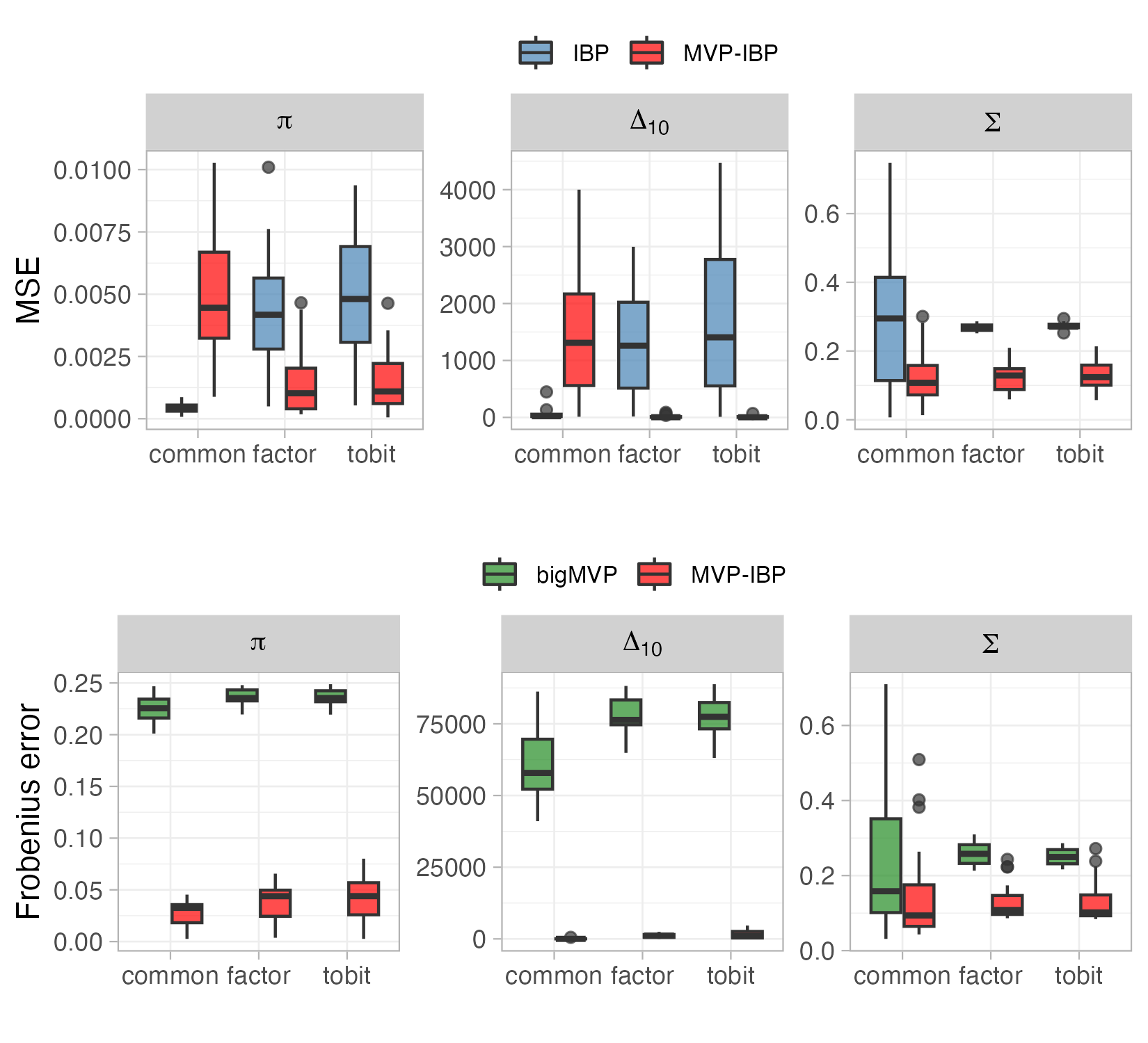
Figure 3: The top panel shows the performance in terms of mean square error for $\bm{\pi}^{*}$, $\bm{\Sigma}^{*}$ and $\Delta_{10}^{*}$ of the factor MVP-IBP and the IBP in 20 simulations for each scenario. The bottom panel shows the performance in terms of Frobenius error for $\bm{\pi}^{*}$, $\bm{\Sigma}^{*}$ and $\Delta_{10}^{*}$ of the hierarchical MVP-IBP and the bigMVP in 20 simulations for each scenario

5 Fungal biodiversity application

5.1 Extension for regression setting

In this section, we relax the exchangeability assumption among rows and extend the MVP-IBP model to incorporate covariates. This extension is particularly relevant in species sampling data, where additional information about the samples is typically available. This information may include temporal details and habitat characteristics, providing a more comprehensive understanding of the species occurrences. Let $\bm{x}_{i}=(x_{i1},\dots,x_{iq})^{\top}$ be the covariate for each sample $i$ and $\bm{b}_{j}=(b_{j1},\dots,b_{jq})^{\top}$ the regression coefficients specific to species $j$, with $q$ the number of covariates. We define a covariate-dependent MVP-IBP model, an extension of the base MVP-IBP model defined in (3), by assuming

$$y_{ij}=\mathds{1}(z_{ij}>0),\quad z_{ij}=\beta_{j}+\bm{x}_{i}^{\top}\bm{b}_{j}+\varepsilon_{ij},\quad\quad\bm{b}_{j}\sim N_{q}(\bm{\gamma},\bm{\Psi}),\quad\bm{\varepsilon}_{i}\sim N_{p}(\bm{0},\bm{\Sigma}),$$ (10)

where $\beta_{j}\sim N(\mu_{p},\tau_{p}^{2})$ with the same values for $\mu_{p}$ and $\tau_{p}$ of equation (5). We assume independence between the random intercepts and the regression coefficients. Marginally for each of the species we have $\mathrm{pr}(y_{ij}=1\mid\beta_{j},\bm{b}_{j})=\Phi(\beta_{j}+\bm{x}_{i}^{\top}\bm{b}_{j})$.

In the following, we show how the theoretical results presented in Section 2.3 adapt to the covariate-dependent MVP-IBP model. First, we prove that for $p\to\infty$ the expected value and the variance of the number of features per object $n_{i}=\sum_{j=1}^{p}y_{ij}$ are finite. More specifically, Theorem 1 shows that the variance and the expected value of $n_{i}$ preserve the structure of the base MVP-IBP, adjusting for the covariate effects.

Theorem 3.

Consider the covariate-dependent MVP-IBP model and let $g_{i}=\exp\{\bm{x}_{i}^{\top}\bm{\gamma}+\frac{1}{2}(\bm{x}_{i}^{\top}\bm{\Psi}\bm{x}_{i}-1)\}$. Then for $i=1,\dots n$

1. $\lim_{p\to\infty}E(n_{i})=\alpha g_{i}$;

2. if we further assume $\sigma_{jj^{\prime}}\in\{\rho_{1},\ldots,\rho_{k}\}$ with $k\in\mathds{N}$, we have $\alpha g_{i}(1+\frac{1}{2}\alpha g_{i})\,(\underset{k}{\mathrm{min}}\,|\exp\{\rho_{k}\}-1|)\leq\lim_{p\to\infty}\mathrm{var}(n_{i})\leq\alpha g_{i}(1+\frac{1}{2}\alpha g_{i})\,(\underset{k}{\mathrm{max}}\,|\exp\{\rho_{k}\}-1|)$.

Both the variance and the expected value for the number of species for each sample directly depend on $\alpha$ and are adjusted by the covariate values and regression coefficients. The above theorem provides valuable insights into the role of the regression coefficients $\bm{b}_{j}$ and covariates on species richness in ecology, beyond their roles in impacting the individual species occurrence probabilities. From the Theorem, it directly follows that the expected total number of non-zero entries is $\alpha\sum_{i=1}^{n}g_{i}$.

It is straightforward to show that the covariate-dependent MVP-IBP model maintains key sparsity properties, with finitely many observed species in each sample and many of the species being rare. We are also interested in characterizing the behaviour of the expected number of common species. The following proposition formalizes this result.

Proposition 4.

Let $c_{ij}^{(\epsilon)}=\mathds{1}(\Phi(\beta_{j}+\bm{x}_{i}^{\top}\bm{b}_{j})>\epsilon)$ and $c_{i}^{(\epsilon)}=\sum_{j=1}^{p}c_{ij}^{(\epsilon)}$ denote the number of common species with threshold $\epsilon$ for sample $i$. Then, for the covariate-dependent MVP-IBP model, the expected number of common features for sample $i$ is

$$\lim_{p\to\infty}E(c_{i}^{(\epsilon)})=\alpha\exp\Big{\{}-\Phi^{-1}(\epsilon)+\frac{1}{2}(\bm{x}_{i}^{\top}\bm{\Psi}\bm{x}_{i}-1)+\bm{x}_{i}^{\top}\bm{\gamma}\Big{\}},$$

for $i=1,\dots,n$.

This result is the same as for our initial MVP-IBP model, but with an adjustment for the covariate effect. Specifically, the expected number of common species depends on the covariance matrix $\bm{\Psi}$ and the mean vector $\bm{\gamma}$ of the prior for the regression coefficients $\bm{b}_{j}$.

For rare species, there is insufficient information in the data to accurately estimate the species-specific regression coefficients. To address this problem, it is natural to choose a hierarchical structure to borrow information across the different species. Hence, we let

$$\bm{b}_{j}\mid\bm{\gamma},\bm{\Psi}\sim N_{q}(\bm{\gamma},\bm{\Psi}),\quad(\bm{\gamma},\bm{\Psi})\sim\mathrm{NIW}(\bm{\gamma}_{0},\iota,d,\bm{\Xi}),$$ (11)

where $\mathrm{NIW}(\bm{\gamma}_{0},\iota,d,\bm{\Xi})$ is a Normal-Inverse Wishart prior distribution. The algorithms for posterior computation in Section 3 can be easily adapted to accommodate the additional covariates and the hierarchical structure for the regression coefficients. For the factor MVP-IBP, the full conditional distributions are straightforward to obtain, given the conjugacy of the prior distribution for $\bm{b}_{j}$. For the hierarchical MVP-IBP, we deal with the hierarchical structure for $\bm{b}_{j}$ in the same way that we estimate $\alpha$; see Section S.4 of the supplementary materials for more details.

5.2 Fungi co-occurrence data analysis

We analyze data from a fungi biodiversity study in Finland (Abrego et al., 2018). Fungi are a highly diverse group of organisms, they play major roles in ecosystem functioning and are important for human health, food production and nature conservation. Data consist of 134 samples from different sites across four study locations in Finland, with 29 samples in Site 1, 97 samples in Site 2, 2 samples in Site 3 and 6 samples in Site 4. A cyclone sampler was used to acquire spore samples from each study site. Based on a probabilistic molecular species classifier using DNA barcoding, $1021$ distinct species were identified. For each sample, the data include two covariates: a categorical variable with four levels indicating the study location and a continuous variable that provides information about the week. To assess any temporal dependence or effect of habitat type, we include these covariates in the model as predictors. We encode the site variable through three dummies with Site 2 (the one with the highest number of observations) as the reference level. Hence, we considered the regression setting for the MVP-IBP model outlined in Section 5.1 with the number of covariates $q=4$.

Given the massive number of fungal species identified and the presence of many rare species, we analyze the data with the hierarchical formulation of the MVP-IBP model described in Section 3.1. This approach enables information sharing among species and achieves computational efficiency. Similarly to the simulations, we center the distribution of $\alpha$ on the empirical mean of the number of species per sample. For the regression coefficients we use a normal prior centered in zero, i.e. $\bm{b}_{j}\sim N_{q}(0,\psi\bm{I}_{q})$. This choice led to a better fit to the data with respect to the hierarchical formulation for the regression coefficients defined in (11), and is less computationally demanding.

To illustrate the taxonomical fungal composition in the study, we constructed Krona wheels (Ondov et al., 2011), which show the taxonomic composition of the operational taxonomic units (OTUs) found and their relative abundance. As a measure of relative species abundance, we used the posterior mean of the marginal occurrence probabilities of each species. The results are shown in Figure 4. Polyporales and Agaricales are the dominating Basidiomycota orders, whereas Helotiales and Lecanorales are the dominating Ascomycota orders. For an interactive version of the Krona wheel, allowing a detailed examination of each taxonomic level and showcasing changes as covariate values vary, see supplementary materials. It is interesting to see how these marginal occurrence probabilities change with location-specific covariates. For instance, the proportion of Ascomycota and Basidiomycota remains similar across three sites, but it differs for Site 4, where fewer Ascomycota species are present. This distinction may be linked to the specific characteristics of Site 4, a small and highly isolated island devoid of trees, setting it apart from the other sites, which are characterized by expansive natural spruce-dominated forests (Abrego et al., 2018).

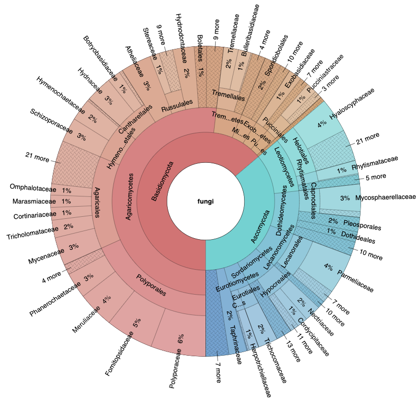
Figure 4: Fungal taxonomic composition and marginal species occurrence probabilities.

The matrix $\bm{\Sigma}$ captures dependence in co-occurrence, which is of interest in studying species interactions. Considering the correlation coefficients different from zero based on $90\%$ credible intervals, the correlation matrix exhibits a sparse structure. While it is difficult to interpret the results on the species level due to the large dimensionality, we can obtain interesting conclusions by grouping species that fall in the same branch of the taxonomic tree; for example, species of the same order. As illustration, we focus on order pairs exhibiting the highest relative frequency of correlations different from zero. Relative frequency refers to the total positive (or negative) correlations between two orders among all possible pairs of these two orders. We notice that different orders of lichenized fungi (Lücking et al., 2017) exhibit a positive correlation. In terms of positive relative frequency, the $33\%$ of (Lecideales, Pertusariales) and (Umbilicariales, Phaeomoniellales), the $25\%$ of (Lecideales, Baeomycetales), and the $23\%$ of (Xylariales, Lecideales) are correlated in occurrence. Perhaps, environmental conditions that support one type of lichen are also favorable for other types. Another important group is mycorrhizal fungi, which are in symbiotic relationships with plant roots. We notice a positive correlation ($50\%$ in terms of positive relative frequency) between the Sebacinales and Cantharellales orders of mycorrhizal fungi, likely due to the fact that both orders tend to form relationships with similar plant species such as orchids (Qin et al., 2020) which are widespread in Finland.

In biodiversity research, it is important to measure species richness, corresponding to the number of species in a community (Colwell, 2009). A commonly employed methodology for this purpose involves constructing species accumulation curves. These curves record the cumulative number of species found in an area as a function of the cumulative sampling effort. Initially, the curves exhibit a steep ascent as more samples are collected, but after the initial stages the curves are expected to exhibit a slower growth pattern, indicative of the inclusion of increasingly rare species. For a Bayesian nonparametric method that directly specifies a model for the accumulation curve see Zito et al. (2023).

With this motivation, we estimate the sample species richness $p_{n}^{*}$ under our model for Site 1 and Site 2, as the other sites have few samples. For Site 1, we randomly select a test set containing $25\%$ of the observations and fit the MVP-IBP model excluding these observations. Then, we draw 100 samples from the predictive distributions of $\bm{Y}$ and count the cumulative total number of species across the different sample sizes, estimating $p^{*}_{n}$ for each $n=1,\dots,n_{1}$ with $n_{1}$ the total number of observations in the test set for Site 1. We compare to results from IBP and hierarchical bigMVP (Chakraborty et al., 2023). For the IBP, we consider the same test set, but only use observations from Site 1 in training. To evaluate the models, we compute for each $n$ $(n=1,\dots,n_{1})$ a predictive mean square error for $p^{*}_{n}$. We followed the same procedure for Site 2. Table 1 shows, for the two sites, the median and the interquartile range of the above mean square errors computed from the different points in the test sets. The MVP-IBP model consistently outperforms the competitors in predicting $p^{*}_{n}$ for both sites.

Table 1: Performance of the MVP-IBP, bigMVP and IBP models in predicting discovery of new species of fungi in Finland for Site 1 and Site 2 in terms of MSE using logarithm scale.

	Site 1			Site 2
	MVP-IBP	IBP	bigMVP	MVP-IBP	IBP	bigMVP
MSE $p^{*}_{n}$ (median)	4.75	8.78	7.86	5.81	8.19	7.50
MSE $p^{*}_{n}$ (IQR)	0.09	0.04	0.14	0.99	0.72	0.61

6 Discussion

In this article we propose a novel class of MVP-IBP models for inference on multivariate binary outcomes having a growing dimension. While the developments were concretely motivated by biodiversity studies, the modeling framework has much broader applicability. The MVP-IBP class maintains many of the desirable properties of the popular IBP, while addressing important statistical complexities that arise in applications, such as dependence in feature (species) occurrence, covariate effects and the need to borrow information in conducting inferences for rare features (species).

In introducing a class of IBP-type models that allow a flexible dependence structure across features, we are faced with a challenge of how to effectively characterize an increasing-dimensional correlation matrix. In fixed dimensional settings, it is common to rely on latent factor models to reduce dimensionality in characterizing dependence in multivariate binary data. However, such approaches cannot be directly applied in the IBP setting, which inevitably involves extremely sparse binary data and requires a coherent framework for prediction. We propose two main alternative approaches for addressing this problem, including novel modifications to factor models and direct hierarchical modeling of the elements of the correlation matrix. These initial directions should motivate more work in this area; for example, alternative factor modeling approaches (perhaps related to Beraha and Griffin (2023)) or stochastic block model formulations that infer latent communities of species based on their correlation structure.

There are many interesting directions for future research motivated directly by biodiversity studies. Firstly, most current IBP models impose a restrictive rate of discovery of new features as additional samples are taken. However, in exploratory data analyses, we found that fitting the empirical species accumulation curves from real world biodiversity studies often requires more flexibility. One promising direction in this regard is to introduce dependence in more sophisticated versions of the IBP, such as the three-parameter generalization with power-law behaviour of Teh and Gorur (2009).

Another important direction is making our statistical tools sufficiently computationally efficient and off-the-shelf so that ecologists can use them routinely. Joint species distribution models (JSDMs) have become routinely used in ecology, but their inference methods cannot handle new species discovery and/or the presence of many rare species in the sample. It is of substantial importance to be able to predict future species discovery based on current samples, while accurately characterizing uncertainty and accommodating effects of climate change and other covariates. It is additionally of substantial interest to infer which species are endangered and should be add to so-called red lists. Our statistical tools provide a first step towards automating such inferences and decisions.

Supplementary materials

S.1 Proofs

S.1.1 Proof of Theorem 1

We start by computing the $p$ limit of the expected value of $n_{i}=\sum_{j=1}^{p}y_{ij}$. Let $\phi(\cdot)$ denote the density function of a standard normal variable. The expected value of the number of features per object $n_{i}$ is

$$E(n_{i})=\sum_{j=1}^{p}\int_{-\infty}^{\infty}\Phi(\beta_{j})\frac{1}{\tau_{p}}\phi\left(\frac{\beta_{j}-\mu_{p}}{\tau_{p}}\right)\,d\beta_{j}=\sum_{j=1}^{p}\int_{-\infty}^{\infty}\Phi(\tau_{p}\beta_{j}+\mu_{p})\phi(\beta_{j})\,d\beta_{j}.$$ (12)

Owen (1980) showed that (12) is equal to $\sum_{j=1}^{p}\Phi(\mu_{p}/[1+\tau_{p}^{2}]^{1/2})$. Then, by substituting $\mu_{p}$ in the latter expression we obtain

$$E(n_{i})=p\frac{\alpha/p}{\alpha/p+1},$$

that converges to $\alpha$ as $p\to\infty$ for each $i=1,\dots,n$.

If we further assume $\bm{\Sigma}=\bm{I}$, then $n_{i}$ is a sum of independent Bernoulli random variables and thus it is a binomial distribution with size $p$ and success probability $\frac{\alpha/p}{\alpha/p+1}$. Given that $p\frac{\alpha/p}{\alpha/p+1}$ converges to $\alpha$ for $p\to\infty$, it follows by the law of rare events that $n_{i}$ converges to a Poisson distribution of parameter $\alpha$.

S.1.2 Proof of Proposition 1

Recalling that the observations for different features are not independent, the variance of $n_{i}=\sum_{j=1}^{p}y_{ij}$ is $\mathrm{var}(n_{i})=\sum_{j=1}^{p}\mathrm{var}(y_{ij})+\sum_{j<j^{\prime}\leq p}\mathrm{cov}(y_{ij},y_{ij^{\prime}})$, where

$$\mathrm{cov}(y_{ij},y_{ij^{\prime}})=E(y_{ij}y_{ij^{\prime}})-\frac{p(p-1)}{2}\frac{\alpha^{2}}{(\alpha+p)^{2}},$$

and applying the law of total variance, the variance of the observations is

$$\mathrm{var}(y_{ij})=E(\Phi(\beta_{j})[1-\Phi(\beta_{j})])+\mathrm{var}(\Phi(\beta_{j}))=E(\Phi(\beta_{j}))-E(\Phi(\beta_{j}))^{2}=\frac{\alpha}{\alpha+p}-\frac{\alpha^{2}}{(\alpha+p)^{2}}.$$

From the last equation it easily follows that $\lim_{p\to\infty}\sum_{j=1}^{p}\mathrm{var}(y_{ij})=\alpha$. Note that this is the variance of $n_{i}$ if one assumes independence among features, i.e. the covariance between $y_{ij}$ and $y_{ij^{\prime}}$ is zero. Thus, the limit for $p\to\infty$ of the variance of $n_{i}$ is

$$\lim_{p\to\infty}\mathrm{var}(n_{i})=\alpha-\frac{\alpha^{2}}{2}+\lim_{p\to\infty}\sum_{j<j^{\prime}\leq p}E(y_{ij}y_{ik}).$$ (13)

In the following we will focus on the more challenging part of obtaining an analytical expression for the $p$ limit of $E(y_{ij}y_{ik})$, which involves a bivariate Gaussian orthant probability. The expected value of the product of $y_{ij}$ and $y_{ij^{\prime}}$ is

$$E(y_{ij}y_{ij^{\prime}})=E(\Phi_{2}(\beta;\sigma_{jj^{\prime}}))=\int_{-\infty}^{\infty}\int_{-\infty}^{\infty}\Phi_{2}(\beta;\sigma_{jj^{\prime}})\frac{1}{\tau_{p}}\phi\left(\frac{\beta_{j}-\mu_{p}}{\tau_{p}}\right)\frac{1}{\tau_{p}}\phi\left(\frac{\beta_{j}^{\prime}-\mu_{p}}{\tau_{p}}\right)\,d\beta_{j}\,d\beta_{j}^{\prime},$$ (14)

where $\Phi_{2}(\beta;\sigma_{jk})$ is the cumulative distribution function of a bivariate normal evaluated in $\beta=(\beta_{j},\beta_{j^{\prime}})^{\top}$ with mean zero and correlation $\sigma_{jk}$. Drezner and Wesolowsky (1990) showed that the cumulative distribution function of a bivariate normal can be written as

$$\Phi_{2}(\beta;\sigma_{jj^{\prime}})=\Phi(\beta_{j})\Phi(\beta_{j}^{\prime})+\frac{1}{2\pi}I(\sigma_{jj^{\prime}}),$$

where

$$I(\sigma_{jj^{\prime}})=\int_{0}^{\sigma_{jj^{\prime}}}\frac{1}{\sqrt{1-z^{2}}}\exp\left\{-\frac{1}{2(1-z^{2})}(\beta_{j}^{2}-2\beta_{j}\beta_{j^{\prime}}z+\beta_{j^{\prime}}^{2})\right\}dz.$$

Then leveraging the same result on integrals of normal cumulative distribution function (Owen, 1980) used in the proof of Theorem 1, equation (14) becomes

$$E(y_{ij}y_{ij^{\prime}})=\frac{\alpha^{2}}{(\alpha+p)^{2}}+\frac{1}{2\pi}\int_{-\infty}^{\infty}\int_{-\infty}^{\infty}I(\sigma_{jj^{\prime}})\frac{1}{\tau_{p}}\phi\left(\frac{\beta_{j}-\mu_{p}}{\tau_{p}}\right)\frac{1}{\tau_{p}}\phi\left(\frac{\beta_{j^{\prime}}-\mu_{p}}{\tau_{p}}\right)\,d\beta_{j}\,d\beta_{j^{\prime}}.$$

The latter result implies that, as $p$ grows, the variance of $n_{i}$ in (13) becomes

$$\lim_{p\to\infty}\mathrm{var}(n_{i})=\alpha+\lim_{p\to\infty}\sum_{j<j^{\prime}\leq p}\frac{1}{2\pi}\int_{-\infty}^{\infty}\int_{-\infty}^{\infty}I(\sigma_{jj^{\prime}})\frac{1}{\tau_{p}}\phi\left(\frac{\beta_{j}-\mu_{p}}{\tau_{p}}\right)\frac{1}{\tau_{p}}\phi\left(\frac{\beta_{j^{\prime}}-\mu_{p}}{\tau_{p}}\right)\,d\beta_{j}\,d\beta_{j^{\prime}}.$$ (15)

By dominated convergence theorem, we first compute the limit of the integrand in $\eqref{eq:limp_vni}$ and then do the integration. Let $a_{p}\simeq b_{p}$ indicate that $\lim_{p\to\infty}a_{p}/b_{p}=1$, that is $a_{p}$ and $b_{p}$ have the same order. Exploiting the following asymptotic expansion (Abramowitz and Stegun, 1948) for the inverse of the cumulative distribution function of a normal distribution

$$\Phi^{-1}(x)\simeq-\sqrt{-2\log x-\log(-2\log x)-\log(2\pi)}+o(1),\quad x\rightarrow 0,$$

we have $\mu_{p}\simeq-[(1+\tau_{p}^{2})(-2\log(\alpha/(\alpha+p))-\log(-2\log(\alpha/(\alpha+p)))-\log(2\pi))]^{-1/2}$ for $p\rightarrow\infty$. Then, by standard convergence theorems we obtain the following equivalence

$$\lim_{p\to\infty}\frac{1}{\tau_{p}}\phi\left(\frac{\beta_{j}-\mu_{p}}{\tau_{p}}\right)\frac{1}{\tau_{p}}\phi\left(\frac{\beta_{j}^{\prime}-\mu_{p}}{\tau_{p}}\right)=\lim_{p\to\infty}\exp\{-(1+\beta_{j}+\beta_{j}^{\prime})\}\frac{\alpha^{2}}{(\alpha+p)^{2}},$$

from which follows that the limit in (15) is equal to

$$\lim_{p\to\infty}\mathrm{var}(n_{i})=\alpha+\lim_{p\to\infty}\exp\{-1\}\frac{\alpha^{2}}{(\alpha+p)^{2}}\sum_{j<j^{\prime}\leq p}\frac{1}{2\pi}\int_{-\infty}^{\infty}\int_{-\infty}^{\infty}I(\sigma_{jj^{\prime}})\exp\{-\beta_{j}\}\exp\{-\beta_{j}^{\prime}\}\,d\beta_{j}d\beta_{j^{\prime}}.$$

Interchanging the order of integration with Fubini-Tonelli theorem, the integrals in the latter expression become

$$\int_{0}^{\rho_{jj^{\prime}}}\int_{-\infty}^{\infty}\int_{-\infty}^{\infty}\frac{1}{\sqrt{1-z^{2}}}\exp\left\{-\frac{1}{2(1-z^{2})}(\beta_{j}^{2}-2\beta_{j}\beta_{j^{\prime}}z+\beta_{j^{\prime}}^{2})\right\}\exp\{-\beta_{j}\}\exp\{-\beta_{j}^{\prime}\}\,d\beta_{j}\,d\beta_{j^{\prime}}dz.$$ (16)

By completing the square for both $\beta_{j}$ and $\beta_{j}^{\prime}$, we derive expressions that resemble the kernels of two normal densities and the subsequent integration with respect to both $\beta_{j}$ and $\beta_{j}^{\prime}$ becomes straightforward. Then, by algebraic simplifications (16) can be expressed as $2\pi e\int_{0}^{\sigma_{jj^{\prime}}}\exp\{z\}dz=2\pi e|\exp\{\sigma_{jj^{\prime}}\}-1|$. We included the absolute value in the latter expression to consider both positive and negative correlations. Thus, as $p$ grows the variance of $n_{i}$ can be written as

$$\lim_{p\to\infty}\mathrm{var}(n_{i})=\alpha+\lim_{p\to\infty}\frac{\alpha^{2}}{(\alpha+p)^{2}}\sum_{j<j^{\prime}\leq p}|\exp\{\sigma_{jj^{\prime}}\}-1|.$$

If we assume a finite number of correlation coefficient, i.e. $\sigma_{jj^{\prime}}\in\{\rho_{1},\ldots,\rho_{K}\}$ with $K\in\mathds{N}$, then $\sum_{j<j^{\prime}\leq p}|\exp\{\sigma_{jj^{\prime}}\}-1|=\sum_{k=1}^{K}w_{k}|\exp\{\rho_{k}\}-1|$, with $w_{k}=\sum_{j<j^{\prime}\leq p}\mathds{1}(\sigma_{jj^{\prime}}=\rho_{k})$ and $\sum_{k=1}^{K}w_{k}=p(p-1)/2$. Finally, considering that $\sum_{k=1}^{K}w_{k}|\exp\{\rho_{k}\}-1|$ is bounded above by $(\underset{k}{\mathrm{max}}\,|\exp\{\rho_{k}\}-1|)p(p-1)/2$ and below by $(\underset{k}{\mathrm{min}}\,|\exp\{\rho_{k}\}-1|)p(p-1)/2$, we can conclude that

$$\alpha+\alpha^{2}/2\,(\underset{k}{\mathrm{min}}\,|\exp\{\rho_{k}\}-1|)\leq\lim_{p\to\infty}\mathrm{var}(n_{i})\leq\alpha+\alpha^{2}/2\,(\underset{k}{\mathrm{max}}\,|\exp\{\rho_{k}\}-1|).$$

S.1.3 Proof of Proposition 3

The target is computing the $p\to\infty$ limit of the expected value of the number of common species

$$E(c^{(\epsilon)})=\sum_{j=1}^{p}\mathrm{pr}(\Phi(\beta_{j})>\epsilon)=\sum_{j=1}^{p}\mathrm{pr}(\beta_{j}>\Phi^{-1}(\epsilon))=p\left[1-\Phi\left(\frac{\Phi^{-1}(\epsilon)-\mu_{p}}{\tau_{p}}\right)\right].$$ (17)

Exploiting the following asymptotic expansion (Abramowitz and Stegun, 1948) for the cumulative distribution function of a normal distribution

$$1-\Phi(x)\simeq\frac{\exp\{-x^{2}/2\}}{\sqrt{2\pi}x}\left(1-\frac{1}{x^{2}}+o\left(\frac{1}{x^{4}}\right)\right),\quad x\rightarrow\infty,$$

the limit of the expected value of $c^{(\epsilon)}$ can be equivalently written as

$$\lim_{p\rightarrow\infty}E(c^{(\epsilon)})=\lim_{p\rightarrow\infty}\frac{p\tau_{p}}{\sqrt{2\pi}(\epsilon^{*}-\mu_{p})}\exp\left\{-\frac{1}{2\tau_{p}^{2}}(\epsilon^{*}-\mu_{p})^{2}\right\},$$ (18)

with $\epsilon^{*}=\Phi^{-1}(\epsilon)$. Then, by leveraging the same asymptotic expansion for the inverse of the cumulative distribution function of a normal distribution used in the proof of Proposition 1, with standard convergence theorems we obtain

$$\exp\left\{-\frac{1}{2\tau_{p}^{2}}(\epsilon^{*}-\mu_{p})^{2}\right\}\simeq\lim_{p\to\infty}\exp\{-\epsilon^{*}\}\left(\frac{\alpha}{\alpha+p}\right)\sqrt{-2\log\left(\frac{\alpha}{\alpha+p}\right)}\sqrt{2\pi}\,\exp\{-1/2\},$$

and

$$\frac{\tau_{p}}{\epsilon^{*}-\mu_{p}}\simeq\frac{1}{\sqrt{-2\log(\alpha/(\alpha+p))}}.$$

Thus, we can conclude that the limit of the expected number of common species as $p$ grows is

$$\lim_{p\rightarrow\infty}\exp\left\{-\epsilon^{*}-\frac{1}{2}\right\}p\left(\frac{\alpha}{\alpha+p}\right)\sqrt{-2\log\left(\frac{\alpha}{\alpha+p}\right)}\frac{1}{\sqrt{-2\log(\alpha/(\alpha+p))}}=\alpha\exp\left\{-\epsilon^{*}-\frac{1}{2}\right\}.$$

S.1.4 Proof of Theorem 2

Let $w_{j}=\mathds{1}(n_{j}>0)$, with $n_{j}=\sum_{i=1}^{n}y_{ij}$, be binary random variables that indicate if column $j$ is non empty, for $j=1,\dots,p$. Then the number of non-empty columns is $p^{*}=\sum_{j=1}^{p}w_{j}$, where $w_{j}\sim Be(1-(1-\pi_{j})^{n})$ with $\pi_{j}=\Phi(\beta_{j})$ the marginal success probabilities. Therefore, the aim is to compute the following limit

$$L(p^{*})=\lim_{p\to\infty}E(p^{*})=\lim_{p\to\infty}\sum_{j=1}^{p}E(w_{j})=\lim_{p\to\infty}\sum_{j=1}^{p}E(1-(1-\pi_{j})^{n}).$$ (19)

Exploiting the binomial sum properties we can write $(1-\pi_{j})^{n}=\sum_{k=0}^{n}\binom{n}{k}(-1)^{k}\pi_{j}^{k}\,$. Hence, $L(p^{*})$ in (19) can be equivalently written as $\lim_{p\to\infty}\sum_{j=1}^{p}(-\sum_{k=1}^{n}\binom{n}{k}(-1)^{k}E(\pi_{j}^{k}))$. Leveraging on the Owen’s integral table results (Owen, 1980), we can obtain a closed form for the expected value of the marginal probabilities $\pi_{j}$ raised to $k$

$$E(\pi_{j}^{k})=\int_{-\infty}^{\infty}\Phi(\beta_{j})^{k}\frac{1}{\tau_{p}}\phi\left(\frac{\beta_{j}-\mu_{p}}{\tau_{p}}\right)\,d\beta_{j}=\Phi_{k}(\mu_{p}\bm{1}_{k};\bm{V}_{p}),$$

where $\bm{V}_{p}=\bm{I}_{k}+\tau_{p}^{2}\bm{1}_{k}^{\top}\bm{1}_{k}$ is a $k\times k$ covariance matrix, $\bm{1}_{k}$ denotes a $k-$dimensional vector of all ones and $\Phi_{k}(\mu_{p}\bm{1}_{k};\bm{V}_{p})$ denote the cumulative distribution function of the multivariate Gaussian $N_{k}(\bf{0}_{k},\bm{V}_{p})$ evaluated at $\mu\bm{1}_{k}$. Hence, the target quantity to compute $L(p^{*})$ becomes

$$L(p^{*})=\lim_{p\to\infty}p\left(-\sum_{k=1}^{n}\binom{n}{k}(-1)^{k}\Phi_{k}(\mu_{p}\bm{1}_{k};\bm{V}_{p})\right).$$ (20)

We will focus on the most challenging part of computing $\lim_{p\to\infty}\Phi_{k}(\mu_{p}\bm{1}_{k};\bm{V}_{p})$. Let $\bm{x}=(x_{1},\dots,x_{k})^{\top}$ and recall that $\bm{V}_{p}^{-1}$ has diagonal elements equal to $(\tau_{p}^{2}[k-1]+1)/(k\tau_{p}^{2}+1)$ and off-diagonal elements equal to $-\tau_{p}^{2}/(k\tau^{2}_{p}+1)$. Then we have

$$\Phi_{k}(\mu_{p}\bm{1}_{k};\bm{V}_{p}) =\frac{|\bm{V}_{p}|^{-1/2}}{(2\pi)^{k/2}}\int_{-\infty}^{0}\dots\int_{-\infty}^{0}\exp\left\{-\frac{1}{2}(\bm{x}+\mu_{p}\bm{1}_{k})^{\top}\bm{V}_{p}^{-1}(\bm{x}+\mu_{p}\bm{1}_{k})\right\}dx$$

$$=\frac{(1+k\tau_{p}^{2})^{-1/2}}{(2\pi)^{k/2}}\exp\left\{-\frac{1}{2}\mu_{p}^{2}\bm{1}_{k}^{\top}\bm{V}_{p}^{-1}\bm{1}_{k}\right\}\int_{-\infty}^{0}\dots\int_{-\infty}^{0}\exp\left\{-\frac{1}{2}\bm{x}\bm{V}_{p}^{-1}\bm{x}^{\top}-\bm{x}\bm{V}_{p}^{-1}\mu_{p}\bm{1}_{k}\right\}dx$$

$$=\frac{(1+k\tau_{p}^{2})^{-1/2}}{(2\pi)^{k/2}}\exp\left\{-\frac{1}{2}\,\frac{k\mu_{p}^{2}}{k\tau_{p}^{2}+1}\right\}\int_{-\infty}^{0}\dots\int_{-\infty}^{0}\exp\left\{-\frac{1}{2}\bm{x}\bm{V}_{p}^{-1}\bm{x}^{\top}-\frac{\mu_{p}}{k\tau_{p}^{2}+1}\bm{x}\bm{1}_{k}\right\}dx.$$

Notice that as $p\to\infty$, the integral above, by standard convergence theorems, converges to

$$\int_{-\infty}^{0}\dots\int_{-\infty}^{0}\exp\left\{-\frac{1}{2}\sum_{i=1}^{k}x_{i}\left(\frac{k-1}{k}x_{i}+\frac{1}{k}\sum_{j\neq i}x_{j}\right)-\frac{1}{k}\bm{x}^{\top}\bm{1}_{k}\right\}dx=C_{k},$$

where $C_{k}$ is a generic constant depending on $k$. Then by using the same asymptotic expansion for $\Phi^{-1}(\alpha/[\alpha+p])$ stated in the proof of Proposition 1, for $p\to\infty$ it holds

$$\frac{(1+k\tau_{p}^{2})^{-1/2}}{(2\pi)^{k/2}}\exp\left\{-\frac{1}{2}\,\frac{k\mu_{p}^{2}}{k\tau_{p}^{2}+1}\right\} \simeq\frac{(1+k2\log p)^{-1/2}}{(2\pi)^{k/2}}\left(\frac{\alpha}{\alpha+p}\right)\sqrt{-2\log\left(\frac{\alpha}{\alpha+p}\right)}\exp\{-1/2\}\sqrt{2\pi}.$$

From the latter equation it easily follows that $\Phi_{k}(\mu_{p}\bm{1}_{k};\bm{V}_{p})\simeq(\alpha/(\alpha+p))C_{k}$ for $p\to\infty$. Then substituting $\Phi_{k}(\mu_{p}\bm{1}_{k};\bm{V}_{p})$ in (20) we obtain

$$L(p^{*})=\lim_{p\to\infty}p\left(-\sum_{k=1}^{n}\binom{n}{k}(-1)^{k}\left(\frac{\alpha}{\alpha+p}\right)C_{k}\right)=\alpha\left(-\sum_{k=1}^{n}\binom{n}{k}(-1)^{k}C_{k}\right),$$ (21)

which shows that the $p$ limit of the expected value of $p^{*}$ converges to a finite value.

Obtaining an expression for $C_{k}$ involves integrating a multivariate normal probability and explicit formulas of orthant probability are only available for small values of $k$. However, leveraging the method proposed in Genz (1992) we can obtain a numerical evaluation of $C_{k}$. Recalling that the harmonic number can be written as $H_{n}=-\sum_{k=1}^{n}\binom{n}{k}(-1)^{k}\frac{1}{k}$, we have

$$L(p^{*})=\alpha\left(H_{n}\ +\sum_{k=1}^{n}\binom{n}{k}(-1)^{k}d(k)\right),$$

where $d(k)=C_{k}-1/k$. The function $d(k)$ for $k\in(1,1000)$ is a unimodal function; see Figure S1 for a graphical representation. We considered the function for $k\in(1,1000)$ as this is a reasonable set of values for the sample size. Note also that for $k=1$ the orthant probability has an analytical solution and $d(k)=0$. Given that $\sum_{k=1}^{n}\binom{n}{k}(-1)^{k}=-1$, we can obtain the following bounds for the limit of the expected value of $p^{*}$

$$\alpha(H_{n}-m_{k})<L(p^{*})<\alpha(H_{n}-u_{k}),\quad\text{where}\quad u_{k}=\underset{k\in(1,1000)}{\mathrm{max}}\,d(k),\,m_{k}=\underset{k\in(1,1000)}{\mathrm{min}}\,d(k),$$

with $u_{k}=0.02$ and $m_{k}=0.073$. Therefore, considering that $H_{n}=\mathcal{O}(\log n)$, we can conclude that $L(p^{*})=\mathcal{O}(\alpha\log n)$.

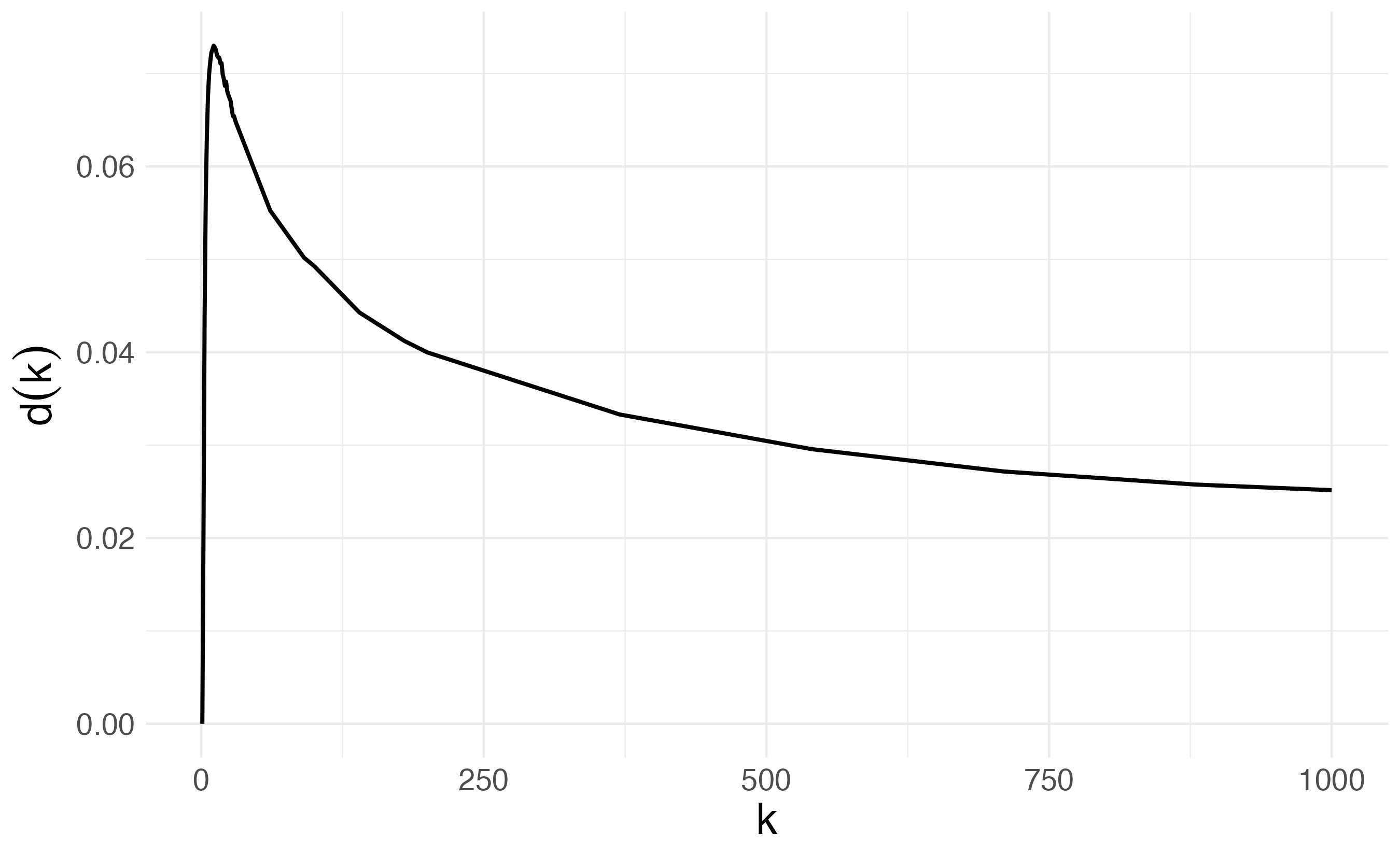
Figure S1: Graphical representation of the function $d(k)$.

In the following part we will prove that, assuming independence among features, the number of non empty columns converges to a Poisson distribution as $p$ grows. Assuming $\bm{\Sigma}=\bm{I}$ implies that $p^{*}$ is a sum of independent Bernoulli random variables $\omega_{j}$, and thus it is a binomial distribution with size $p$ and success probability $c_{p}=-\sum_{k=1}^{n}\binom{n}{k}(-1)^{k}\left(\frac{\alpha}{\alpha+p}\right)C_{k}$. Given that $pc_{p}$ converges to $l=\alpha(-\sum_{k=1}^{n}\binom{n}{k}(-1)^{k}C_{k})$ for $p\to\infty$, it follows by the law of rare events that $p^{*}$ converges to a Poisson distribution of parameter $l$.

S.1.5 Proof of Theorem 3

The expected value of the number of features per object $n_{i}=\sum_{j=1}^{p}y_{ij}$ for the covariate-dependent MVP-IBP is

$$E(n_{i})=\sum_{j=1}^{p}E(y_{ij})=\sum_{j=1}^{p}\int_{-\infty}^{\infty}\Phi(V_{ij})\frac{1}{\sqrt{\tau_{p}^{2}+\bm{x}_{i}^{\top}\bm{\Psi}\bm{x}_{i}}}\phi\left(\frac{V_{ij}-\bm{x}_{i}^{\top}\bm{\gamma}-\mu_{p}}{\sqrt{\tau_{p}^{2}+\bm{x}_{i}^{\top}\bm{\Psi}\bm{x}_{i}}}\right)\,dV_{ij},$$ (22)

and following the proof of Theorem 1 we can show that (22) is equal to

$$\sum_{j=1}^{p}\Phi\left(\frac{\mu_{p}+\bm{x}_{i}^{\top}\bm{\gamma}}{\sqrt{1+\tau_{p}^{2}+\bm{x}_{i}^{\top}\bm{\Psi}\bm{x}_{i}}}\right).$$ (23)

The $p\to\infty$ limit of the latter equation can be computed by employing the same asymptotic expansions for $\mu_{p}$ and $\Phi(\cdot)$ used in the proof of propositions 1 and 3 and it is equal to

$$\lim_{p\to\infty}p\,\Phi\left(\frac{\mu_{p}+\bm{x}_{i}^{\top}\bm{\gamma}}{\sqrt{1+\tau_{p}^{2}+\bm{x}_{i}^{\top}\bm{\Psi}\bm{x}_{i}}}\right) =\lim_{p\to\infty}\alpha\exp\{\bm{x}_{i}^{\top}\bm{\gamma}-1/2\}p\left(\frac{\alpha}{\alpha+p}\right)^{\frac{1+2\log p+\bm{x}_{i}^{\top}\bm{\Psi}\bm{x}_{i}}{1+2\log p+}}$$

$$=\alpha\exp\{\bm{x}_{i}^{\top}\bm{\gamma}+\frac{1}{2}(\bm{x}_{i}^{\top}\bm{\Psi}\bm{x}_{i}-1)\}.$$

Given this observation, the second point of Theorem 3 can be easily shown by simply adapting the proof of Proposition 1.

S.1.6 Proof of Proposition 4

The expected value of the number of common species for sample $i$ for the covariate-dependent setting is

$$E(c_{i}^{\epsilon})=\sum_{j=1}^{p}\mathrm{pr}(\Phi(\beta_{j}+\bm{x}_{i}^{\top}\bm{b}_{j})>\epsilon)=\sum_{j=1}^{p}\mathrm{pr}(\beta_{j}+\bm{x}_{i}^{\top}\bm{b}_{j}>\Phi^{-1}(\epsilon)),$$ (24)

and thus the focus is computing the following limit

$$\lim_{p\to\infty}p\left[1-\Phi\left(\frac{\Phi^{-1}(\epsilon)-\mu_{p}-\bm{x}_{i}^{\top}\bm{\gamma}}{\sqrt{\tau_{p}+\bm{x}_{i}^{\top}\bm{\Psi}\bm{x}_{i}}}\right)\right].$$

Rewriting the above expression as

$$\lim_{p\to\infty}p\left[\Phi\left(\frac{\mu_{p}+(\bm{x}_{i}^{\top}\bm{\gamma}-\Phi^{-1}(\epsilon))}{\sqrt{\tau_{p}+\bm{x}_{i}^{\top}\bm{\Psi}\bm{x}_{i}}}\right)\right],$$

we obtain a similar expression to equation (23) in the proof of Proposition 3. Hence, substituting in (23) $\bm{x}_{i}^{\top}\bm{\gamma}+\Phi^{-1}(\epsilon)$ in place of $\bm{x}_{i}^{\top}\bm{\gamma}$, the procedure to compute the limit is the same. Therefore we conclude that

$$\lim_{p\to\infty}E(c_{i}^{\epsilon})=\alpha\exp\{-\Phi^{-1}(\epsilon)+\bm{x}_{i}^{\top}\bm{\gamma}+\frac{1}{2}(\bm{x}_{i}^{\top}\bm{\Psi}\bm{x}_{i}-1)\}.$$

S.2 Posterior computations

Algorithm 1 summarizes the steps to obtain empirical Bayes estimation of $\alpha$ and $\omega$ to sample from the hierarchical MVP-IBP model described in Section 3.1 of the main document. In the common correlation coefficient case, the algorithm can be simplified as we do not need to estimate $\omega$; hence, we only repeat steps 1-3.

Initialize $\omega$ and $\alpha$.

1. Given $\alpha$ obtain approximation to $\Pi(\beta_{j}\mid y,\alpha)$ as $N(\hat{\beta}_{j},\bm{Q}_{j})$ for $j=1,\dots,P$ with the prior $\beta_{j}\sim N(\mu_{P},\tau_{P})$.

2. Draw $\beta_{j}\sim N(\hat{\beta}_{j},\bm{Q}_{j})$ independently for $j=1,\dots,P$.

3. Update $\alpha$ through a Metropolis–Hastings step.

4. Given $\omega$, obtain approximations to $\Pi(\sigma_{jj^{\prime}}\mid y,\omega)$ as $N(\hat{\sigma}_{jj^{\prime}},s_{jk}^{2})$ for $j<j^{\prime}=1,\dots,P$ with pseudo-priors $\Pi_{j}^{*}(\beta_{j}\mid y)\Pi_{j^{\prime}}^{*}(\beta_{j^{\prime}}\mid y)$.

5. Draw $\sigma_{jj^{\prime}}\sim N(\hat{\sigma}_{jj^{\prime}},s_{jk}^{2})$ independently and set $\zeta_{jj^{\prime}}=0.5\log[(1+\sigma_{jj^{\prime}})/(1-\sigma_{jj^{\prime}})]$ for $j<j^{\prime}=1,\dots,P$.

6. Update $\omega^{2}\sim IG\left(\frac{P(P-1)}{2}+a_{\omega},\frac{1}{2}\sum_{j<j^{\prime}}\zeta_{jj^{\prime}}^{2}+b_{\omega}\right)$

Repeat steps 1-6 T times to obtain T samples of $\omega$ and $\alpha$.

Algorithm 1 Two-stage approximate conditional sampler for the hierarchical MVP-IBP.

Algorithm 2 summarizes the steps for the Gibbs sampler to compute the MVP-IBP factor model truncated at $P$ species described in Section 3.2 of the main document. The Gibbs sampler is combined with a Metropolis-Hastings step for updating the parameter $\alpha$. For sampling from the CUSP prior Legramanti et al. (2020) rely on a data augmentation scheme, introducing independent indicators $S_{k}$ ($k=1,\dots,K$) having $\mathrm{pr}(S_{k}=l\mid\omega_{l})=\omega_{l}$ ($l=1,\dots,K$). Given these indicators, it is possible to sample the other parameters from conjugate full conditional distributions, while the updating of $S_{1},\dots,S_{K}$ relies on

$$\mathrm{pr}(S_{k}=l\mid-)\propto\begin{cases}\omega_{l}N_{P}(\bm{\lambda}_{k};0,\theta_{\infty}\bm{I}_{P})&l=1,\dots,k\\ \omega_{l}t_{2a_{\theta}}(\bm{\lambda}_{k};0,(b_{\theta}/a_{\theta})\bm{I}_{P})&l=k+1,\dots,K,\end{cases}$$ (25)

where $t_{2a_{\theta}}(\bm{\lambda}_{k};0,(b_{\theta}/a_{\theta})\bm{I}_{P})$ is the density of a P-variate Student-t distribution evaluated at $\bm{\lambda}_{k}=(\lambda_{1k},\dots,\lambda_{Pk})^{\top}$. To invert the correlation matrix $\bm{\Sigma}$ in the updating of $\tilde{\bm{\beta}}$, we use the Sherman–Morrison–Woodbury formula (Hager, 1989), that speeds up the computation.

1. For $i=1$ to $i=n$ and for $j=1$ to $j=P$ sample the entries of $\bm{Z}$ from

   $$z_{ij}\mid-\sim\begin{cases}TN_{[0,\infty)}(\beta_{j}+\bm{\lambda}_{j}^{\top}\bm{\eta}_{i},1)&\text{if $y_{ij}=1$},\\ TN_{(-\infty,0)}(\beta_{j}+\bm{\lambda}_{j}^{\top}\bm{\eta}_{i},1)&\text{if $y_{ij}=0$},\end{cases}$$

   where $TN_{[0,\infty)}(\cdot)$ is a normal density truncated to the region $[0,\infty)$.

2. For $i=1$ to $i=n$ sample $\bm{\eta}_{i}$ from $N_{k}(\bm{V}_{\eta}\bm{\Lambda}^{\top}(\bm{z}_{i}-\bm{\beta}),\bm{V}_{\eta}),\text{ with }\bm{V}_{\eta}=(\bm{\Lambda}^{\top}\bm{\Lambda}+\bm{I}_{k})^{-1}$.

3. For $j=1$ to $j=P$ sample the $j$th row of $\bm{\Lambda}$ from $N_{K}(\bm{V}_{\lambda}\bm{\eta}^{\top}(\bm{z}_{j}-\bm{\beta}_{j}\bm{1}_{n}),\bm{V}_{\lambda})$, with $\bm{V}_{\lambda}=(\bm{D}^{-1}+\bm{\eta}^{\top}\bm{\eta})^{-1}$ and $\bm{D}=\mathrm{diag}(\theta_{1},\dots,\theta_{K})$.

4. Sample $\tilde{\bm{\beta}}$ from $N_{P}(\bm{V}_{\beta}(\tau^{-2}_{P}\bm{I}_{P}\mu_{P}+n\bm{\Sigma}^{-1}\bar{\bm{z}}),\bm{V}_{\beta})$, with $\bm{V}_{\beta}=(\tau^{-2}_{P}\bm{I}_{P}+n\bm{\Sigma}^{-1})^{-1}$ and $\bar{\bm{z}}=\frac{1}{n}\sum_{i=1}^{n}\bm{z}_{i}$ where $\bm{z}_{i}^{\top}=(z_{i1},\dots,z_{iP})$.

5. Update $\alpha$ using a Metropolis-Hastings step within the Gibbs sampler.

6. For $k=1$ to $k=K$ sample $S_{k}$ from the categorical distribution with probabilities as in (25).

7. For $l=1$ to $l=K-1$ update $\nu_{l}$ from $Be(1+\sum_{k=1}^{K}\mathds{1}(S_{k}=l),\kappa+\sum_{k=1}^{K}\mathds{1}(S_{k}>l))$.

Compute $\omega_{1},\dots,\omega_{K}$ as in (9) with $\nu_{K}=1$.

For $k=1$ to $k=K$ in if $S_{k}\leq k$ set $\theta_{k}=\theta_{\infty}$, otherwise sample $\theta_{k}$ from $IG(a_{\theta}+0.5P,b_{\theta}+0.5\sum_{j=1}^{P}\lambda_{jk}^{2})$

Algorithm 2 One cycle of the Gibbs sampler for the MVP-IBP factor model.

S.3 Additional simulations

In this section, we report results from additional simulation experiments where we assess the performance of the model with different truncation levels. We simulate 20 datasets under the factor MVP-IBP model with the same values for $\alpha$ and $n$ used in Section 4, and we considered three different truncation levels $t\in\{250,300,400\}$ for each of the 20 simulations. We estimate the factor MVP-IBP and the hierarchical MVP-IBP models and assess their performance in estimating $\bm{\Sigma}^{*}$, $\pi^{*}$ and $\Delta_{10}^{*}$ through the MSE for the factor MVP-IBP and through the Frobenius error for the hierarchical version. The results are shown in Figure S2. Both metrics maintain the same error order across the different truncation levels.

S.4 Posterior computations for covariate-dependent MVP-IBP

We present in Algorithm 3 a fast way to sample from an extension of the hierarchical MVP-IBP presented in 3.1, including the regression covariates with a hierarchical structure. Recalling (11) in the main paper, for the regression coefficients $\bm{b}_{j}$ we assume $\bm{b}_{j}\mid\bm{\gamma},\bm{\Psi}\sim N_{q}(\bm{\gamma},\bm{\Psi})$, where $(\bm{\gamma},\bm{\Psi})\sim\mathrm{NIW}(\bm{\gamma}_{0},\iota,d,\bm{\Xi})$. The steps summarized in Algorithm 3, together with the ones in Algorithm 1, yield empirical Bayes estimation of $\alpha$, $\omega$ and $(\bm{\gamma},\bm{\Psi})$ to sample from the covariate-dependent hierarchical MVP-IBP.

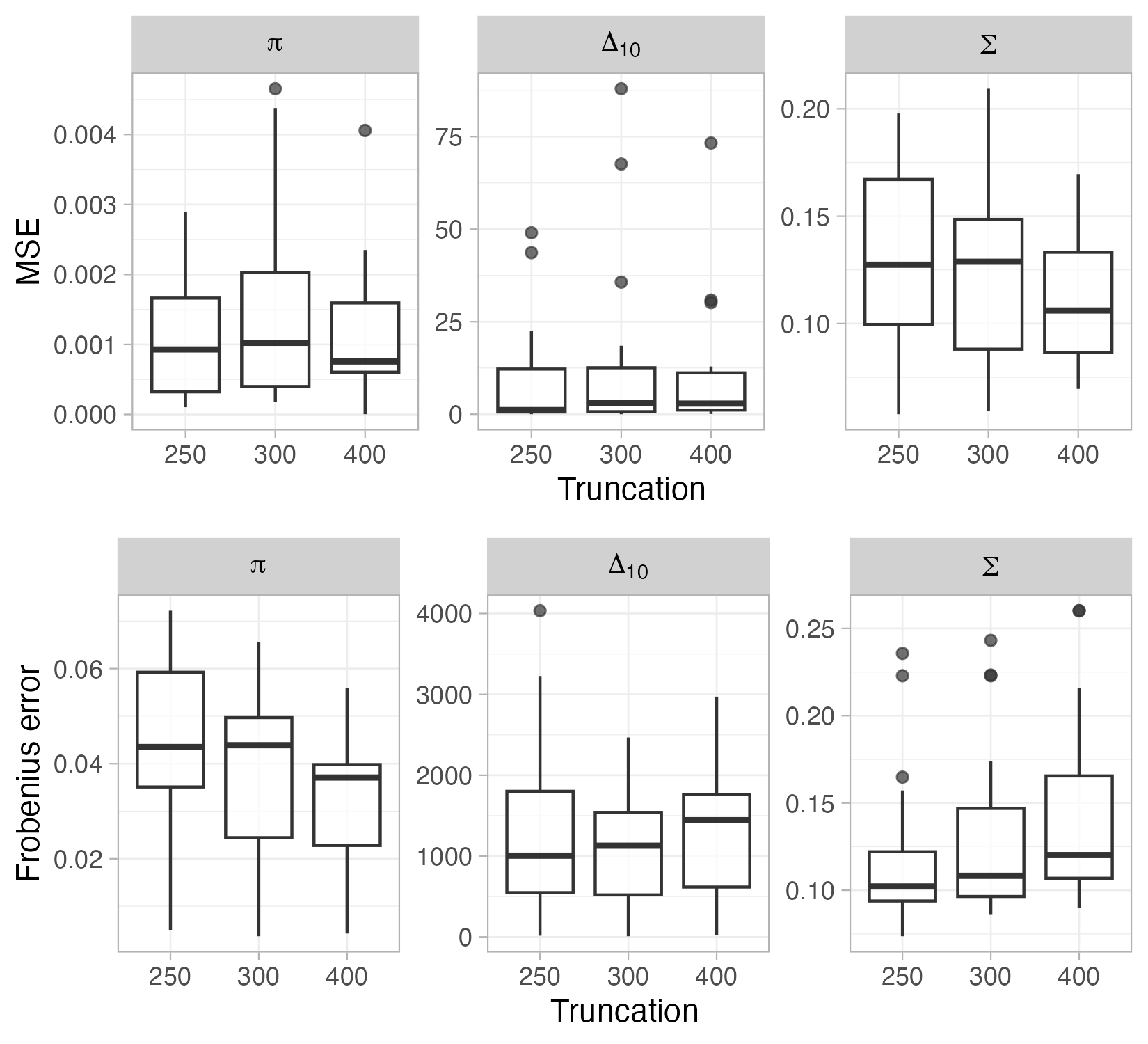
Figure S2: The top panel shows the performance in terms of mean square error for $\bm{\pi}^{*}$, $\bm{\Sigma}^{*}$ and $\Delta_{10}^{*}$ of the factor MVP-IBP in 20 simulations for different truncation levels. The bottom panel shows the performance in terms of Frobenius error for $\bm{\pi}^{*}$, $\bm{\Sigma}^{*}$ and $\Delta_{10}^{*}$ of the hierarchical MVP-IBP in 20 simulations for different truncation levels.

Initialize ($\bm{\gamma}$,$\bm{\Psi}$).

1. Given ($\bm{\gamma}$,$\bm{\Psi}$) obtain approximation to $\Pi(\bm{b}_{j}\mid y,\bm{\gamma},\bm{\Psi})$ as $N(\hat{b}_{j},\bm{Q}_{j})$ for $j=1,\dots,P$ with the prior $\bm{b}_{j}\sim N_{q}(\bm{\gamma},\bm{\Psi}$).

2. Update ($\bm{\gamma},\bm{\Psi})\sim\textrm{NIW}(\bm{\gamma}_{q},\iota_{q},d_{q},\bm{\Xi}_{q})$, where $\iota_{q}=\iota+q$, $d_{q}=d+q$, $\bar{b}=(\sum_{j=1}^{q}\bm{b}_{j})/q$, $\gamma_{q}=(\iota\gamma_{0}+q\bar{b})/\iota_{q}$, $\bm{S}=\sum_{j=1}^{q}(\bm{b}_{j}-\bar{b})(\bm{b}_{j}-\bar{b})^{\top}$ and $\bm{\Xi}_{q}=\bm{\Xi}+\bm{S}+(\iota q/\iota_{q})\sum_{j=1}^{q}(\bm{b}_{j}-\bm{\gamma}_{0})(\bm{b}_{j}-\bm{\gamma}_{0})^{\top}.$

3. Given $\omega$, obtain approximations to $\Pi(\sigma_{jj^{\prime}}\mid y,\omega)$ as $N(\hat{\sigma}_{jj^{\prime}},s_{jk}^{2})$ for $j<j^{\prime}=1,\dots,P$ with pseudo-priors $\Pi_{j}^{*}(\beta_{j}\mid y)\Pi_{j^{\prime}}^{*}(\beta_{j^{\prime}}\mid y)$.

Repeat steps 1-3 T times to obtain T samples of ($\bm{\gamma}$,$\bm{\Psi}$).

Algorithm 3 Two-stage approximate conditional sampler for the hierarchical covariate-dependent MVP-IBP.

References

- Abramowitz and Stegun (1948) Abramowitz, M. and I. A. Stegun (1948). Handbook of Mathematical Functions with formulas, graphs, and mathematical tables, Volume 55. US Government Printing Office.
- Abrego et al. (2020) Abrego, N., B. Crosier, P. Somervuo, N. Ivanova, A. Abrahamyan, A. Abdi, K. Hämäläinen, K. Junninen, M. Maunula, J. Purhonen, et al. (2020). Fungal communities decline with urbanization - more in air than in soil. The ISME Journal 14(11), 2806–2815.
- Abrego et al. (2018) Abrego, N., V. Norros, P. Halme, P. Somervuo, H. Ali-Kovero, and O. Ovaskainen (2018). Give me a sample of air and I will tell which species are found from your region: Molecular identification of fungi from airborne spore samples. Molecular Ecology Resources 18(3), 511–524.
- Beraha and Griffin (2023) Beraha, M. and J. E. Griffin (2023). Normalised latent measure factor models. Journal of the Royal Statistical Society Series B: Statistical Methodology 85(4), 1247–1270.
- Bhattacharya and Dunson (2011) Bhattacharya, A. and D. B. Dunson (2011). Sparse Bayesian infinite factor models. Biometrika 98(2), 291–306.
- Broderick et al. (2013) Broderick, T., J. Pitman, and M. I. Jordan (2013). Feature allocations, probability functions, and paintboxes. Bayesian Analysis 8, 801–836.
- Camerlenghi et al. (2023) Camerlenghi, F., S. Favaro, L. Masoero, and T. Broderick (2023). Scaled process priors for Bayesian nonparametric estimation of the unseen genetic variation. Journal of the American Statistical Association, to appear.
- Chakraborty et al. (2023) Chakraborty, A., R. Ou, and D. B. Dunson (2023). Bayesian inference on high-dimensional multivariate binary responses. Journal of the American Statistical Association, to appear.
- Chib and Greenberg (1998) Chib, S. and E. Greenberg (1998). Analysis of multivariate probit models. Biometrika 85(2), 347–361.
- Colwell (2009) Colwell, R. K. (2009). Biodiversity: concepts, patterns, and measurement. The Princeton Guide to Ecology 663, 257–263.
- Di Benedetto et al. (2020) Di Benedetto, G., F. Caron, and Y. W. Teh (2020). Non-exchangeable feature allocation models with sublinear growth of the feature sizes. In International Conference on Artificial Intelligence and Statistics, Volume 108, pp. 3208–3218. PMLR.
- Doshi et al. (2009) Doshi, F., K. Miller, J. Van Gael, and Y. W. Teh (2009). Variational inference for the Indian buffet process. In Proceedings of the Twelth International Conference on Artificial Intelligence and Statistics, Volume 5, pp. 137–144. PMLR.
- Drezner and Wesolowsky (1990) Drezner, Z. and G. O. Wesolowsky (1990). On the computation of the bivariate normal integral. Journal of Statistical Computation and Simulation 35(1-2), 101–107.
- Genz (1992) Genz, A. (1992). Numerical computation of multivariate normal probabilities. Journal of Computational and Graphical Statistics 1(2), 141–149.
- Gershman et al. (2014) Gershman, S. J., P. I. Frazier, and D. M. Blei (2014). Distance dependent infinite latent feature models. IEEE Transactions on Pattern Analysis and Machine Intelligence 37(2), 334–345.
- Griffiths and Ghahramani (2011) Griffiths, T. and Z. Ghahramani (2011). The Indian Buffet Process: An Introduction and Review. Journal of Machine Learning Research 12(32), 1185–1224.
- Hager (1989) Hager, W. W. (1989). Updating the inverse of a matrix. SIAM Review 31(2), 221–239.
- Ishwaran and James (2001) Ishwaran, H. and L. F. James (2001). Gibbs sampling methods for stick-breaking priors. Journal of the American Statistical Association 96(453), 161–173.
- Lee et al. (2010) Lee, S., J. Z. Huang, and J. Hu (2010). Sparse logistic principal components analysis for binary data. The Annals of Applied Statistics 4(3), 1579.
- Legramanti et al. (2020) Legramanti, S., D. Durante, and D. B. Dunson (2020). Bayesian cumulative shrinkage for infinite factorizations. Biometrika 107(3), 745–752.
- Lücking et al. (2017) Lücking, R., B. P. Hodkinson, and S. D. Leavitt (2017). The 2016 classification of lichenized fungi in the Ascomycota and Basidiomycota - Approaching one thousand genera. The Bryologist 119(4), 361–416.
- Ondov et al. (2011) Ondov, B. D., N. H. Bergman, and A. M. Phillippy (2011). Interactive metagenomic visualization in a Web browser. BMC Bioinformatics 12(385).
- Ovaskainen et al. (2016) Ovaskainen, O., N. Abrego, P. Halme, and D. B. Dunson (2016). Using latent variable models to identify large networks of species-to-species associations at different spatial scales. Methods in Ecology and Evolution 7(5), 549–555.
- Owen (1980) Owen, D. B. (1980). A table of normal integrals. Communications in Statistics-Simulation and Computation 9(4), 389–419.
- Qin et al. (2020) Qin, J., W. Zhang, S.-B. Zhang, and J.-H. Wang (2020). Similar mycorrhizal fungal communities associated with epiphytic and lithophytic orchids of coelogyne corymbosa. Plant Diversity 42(5), 362–369.
- Somervuo et al. (2016) Somervuo, P., S. Koskela, J. Pennanen, R. Henrik Nilsson, and O. Ovaskainen (2016). Unbiased probabilistic taxonomic classification for dna barcoding. Bioinformatics 32(19), 2920–2927.
- Teh and Gorur (2009) Teh, Y. and D. Gorur (2009). Indian buffet processes with power-law behavior. In Advances in Neural Information Processing Systems, Volume 22. Curran Associates, Inc.
- Tikhonov et al. (2020) Tikhonov, G., O. H. Opedal, N. Abrego, A. Lehikoinen, M. M. J. de Jonge, J. Oksanen, and O. Ovaskainen (2020). Joint species distribution modelling with the r-package Hmsc. Methods in Ecology and Evolution 11(3), 442–447.
- Warr et al. (2022) Warr, R. L., D. B. Dahl, J. M. Meyer, and A. Lui (2022). The attraction Indian buffet distribution. Bayesian Analysis 17(3), 931–967.
- Williamson et al. (2010) Williamson, S., P. Orbanz, and Z. Ghahramani (2010). Dependent Indian buffet processes. In Proceedings of the Thirteenth International Conference on Artificial Intelligence and Statistics, Volume 9, pp. 924–931.
- Zhao et al. (2021) Zhao, X., G. Plata, and P. D. Dixit (2021). SiGMoiD: A super-statistical generative model for binary data. PLoS Computational Biology 17(8), e1009275.
- Zhou et al. (2011) Zhou, M., H. Yang, G. Sapiro, D. B. Dunson, and L. Carin (2011). Dependent hierarchical beta process for image interpolation and denoising. In Proceedings of the Fourteenth International Conference on Artificial Intelligence and Statistics, pp. 883–891. JMLR Workshop and Conference Proceedings.
- Zito et al. (2023) Zito, A., T. Rigon, O. Ovaskainen, and D. B. Dunson (2023). Bayesian modeling of sequential discoveries. Journal of the American Statistical Association 118(544), 2521–2532.