FIDLAR: Forecast-Informed Deep Learning Architecture for Flood Mitigation

Abstract

In coastal river systems, frequent floods, often occurring during major storms or king tides, pose a severe threat to lives and property. However, these floods can be mitigated or even prevented by strategically releasing water before extreme weather events with hydraulic structures such as dams, gates, pumps, and reservoirs. A standard approach used by local water management agencies is the “rule-based” method, which specifies predetermined pre-releases of water based on historical and time-tested human experience, but which tends to result in excess or inadequate water release. The model predictive control (MPC), a physics-based model for prediction, is an alternative approach, albeit involving computationally intensive calculations. In this paper, we propose a Forecast Informed Deep Learning Architecture, FIDLAr, to achieve rapid and optimal flood management with precise water pre-releases. FIDLAr seamlessly integrates two neural network modules: one called the Flood Manager, which is responsible for generating water pre-release schedules, and another called the Flood Evaluator, which assesses these generated schedules. The Evaluator module is pre-trained separately, and its gradient-based feedback is used to train the Manager model, ensuring optimal water pre-releases. We have conducted experiments using FIDLAr with data from a flood-prone coastal area in South Florida, particularly susceptible to frequent storms. Results show that FIDLAr is several orders of magnitude faster than currently used physics-based approaches while outperforming baseline methods with improved water pre-release schedules. Our code is at https://github.com/JimengShi/FIDLAR/.

1 Introduction

Floods can result in catastrophic consequences with considerable loss of life Jonkman and Vrijling (2008), huge socio-economic impact Wu et al. (2021), property damage Brody et al. (2007), and environmental devastation Yin et al. (2023a). They pose a threat to food and water security as well as sustainable development Kabir and Hossen (2019). What is even more alarming is that research indicates global climate change may lead to a drastic increase in flood risks in terms of both frequency and scale Wing et al. (2022); Hirabayashi et al. (2013). In coastal areas, flood risks are increasing due to sea-level rise Sadler et al. (2020). Therefore, effective flood management is of utmost importance.

To mitigate flood risks, water management agencies have built controllable hydraulic structures such as dams, gates, pumps, and reservoirs in river systems Kerkez et al. (2016). Determining optimal control schedules of these hydraulic structures is however a challenging problem Bowes et al. (2021). Rule-based methods Bowes et al. (2021); Sadler et al. (2019) formulate control schedules based on insights gained from historically observed data. These schedules are often formalized and extensively documented in databases Marchese et al. (2018). They represent the collective wisdom gathered over decades of experience in managing specific river systems and are commonly adopted by local water management authorities. However, these schedules may expose vulnerabilities during extreme events, which are becoming more likely due to climate change, and might lack sufficient locally available historical data, particularly for events like 500- or 1000-year floods. Moreover, these schedules may not offer effective solutions for complex river systems Schwanenberg et al. (2015).

Model Predictive Control (MPC) is a well-known strategy that tackles this challenge as an optimization process Karimanzira (2016). By optimizing variables such as water levels and discharges, the algorithm generates control schedules for hydraulic structures to effectively mitigate overall flood risks Delaney et al. (2020); Zarei et al. (2021). Random initialization followed by soft-computing techniques such as genetic algorithms is often employed to perform the optimizations. Subsequently, physics-based models such as HEC-RAS and SWMM are used to assess the generated control schedules. Publications on this topic include the following Leon et al. (2020); Sadler et al. (2019); Vermuyten et al. (2018); Chen et al. (2016); Leon et al. (2014); Yin et al. (2023b). However, such MPC methods are prohibitively slow since they require thousands of simulations using physics-based models.

In the last decade or so, Machine learning (ML) has emerged as a powerful tool in this domain. So far, the ML-based methods have been applied to flood prediction Mosavi et al. (2018); Shi et al. (2023b), flood detection Tanim et al. (2022); Shahabi et al. (2020), susceptibility assessment Saha et al. (2021); Islam et al. (2021), and post-flood management Munawar et al. (2019). However, ML-based methods have not been applied to flood mitigation tasks. We aim to fill this gap. Moreover, we replace the compute-intensive MPC approach with a framework based purely on deep learning (DL), where both the generator and evaluator are achieved by DL modules.

Gradient-based planning with world models aims to seek optimal actions by training a world model and conducting inferences using that trained model. We refer the reader to Figure 1(a) from Jyothir et al. (2023).

Figure 1: Forecast-Informed Deep Learning Architecture (FIDLAr). Input data in the form of a table consisting of five variables as shown in the left end of the diagram. The variables $w$ and $k$ are the lengths of the past and prediction windows, respectively. The parts of the table colored green are provided as inputs to the programs, while the orange and blue parts (with question marks) are outputs. The black and red arrows represent the propagation and back-propagation processes, respectively. The Flood Manager and Flood Evaluator represent DL models, the former to predict the control schedules of gates and pumps to pre-release water, and the latter to determine water levels for those control schedules. Loss functions, $\mathcal{L}_{1}$ and $\mathcal{L}_{2}$, penalize the flooding and water wastage beyond pre-specified thresholds, respectively.

Our proposed Forecast Informed Deep Learning Architecture, FIDLAr, uses gradient-based planning to achieve optimal flood management with rapid and feasible water pre-releasing. See Figure 1 for details on its architecture. FIDLAr’s characteristics are summarized as follows:

• FIDLAr seamlessly combines two DL models in series: Flood Manager and Flood Evaluator. The former model is responsible for generating water pre-release schedules, while the latter model accurately forecasts the resulting water levels. The latter model serves as an evaluator for the output of the former. During training, the gradient feedback from the Evaluator model can be back-propagated to reinforce the Manager model to generate effective water pre-release schedules. The Manager and Evaluator play the role of Planner and World Model, respectively, from the model from Jyothir et al. (2023).

• FIDLAr is a data-driven approach, learning flood mitigation strategies from historically observed data. Once trained, it offers rapid response capabilities. This highlights the advantages of DL-based models over physics-based models, particularly in the context of real-time flood management.

• FIDLAr is a model-agnostic framework, where both the Manager and Evaluator could be any type of DL model with differentiable loss functions that allow back-propagation.

• FIDLAr is trained with a custom loss function to balance both flood risks and water wastage at the same time, which is a multitask learning method.

• FIDLAr makes effective use of reliable forecasts of specific variables (e.g., precipitation and tidal information) for the near future.

• The explainability features of FIDLAr allow us to better understand the behavior of complex river systems.

2 Problem Formulation

Flood mitigation involves the prediction of control schedules for hydraulic structures like gates and pumps within the river system, denoted as $X^{gate,pump}_{t+1:t+k}$, spanning $k$ time points from $t+1$ to $t+k$ into the future. This prediction uses as input historical input data (on all variables), $X$, from the preceding $w$ time points, in conjunction with reliably forecasted covariates (such as rainfall and tide) for the next $k$ time points. Thus, we train a DL model whose transfer function, $\mathcal{F}_{\theta}$, has the form:

$$\mathcal{F}_{\theta}:(X_{t-w+1:t},X^{cov}_{t+1:t+k})\rightarrow X^{gate,pump}_{t+1:t+k},$$ (1)

where the subscripts represent the time ranges, and the superscripts refer to the variables under consideration. Superscripts are dropped when all variables are taken into account. The superscript $cov$ refers specifically to the reliably predicted covariates (e.g., rain, tides).

3 Methodology

3.1 The Challenge

Intuitively, an ML model can be trained to learn the function $f_{\theta}$. However, the challenge here is that the historical data may not represent the desired values for the control schedules of the gates and pumps, especially if it resulted in flood conditions, and therefore cannot be used as the ground-truth values used in traditional supervised learning. Therefore, we separate a “planner” (Flood Manager) module from an “evaluator” (Flood Evaluator) module. We first build an independent and accurate evaluator with the historical data, which attempts to learn the consequences of every possible action. We then treat the planner module design as an optimization problem where we optimize a custom loss function, allowing the system to pick the action that would prevent undesirable consequences. Desired states of the river systems avoid floods on one hand while preventing water wastage on the other. Once the Flood Evaluator is trained, it is frozen and used to train the Flood Manager. The evaluator serves to backpropagate the gradient feedback regarding the quality of the schedules generated by the manager, thus guiding the manager to generate more effective schedules of gates and pumps. Such a training process ends up refining the function, $f_{\theta}$, as represented in Eq. (1).

Figure 2: Flood Evaluator. Unlike Figure 1, the parts shaded green (includes historical data and covariates predicted from near future) and orange (representing any control schedule for the gates and pumps) are both used as inputs. Water levels (blue) are the outputs.

3.2 Flood Evaluator

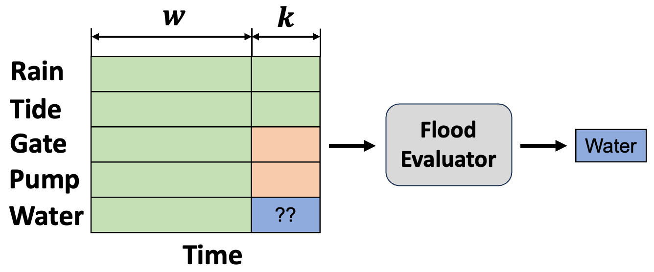
Flood Evaluator is tasked with accurately forecasting water levels at designated points of interest within river systems for any control schedule of gates and pumps provided to it. See Figure 2. The underlying transfer function of the Evaluator has the form:

$$\mathcal{G}_{\theta}:(X_{t-w+1:t},X^{cov}_{t+1:t+k},X^{gate,pump}_{t+1:t+k})\rightarrow X^{water}_{t+1:t+k}.$$ (2)

As mentioned earlier, the Evaluator module is trained independently using the historical data to achieve highly accurate water level predictions for any given set of conditions and control schedules. Therefore, once the Evaluator is trained, its parameters are set in stone for the training of the Manager, where it plays the role of a trained “referee”.

Figure 3: Flood Manager. As in Figure 1, the parts shaded green (historical data) are the inputs, and the parts shaded orange are the outputs. The water levels shaded blue are not predicted.

3.3 Flood Manager

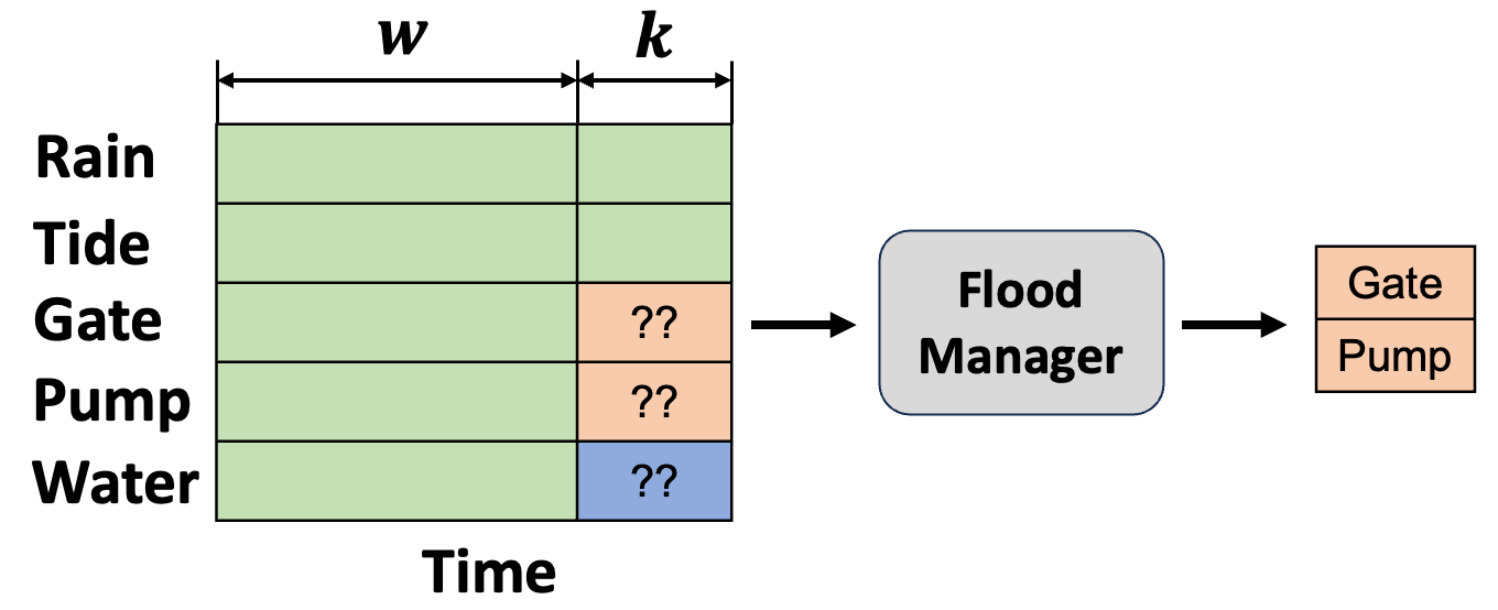
As shown in Figure 3, the Flood Manager is trained to produce optimal control schedules for the hydraulic structures (gates and pumps), taking reliably predictable future information (rain, tide) and all historical data. During its training, since no ground truth is available, it is trained using the gradient descent algorithm Ruder (2016); Andrychowicz et al. (2016), using the partial derivatives of the loss function (Eq. (3)), which in turn needs the evaluator.

3.4 Custom Loss Function

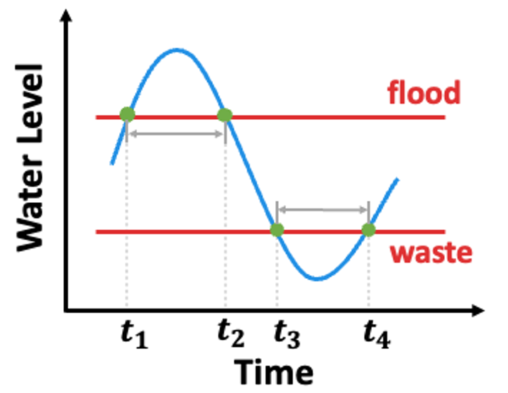
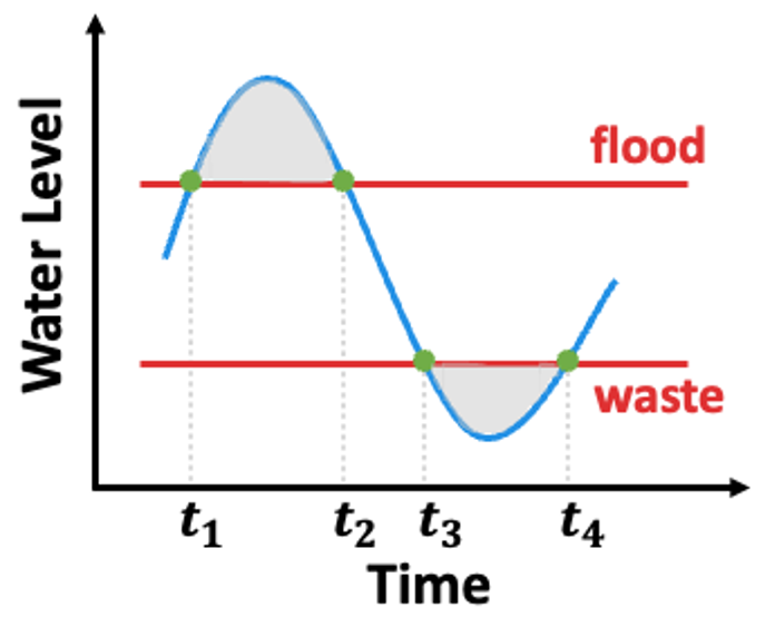
Loss functions are critical in steering the learning process. For flood management, since no ground truth is available, independent metrics of performance are needed. An obvious one is the total time (Figure 4 (a)) for which the water levels either exceed the flooding threshold or dip below the water wastage threshold. Another related metric is the extent to which the limits are exceeded to signify the severity of floods or water wastage (Figure 4 (b)). The lower threshold for flood management is important in practice, since it prevents water wastage, thereby supporting irrigation, facilitating navigation, and maintaining ecological balance. It also prevents the optimization methods from trivially recommending the depletion of valuable water resources to prevent future flooding. The above metrics suggest the following components for the loss function for our models. The final loss function is a balanced combination of $\mathcal{L}_{1}$ and $\mathcal{L}_{2}$ in Eq. (4).

$$\mathcal{L}_{1}=\sum^{N}_{i=1}\sum^{t+k}_{j=t+1}\Arrowvert max\{\hat{X}^{water}_{i,j}-X^{flood}_{i},0\}\Arrowvert^{2},$$ (3)

$$\mathcal{L}_{2}=\sum^{N}_{i=1}\sum^{t+k}_{j=t+1}\Arrowvert min\{\hat{X}^{water}_{i,j}-X^{waste}_{i},0\}\Arrowvert^{2},$$

where $N$ is the number of water level locations of interest; $k$ is the length of prediction horizon; $X^{flood}$ and $X^{waste}$ represent the thresholds for flooding and water wastage; and their capped versions, $\hat{X}^{flood}$ and $\hat{X}^{waste}$ are obtained using the evaluator module. The combined loss function is given by:

$$\mathcal{L}_{total}=\alpha\cdot\mathcal{L}_{1}+\beta\cdot\mathcal{L}_{2},$$ (4)

where $\alpha/\beta$ dictates the relative importance of $\mathcal{L}_{1}$ and $\mathcal{L}_{2}$.

(a)

(b)

Figure 4: The two red bars represent an upper threshold of flooding and a lower threshold of wastage. Shown are (a) the time spans when these thresholds are crossed, and (b) the areas between the water level curve and the threshold bars. Violations of the upper (lower, resp.) threshold are captured in $\mathcal{L}_{1}$ ($\mathcal{L}_{2}$, resp.).

Figure 5: Architecture of Graph Transformer Network for Flood Evaluator. Input variables include Rainfall, Pump, Gate, Tide, and Water levels as shown in Figure 6 and Table 1, which are generically denoted by $R,T,G,P$, and $W$. Output is water levels. We use the same architecture for Evaluator and Manager, but with minor changes accordingly of the input and output(see Figs. 2 and 3).

3.5 Training FIDLAr

The entire training process is outlined below. The Evaluator model is trained in a traditional way using the observed historical data as the ground truth for predictions and minimizing a loss function that penalizes deviations from the ground truth. After the Evaluator model is trained, its parameters are frozen and the Manager model is trained. For every control schedule that the Manager generates, $X^{gate,pump}_{t+1:t+k}$, the Evaluator is used to compute the resulting water levels, which is then used to compute the loss function defined in Eq. (4). Gradient descent Ruder (2016) provides the information to be back-propagated to be used to update the parameters of Manager. Thus,

$${X^{*}}^{gate,pump}_{t+1:t+k}=\underset{X^{gate,pump}_{t+1:t+k}}{\arg\min}\{\mathcal{L}_{total}\}.\\$$ (5)

The training details of FIDLAr are given in Algorithm 1.

4 GTN Model

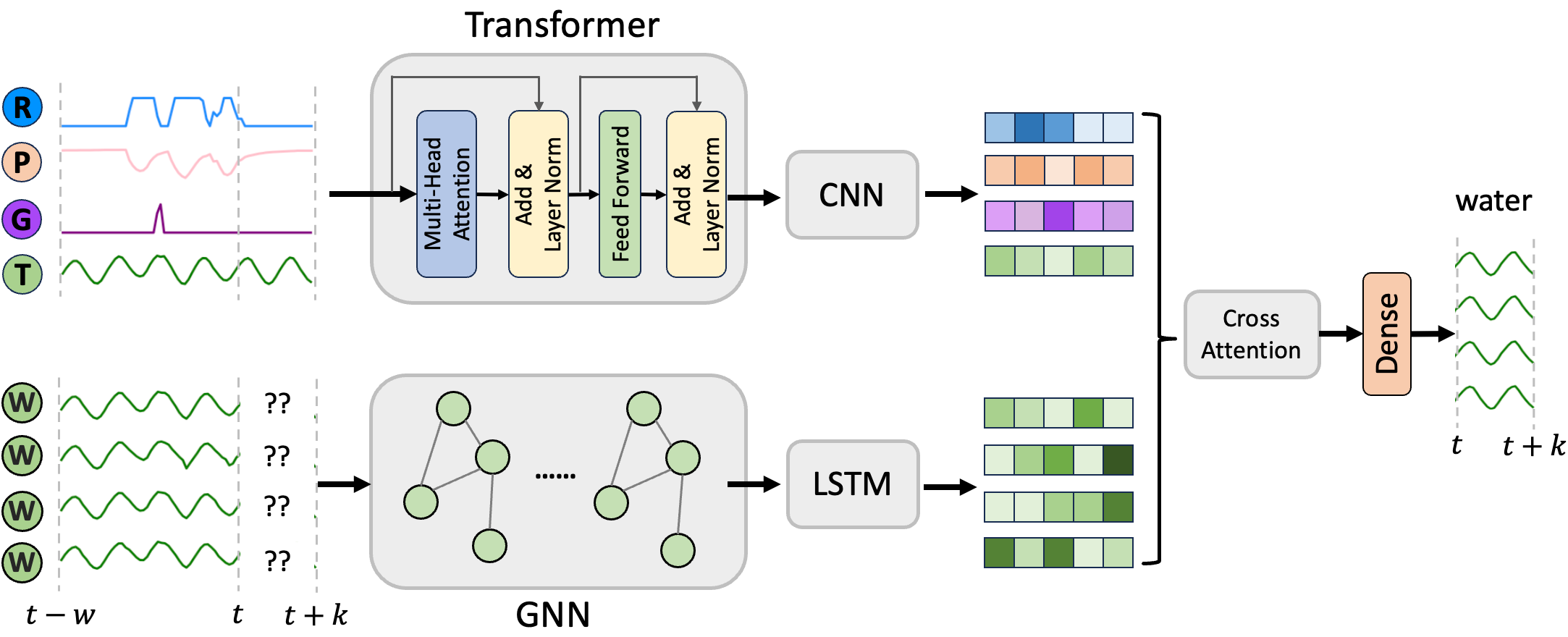
The Manager and Evaluator modules described so far are model agnostic. We tried many existing architectures for them, as discussed in Section 5.2. The Graph Transformer Network (GTN) architecture combines graph neural networks (GNNs), attention-based transformer networks, long short-term memory networks (LSTMs), and the convolutional neural networks (CNNs). GNN and LSTM modules are combined for learning the spatiotemporal dynamics of water levels, while the Transformer and CNN modules focus on extracting feature representations from the covariates. The Attention mechanism is employed to discern the interactions between covariates and water levels, as shown in Eq. (6) below. Figure 5 presents the GTN architecture used (with minor modifications) for the Evaluator and the Manager.

$$Atte(Q,K,V){} =softmax(\frac{Q^{cov}(K^{water})^{T}}{\sqrt{d_{k}}})V^{water}$$ (6)

$$=softmax(\frac{Q^{water}(K^{cov})^{T}}{\sqrt{d_{k}}})V^{cov},$$

where $T$ denotes the transpose operation; $water$ and $cov$ represent the variables of water levels and covariates.

Algorithm 1 Training algorithm of FIDLAr

Input: recent past data: ${\bf X}_{t-w+1,t}$
Input: near future data: ${\bf X}^{cov}_{t+1,t+k}={\bf X}^{rain,tide,gate,pump}_{t+1,t+k}$
Parameter: $\theta_{E},\theta_{M}$: parameters of Evaluator and Manager
Parameter: $w,k:$ length of past and prediction windows

1:  // Train Flood Evaluator, $\mathcal{G}_{\theta_{E}}$

2:  initialize learnable parameters $\theta_{E}$

3:  for $i=1,\ldots,N$ epochs do

4:     $\text{MiniBatch}\leftarrow(\{{\bf X}_{t-w+1,t},{\bf X}^{cov}_{t+1,t+k}\},{\bf X}^{water}_{t+1,t+k})$

5:     $\hat{{\bf X}}^{water}_{t+1,t+k}\leftarrow\mathcal{G}_{\theta_{E}}({\bf X}_{t-w+1,t},{\bf X}^{cov}_{t+1,t+k})$

6:     $\mathcal{L}_{E}\leftarrow\frac{1}{k}\sum_{j=1}^{k}||\hat{{\bf X}}^{water}_{j}-{\bf X}^{water}_{j}||^{2}$

7:     $\nabla_{\theta_{E}}\leftarrow\text{BackwardAD}(\mathcal{L}_{E})$

8:     $\theta_{E}\leftarrow\theta_{E}-\eta\nabla_{\theta_{E}}$

9:  end for

10:  return trained Flood Evaluator, $\mathcal{G}_{\theta_{E}}$

11:  // Train Flood Manager, $\mathcal{F}_{\theta_{M}}$, with frozen $\mathcal{G}_{\theta_{E}}$

12:  initialize learnable parameters $\theta_{M}$

13:  while $X^{water}_{t,t+k}$ violates either threshold do

14:     $\text{MiniBatch}\leftarrow(\{{\bf X}_{t-w+1,t},{\bf X}^{rain,tide}_{t+1,t+k}\},{\bf X}^{gate,pump}_{t+1,t+k})$

15:     $\hat{{\bf X}}^{gate,pump}_{t+1,t+k}\leftarrow\mathcal{F}_{\theta_{M}}({\bf X}_{t-w+1,t},{\bf X}^{rain,tide}_{t+1,t+k})$

16:     $\hat{{\bf X}}^{water}_{t+1,t+k}\leftarrow\mathcal{G}_{\theta_{E}}({\bf X}_{t-w+1,t},{\bf X}^{rain,tide}_{t+1,t+k},\hat{{\bf X}}^{gate,pump}_{t+1,t+k})$

17:     $\mathcal{L}_{E}=\alpha\cdot\mathcal{L}_{1}(\hat{{\bf X}}^{water}_{t+1,t+k})+\beta\cdot\mathcal{L}_{2}(\hat{{\bf X}}^{water}_{t+1,t+k})$

18:     $\nabla_{\theta_{M}}\leftarrow\text{BackwardAD}(\mathcal{L}_{E})$

19:     $\theta_{M}\leftarrow\theta_{M}-\eta\nabla_{\theta_{M}}$

20:  end while

21:  return trained Flood Manager, $\mathcal{F}_{\theta_{M}}$

5 Experiments

5.1 Data

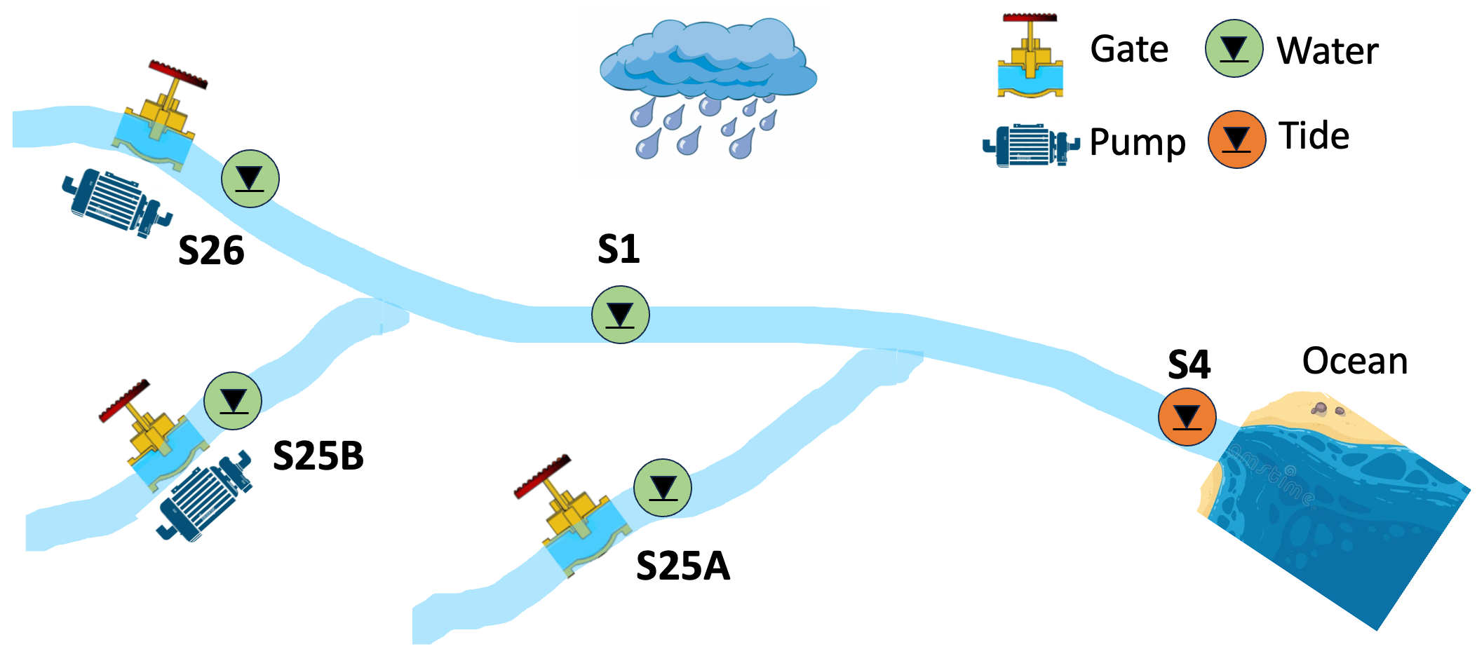
We obtained data from the South Florida Water Management District’s (SFWMD) DBHydro database District (2023) for the coastal stretch of the South Florida watershed. The data set consists of hourly observations for water levels and external covariates from Jan. 1st, 2010 to Dec. 31, 2020, a period totaling eleven years. As shown in Figure 6, the river system under consideration has two branches and includes several hydraulic structures (gates, pumps) to control water flows. Water levels in coastal systems are also impacted by tides. We aim to predict effective schedules on hydraulic structures (gates, pumps) to minimize flood risks at four specific locations marked by green circles in Figure 6. To highlight the risk posed by floods, we note that this portion of the river system flows through Miami downtown, with a sizable population, many commercial enterprises, and an international airport in its vicinity.

Figure 6: Schemetic diagram of study domain - South Florida. There are three water stations with hydraulic structures (S26, S25B, S25A), one simple water station, S1 (green circle in the middle), and one station monitoring tide information from the ocean.

Table 1: Summary of the data set (Jan. 1, 2010 $\sim$ Dec. 31, 2020).

Feature	Interval	Unit	#Var.	Location
Rainfall	Hourly	$inch/h$	1	-
Tide	Hourly	$ft$	1	S4
Pump	Hourly	$ft^{3}/s$	2	S25B, S26
Gate	Hourly	$ft$	3	S25A, S25B, S26
Water	Hourly	$ft$	4	S25A, S25B, S26, S1

5.2 Experimental designs

The sliding input window Li et al. (2014) (also known as look-back window Gidea and Katz (2018) strategy was used to process the entire dataset Shi et al. (2023a)), which helps to ensure that the input and output vector lengths are constant. The datasets were split in chronological order with the first 80% for training and the remaining 20% for testing.

Flood Prediction.

The primary role of the Flood Evaluator is to forecast flood events by predicting water levels for given input conditions. To assess its performance, we compared several DL models for the evaluation, including our proposed GTN model as well as a physics-based model (HEC-RAS). We measured accuracy using multiple metrics: (a) the mean absolute error (MAE), (b) the root mean square error (RMSE) computed between the predicted and actual water levels, (c) the number of time points where the upper or lower thresholds were breached, and (d) the area between the water level curve and the threshold bars. For consistency, we used a look-back window of length $w=72$ hours and a prediction window of length $k=24$ hours. The eight DL methods used are listed below (more details in Appendix B):

• MLP Suykens et al. (1995): Multilayer perceptron can learn complex non-linear dependencies;

• RNN Medsker and Jain (2001): Recurrent neural networks are good at processing sequential data;

• CNN O’Shea and Nash (2015): A 1D convolutional neural network;

• GNN Kipf and Welling (2016): Graph neural network with nodes representing variables and edges representing spatial dependencies;

• TCN Bai et al. (2018): Temporal dilated convolutional network with an exponentially large receptive field;

• RCNN Zhang and Dong (2020): Combined RNN and CNN model for time series forecasting;

• Transformer Vaswani et al. (2017): Attention-based network for sequence modeling (only encoder);

• GTN: Combining GNNs with LSTMs, CNNs, and transformers, as described in Figure 5.

Flood Mitigation with FIDLAr.

FIDLAr requires both Evaluator and Manager components and we chose the GTN model for the Evaluator, since it was the best performing model. For the Manager model, we experimented with one rule-based method, and two genetic algorithms – one with a physics-based HEC-RAS evaluator Leon et al. (2020) and one with our DL-based GTN evaluator, and several DL-based managers. As shown in Table 3, the list of DL approaches used in our experiments for the Manager included MLP, RNN, CNN, GNN, TCN, RCNN, Transformer, and GTN. Performance of FIDLAr was measured using (a) the number of time steps where the upper/lower thresholds were exceeded for the water levels, and (b) the area between the water level curve and the threshold bars.

5.3 Analysis of computational time

Since FIDLAr was designed for real-time flood control, we measured the running times of the models used in this work.

Table 2: Comparison of model performances for the Flood Evaluator on the test set, specifically at time t+1 for measurement station S1. The terms “Over Timesteps” and “Under Timesteps” indicate the number of time steps during which water levels exceed the upper threshold or fall below the lower threshold, respectively. Similarly, “Over Area” and “Under Area” pertain to the area between the water level curve and upper or lower threshold, as was illustrated in Figure 4. Results in red are lowest in that column or closest to the ground truth (in blue).

Methods	MAE (ft)	RMSE (ft)	Over Timesteps	Over Area	Under Timesteps	Under Area
Ground-truth	-	-	96	14.82	1,346	385.80
HEC-RAS	0.174	0.222	68	10.07	1,133	325.33
MLP	0.065	0.086	147	27.96	1,677	500.41
RNN	0.054	0.072	110	17.12	1,527	441.41
CNN	0.079	0.104	58	5.91	1,491	413.22
GNN	0.054	0.070	102	15.90	1,569	462.63
TCN	0.050	0.065	47	5.14	1,607	453.63
RCNN	0.092	0.110	37	4.61	1,829	553.20
Transformer	0.050	0.066	151	25.95	1,513	434.13
GTN (ours)	0.040	0.056	100	15.64	1,390	398.84

Table 3: Comparison of model performances for the Flood Manager on the test set, specifically at time t+1 for measurement station S1. The ^∗ denotes that the GA method was used with a physics-based (HEC-RAS) evaluator. The $-$ denotes that the experiments were timed out. The ^† denotes that the GA method was used with the GTN as the evaluator. All other rows are DL-based flood managers with a DL-based GTN as the evaluator. Results in red font are the best in that column.

Method	Manager	Over Timesteps	Over Area	Under Timesteps	Under Area
Rule-based		96	14.82	1,346	385.8
GA-based	Genetic Algorithm∗ (GA)	-	-	-	-
	Genetic Algorithm† (GA)	86	16.54	454	104
DL-based	MLP	91	13.31	1,071	268.35
	RNN	35	3.97	351	61.05
	CNN	81	11.22	1,163	314.37
	GNN	31	3.72	429	84.31
	TCN	39	3.77	306	55.12
	RCNN	29	3.28	328	58.68
	Transformer	85	11.54	1,180	310.16
	GTN (Ours)	22	2.23	299	53.34

6 Experimental Results

6.1 Flood Prediction

To evaluate the accuracy of the Flood Evaluator, we test FIDLAr with various DL models on the test set by predicting the water levels $k=24$ hours in advance. Table 2 shows the MAEs and RMSEs for the DL-based models and the physics-based model (HEC-RAS). As discussed earlier, we also analyze the time steps and areas over and under the thresholds. We set the upper threshold (flood level) at 3.5 feet and the lower threshold (wastage level) at 0.0 feet. However, the methods remain consistent for many reasonable choices of threshold values. From Table 2, we note that GTN surpasses the performance of other models with predictions most closely aligned with the ground truth (highlighted in red). More results are provided in Table 8 in Appendix C.1.

6.2 Flood Mitigation

Performance measures.

Table 3 shows that all DL-based methods consistently performed better for site S1 than rule-based and GA-based approaches. Moreover, GTN has the best performance under all four metrics, whether it is to control floods or water wastage. The results for all other measurement sites follow a similar pattern, as shown in Table 9 in Appendix C.2.

Performance visualization.

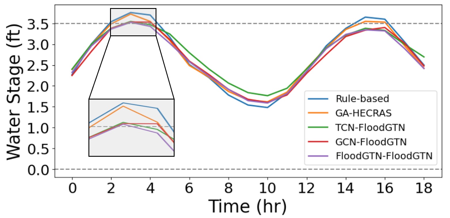
We visualize the mitigated water levels for a short sample spanning 18 hours from September 3rd (09:00) to September 4th (03:00) in 2019 for one location of interest. Figure 7 indicates that FIDLAr equipped with GTN has resulted in water levels within the upper and lower thresholds. The zoomed portion shows a 2.5-hour period where the water levels are decreased under 3.5 feet based on the predicted gate and pump schedules. We provide the corresponding performance in Table 10. More visuals are in Appendix D.

Figure 7: Visualization of water levels with various methods for flood mitigation. We zoomed in the period of $t=2\sim 4.5$ in gray.

6.3 Ablation study

The ablation study quantifies the contribution of each of the components of GTN, by measuring the performance of GTN after removing each of the individual components. Results are shown in Table 4.

Table 4: Ablation study for flood mitigation for the entire test set (for time point t+1 at S1). The last row indicates the performance of the FIDLAr system with GTN as proposed in Figure 5. The best results are in red font.

Removed	Over	Over	Under	Under
Method	Timesteps	Area	Timesteps	Area
CNN	37	4.37	476	85.54
Transformer	32	3.57	325	57.42
GNN	56	5.90	479	86.22
LSTM	35	4.34	329	56.74
Attention	32	3.59	341	60.48
GTN	22	2.23	299	53.34

6.4 Computational time

Table 5 shows the running times for all the methods for the evaluator component and for the whole flood mitigation system in its test phase. All the DL-based approaches are several orders of magnitude faster than the currently used physics-based and GA-based approaches. The table also shows the training times for the DL-based approaches, although they are not necessary for real-time performance.

Table 5: The running time for flood prediction and mitigation. The running time for the rule-based method is not reported since historical data was directly used. GA^∗, which combines a GA-based tool and HEC-RAS, took too long and was not reported although the time for a small data set is reported in Tables 10, 11 in Appendix C.3. GA^†, which combines the GA-based tool with GTN, also took too long but was estimated using a smaller sample.

Model	Prediction		Mitigation
	Train	Test	Train	Test
HEC-RAS	-	45 min	-	-
Rule-based	-	-	-	-
GA∗	-	-	-	-
GA†	-	-	-	est. 30 h
MLP	35 min	1.88 s	58 min	6.13 s
RNN	243 min	8.57 s	54 min	12.75 s
CNN	37 min	1.93 s	17 min	5.84 s
GNN	64 min	3.13 s	29 min	7.26 s
TCN	60 min	4.57 s	45 min	9.06 s
RCNN	136 min	8.61 s	61 min	13.27 s
Transformer	43 min	2.38 s	23 min	6.76 s
GTN	119 min	2.95 s	35 min	4.90 s

6.5 Model explainability

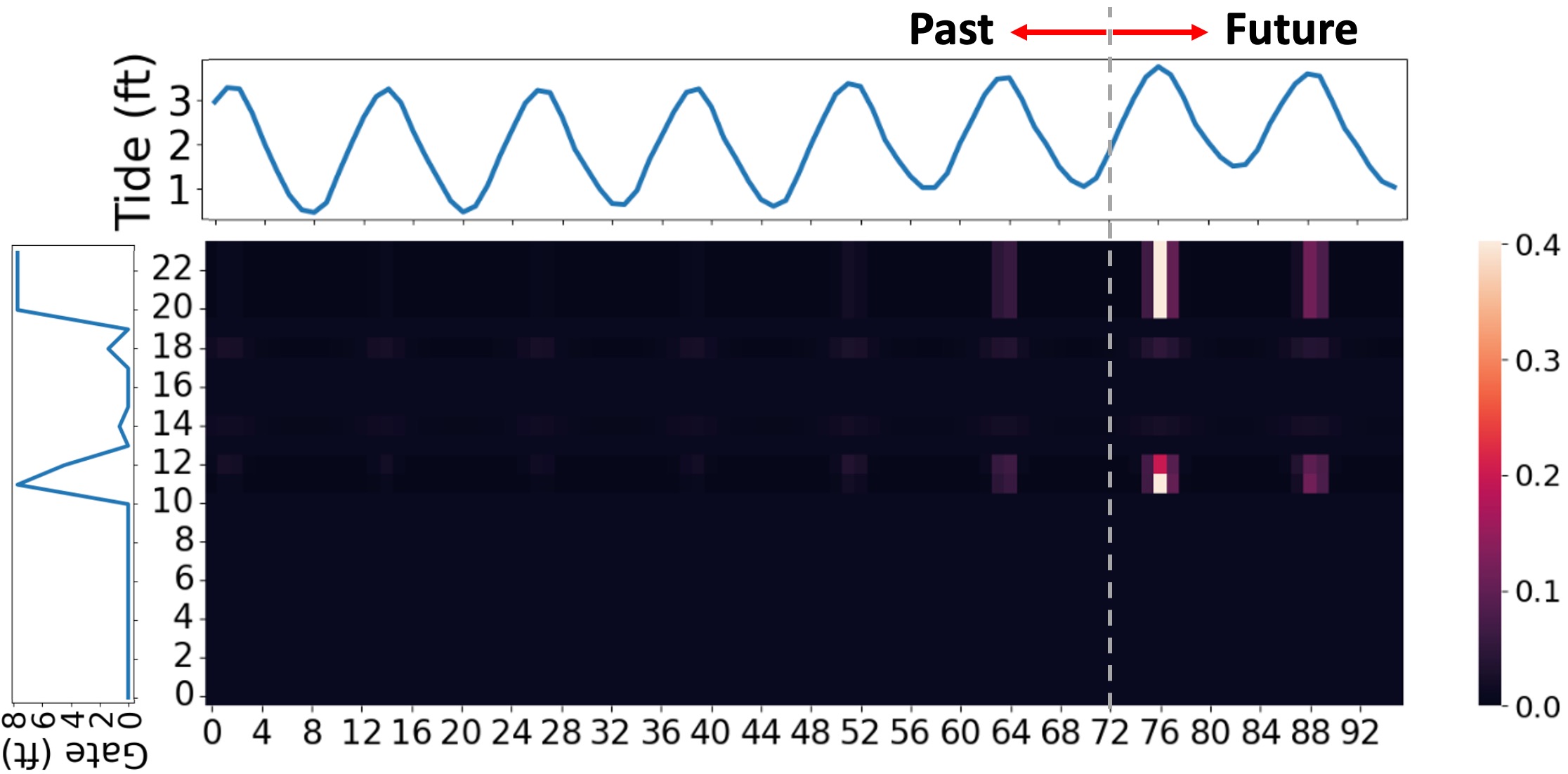
Attention-based methods allow us to calculate the “attention scores” assigned to an input variable to compute a specific output variable. This is exemplified in the heatmap shown in Figure 8, which shows the attention scores assigned to the tide (columns) to compute the gate schedule output (rows) for 24 hours into the future. Note that there are 96 columns and 24 rows because we use 72 hours of past tidal observations and 24 hours of future predicted tidal data to predict 24 hours of the gate schedule into the future. Thus the rows $[0,23]$ correspond to the 24 hours into the future, while the columns $[0,95]$ also include 72 hours of the recent past. Thus, $t=72$ corresponds to the “current” time point, and the columns $[72,95]$ correspond to the same time points as rows $[0,23]$.

Figure 8: Attention scores between tide input and one of the gate schedule outputs. $x$ and $y$ axes are the tide and gate over time.

7 Discussion

Interpreting Attention Map.

The explainability feature, which was shown with an example in Figure 8, can provide significant insights into our results. Firstly, the simple example with the attention paid to the variable “tide” shows that the brightest patches in the heatmap occur in the last 24 columns. This highlights the importance of the novel idea of using tidal forecasting information in our flood mitigation approach. Given that tidal information within a 24-hour window can be quite accurate, this is useful. While tides may have a more predictable pattern over time, the contribution of rain on the water levels can also be seen for other time points. A second critical insight is that the brightest attention patches are in columns where the tide is at its highest is critical to the prediction of gate schedules. Additionally, the water level at the first high tide peak after the “current” time is more significant than the other two. Third, the gate schedule has peaks at times $t=11h$ and $t=22h$ into the future, which correspond to the lowest points of the tide. This implies that the optimal time for pre-releasing water is during low tide phases. Opening gates during high tide periods in coastal river systems is less advisable, as it may lead to water flowing back upstream from the ocean. Finally, we observe that while there is a light patch around column $t=65h$, suggesting mild attention for the previous high tide peak, but almost no attention to any of the peaks prior to that. This again suggests that we could have chosen to use a smaller window for the past input. Doing this analysis for more time points could provide evidence for the right value of $w$, the size of the look-back window.

8 Conclusions

FIDLAr is a DL-based tool to compute water “pre-release” schedules for hydraulic structures in a river system to achieve effective and efficient flood mitigation, while ensuring that water wastage is avoided. This was made possible by the use of well-crafted loss functions for the DL models. The dual component design (with a Manager and an Evaluator) is a strength of FIDLAr. During training, the gradient-based back-propagation from the Evaluator helps to fine-tune the Manager. The reliability of forecasts of variables like precipitation and tides is well known, but their critical importance may have been best demonstrated for the first time using the attention mechanism employed herein.

All the DL-based versions of FIDLAr are several orders of magnitude faster than the (physics-based or GA-based) competitors while achieving improvement over other methods in flood mitigation. These characteristics allow us to entertain the possibility of real-time flood management, which was previously unthinkable.

Appendix A Data and Processing

Data.

We describe more details about the data set used in our work. This dataset includes water level measurements from multiple stations, control schedules for various hydraulic structures (such as gates and pumps) along the river, tide information, and rainfall data in South Florida, USA. We aim to predict effective schedules on hydraulic structures (gates, pumps at S25A, S25B, S26) to minimize flood risks at four specific locations as represented in the green circle in Fig. 6. The relative water stage $\in\text{[-1.25, 4.05]}$ feet. This dataset spans 11 years, ranging from 2010 to 2020, with hourly measurements. The primary feature description and diagram of the study domain are presented in Table 1.

Processing.

Flood Evaluator is used to predict the water levels given the input of past $w$ time steps and some information of future $k$ time steps, either predicted information (“Rain” and “Tide”) or pre-determined information (“Gate” and “Pump”). It serves as an evaluator to assess the gate and pump schedules by predicting the resulting water levels. Flood Manager is used to predict the gate and pump schedules given the input of past $w$ time steps and some information of future $k$ time steps, either predicted information (“Rain” and “Tide”). Both models are trained as supervised learning tasks. Therefore, we pre-processed the data into pairs consisting of the input and output described above. In our experiments, we set $w=72$ hours and $k=24$ hours. The shape of the input and output is $(96,N_{input})$ and $(24,N_{output})$, where $N_{input}$ and $N_{output}$ are the number of input and output variables, respectively. Among the input, the future data with question marks is masked to a $mask\_value=1e-10$ using Keras API. If all values in the input tensor at that time steps are equal to $mask\_value$, then the time steps will be masked (skipped) in all downstream layers.

(a) Flood Evaluator

(b) Flood Manager

Figure 9: Flood Evaluator and Flood Manager in FIDLAR.

Appendix B Model Architecture and Training Hyper-parameter

B.1 Architecture

Since FIDLAR is a model-agnostic framework, we use different deep learning models below as the backbone. In this section, we provide the model architecture, accordingly.

• MLP: We stacked two Dense layers with $64$ and $32$ neurons. Each Dense layer uses RELU as the activation function and $L_{1}$ and $L_{2}$ as the regularization factor. Each Dense layer is followed by a Dropout layer to avoid possible overfitting.

• RNN: We used one SimpleRNN layer with $64$ neurons followed by a Dropout layer. The SimpleRNN layer uses RELU as the activation function and $L_{1}$ and $L_{2}$ as the regularization factor.

• CNN: We stacked three CNN1D layers with $64$, $32$, and $16$ filters, followed by MaxPooling1D layer with pool size $=2$. Each CNN1D layer uses RELU as the activation function, “same” padding mode sand 2 as the kernel size.

• GNN: We consider each time series as one node and the connection as the edge. For the variables in Fig. 6, we assign “1” to the edge between two connected nodes, otherwise, “0”. For the architecture, we stacked two graph convolutional networks (GCNs) with $32$ and $16$ neurons. In parallel, a LSTM layer with $32$ units is used to learn the temporal dynamics from the input. We then concatenate the embedding from GCN and LSTM and output the outcomes.

• TCN: It is a temporal dilated convolutional network with an exponentially large receptive field. We used $64$ as the number of filters, $2$ as the kernel size, $[1,2,4,8,16,32]$ as dilations, and 0.1 as the dropout rate. Subsequently, we added two Dense layers to compute the output. LayerNormalization is employed after each layer.

• RCNN: A SimpleRNN with $64$ neurons, RELU as the activation function and $L_{1}$ and $L_{2}$ as the regularization factor is used first. We then used a CNN1D layer with $32$ filters to deal with the embedding above. The CNN1D layer has 2 as kernel size, “same” padding mode, and RELU as the activation function. MaxPooling1D layer with pool size $=2$ is added after CNN1D layer.

• Transformer: The standard Transformer encoder Vaswani et al. [2017] is used. In our case, we only used 1 Encoder with 1 head. We set head size=128, embedding dimension=64, Dense layer with 32 neurons. Dropout is used after each layer above.

• GTN: We combine the components of GNNs, LSTMs, Transformer, CNNs, and attention, as described in Fig. 5. We have $32$ and $16$ for GNN’s channels, $16$ for LSTM units, $96$ for CNN filters, and one Transformer encoder with $3$ heads (head size=192, embedding dimension=96).
  

Note.

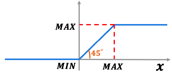
When we used the above models for Flood Evaluator and Flood Manager, the input and output need to be changed accordingly (see Figures 2 and 3). To align with real-world scenarios, we enforce stringent constraints that restrict the output of Manager (values for gate and pump openings) to fall within the range of $[MIN,MAX]$ by a modified RELU activation function in Eq. (7). Fig. 10 provides the corresponding visualization.

$$x=min\{max\{x,MIN\},MAX\},$$ (7)

where $x$ is the opening value of gates and pumps.

Figure 10: Constraint for the values gate and pump openings.

B.2 Training hyper-parameters

In the following table, we show some hyper-parameters used in our experiments: learning rate, batch size, epoch, decay rate, decay step, patience for early stopping, dropout rate, and regularization factors $L_{1}$ and $L_{2}$.

Methods	LR	Batch Size	Epoch	Decay Rate	Decay Step	Patience	Dropout Rate	$L_{1}$	$L_{2}$
MLP	1e-3	512	3000	0.95	10,000	500	0.1	1e-5	1e-5
RNN	1e-4	512	3000	0.95	10,000	500	0.2	1e-5	1e-5
CNN	1e-4	512	3000	0.95	10,000	500	0.1	-	-
GCN	5e-4	512	3000	0.95	10,000	500	0.0	-	-
TCN	5e-4	512	3000	0.95	10,000	500	0.1	-	-
RCNN	1e-4	512	3000	0.95	10,000	500	0.2	0	1e-5
Transformer	5e-4	512	3000	0.95	10,000	500	0.3	-	-
GTN (ours)	5e-4	512	3000	0.95	10,000	500	0.5	1e-5	1e-5

Table 6: Best hyperparameters of each DL model for Flood Evaluator.

Methods	LR	Batch Size	Epoch	Decay Rate	Decay Step	Dropout Rate	Patience	$L_{1}$	$L_{2}$
MLP	1e-3	512	700	0.95	10,000	0.0	100	1e-5	1e-5
RNN	1e-3	512	700	0.95	10,000	0.2	100	1e-5	1e-5
CNN	3e-3	512	700	0.95	10,000	0.0	100	0.0	0.0
GNN	5e-4	512	700	0.9	10,000	0.0	100	0.0	0.0
TCN	1e-3	512	700	0.9	10,000	0.0	100	0.0	0.0
RCNN	1e-3	512	700	0.9	10,000	0.0	100	0.0	1e-5
Transformer	5e-4	512	700	0.9	10,000	0.5	100	0.0	0.0
GTN (ours)	3e-3	512	700	0.95	10,000	0.5	100	1e-5	1e-5

Table 7: Best hyperparameters of each DL model for Flood Manager.

Appendix C More experimental results

C.1 Flood prediction at all locations

In Table 2, we provided the comparison of the performance of different models for the Flood Evaluator at time point $t+1$, but at one location (S1). In Table 8, we provide the comparison of the performance of different models for the Flood Evaluator on the test set at time $t+1$, but for all locations.

Methods	MAE (ft)	RMSE (ft)	Over Timesteps	Over Area	Under Timesteps	Under Area
Ground-truth	-	-	427	68.61	5,116	1465.10
HEC-RAS	0.185	0.238	334	50.85	4,469	1274.26
MLP	0.060	0.080	900	245.75	5,493	1536.22
RNN	0.053	0.071	377	57.32	4,813	1308.28
CNN	0.075	0.105	342	53.69	5,182	1394.05
GCN	0.052	0.069	493	81.28	5,170	1454.78
TCN	0.063	0.097	335	48.37	5,479	1470.41
RCNN	0.121	0.138	288	45.10	5,631	1555.63
Transformer	0.049	0.065	515	85.49	5,046	1372.50
GTN (ours)	0.047	0.064	439	76.01	5,859	1689.45

Table 8: Comparison of different models for the Flood Evaluator on the test set (at time t+1 for all stations). “Over Timesteps” (and “Under Timesteps”) represent the number of time steps during which the water levels exceed the upper threshold (subceed the lower threshold, resp.). Similarly, “Over Area” (and “Under Area”) refer to the area between the water level curve and the upper threshold (lower threshold, resp.), as shown in Fig. 4 in the manuscript.

C.2 Flood mitigation at all locations

In Table 3, we provided the comparison of the performance of different models for the Flood Manager at time point $t+1$, but at one location (S1). We provide the comparison results of different models for the Flood Manager on the test set (at time t+1 for all locations) in Table 9.

Method	Manager	Over Timesteps	Over Area	Under Timesteps	Under Area
Rule-based	-	427	68.61	5,116	1465.10
GA-based	Genetic Algorithm∗ (GA)	-	-	-	-
	Genetic Algorithm† (GA)	343	67.50	1,817	416
DL-based	MLP	435	67.28	3,511	818.06
	RNN	211	25.28	386	58.39
	CNN	372	54.72	3,969	1,044.71
	GCN	181	25.06	1,109	207.48
	TCN	224	25.61	562	92.16
	RCNN	170	20.01	542	88.72
	Transformer	374	54.31	4,378	1,142.98
	GTN‡ (Ours)	114	12.09	617	98.42

Table 9: Comparison of different methods for the Flood Manager on the test set (at time t+1 for all stations). The ^∗ denotes that the GA method was used for Flood Manager with a physics-based (HEC-RAS) as an Evaluator. $-$ denotes too long to get results. The ^† denotes that the GA method was used for Flood Manager with the DL-based GTN as the Evaluator. All other rows are DL-based flood managers with a DL-based GTN as the Evaluator. ^‡ denotes the best.

C.3 Flood mitigation with one event

In Fig. 7, we visualize the results of different models for the Flood Manager on a short event spanning 18 hours from September 3rd (09:00) to September 4th (03:00) in 2019 for one location of interest. Below are the corresponding experiment results.

Method	Manager	Over Timesteps	Over Area	Under Timesteps	Under Area
Rule-based	-	6	0.866	0	0
GA-Based	Genetic Algorithm∗ (GA)	4	0.351	0	0
	Genetic Algorithm† (GA)	6	0.764	0	0
DL-Based	MLP	6	0.614	0	0
	RNN	1	0.074	0	0
	CNN	6	0.592	0	0
	GNN	2	0.062	0	0
	TCN	1	0.046	0	0
	RCNN	1	0.045	0	0
	Transformer	6	0.614	0	0
	GTN‡ (Ours)	1	0.022	0	0

Table 10: Comparison of different methods of Flood Manager for flood Mitigation (at time t+1 for one event S1).

Appendix D Visualization

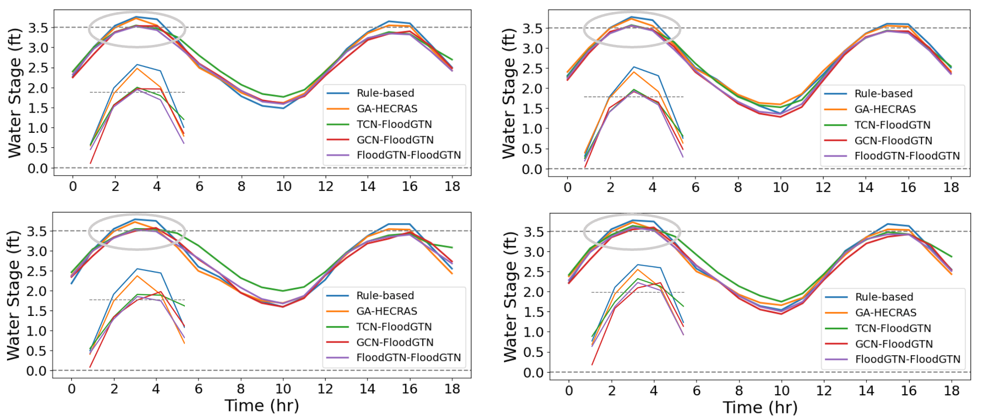
Fig. 11 presents the results for all locations compared to Fig. 7 for one location of interest. Table 11 shows the corresponding performance measures.

Figure 11: Visualization for flood mitigation at all locations. Two gray dashed lines represent the upper (3.5 ft) and lower threshold (0.0 ft).

Method	Manager	Over Timesteps	Over Area	Under Timesteps	Under Area
Rule-based	-	23	3.62	0	0
GA-Based	Genetic Algorithm∗ (GA)	16	1.39	0	0
	Genetic Algorithm† (GA)	23	3.75	0	0
DL-Based	MLP	23	4.18	0	0
	RNN	8	0.63	0	0
	CNN	21	2.92	0	0
	GCN	6	0.32	0	0
	TCN	6	0.39	0	0
	RCNN	6	0.39	0	0
	Transformer	22	3.00	0	0
	GTN‡ (Ours)	5	0.22	0	0

Table 11: Comparison of different methods of Flood Manager for flood Mitigation (at time t+1 for one event at all locations).

References

- Andrychowicz et al. [2016] Marcin Andrychowicz, Misha Denil, Sergio Gomez, Matthew W Hoffman, David Pfau, Tom Schaul, Brendan Shillingford, and Nando De Freitas. Learning to learn by gradient descent by gradient descent. Advances in neural information processing systems, 29, 2016.
- Bai et al. [2018] Shaojie Bai, J Zico Kolter, and Vladlen Koltun. An empirical evaluation of generic convolutional and recurrent networks for sequence modeling. arXiv preprint arXiv:1803.01271, 2018.
- Bowes et al. [2021] Benjamin D Bowes, Arash Tavakoli, Cheng Wang, Arsalan Heydarian, Madhur Behl, Peter A Beling, and Jonathan L Goodall. Flood mitigation in coastal urban catchments using real-time stormwater infrastructure control and reinforcement learning. Journal of Hydroinformatics, 23(3):529–547, 2021.
- Brody et al. [2007] Samuel D Brody, Sammy Zahran, Praveen Maghelal, Himanshu Grover, and Wesley E Highfield. The rising costs of floods: Examining the impact of planning and development decisions on property damage in florida. Journal of the American Planning Association, 73(3):330–345, 2007.
- Chen et al. [2016] Duan Chen, Arturo S Leon, Nathan L Gibson, and Parnian Hosseini. Dimension reduction of decision variables for multireservoir operation: A spectral optimization model. Water Resources Research, 52(1):36–51, 2016.
- Delaney et al. [2020] Chris J Delaney, Robert K Hartman, John Mendoza, Michael Dettinger, Luca Delle Monache, Jay Jasperse, F Martin Ralph, Cary Talbot, James Brown, David Reynolds, et al. Forecast informed reservoir operations using ensemble streamflow predictions for a multipurpose reservoir in northern california. Water Resources Research, 56(9):e2019WR026604, 2020.
- District [2023] South Florida Water Management District. Dbhydro of south florida water management district. https://www.sfwmd.gov/science-data/dbhydro, 2023.
- Gidea and Katz [2018] Marian Gidea and Yuri Katz. Topological data analysis of financial time series: Landscapes of crashes. Physica A: Statistical Mechanics and its Applications, 491:820–834, 2018.
- Hirabayashi et al. [2013] Yukiko Hirabayashi, Roobavannan Mahendran, Sujan Koirala, Lisako Konoshima, Dai Yamazaki, Satoshi Watanabe, Hyungjun Kim, and Shinjiro Kanae. Global flood risk under climate change. Nature climate change, 3(9):816–821, 2013.
- Islam et al. [2021] Abu Reza Md Towfiqul Islam, Swapan Talukdar, Susanta Mahato, Sonali Kundu, Kutub Uddin Eibek, Quoc Bao Pham, Alban Kuriqi, and Nguyen Thi Thuy Linh. Flood susceptibility modelling using advanced ensemble machine learning models. Geoscience Frontiers, 12(3):101075, 2021.
- Jonkman and Vrijling [2008] Sebastiaan N Jonkman and Johannes K Vrijling. Loss of life due to floods. Journal of Flood Risk Management, 1(1):43–56, 2008.
- Jyothir et al. [2023] SV Jyothir, Siddhartha Jalagam, Yann LeCun, and Vlad Sobal. Gradient-based planning with world models. arXiv preprint arXiv:2312.17227, 2023.
- Kabir and Hossen [2019] Md Humayain Kabir and Md Nazmul Hossen. Impacts of flood and its possible solution in Bangladesh. Disaster Adv, 12(10):48–57, 2019.
- Karimanzira [2016] Divas Karimanzira. Model based decision support systems. Modeling, Control and Optimization of Water Systems: Systems Engineering Methods for Control and Decision Making Tasks, pages 185–220, 2016.
- Kerkez et al. [2016] Branko Kerkez, Cyndee Gruden, Matthew Lewis, Luis Montestruque, Marcus Quigley, Brandon Wong, Alex Bedig, Ruben Kertesz, Tim Braun, Owen Cadwalader, et al. Smarter stormwater systems, 2016.
- Kipf and Welling [2016] Thomas N Kipf and Max Welling. Semi-supervised classification with graph convolutional networks. arXiv preprint arXiv:1609.02907, 2016.
- Leon et al. [2014] Arturo S Leon, Elizabeth A Kanashiro, Rachelle Valverde, and Venkataramana Sridhar. Dynamic framework for intelligent control of river flooding: Case study. Journal of Water Resources Planning and Management, 140(2):258–268, 2014.
- Leon et al. [2020] Arturo S Leon, Yun Tang, Li Qin, and Duan Chen. A MATLAB framework for forecasting optimal flow releases in a multi-storage system for flood control. Environmental Modelling & Software, 125:104618, 2020.
- Li et al. [2014] Lei Li, Farzad Noorian, Duncan JM Moss, and Philip HW Leong. Rolling window time series prediction using MapReduce. In Proceedings of the 2014 IEEE 15th international conference on information reuse and integration (IEEE IRI 2014), pages 757–764. IEEE, 2014.
- Marchese et al. [2018] Dayton Marchese, Jeremiah Johnson, Nicholas Akers, Matt Huffman, and Viktor Hlas. Quantitative comparison of active and passive stormwater infrastructure: case study in Beckley, West Virginia. In WEFTEC 2018, pages 4298–4311. Water Environment Federation, 2018.
- Medsker and Jain [2001] Larry R Medsker and LC Jain. Recurrent neural networks. Design and Applications, 5(64-67):2, 2001.
- Mosavi et al. [2018] Amir Mosavi, Pinar Ozturk, and Kwok-wing Chau. Flood prediction using machine learning models: Literature review. Water, 10(11):1536, 2018.
- Munawar et al. [2019] Hafiz Suliman Munawar, Ahmad Hammad, Fahim Ullah, and Tauha Hussain Ali. After the flood: A novel application of image processing and machine learning for post-flood disaster management. In Proceedings of the 2nd International Conference on Sustainable Development in Civil Engineering (ICSDC 2019), Jamshoro, Pakistan, pages 5–7, 2019.
- O’Shea and Nash [2015] Keiron O’Shea and Ryan Nash. An introduction to convolutional neural networks. arXiv preprint arXiv:1511.08458, 2015.
- Ruder [2016] Sebastian Ruder. An overview of gradient descent optimization algorithms. arXiv preprint arXiv:1609.04747, 2016.
- Sadler et al. [2019] Jeffrey M Sadler, Jonathan L Goodall, Madhur Behl, Mohamed M Morsy, Teresa B Culver, and Benjamin D Bowes. Leveraging open source software and parallel computing for model predictive control of urban drainage systems using epa-swmm5. Environmental Modelling & Software, 120:104484, 2019.
- Sadler et al. [2020] Jeffrey M Sadler, Jonathan L Goodall, Madhur Behl, Benjamin D Bowes, and Mohamed M Morsy. Exploring real-time control of stormwater systems for mitigating flood risk due to sea level rise. Journal of Hydrology, 583:124571, 2020.
- Saha et al. [2021] Asish Saha, Subodh Chandra Pal, Alireza Arabameri, Thomas Blaschke, Somayeh Panahi, Indrajit Chowdhuri, Rabin Chakrabortty, Romulus Costache, and Aman Arora. Flood susceptibility assessment using novel ensemble of hyperpipes and support vector regression algorithms. Water, 13(2):241, 2021.
- Schwanenberg et al. [2015] D Schwanenberg, BPJ Becker, and M Xu. The open real-time control (RTC)-tools software framework for modeling RTC in water resources sytems. Journal of Hydroinformatics, 17(1):130–148, 2015.
- Shahabi et al. [2020] Himan Shahabi, Ataollah Shirzadi, Kayvan Ghaderi, Ebrahim Omidvar, Nadhir Al-Ansari, John J Clague, Marten Geertsema, Khabat Khosravi, Ata Amini, Sepideh Bahrami, et al. Flood detection and susceptibility mapping using sentinel-1 remote sensing data and a machine learning approach: Hybrid intelligence of bagging ensemble based on k-nearest neighbor classifier. Remote Sensing, 12(2):266, 2020.
- Shi et al. [2023a] Jimeng Shi, Rukmangadh Myana, Vitalii Stebliankin, Azam Shirali, and Giri Narasimhan. Explainable parallel rcnn with novel feature representation for time series forecasting. arXiv preprint arXiv:2305.04876, 2023.
- Shi et al. [2023b] Jimeng Shi, Zeda Yin, Rukmangadh Myana, Khandker Ishtiaq, Anupama John, Jayantha Obeysekera, Arturo Leon, and Giri Narasimhan. Deep learning models for water stage predictions in south florida. arXiv preprint arXiv:2306.15907, 2023.
- Suykens et al. [1995] Johan AK Suykens, Joos PL Vandewalle, and Bart L De Moor. Artificial neural networks for modelling and control of non-linear systems. Springer Science & Business Media, 1995.
- Tanim et al. [2022] Ahad Hasan Tanim, Callum Blake McRae, Hassan Tavakol-Davani, and Erfan Goharian. Flood detection in urban areas using satellite imagery and machine learning. Water, 14(7):1140, 2022.
- Vaswani et al. [2017] Ashish Vaswani, Noam Shazeer, Niki Parmar, Jakob Uszkoreit, Llion Jones, Aidan N Gomez, Łukasz Kaiser, and Illia Polosukhin. Attention is all you need. Advances in neural information processing systems, 30, 2017.
- Vermuyten et al. [2018] Evert Vermuyten, Pieter Meert, Vincent Wolfs, and Patrick Willems. Combining model predictive control with a reduced genetic algorithm for real-time flood control. Journal of Water Resources Planning and Management, 144(2):04017083, 2018.
- Wing et al. [2022] Oliver EJ Wing, William Lehman, Paul D Bates, Christopher C Sampson, Niall Quinn, Andrew M Smith, Jeffrey C Neal, Jeremy R Porter, and Carolyn Kousky. Inequitable patterns of us flood risk in the anthropocene. Nature Climate Change, 12(2):156–162, 2022.
- Wu et al. [2021] Xianhua Wu, Ji Guo, Xianhua Wu, and Ji Guo. A new economic loss assessment system for urban severe rainfall and flooding disasters based on big data fusion. Economic impacts and emergency management of disasters in China, pages 259–287, 2021.
- Yin et al. [2023a] Jie Yin, Yao Gao, Ruishan Chen, Dapeng Yu, Robert Wilby, Nigel Wright, Yong Ge, Jeremy Bricker, Huili Gong, and Mingfu Guan. Flash floods: why are more of them devastating the world’s driest regions? Nature, 615(7951):212–215, 2023.
- Yin et al. [2023b] Zeda Yin, Linglong Bian, Beichao Hu, Jimeng Shi, and Arturo S Leon. Physic-informed neural network approach coupled with boundary conditions for solving 1d steady shallow water equations for riverine system. In World Environmental and Water Resources Congress 2023, pages 280–288, 2023.
- Zarei et al. [2021] Manizhe Zarei, Omid Bozorg-Haddad, Sahar Baghban, Mohammad Delpasand, Erfan Goharian, and Hugo A Loáiciga. Machine-learning algorithms for forecast-informed reservoir operation (FIRO) to reduce flood damages. Scientific reports, 11(1):24295, 2021.
- Zhang and Dong [2020] Zao Zhang and Yuan Dong. Temperature forecasting via convolutional recurrent neural networks based on time-series data. Complexity, 2020:1–8, 2020.