Bayesian Reward Models for LLM Alignment

Abstract

To ensure that large language model (LLM) responses are helpful and non-toxic, we usually fine-tune a reward model on human preference data. We then select policy responses with high rewards (best-of-$n$ sampling) or further optimize the policy to produce responses with high rewards (reinforcement learning from human feedback). However, this process is vulnerable to reward overoptimization or hacking, in which the responses selected have high rewards due to errors in the reward model rather than a genuine preference. This is especially problematic as the prompt or response diverges from the training data. It should be possible to mitigate these issues by training a Bayesian reward model, which signals higher uncertainty further from the training data distribution. Therefore, we trained Bayesian reward models using Laplace-LoRA (Yang et al., 2024) and found that the resulting uncertainty estimates can successfully mitigate reward overoptimization in best-of-$n$ sampling.

1 Introduction

With the surge of developments in generative AI, alignment with human preferences has been a crucial research topic to ensure the safety and helpfulness of these generative systems (Stiennon et al., 2020; Ouyang et al., 2022; Bai et al., 2022). A popular approach to aligning large language models (LLMs) is to train a reward model that captures human preferences, generate $n$ responses from the initial LLM, and use the reward model to select the best response (best-of-$n$ or BoN sampling Stiennon et al., 2020) or use the reward model in reinforcement learning from human feedback (RLHF) (Ouyang et al., 2022).

However, the reward model is trained based on finite data and is therefore imperfect; its imperfections may lead to reward overoptimization or hacking when used in the context of BoN or RLHF (Gao et al., 2023; Coste et al., 2024; Eisenstein et al., 2023; Ramé et al., 2024; Zhai et al., 2024; Zhang et al., 2024; Chen et al., 2024). Indeed, BoN and RLHF try to find responses with particularly high rewards, as judged by this imperfect reward model. Ideally, the responses with high reward, as judged by the reward model, are genuinely good. This is likely to happen when responses are close to the training data distribution, in which case we can expect the reward model to be accurate. But it is also quite possible for poor responses to be inaccurately judged to have high reward by the imperfect reward model. This problem is likely to be more acute in “out-of-distribution” (OOD) regions with little training data for the reward model. Such responses raise performance and safety concerns.

Bayesian deep learning has emerged as a pivotal approach for addressing the challenges of distribution shifts and overconfidence in deep neural networks. By providing epistemic uncertainties for out-of-distribution (OOD) data, this paradigm enhances model robustness and reliability, as evidenced by a range of foundational studies (Blundell et al., 2015; Zhang et al., 2019; Kristiadi et al., 2020; Ober & Aitchison, 2021; Fortuin et al., 2021; Aitchison et al., 2021). Building on this foundation, Yang et al. (2024) introduced Bayesian Low-Rank Adaptation (LoRA), or Laplace-LoRA, as a scalable, parameter-efficient technique designed to equip fine-tuned Large Language Models (LLMs) with uncertainty estimates, which may also help in settings such as Bayesian optimization on molecules (Kristiadi et al., 2024).

In this work, we apply Laplace-LoRA to reward models for BoN sampling, and show considerable improvements in performance as evaluated by a gold-standard reward model.

2 Related work

The study of overoptimization in language reward models has gained significant attention, with early systematic investigations by Gao et al. (2023) revealing that larger reward models exhibit a lower susceptibility to reward hacking in synthetic labeling setups using a gold-standard reward model to replace human labelers. This foundational work laid the groundwork for exploring mitigation strategies against overoptimization.

Building on this, Coste et al. (2024) extended the synthetic labeling framework to demonstrate that reward model ensembles, through various aggregation methods such as mean, worst-case, or uncertainty-weighted, can effectively mitigate overoptimization. Concurrently, Eisenstein et al. (2023) explored the efficacy of pre-trained ensembles in reducing reward hacking, noting, however, that ensemble members could still be overoptimized simultaneously. This observation underscores the complexity of achieving robust alignment and highlights the computational demands of fully pretrained and fine-tuned ensemble approaches.

In response to these challenges, the research community has shifted towards more efficient strategies. Zhang et al. (2024) investigated parameter-efficient fine-tuning methods (Mangrulkar et al., 2022; Hu et al., 2021; Shi & Lipani, 2023), including last-layer and LoRA ensembles, for reward models. Their findings suggest that while LoRA ensembles achieve comparable benefits to full model ensembles in best-of-$n$ sampling, last-layer ensembles yield limited improvements (Gleave & Irving, 2022). However, Zhai et al. (2024) critiqued the homogeneity of vanilla LoRA ensembles (Yang et al., 2024; Wang et al., 2023), proposing additional regularization to foster diversity among ensemble members and enhance uncertainty estimation.

Alternative approaches include Ramé et al. (2024) which leveraged weight averaging (Lin et al., 2023), and Chen et al. (2024) which decoupled reward modeling from response length.

3 Background

Reward modeling To train the reward model (Ouyang et al., 2022), we model human preference using the reward model. Specifically, for a pair of responses to a prompt $(x,y_{w})$ and $(x,y_{l})$, we can define the human preference model (the Bradley-Terry model) as:

$$P(y_{w}>y_{l})=\frac{e^{r_{\theta}(x,y_{w})}}{e^{r_{\theta}(x,y_{w})}+e^{r_{\theta}(x,y_{l})}}=\sigma(r_{\theta}(x,y_{w})-r_{\theta}(x,y_{l})),$$ (1)

where $r_{\theta}$ is the reward model and $\sigma(\cdot)$ is the sigmoid function. Then we simply perform maximum log-likelihood optimization to learn the reward model given a fixed preference dataset:

$$\max_{\theta}\mathbb{E}_{x,y_{w},y_{l}}[\log\sigma(r_{\theta}(x,y_{w})-r_{\theta}(x,y_{l}))].$$ (2)

After learning the reward model, we can apply BoN sampling to optimize for preference, or RLHF to fine-tune the LLM policy.

Best-of-$n$ sampling (BoN) Best-of-$n$ (BoN) sampling (Stiennon et al., 2020; Ouyang et al., 2022; Coste et al., 2024; Eisenstein et al., 2023) is a decoding strategy to align LLM outputs with a given reward model without further fine-tuning the LLM policy. For any test prompt, BoN samples $n$ responses, and uses the reward model to rank the responses and select the best one, which has the highest reward. The KL divergence between the BoN policy and the reference policy can be computed analytically (Stiennon et al., 2020),

$$\text{KL}_{\text{bon}}=\log(n)+\frac{n-1}{n},$$ (3)

which measures the degree of optimization as $n$ increases. In addition, we use the unbiased BoN reward estimator proposed by (Nakano et al., 2021) for obtaining proxy and gold reward model scores (see Appendix A).

Low-rank adaptation (LoRA) LoRA is a parameter-efficient fine-tuning method, where we keep pretrained weights$\mathbf{W}_{0}$ fixed, and introduce a trainable perturbation to the weight matrix, $\Delta\mathbf{W}=\mathbf{B}\mathbf{A}$,

$$\mathbf{h} =\mathbf{W}_{0}\mathbf{a}+\Delta\mathbf{W}\mathbf{a}=\mathbf{W}_{0}\mathbf{a}+\mathbf{B}\mathbf{A}\mathbf{a}.$$ (4)

where $\mathbf{a}$ and $\mathbf{h}$ are the inputs and outputs respectively. Importantly, $\Delta\mathbf{W}$ is low-rank as it is written as the product of two rectangular matrices, $\mathbf{B}\in\mathbb{R}^{n_{\text{out}}\times n_{\text{lr}}}$ and $\mathbf{A}\in\mathbb{R}^{n_{\text{lr}}\times n_{\text{in}}}$ where $n_{\text{lr}}$ is significantly smaller than $n_{\text{in}}$ or $n_{\text{out}}$.

Laplace-LoRA Recently, Yang et al. (2024) proposed Laplace-LoRA which is a scalable Bayesian approximation to LLM finetuning. In particular, Yang et al. (2024) applied post-hoc Laplace approximation to perform Bayesian inference on LoRA weights. Assume we have a dataset containing inputs $\mathbf{X}$ and classification or regression targets $\mathbf{y}$, then Bayesian inference attempt to compute the posterior

$$\operatorname{P}\left({\bm{\theta}}\middle|\mathbf{X},\mathbf{y}\right) \propto\operatorname{P}\left(\mathbf{y}\middle|\mathbf{X},{\bm{\theta}}\right)\operatorname{P}\left({\bm{\theta}}\right),$$ (5)

usually with a Gaussian prior assumption $\operatorname{P}\left({\bm{\theta}}\right)=\mathcal{N}(\bm{0},\lambda^{-1}\mathbf{I})$ (Yang et al., 2024; Daxberger et al., 2021). However, computing this posterior is usually intractable. The Laplace approximation begins by finding the maximum a-posteriori (MAP) solution (MacKay, 1992) (i.e. the maximum of the log-joint, $\mathcal{L}(\mathbf{y},\mathbf{X};{\bm{\theta}})$),

$$\mathcal{L}(\mathbf{y},\mathbf{X};{\bm{\theta}}) =\log\operatorname{P}\left(\mathbf{y}\middle|\mathbf{X},{\bm{\theta}}\right)+\log\operatorname{P}\left({\bm{\theta}}\right)=\log\operatorname{P}\left({\bm{\theta}}\middle|\mathbf{X},\mathbf{y}\right)+\text{const}$$ (6)

$${{\bm{\theta}}_{\text{MAP}}} =\operatorname*{argmax}_{{\bm{\theta}}}\mathcal{L}(\mathbf{y},\mathbf{X};{\bm{\theta}}).$$ (7)

Then the Laplace approximation consists of a second-order Taylor expansion of the log-joint around ${{\bm{\theta}}_{\text{MAP}}}$,

$$\mathcal{L}(\mathbf{y},\mathbf{X};{\bm{\theta}}) \approx\mathcal{L}(\mathbf{y},\mathbf{X};{{\bm{\theta}}_{\text{MAP}}})-\frac{1}{2}({\bm{\theta}}-{{\bm{\theta}}_{\text{MAP}}})^{T}(\nabla_{{\bm{\theta}}}^{2}\mathcal{L}(\mathbf{y},\mathbf{X};{\bm{\theta}})|_{{\bm{\theta}}_{\text{MAP}}})({\bm{\theta}}-{{\bm{\theta}}_{\text{MAP}}}).$$ (8)

Since the log-joint is now a quadratic function of ${\bm{\theta}}$, the approximate posterior becomes a Gaussian centered at ${\bm{\theta}}_{\text{MAP}}$ with covariance given by the inverse of the Hessian,

$$\operatorname{P}\left({\bm{\theta}}\middle|\mathcal{D}\right) \approx\mathcal{N}\left({\bm{\theta}};{\bm{\theta}}_{\text{MAP}},\mathbf{\Sigma}\right),$$ (9)

$$\mathbf{\Sigma} =-(\nabla_{\bm{\theta}}^{2}\mathcal{L}(\mathbf{y},\mathbf{X};{\bm{\theta}})|_{{\bm{\theta}}_{\text{MAP}}})^{-1}=-(\nabla_{\bm{\theta}}^{2}\log\operatorname{P}\left(\mathbf{y}\middle|\mathbf{X},{\bm{\theta}}\right)|_{{\bm{\theta}}_{\text{MAP}}}+\lambda\mathbf{I})^{-1}.$$ (10)

Using Laplace approximations can be viewed as implicitly linearizing the neural network (Kunstner et al., 2019; Immer et al., 2021). As such, it is commonly found that predicting under the linearized model is more effective than e.g. sampling the approximate posterior over weights (Foong et al., 2019; Daxberger et al., 2021; Deng et al., 2022; Antorán et al., 2022). In particular,

$$f_{\bm{\theta}}(\mathbf{x}_{*})\approx f_{{\bm{\theta}}_{\text{MAP}}}(\mathbf{x}_{*})+\nabla_{\bm{\theta}}f_{{\bm{\theta}}}(\mathbf{x}_{*})|^{T}_{{\bm{\theta}}_{\text{MAP}}}({\bm{\theta}}-{\bm{\theta}}_{\text{MAP}}).$$ (11)

where $\mathbf{x}_{*}$ is a test-input. This approach is also known as the linearized Laplace approximation.

Since we have the approximated posterior in Eq. (9) and the linearized model in Eq. (11), we can integrate out the posterior on weights and get a Gaussian posterior on output logits,

$$f_{\bm{\theta}}(\mathbf{x}_{*})\sim\mathcal{N}\left(f_{{\bm{\theta}}_{\text{MAP}}}(\mathbf{x}_{*}),\mathbf{\Lambda}(\mathbf{x}_{*})\right),$$ (12)

where

$$\mathbf{\Lambda}(\mathbf{x}_{*})=(\nabla_{\bm{\theta}}f_{{\bm{\theta}}}(\mathbf{x}_{*})|^{T}_{{\bm{\theta}}_{\text{MAP}}})\mathbf{\Sigma}(\nabla_{\bm{\theta}}f_{{\bm{\theta}}}(\mathbf{x}_{*})|_{{\bm{\theta}}_{\text{MAP}}}).$$ (13)

4 Method

Our approach aims to mitigate reward overoptimization in language reward models by integrating uncertainty quantification through the application of Laplace-LoRA. This method enriches reward models with the capability to estimate the uncertainty associated with their predictions, thereby enabling a more nuanced evaluation of language model responses. Specifically, Laplace-LoRA provides a Gaussian distribution over the reward outputs for each test prompt and response pair $(x,y)$. This distribution is centered around the reward predicted by the standard fine-tuned model via maximum a-posteriori (MAP), denoted as $r_{\theta_{\text{MAP}}}(x,y)$,

$$r_{\theta}(x,y)\sim\mathcal{N}(r_{\theta_{\text{MAP}}}(x,y),\Lambda(x,y)),$$ (14)

where $\Lambda(x,y)$ denotes the variance. This formulation acknowledges the uncertainty in reward predictions, particularly for OOD query and response pairs, where traditional models may exhibit overconfidence. We propose a novel approach for integrating an uncertainty penalty into the reward estimation process through the uncertainty estimates given by Laplace-LoRA. In particular, we consider two ways to incorporate the uncertainty:

Standard Deviation-Based Penalty:

$$\tilde{r}_{\theta}(x,y)=r_{\theta_{\text{MAP}}}(x,y)-k\sqrt{\Lambda(x,y)},$$ (15)

where $k$ is a hyperparameter that governs the impact of the uncertainty penalty. This method reduces the reward for responses with higher standard deviation in their uncertainty estimates, promoting a conservative reward allocation.

Variance-Based Penalty:

$$\tilde{r}_{\theta}(x,y)=r_{\theta_{\text{MAP}}}(x,y)-k\Lambda(x,y),$$ (16)

This approach further accentuates the penalty for uncertainty, and is particularly effective at penalizing responses with significant uncertainty (Brantley et al., 2019; Coste et al., 2024).

By incorporating these uncertainty penalties, our approach ensures that reward predictions more accurately reflect the true preferences they aim to model, especially in the face of OOD query and response pairs.

5 Experiments

Our experimental framework adopts the setup utilized by Coste et al. (2024), in which a LLaMA 7B model (Touvron et al., 2023), fine-tuned using the AlpacaFarm human preference dataset (Dubois et al., 2024), is used as a gold-standard reward model to serve as the benchmark for evaluating alignment and reward estimation accuracy.

In the initial phase, two distinct responses are generated for each prompt from the Alpaca instructions dataset. These responses are produced by a 1.4B parameter Pythia model (Biderman et al., 2023), which has undergone supervised fine-tuning for instruction following. Each response is then evaluated using the gold-standard reward model to assign a preference, simulating the process of obtaining human-like judgments on the responses’ quality and relevance.

Subsequently, a proxy reward model is fine-tuned with LoRA, based on a 70M parameter Pythia model that has undergone instruction fine-tuning (see Appendix B for details). To incorporate uncertainty quantification into our reward modeling, we apply Laplace-LoRA, enabling the proxy reward model to produce not only reward estimates but also measures of epistemic uncertainty.

Finally, the performance of the MAP and Laplace-based approaches is evaluated. In particular, 12,500 responses are generated for each of 1,000 prompts from the Alpaca instructions validation set. We then consider the performance of the MAP and Laplace approximation (LA)’s reward models (Eq. 15 and Eq. 16) under BoN sampling, with different numbers of samples (as measured by the KL-divergence Eq. 3).

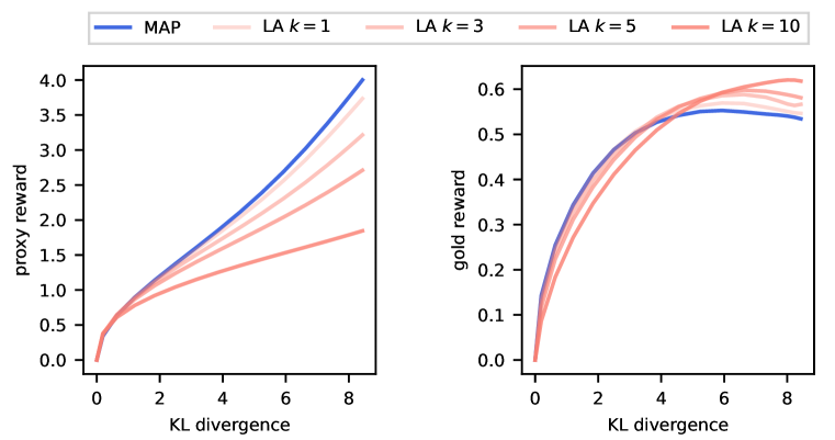
(a) Standard deviation-based penalty.

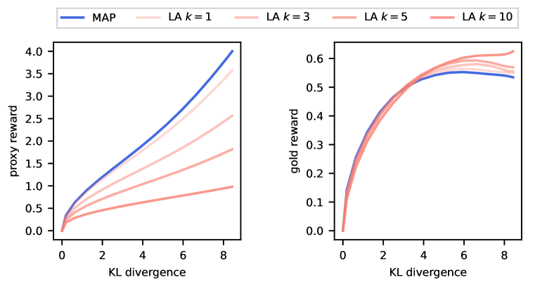
(b) Variance-based penalty.

Figure 1: Comparison of assigned rewards (normalized) between MAP and Laplace-LoRA reward models, across different uncertainty penalties and a range of $k$. Left column: compares the proxy reward model’s evaluation. Right column: compares the gold reward model’s evaluation.

We measured the policy performance under two reward models: the proxy reward model (Fig. 2(a) left and Fig. 2(b) left) and the gold-standard reward model (Fig. 2(a) right and Fig. 2(b) right), evaluated using the BoN estimator (Appendix A). As expected, there was always improvement as the number of samples increased when evaluated under the proxy reward model. However, looking at the gold reward model we observe reward overoptimization or hacking. In particular, the performance of the MAP reward, as evaluated under the gold reward model, actually starts to decrease for a very large KL divergence, and hence a very large number of BoN samples.

We found that taking uncertainty into account using Laplace-LoRA offered considerable benefits in these settings. The uncertainty penalty intensifies, particularly at higher levels of KL divergence, which is a promising indicator that Laplace-LoRA is effectively generating the anticipated uncertainty estimates, thereby enhancing the model’s ability to discern and appropriately penalize overconfident predictions in out-of-distribution scenarios. Fig. 2(a) shows a standard deviation based penalty (Eq. 15), while Fig. 2(b) shows a variance based penalty (Eq. 16). Overall the performance is similar, with perhaps a slight benefit for using variance-based methods, especially at a lower KL divergence.

6 Conclusion

We showed that using Laplace-LoRA to quantify uncertainty in reward models mitigates reward overoptimization in BoN sampling. Our findings highlight the potential of Bayesian approaches as valuable tools to provide uncertainty estimation in face of distribution shift, paving ways for more reliable and safer alignment of LLMs.

Appendix A Best-of-$n$ estimator

In this section, we review the BoN estimator for evaluating reward models (Nakano et al., 2021; Gao et al., 2023; Coste et al., 2024). Assume we have two reward models $r^{\text{train}}$ for ranking selecting responses and $r^{\text{val}}$ for evaluation, and queries are sampled from a query distribution $x\sim q(x)$ while responses are sampled from an LLM $y\sim p(y|x)$. For BoN sampling, we aim to sample $n$ responses $y_{1},...y_{n}$ from the LLM, and rank using $r_{\text{train}}$. We would like to compute the expected evaluation reward

$$\mathbb{E}_{x\sim q,y_{1},...,y_{n}\sim p}\Big{[}r^{\text{val}}\big{(}x,\operatorname*{argmax}_{y\in\{y_{1},...y_{n}\}}r^{\text{train}}(x,y)\big{)}\Big{]}.$$ (17)

The simplest approach is to use a Monte-Carlo estimator for the expectation. However, this requires repeated sampling of $n$ responses from the LLM which is costly. Instead, we consider sampling a fixed set of $N\geq n$ responses, and compute an unbiased estimator (for a single query $x$)

$$\frac{1}{\binom{N}{n}}\sum_{1\leq i_{1}\leq...\leq i_{n}\leq N}r^{\text{val}}\big{(}x,\operatorname*{argmax}_{y\in\{y_{i_{1}},...y_{i_{n}}\}}r^{\text{train}}(x,y)\big{)}.$$ (18)

If we sort the $N$ responses according to $r^{\text{train}}$ with $r^{\text{train}}(x,y_{1})\leq...\leq r^{\text{train}}(x,y_{N})$, the above estimator can be further simplified

$$\sum_{i=n}^{N}\frac{\binom{i-1}{n-1}}{\binom{N}{n}}r^{\text{val}}(x,y_{i})$$ (19)

by noting we only need to iterate the top response from $y_{n}$ to $y_{N}$, and select the rest $(n-1)$ responses from below. Finally, we take another Monte-Carlo sum over all queries $x_{1},...,x_{M}$.

Appendix B Experimental details

Here we present the experiment setups we used in our experiments. Table 1 shows the hyperparameters we used for fine-tuning the proxy reward model based on Pythia 70M.

Hyperparameter	Value
LoRA $r$	8
LoRA $\alpha$	16
Dropout Probability	0.1
Weight Decay	0
Learning Rate	$5\times 10^{-5}$
Learning Rate Scheduler	Linear
Batch Size	8
Max Sequence Length	300

Table 1: Hyperparameters used in fine-tuning Pythia 70M reward model with LoRA.

Appendix C Additional Experiments

In the main text, we have shown results for $k=1,3,5,10$. Here, we explore larger values $k=10,15,20,30$ as shown in Figure 2. We found larger penalties degrades performance of standard deviation-based penalty more significantly, while variance-based penalty is more robust.

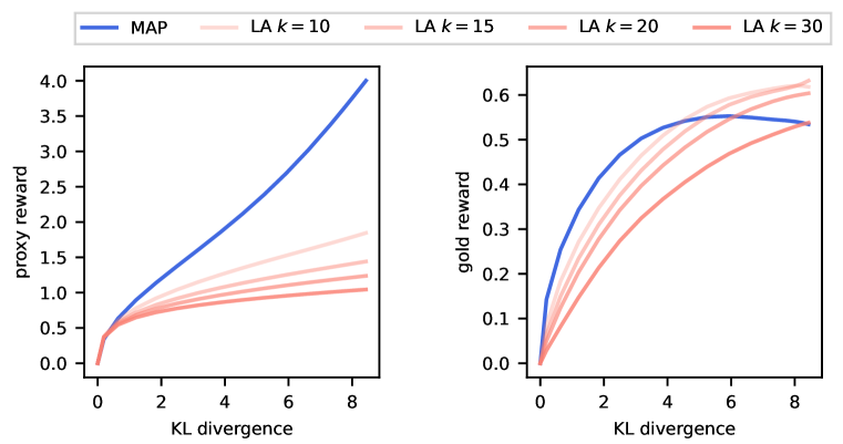
(a) Standard deviation-based penalty.

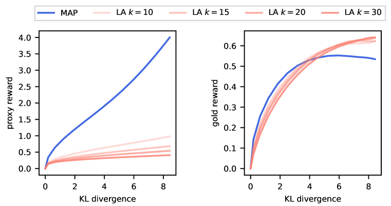
(b) Variance-based penalty.

Figure 2: Comparison of assigned rewards (normalized) between MAP and Laplace-LoRA reward models, across different uncertainty penalties and a range of $k$. Left column: compares the proxy reward model’s evaluation. Right column: compares the gold reward model’s evaluation.

References

- Aitchison et al. (2021) Laurence Aitchison, Adam Yang, and Sebastian W Ober. Deep kernel processes. In International Conference on Machine Learning, pp. 130–140. PMLR, 2021.
- Antorán et al. (2022) Javier Antorán, David Janz, James U Allingham, Erik Daxberger, Riccardo Rb Barbano, Eric Nalisnick, and José Miguel Hernández-Lobato. Adapting the linearised laplace model evidence for modern deep learning. In ICML, 2022.
- Bai et al. (2022) Yuntao Bai, Andy Jones, Kamal Ndousse, Amanda Askell, Anna Chen, Nova DasSarma, Dawn Drain, Stanislav Fort, Deep Ganguli, Tom Henighan, et al. Training a helpful and harmless assistant with reinforcement learning from human feedback. arXiv preprint arXiv:2204.05862, 2022.
- Biderman et al. (2023) Stella Biderman, Hailey Schoelkopf, Quentin Gregory Anthony, Herbie Bradley, Kyle O’Brien, Eric Hallahan, Mohammad Aflah Khan, Shivanshu Purohit, USVSN Sai Prashanth, Edward Raff, et al. Pythia: A suite for analyzing large language models across training and scaling. In International Conference on Machine Learning, pp. 2397–2430. PMLR, 2023.
- Blundell et al. (2015) Charles Blundell, Julien Cornebise, Koray Kavukcuoglu, and Daan Wierstra. Weight uncertainty in neural network. In International conference on machine learning, pp. 1613–1622. PMLR, 2015.
- Brantley et al. (2019) Kiante Brantley, Wen Sun, and Mikael Henaff. Disagreement-regularized imitation learning. In International Conference on Learning Representations, 2019.
- Chen et al. (2024) Lichang Chen, Chen Zhu, Davit Soselia, Jiuhai Chen, Tianyi Zhou, Tom Goldstein, Heng Huang, Mohammad Shoeybi, and Bryan Catanzaro. Odin: Disentangled reward mitigates hacking in rlhf. arXiv preprint arXiv:2402.07319, 2024.
- Coste et al. (2024) Thomas Coste, Usman Anwar, Robert Kirk, and David Krueger. Reward model ensembles help mitigate overoptimization. In ICLR, 2024.
- Daxberger et al. (2021) Erik Daxberger, Agustinus Kristiadi, Alexander Immer, Runa Eschenhagen, Matthias Bauer, and Philipp Hennig. Laplace redux-effortless bayesian deep learning. NeurIPS, 2021.
- Deng et al. (2022) Zhijie Deng, Feng Zhou, and Jun Zhu. Accelerated linearized laplace approximation for bayesian deep learning. NeurIPS, 2022.
- Dubois et al. (2024) Yann Dubois, Chen Xuechen Li, Rohan Taori, Tianyi Zhang, Ishaan Gulrajani, Jimmy Ba, Carlos Guestrin, Percy S Liang, and Tatsunori B Hashimoto. Alpacafarm: A simulation framework for methods that learn from human feedback. Advances in Neural Information Processing Systems, 36, 2024.
- Eisenstein et al. (2023) Jacob Eisenstein, Chirag Nagpal, Alekh Agarwal, Ahmad Beirami, Alex D’Amour, DJ Dvijotham, Adam Fisch, Katherine Heller, Stephen Pfohl, Deepak Ramachandran, et al. Helping or herding? reward model ensembles mitigate but do not eliminate reward hacking. arXiv preprint arXiv:2312.09244, 2023.
- Foong et al. (2019) Andrew YK Foong, Yingzhen Li, José Miguel Hernández-Lobato, and Richard E Turner. ’in-between’uncertainty in bayesian neural networks. In ICML Workshop on Uncertainty and Robustness in Deep Learning, 2019.
- Fortuin et al. (2021) Vincent Fortuin, Adrià Garriga-Alonso, Sebastian W Ober, Florian Wenzel, Gunnar Rätsch, Richard E Turner, Mark van der Wilk, and Laurence Aitchison. Bayesian neural network priors revisited. arXiv preprint arXiv:2102.06571, 2021.
- Gao et al. (2023) Leo Gao, John Schulman, and Jacob Hilton. Scaling laws for reward model overoptimization. In ICML, pp. 10835–10866, 2023.
- Gleave & Irving (2022) Adam Gleave and Geoffrey Irving. Uncertainty estimation for language reward models. arXiv preprint arXiv:2203.07472, 2022.
- Hu et al. (2021) Edward J Hu, Yelong Shen, Phillip Wallis, Zeyuan Allen-Zhu, Yuanzhi Li, Shean Wang, Lu Wang, and Weizhu Chen. Lora: Low-rank adaptation of large language models. arXiv preprint arXiv:2106.09685, 2021.
- Immer et al. (2021) Alexander Immer, Maciej Korzepa, and Matthias Bauer. Improving predictions of bayesian neural nets via local linearization. In AISTAT, 2021.
- Kristiadi et al. (2020) Agustinus Kristiadi, Matthias Hein, and Philipp Hennig. Being Bayesian, even just a bit, fixes overconfidence in relu networks. In ICML, 2020.
- Kristiadi et al. (2024) Agustinus Kristiadi, Felix Strieth-Kalthoff, Marta Skreta, Pascal Poupart, Alán Aspuru-Guzik, and Geoff Pleiss. A sober look at llms for material discovery: Are they actually good for bayesian optimization over molecules? arXiv preprint arXiv:2402.05015, 2024.
- Kunstner et al. (2019) Frederik Kunstner, Philipp Hennig, and Lukas Balles. Limitations of the empirical fisher approximation for natural gradient descent. Advances in neural information processing systems, 32, 2019.
- Lin et al. (2023) Yong Lin, Lu Tan, Hangyu Lin, Zeming Zheng, Renjie Pi, Jipeng Zhang, Shizhe Diao, Haoxiang Wang, Han Zhao, Yuan Yao, et al. Speciality vs generality: An empirical study on catastrophic forgetting in fine-tuning foundation models. arXiv preprint arXiv:2309.06256, 2023.
- MacKay (1992) David JC MacKay. A practical bayesian framework for backpropagation networks. Neural computation, 1992.
- Mangrulkar et al. (2022) Sourab Mangrulkar, Sylvain Gugger, Lysandre Debut, Younes Belkada, and Sayak Paul. Peft: State-of-the-art parameter-efficient fine-tuning methods. https://github.com/huggingface/peft, 2022.
- Nakano et al. (2021) Reiichiro Nakano, Jacob Hilton, Suchir Balaji, Jeff Wu, Long Ouyang, Christina Kim, Christopher Hesse, Shantanu Jain, Vineet Kosaraju, William Saunders, et al. Webgpt: Browser-assisted question-answering with human feedback. arXiv preprint arXiv:2112.09332, 2021.
- Ober & Aitchison (2021) Sebastian W Ober and Laurence Aitchison. Global inducing point variational posteriors for bayesian neural networks and deep gaussian processes. In International Conference on Machine Learning, pp. 8248–8259. PMLR, 2021.
- Ouyang et al. (2022) Long Ouyang, Jeffrey Wu, Xu Jiang, Diogo Almeida, Carroll Wainwright, Pamela Mishkin, Chong Zhang, Sandhini Agarwal, Katarina Slama, Alex Ray, et al. Training language models to follow instructions with human feedback. Advances in Neural Information Processing Systems, 35:27730–27744, 2022.
- Ramé et al. (2024) Alexandre Ramé, Nino Vieillard, Léonard Hussenot, Robert Dadashi, Geoffrey Cideron, Olivier Bachem, and Johan Ferret. Warm: On the benefits of weight averaged reward models. arXiv preprint arXiv:2401.12187, 2024.
- Shi & Lipani (2023) Zhengxiang Shi and Aldo Lipani. Dept: Decomposed prompt tuning for parameter-efficient fine-tuning. arXiv preprint arXiv:2309.05173, 2023.
- Stiennon et al. (2020) Nisan Stiennon, Long Ouyang, Jeffrey Wu, Daniel Ziegler, Ryan Lowe, Chelsea Voss, Alec Radford, Dario Amodei, and Paul F Christiano. Learning to summarize with human feedback. Advances in Neural Information Processing Systems, 33:3008–3021, 2020.
- Touvron et al. (2023) Hugo Touvron, Thibaut Lavril, Gautier Izacard, Xavier Martinet, Marie-Anne Lachaux, Timothée Lacroix, Baptiste Rozière, Naman Goyal, Eric Hambro, Faisal Azhar, et al. Llama: Open and efficient foundation language models. arXiv preprint arXiv:2302.13971, 2023.
- Wang et al. (2023) Xi Wang, Laurence Aitchison, and Maja Rudolph. Lora ensembles for large language model fine-tuning. arXiv preprint arXiv:2310.00035, 2023.
- Yang et al. (2024) Adam X Yang, Maxime Robeyns, Xi Wang, and Laurence Aitchison. Bayesian low-rank adaptation for large language models. In ICLR, 2024.
- Zhai et al. (2024) Yuanzhao Zhai, Han Zhang, Yu Lei, Yue Yu, Kele Xu, Dawei Feng, Bo Ding, and Huaimin Wang. Uncertainty-penalized reinforcement learning from human feedback with diverse reward lora ensembles. arXiv preprint arXiv:2401.00243, 2024.
- Zhang et al. (2019) Ruqi Zhang, Chunyuan Li, Jianyi Zhang, Changyou Chen, and Andrew Gordon Wilson. Cyclical stochastic gradient mcmc for bayesian deep learning. arXiv preprint arXiv:1902.03932, 2019.
- Zhang et al. (2024) Shun Zhang, Zhenfang Chen, Sunli Chen, Yikang Shen, Zhiqing Sun, and Chuang Gan. Improving reinforcement learning from human feedback with efficient reward model ensemble. arXiv preprint arXiv:2401.16635, 2024.