Spatial Queues with Nearest Neighbour Shifts

Abstract

In this work we study multi-server queues on a Euclidean space. Consider $N$ servers that are distributed uniformly in $[0,1]^{d}$. Customers (users) arrive at the servers according to independent Poisson processes of intensity $\lambda$. However, they probabilistically decide whether to join the queue they arrived at, or move to one of the nearest neighbours. The strategy followed by the customers affects the load on the servers in the long run. In this paper, we are interested in characterizing the fraction of servers that bear a larger load as compared to when the users do not follow any strategy, i.e., they join the queue they arrive at. These are called overloaded servers. In the one-dimensional case ($d=1$), we evaluate the expected fraction of overloaded servers for any finite $N$ when the users follow probabilistic nearest neighbour shift strategies. Additionally, for servers distributed in a $d$-dimensional space we provide expressions for the fraction of overloaded servers in the system as the total number of servers $N\rightarrow\infty$. Numerical experiments are provided to support our claims. Typical applications of our results include electric vehicles queueing at charging stations, and queues in airports or supermarkets.

1 Introduction

Traditional queueing systems involve multiple queues interacting with each other. The analysis of the queueing mechanism and related load balancing questions are tractable owing to the product-form stationary distribution. Most earlier works on queues distributed spatially involve customers arriving at random locations in a Euclidean space and a server travelling to serve them. However, most queueing networks in the present day involve servers that are distributed in space and arrivals deciding among multiple servers. This work addresses the problem of load distribution in such networks where the servers are spatially distributed and the arrivals decide to join a server based on proximity.

As a motivating example, consider the rapidly growing electric vehicles (EV) industry. With increased adaptation of EVs, the charging infrastructure is also being scaled up. However, physical and financial constraints put a cap on the number of charging stations that can be deployed. In such a scenario, it is natural to expect EV users to adopt strategies in order to minimize their waiting times at charging stations. For example, a user on arriving at a charging station and finding it to be occupied, might decide to travel to a farther station in the hope that it would be empty. The user strategy affects the load that is perceived at the servers in the long run. Some of the servers get overloaded which might degrade the performance of the system on the whole. An understanding of the fraction of overloaded servers helps in optimal resource allocation preventing such degradation. Additionally, monitoring the fraction of overloaded servers can be used to incentivize customers to change their strategies thus increasing the durability of the entire system. Similar considerations arise in other practical networks involving queues, like supermarkets, airports etc.

Motivated by such applications, in this work we consider a set of $N$ servers that are deployed in a Euclidean space with queues at each of them modelled as Poisson arrival processes. In the context of EVs, the servers are the charging stations, and a Poisson arrival process models the EV users arriving at a charging station. EV charging stations have been modelled as a Poisson point process in two dimensional space in several previous works (see, for e.g., [7, 15, 2]). However, the problem that authors address in these works pertain to optimal placement of charging stations in the underlying space.

Another line of work that considers queues on spaces are polling systems. One of the earlier works in this domain [1] considers multiple queues in a convex space with a single server moving across to serve them. Several later works, such as [10, 19], study vehicle routes and delay in such systems. In all of these (and some related) works there is a single server and there is no interaction between different queues.

In contrast, in the present work we consider queues where customers from one queue probabilistically move to a queue which is located close to it in the underlying space. Customers changing queues has been referred to as jockeying in the queueing theory terminology. There has been considerable work on jockeying in queues in the past [11, 8, 13]. The focus in these works is predominantly to analyse the steady-state distribution or find expected line-lengths or delays. However, they primarily consider two server systems with no spatial component in the problem.

The closest work to ours is [18] where the authors consider arrivals occurring on the two-dimensional torus, with multiple servers following a greedy strategy to serve the customers by travelling minimally. They find that such a strategy results in servers coalescing making the system inefficient. In contrast, in our work the servers are fixed whereas the arrivals follow nearest neighbour strategies and hence the two works are not directly comparable.

More precisely, in the current work, $N$ servers are deployed in a Euclidean space and customers arriving into a queue decide whether to stay or to move to a queue nearest to them with a prescribed probability. We call such strategies as nearest neighbour shift (NNS) strategies. The metric of interest is the expected fraction of overloaded servers in the system which we characterize for users following an NNS strategy.

We begin by describing our system model and state the main results in Section 2. This is followed by the analysis of NNS strategies for one dimension in Section 3 and for higher dimensions in Section 4. Section 5 provides numerical simulations justifying our results and Section 6 highlights some future directions.

2 System model and main results

Consider $N$ servers distributed uniformly within a finite area $\Gamma=\left[0,1\right]^{d}$, $d\geq 1$, equipped with the standard Euclidean metric. Let $\{X_{i}\}_{i=1}^{N}$ denote the locations of the servers. Each server has a service rate of $\mu$. A server $i$ is associated with a Poisson arrival process of intensity $\lambda<\mu$ denoted using $N_{i}(t)$ as a function of time $t$.

Customers on arriving at a queue can adopt different strategies. In this work, we consider all customers to be identical who make independent decisions. Our interest is in nearest neighbour shift (NNS) strategies which we describe next.

• $(k,p)$-NNS strategy: Customers join the queue they arrive at with probability $p\in[0,1]$, or join the queue at one of the $k\geq 1$ nearest servers chosen uniformly at random with the remaining probability. More precisely, define $\mathcal{N}_{k}(u)$ to be the $k$ nearest servers to $u\in[N]$. Then, a customer arriving at server $u$ joins the queue at $u$ with probability $p$ or joins the queue at $v\in\mathcal{N}_{k}(u)$ with probability $\frac{1-p}{k}$.

Naturally, ’near’ness between servers is measured with respect to the Euclidean metric attributed to the space $\Gamma$. The servers within $\mathcal{N}_{k}(\cdot)$ are also referred to as the $k$-nearest neighbours from which the strategy derives its name. Additionally, for a server $u$, the term the nearest neighbour of $u$ refers to its $1$-nearest neighbour. In the course of our analysis, we will require the following variants of the $(k,p)$-NNS strategy for which we attribute their own names.

• $k\geq 1,p=1$: null strategy
  Customers arriving to a queue stay in (join) the same queue.

• $k=1,p=0$: only nearest neighbour shift strategy (oNNS)
  Customers arriving to a queue join the nearest neighbour.

• $k\geq 1,p=0$: pure $k$ nearest neighbour shift strategy (pure $k$-NNS)
  Customers arriving to a queue join one of the $k$-nearest neighbours with equal probability.

In all the strategies, note the distinction that is made between a customer arriving at a queue and joining a queue.

Our goal is to characterize the expected fraction of overloaded servers in the system. To go about this, we first define the load at a particular server as the asymptotic rate of the number of customers served in that queue. To be more precise, let $J_{i}(t)$ be the number of customers who join the queue at server $i$ till time $t$. The asymptotic load (or just, load) at server $i$ is defined as

$$L_{i}:=\lim_{t\rightarrow\infty}\frac{J_{i}(t)}{t}.$$ (1)

We refer to this as the load since servers with a large value of $L_{i}$ have more arrivals in the long term as compared to servers with a small $L_{i}$ value, which degrades their performance.

Under the null strategy, the asymptotic load at a server is almost surely (a.s.) $L_{i}=\lambda$ for all $1\leq i\leq N$. However, when the customers follow other strategies on arriving at a queue, the load on each server changes. Some servers will have a load larger than $\lambda$ and some smaller. Our interest is in the fraction of overloaded servers which is defined as

$$\mathcal{O}_{N}:=\frac{\left|\left\{i:\lim_{t\rightarrow\infty}\frac{J_{i}(t)}{t}>\lambda\quad\text{a.s.}\right\}\right|}{N},$$ (2)

where $|\cdot|$ denotes the cardinality.

We next analyze the $(k,p)$-NNS strategy and characterize the expected fraction of overloaded servers for any $N$ in one dimension ($d=1$). Specifically, for the $(1,p)$-NNS strategy, we find that a quarter of the servers get overloaded in the long run irrespective of the value of $p$ in one dimension which is stated in the following theorem.

Theorem 2.1.

For $N$ servers distributed uniformly in $[0,1]$ with Poisson arrivals of intensity $\lambda$ following the $(1,p)$-NNS strategy with, the asymptotic load at any node $i\in[N]$ satisfies

$$L_{i}\in\{p\lambda,\lambda,(2-p)\lambda\}\qquad\qquad\text{a.s.,}$$

and the expected fraction of overloaded servers is $\mathbb{E}\mathcal{O}_{N}=\frac{1}{4}.$

In the process of proving this theorem, we also obtain the expected fraction of servers with all possible loads which is shown in Section 3. For higher dimensions, we obtain convergence results for the fraction of overloaded servers as $N\rightarrow\infty$. This is stated in the following theorem.

Theorem 2.2.

Consider $N$ servers distributed uniformly in $[0,1]^{d}$ with Poisson arrivals of intensity $\lambda$ following the $(k,p)$-NNS strategy. For any $v\in[N]$, the asymptotic load satisfies

$$L_{v}\in\Bigg{\{}\lambda\left[\frac{j}{k}+\left(1-\frac{j}{k}\right)p\right],j\in\{0,1,\cdots,\kappa k\}\Bigg{\}}\qquad\text{a.s.,}$$

and the fraction of overloaded servers satisfies

$$\mathcal{O}_{N}\rightarrow\sum_{j=k+1}^{\kappa k}q_{j}(d,k)\hskip 14.22636pt\text{a.s.}\hskip 14.22636pt\text{ as }N\rightarrow\infty.$$

The constants $\kappa$ and $q_{j}(d,k)$ are explained in Section 4. Before we proceed, we remark here on the boundary conditions for the underlying space $[0,1]^{d}$. Since servers are uniformly distributed, the fraction of servers that fall near the boundary diminishes as $N$ increases. Thus, neglecting the servers on the boundary does not affect the fraction of overloaded servers in (2) for large $N$. Alternately, this also means that we are allowed to take any boundary conditions that renders the analysis easy. In the case of dimension $d=1$, we take fixed boundary conditions where the servers closest to $0$ and $1$ constitute the boundary servers. Taking toroidal boundary conditions by gluing the ends $0$ and $1$ together does not alter our results. However, some of the arguments in our proofs have to be made differently.

3 One dimension $d=1$, and $k=1$

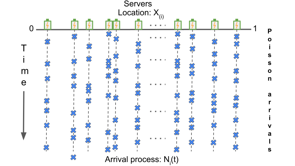
Figure 1: EVs arriving as a Poisson process into charging stations distributed uniformly on $[0,1]$.

The case of dimension $d=1$ is interesting in its own right since it can be motivated by numerous applications. With reference to the examples discussed in the introduction, EV charging stations located on a highway and checkout counters at supermarkets correspond to queues on a $1$D space. An illustration for a $1$D system is provided in Fig. 1.

In this section, we first provide some preliminaries in Section 3.1 required for the case of $d=1$. We define and analyze a deterministic strategy called oNNS in Section 3.2 that will aid us in the analysis of the probabilistic NNS strategies which is done in Section 3.3.

3.1 Preliminaries

The primary tool that we will use in the $1$D case are the order statistics of the server locations which we define below. Let $X_{1},\cdots,X_{N}$ be iid random variables from a distribution $F(\cdot)$ with density $f(\cdot)$ supported on $[0,1]$. When arranged in the order of magnitude and then written as $X_{(1)}\leq X_{(2)}\leq\cdots\leq X_{(N)}$, the random variable $X_{(i)}$ is called the $i$-th order statistic, and together they are referred to as the order statistics of $X_{1},\cdots,X_{N}$.

The following are some facts about order statistics that will be used in our analysis (see e.g., [6, 17]). These are stated for $f(x)=\mathbf{1}\{x\in[0,1]\}$ and $F(x)=\int_{0}^{x}f(x)dx$ since in our case the servers are distributed uniformly in $[0,1]$.

• Fact 1: Conditioned on $X_{(i)}=a$, the random variables $X_{(1)},\cdots,X_{(i-1)}$ are the order statistics of

  $$Y_{1},\cdots,Y_{i-1}\stackrel{{\scriptstyle\text{iid}}}{{\sim}}\text{ Unif }\left([0,a]\right),$$ (3)

  and $X_{(i+1)},\cdots,X_{(N)}$ are the order statistics of

  $$Y_{i+1},\cdots,Y_{N}\stackrel{{\scriptstyle\text{iid}}}{{\sim}}\text{ Unif }\left([a,1]\right),$$ (4)

  and, moreover $X_{(1)},\cdots,X_{(i-1)}$ are (conditionally) independent of $X_{(i+1)},\cdots,X_{(N)}$.

• Fact 2: The joint density of the $i$-th and the $j$-th order statistic for $i<j$ is given by

  $$f_{i,j}(r,s) =\frac{N!}{(i-1)!(j-i-1)!(N-j)!}F(r)^{i-1}f(r)$$

  $$\ \hskip 56.9055pt\times\left[F(s)-F(r)\right]^{j-i-1}f(s)[1-F(s)]^{N-j}.$$ (5)

3.2 oNNS strategy

Before investigating the $(k,p)$-NNS strategy which is probabilistic in nature, we look into the deterministic oNNS strategy. This will help us to address the probabilistic strategies.

In the oNNS strategy, customers on arriving at queue $i$ join the queue at the nearest neighbour of $i$. The arrivals to servers on the boundary ($X_{(1)}$ and $X_{(N)}$) join the adjacent queues ($X_{(2)}$ and $X_{(N-1)}$ respectively). The following lemma provides the possible loads at the servers when arrivals follow the oNNS strategy.

Lemma 3.1.

Consider $N$ servers distributed uniformly in $[0,1]$ with Poisson arrivals of intensity $\lambda$ following the oNNS strategy. For any $i\in[N]$, the asymptotic load satisfies

$$L_{i}\in\{0,\lambda,2\lambda\}\hskip 28.45274pt\text{ a.s..}$$

Proof.

Arrivals to the left and right neighbours of server $i$ could both join the queue at $i$ resulting in $L_{i}=2\lambda\ \text{a.s.}$. If only arrivals to one of the neighbours of $i$ join the queue at $i$, $L_{i}=\lambda\ \text{a.s.}$ and if neither join the queue at $i$, it results in $L_{i}=0\ \text{a.s.}$. ∎

Owing to Lemma 3.1, we define the fraction of servers with load $s\lambda$ as

$$R_{s}:=\frac{\left|\left\{i:\lim_{t\rightarrow\infty}\frac{J_{i}(t)}{t}=s\lambda\quad\text{a.s.}\right\}\right|}{N},$$

for $s=0,1,2$. Since there are $N$ queues with equal arrival rates of $\lambda$, we have that $R_{0}+R_{1}+R_{2}=1$. The expected fraction of servers with loads of $0,\lambda,2\lambda$ is characterized in the following lemma.

Lemma 3.2.

For $N$ servers distributed uniformly in $[0,1]$ with Poisson arrivals of intensity $\lambda$ following the oNNS strategy,

$$\mathbb{E}R_{0}=\frac{1}{4},\ \ \ \mathbb{E}R_{1}=\frac{1}{2},\ \ \text{ and }\mathbb{E}R_{2}=\frac{1}{4}.$$

Proof.

Let $X_{(1)},\cdots,X_{(N)}$ denote the order statistics of the locations of the $N$ servers. In the following discussion, node $i$ will refer to the $i$-th order statistic. The asymptotic load at node $i$ is $0$ if the arrivals to both the $(i-1)$-th and the $(i+1)$-th node do not join the $i$-th node. This happens if and only if both the events $E_{i}^{+}:=\{X_{(i+2)}-X_{(i+1)}<X_{(i+1)}-X_{(i)}\}$ and $E_{i}^{-}:=\{X_{(i-1)}-X_{(i-2)}<X_{(i)}-X_{(i-1)}\}$ occur simultaneously. We first compute the probability of the event $E_{i}^{+}\cap E_{i}^{-}$.

From Fact 1 of Section 3.1, conditioned on the value of $X_{(i)}=x$, the events $E_{i}^{+}$ and $E_{i}^{-}$ are independent. Thus

$$\mathbb{P}(E_{i}^{+}\cap E_{i}^{-}) =\int_{0}^{1}\mathbb{P}(X_{(i+2)}>2X_{(i+1)}-x|X_{(i)}=x)$$

$$\qquad\qquad\mathbb{P}(X_{(i-2)}>2X_{(i-1)}-x|X_{(i)}=x)f_{X_{(i)}}(x)dx,$$ (6)

where $f_{X_{(i)}}(\cdot)$ is the density of the $i$-th order statistic. We will now evaluate each of the probabilities in the above expression using (3), (4) and (5). For this, we first write down the joint distribution of the $j$-th and the $(j+1)$-th order statistic using (5) to be

$$f_{j,j+1}(r,s)=N!\ \frac{F(r)^{j-1}f(r)f(s)(1-F(s))^{N-j-1}}{(j-1)!(N-j-1)!}.$$ (7)

Using (3), (4) with (7) the required integral can be computed as follows: (see Fig. 2)

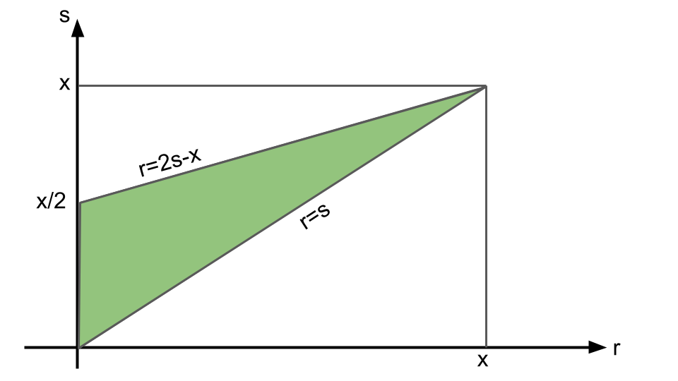
Figure 2: Region of integration.

$$\mathbb{P}(X_{(i-2)} >2X_{(i-1)}-x|X_{(i)}=x)$$

$$=\int_{0}^{x}\int_{0}^{s}\frac{(i-1)!}{(i-3)!}\left(\frac{r^{i-3}}{x^{i-1}}\right)\ drds-\int_{\frac{x}{2}}^{x}\int_{0}^{2s-x}\frac{(i-1)!}{(i-3)!}\left(\frac{r^{i-3}}{x^{i-1}}\right)\ drds$$

$$=\int_{0}^{x}\frac{(i-1)(i-2)}{x^{i-1}}\left(\frac{s^{i-2}}{i-2}\right)ds-\int_{\frac{x}{2}}^{x}\frac{(i-1)(i-2)}{x^{i-1}}\left(\frac{(2s-x)^{i-2}}{i-2}\right)ds$$

$$=\frac{i-1}{x^{i-1}}\int_{0}^{x}s^{i-2}\ ds-\frac{i-1}{x^{i-1}}\int_{\frac{x}{2}}^{x}(2s-x)^{i-2}\ ds$$

$$=1-\frac{i-1}{x^{i-1}}\int_{\frac{x}{2}}^{x}(2s-x)^{i-2}\ ds=\frac{1}{2}.$$

and similarly $\mathbb{P}(X_{(i+2)}>2X_{(i+1)}-x|X_{(i)}=x)=\frac{1}{2}.$ Substituting this in (6), we obtain

$$\mathbb{P}(E_{i}^{+}\cap E_{i}^{-})=\int_{0}^{1}\frac{f_{X_{(i)}}(x)}{4}dx=\frac{1}{4}.$$

Since $\mathbb{E}R_{0}=\frac{1}{N}\mathbb{E}\left[\sum_{i=1}^{N}\mathbf{1}\{E_{i}^{+}\cap E_{i}^{-}\}\right]$, we have that $\mathbb{E}R_{0}=\frac{1}{4}$. Similar computations for $\mathbb{E}R_{1}$ and $\mathbb{E}R_{2}$ can be shown which proves the theorem. ∎

An intuitive interpretation for the result in Lemma 3.2 stems from the distribution of consecutive order statistics, also referred to as uniform spacings. Define the inter-node distances $Y_{j}=X_{(j)}-X_{(j-1)}$ for $j\in\{i-1,i,i+1,i+2\}$ (see Fig. 3). The asymptotic load at node $i$ as a function of these distances is shown in Table 1. Since the nodes are uniformly distributed, each row of Table 1 has equal probability of $\frac{1}{4}$ each. Using these probabilities to compute the expected value of $R_{s}$ (as in the proof of Lemma 3.2), we have the desired result.

$Y_{i}\ ?\ Y_{i-1}$	$Y_{i+2}\ ?\ Y_{i+1}$	$\displaystyle{\lim_{t\rightarrow\infty}\frac{Q_{i}(t)}{t}}$
$<$	$<$	$1$
$<$	$>$	$2$
$>$	$<$	$0$
$>$	$>$	$1$

Table 1: Asymptotic load of a node as a function of inter-node distances. (Replace ? by the inequality.)

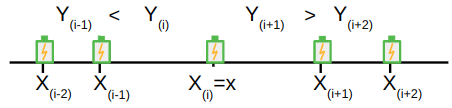
Figure 3: Illustration for the load at node $X_{(i)}$ being $0$.

In fact, a stronger statement to Lemma 3.2 holds for $R_{0}$ and $R_{2}$ which is stated below.

Proposition 3.3.

For $N$ servers distributed uniformly in $[0,1]$ with Poisson arrivals of intensity $\lambda$ following the oNNS strategy,

$$R_{0}=R_{2}\qquad\ \ \text{a.s.}$$

Proof.

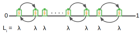
(a) Case 1: $R_{0}=0$

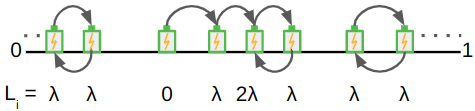
(b) Case 2: $R_{0}>0$

Figure 4: Illustration for $R_{0}=R_{2}$ a.s.. An arrow from server $i$ to server $j$ indicates that customers arriving at server $i$ join the queue at $j$.

The arguments in this proof are made for each realization in the underlying probability space. Recall that $L_{i}$ was defined to be the asymptotic load at server $i$, i.e., $L_{i}=\lim_{t\rightarrow\infty}\frac{J_{i}(t)}{t}\in\{0,\lambda,2\lambda\}$. Note that $\sum_{i}\frac{L_{i}}{N\lambda}=1=R_{0}+R_{1}+R_{2}$. Define $S_{i}:=\frac{L_{i}}{\lambda}$ so that $\sum_{i=1}^{N}S_{i}=N$. The proof is divided into two cases. See Fig. 4 for an illustration of the two cases.
Case 1: $R_{0}=0$
Owing to the fixed boundary conditions, the closest neighbour to the queue at $X_{(1)}$ is the queue at $X_{(2)}$. The only possible way that $R_{0}=0$ is if arrivals to $X_{(2)}$ join the queue at $X_{(1)}$. Now suppose that the arrivals to the queue at $X_{(3)}$ join $X_{(2)}$, then $\sum_{i=3}^{N}S_{i}=N-3$ since $S_{1}=1$ and $S_{2}=2$. For this to hold at least one of the summands, $S_{i}$, needs to be equal to zero. However, this is not possible since $R_{0}=0$. Therefore, arrivals to $X_{(3)}$ cannot join $X_{(2)}$ but must join $X_{(4)}$ resulting in $S_{1}=S_{2}=1$. The nodes from $X_{(3)}$ to $X_{(N)}$ now form a system of $N-2$ nodes with the property that $R_{0}=0$. Recursing over the same argument, we obtain $S_{i}=1$ for all $i\in[N]$. Equivalently $R_{0}=R_{2}=0$.
Case 2: $R_{0}>0$
Let node $i$ be such that $S_{i}=0$. Suppose that the arrival to node $i$ joins $X_{(i+1)}$ (a similar argument goes through if it joins $X_{(i-1)}$ instead). Since $S_{i}=0$, arrivals to $X_{(i+1)}$ should join $X_{(i+2)}$. For $j\geq 2$, arrivals to $X_{(i+j)}$ can join either $X_{(i+j-1)}$ or $X_{(i+j+1)}$. If for some $j$, arrivals to $X_{(i+j)}$ join $X_{(i+j-1)}$ then $S_{(i+j-1)}=2$. Note that there must always exist such a node $j$ owing to our boundary conditions that arrivals to nodes $0$ and $N$ join nodes $1$ and $N-1$ respectively. Thus $S_{i}=0$, $S_{i+1}=1,\cdots,S_{i+j-2}=1$ and $S_{i+j-1}=2$. Removing the nodes $k\in\{i,\cdots,i+j-1\}$ results in $N-j$ nodes with $NR_{0}-1$ number of nodes with $0$ asymptotic load. Repeating the same procedure by choosing a node $i^{\prime}$ with $S_{i^{\prime}}=0$ iteratively decrements the value of $NR_{0}$ in each iteration, finally resulting in $NR_{0}=0$. The remaining nodes have an asymptotic load of $\lambda$ each. Note that each removal step comprises of a node with $S_{i}=0$ and a node with $S_{i+j-1}=2$. This shows that $R_{0}=R_{2}$ pointwise from which the statement of the lemma follows. ∎

Returning to the problem of characterizing the quantity $\mathcal{O}_{N}$, since the overloaded servers are precisely those with a load greater than $\lambda$, in the one dimensional case we have that $\mathcal{O}_{N}=R_{2}$. Thus, we obtain the following lemma as a direct consequence of Lemma 3.2.

Lemma 3.4.

For $N$ servers distributed uniformly in $[0,1]$ with Poisson arrivals of intensity $\lambda$ following the oNNS strategy, the expected fraction of overloaded servers is $\mathbb{E}\mathcal{O}_{N}=\frac{1}{4}$.

We are now in a position to tackle the probabilistic NNS strategies.

3.3 $(1,p)$-NNS strategy

We first establish additional terminologies to convey the ideas clearly. Designate a customer as lazy if on arrival at a queue, the user joins it, or as active if the user joins the queue at the nearest neighbour. Denote the fraction of servers with an asymptotic load of $s\lambda$ by

$$R_{s}:=\frac{\left|\left\{i:\lim_{t\rightarrow\infty}\frac{J_{i}(t)}{t}=s\lambda\quad\text{a.s.}\right\}\right|}{N}.$$

The following theorem characterizes the expected value of $R_{s}$ for all possible asymptotic loads $s\lambda$ in the $(1,p)$-NNS strategy.

Theorem 3.5.

For $N$ servers distributed uniformly in $[0,1]$ with Poisson arrivals of intensity $\lambda$ following the $(1,p)$-NNS strategy with (lazy) probability $p\in[0,1]$, the asymptotic load at any node $i\in[N]$ satisfies

$$L_{i}\in\{p\lambda,\lambda,(2-p)\lambda\}\qquad\qquad\text{a.s.,}$$

and the expected fraction of servers with these loads are

$$\mathbb{E}R_{p}=\frac{1}{4},\ \ \ \mathbb{E}R_{1}=\frac{1}{2},\ \ \text{ and }\ \ \mathbb{E}R_{2-p}=\frac{1}{4}.$$

Consequently, $\mathbb{E}\mathcal{O}_{N}=\mathbb{E}R_{2-p}=\frac{1}{4}$.

Proof.

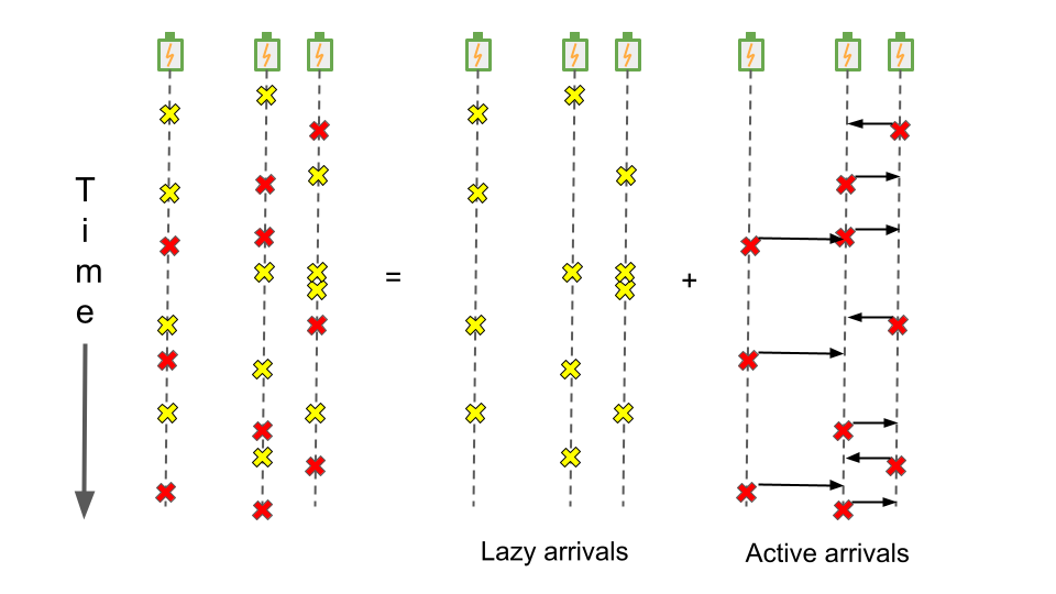
Figure 5: Arrival process decomposition into lazy and active users. The arrows indicate the shifts to the nearest neighbours for active users.

First, we find the asymptotic loads that are possible for each server. Owing to the thinning property of the Poisson process, the arrivals to queue $i$ can be decomposed into two independent Poisson processes: the lazy process $N_{i}^{L}(t)$ of intensity $\lambda p$ and the active process $N_{i}^{A}(t)$ of intensity $\lambda(1-p)$ as shown in Fig. 5. Accordingly, the contribution towards the load at server $i$ comprises of the lazy component $J_{i}^{L}(t)$ from arrivals $N_{i}^{L}(t)$, and the active component $J_{i}^{A}(t)$ from nearest neighbours of $i$ whose arrivals join the queue at $i$. The asymptotic load at any node $i$ is given by $\lim_{t\rightarrow\infty}\frac{J_{i}(t)}{t}=\lim_{t\rightarrow\infty}\frac{J_{i}^{L}(t)}{t}+\lim_{t\rightarrow\infty}\frac{J_{i}^{A}(t)}{t}$. For the lazy component $\lim_{t\rightarrow\infty}\frac{J_{i}^{L}(t)}{t}=p\lambda$ a.s., since arrivals of $N_{i}^{L}(t)$ contribute to $J_{i}^{L}(t)$. For the active component, arrivals in $N_{i}^{A}(t)$ behave as in the oNNS strategy. Since $N_{i}^{A}(t)$ is a Poisson arrival process of intensity $\lambda(1-p)$, we obtain,

$$\lim_{t\rightarrow\infty}\frac{J_{i}^{A}(t)}{t}\in\{0,\lambda(1-p),2\lambda(1-p)\}\qquad\qquad\text{a.s..}$$

Hence the possible asymptotic loads are

$$\lim_{t\rightarrow\infty}\frac{J_{i}(t)}{t}\in\{p\lambda,\lambda,(2-p)\lambda\}\qquad\qquad\text{a.s..}$$

Next, we find the expected fraction of servers with each of the individual asymptotic loads computed above. To illustrate, consider

$$\mathbb{E}R_{p} =\frac{1}{N}\mathbb{E}\left[\sum_{i=1}^{N}\mathbf{1}\left\{\lim_{t\rightarrow\infty}\frac{J_{i}(t)}{t}=p\lambda\right\}\right]$$

$$=\frac{1}{N}\sum_{i=1}^{N}\mathbb{P}\left(\lim_{t\rightarrow\infty}\frac{J^{L}_{i}(t)}{t}=p\lambda\ \text{ and }\ \lim_{t\rightarrow\infty}\frac{J^{A}_{i}(t)}{t}=0\right)$$

The two events are independent since they are functions of independent Poisson processes $N_{i}^{L}(t)$ and $N_{i}^{A}(t)$. The term $\mathbb{P}\left(\lim_{t\rightarrow\infty}\frac{J^{L}_{i}(t)}{t}=p\lambda\right)$ corresponds to the null strategy in the lazy component and is equal to $1$. The term $\mathbb{P}\left(\lim_{t\rightarrow\infty}\frac{J^{A}_{i}(t)}{t}=0\right)$ can be obtained via the oNNS strategy for the active component. Using Lemma 3.2 for the active component $N_{i}^{A}(t)$ yields $\mathbb{E}R_{p}=\frac{1}{4}$.

Similar derivations follow for the expected fraction of servers with other asymptotic loads giving $\mathbb{E}R_{1}=\frac{1}{2},\text{ and }\mathbb{E}R_{2-p}=\frac{1}{4}$. ∎

Notice that when $p=0$ we obtain Lemma 3.2 for the oNNS strategy and for $p=1$, we obtain $\mathbb{E}R_{1}=1$ corresponding to the null strategy.

In one dimension, the $(k,p)$-NNS strategies for $k>2$ are not practically relevant for the application of electric vehicles. This is because customers when restricted to a line choose one of the directions –left (with prob. $\ell$) or right (with prob. $r$)– and proceed to the nearest server in that direction (or stay in the same queue with prob. $1-r-\ell$). For such a left-right nearest neighbour shift ($\ell r$-NNS) strategy, the following theorem asserts that there are no overloaded servers.

Theorem 3.6.

For $N$ servers distributed uniformly in $[0,1]$ with Poisson arrivals of intensity $\lambda$ following the $\ell r$-NNS strategy with parameters $r$ and $\ell$ we have $\mathbb{E}R_{1}=1.$

Proof.

The proof follows on the same lines as the proof of Theorem 3.5 by decomposing the arrivals at a particular queue into independent thinned point processes of intensity $r$, $\ell$ and $1-r-\ell$. The asymptotic load at a server is the net load due to each of these arrivals and is equal to $L_{i}=(r+\ell+1-r-\ell)\lambda=\lambda$. Since this is the load at every server (even the boundary), the theorem is proved. ∎

Nevertheless, we address the case of general $k$ for general dimensions $d$ in the next section and comment on the implications of our results for queues in one dimension.

4 General dimension $d\geq 1$ and general $k\geq 1$

The analysis in the previous section does not easily carry over to higher dimensions since order statistics are particular to the one dimensional case. In this section, we investigate the problem on a general dimension $d\geq 1$ where the arrivals follow $(k,p)$-NNS strategies with any $k\geq 1$.

4.1 Preliminaries

The routing graph $G^{N}_{k}=(V,E)$ is a directed graph on the vertex set $V=\{X_{1},\cdots,X_{N}\}$ where the vertices are distributed uniformly in $[0,1]^{d}$, and the edge set is constructed in the following way: add a directed edge $u\longrightarrow v$, if node $v$ is one of the $k$-nearest neighbours of node $u$. This has been referred to as the NN graph or the NN digraph in previous literature (see e.g., [9]). The in-degree of a vertex $u$ is the number of incoming edges to $u$, i.e., $|\{v:v\longrightarrow u\}|$ and the out-degree is the number of outgoing edges from $u$ i.e., $|\{v:u\longrightarrow v\}|$. Some properties of the routing graph are listed below:

1. Every node $u\in G^{N}_{k}$ has out-degree $k$.

2. There exists a constant $\kappa\equiv\kappa(d)$ such that the maximum in-degree of a node in $G_{k}^{N}$ is at most $\kappa k$ almost surely. The constant $\kappa(d)$ is defined as the maximum number of points $a_{1},a_{2},\cdots,a_{m}$ on the unit sphere in $\mathbb{R}^{d}$ such that for all $1\leq i\neq j\leq m$, $\|a_{i}-a_{j}\|>1$. In particular, it is known that $\kappa(1)=2$ and $\kappa(2)=5$.

A directed graph $H_{k}^{1}=(V_{k}^{1},E_{k}^{1})$ is said to be a subgraph of $H_{k}^{2}=(V_{k}^{2},E_{k}^{2})$, denoted $H_{k}^{1}\subseteq H_{k}^{2}$, if $V_{k}^{1}\subseteq V_{k}^{2}$ and $E_{k}^{1}\subseteq E_{k}^{2}$. Two directed graphs $H_{k}^{1}$ and $H_{k}^{2}$ are said to be isomorphic to each other if there exists a bijection $f:V_{k}^{1}\rightarrow V_{k}^{2}$ such that $(u,v)\in E_{k}^{1}$ if and only if $(f(u),f(v))\in E_{k}^{2}$. A directed graph is said to be weakly connected if the graph obtained on replacing the directed edges with undirected edges is connected.

4.2 Prior results on routing graphs

Let $Q_{k,j}^{N}$ denote the number of nodes whose in-degree is $j$ in $G_{k}^{N}$. For a given directed graph $D$, let $I_{D}^{N}$ be the number of subgraphs of $G_{k}^{N}$ that are isomorphic to $D$. Additionally, let $D_{i}=(V_{i},E_{i})$ be the directed star graph with $V_{i}=\{1,2,\cdots,i+1\}$ and $E_{i}=\{(1,i+1),(2,i+1),\cdots,(i,i+1)\}$ as shown in Fig. 6. Then, the following proposition relates the quantities $Q_{k,j}^{N}$ and $I_{D_{i}}^{N}$.

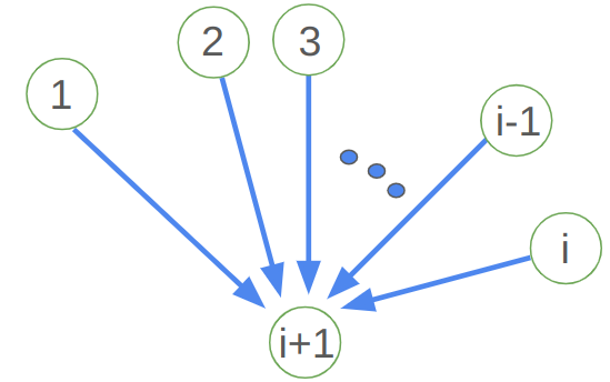
Figure 6: The star graph $D_{i}$ formed by a node with in-degree $i$.

Proposition 4.1.

For $N>\kappa k+1$,

$$Q_{k,j}^{N}=\sum_{i=j}^{\kappa k}(-1)^{i-j}\binom{i}{j}I_{D_{i}}^{N}.$$ (8)

Proof.

Since $D_{i}\subseteq D_{i+1}$, the number of copies of $D_{i}$ in $G_{k}^{N}$ can be written as

$$I_{D_{i}}^{N}=Q_{k,i}^{N}+\binom{i+1}{i}Q_{k,i+1}^{N}+\cdots++\binom{\kappa k}{i}Q_{k,\kappa k+1}^{N}.$$

Stacking these equations into a matrix form for $1\leq i\leq\kappa k$, we obtain

$$\begin{bmatrix}I_{D_{1}}^{N}\\ I_{D_{2}}^{N}\\ \vdots\\ I_{D_{\kappa k-1}}^{N}\\ I_{D_{\kappa k}}^{N}\end{bmatrix}=\begin{bmatrix}1&\binom{2}{1}&\cdots&\binom{\kappa k-1}{1}&\binom{\kappa k}{1}\\ 0&1&\cdots&\binom{\kappa k-1}{2}&\binom{\kappa k}{2}\\ \vdots&\vdots&\ddots&\vdots&\vdots\\ 0&0&\cdots&1&\binom{\kappa k}{\kappa k-1}\\ 0&0&\cdots&0&1\\ \end{bmatrix}\begin{bmatrix}Q_{k,1}^{N}\\ Q_{k,2}^{N}\\ \vdots\\ Q_{k,\kappa k-1}^{N}\\ Q_{k,\kappa k+1}^{N}\end{bmatrix}.$$ (9)

The system of linear equations can be solved for the variables $Q_{k,\cdot}^{N}$ to obtain the statement of the proposition. ∎

Convergence of the variables $I_{D_{i}}^{N}$ is characterized in Theorem 2.1 of [4] which is reproduced below.

Theorem 4.2.

Let $m\geq 1$, $a_{1},\cdots,a_{m}$ be real numbers, $D_{1},\cdots,D_{m}$ be weakly connected directed graphs, and $I^{N}=a_{1}I_{D_{1}}^{N}+a_{2}I_{D_{2}}^{N}+\cdots+a_{m}I_{D_{m}}^{N}$. Then there exist constants $\xi,\tau$ such that as $N\rightarrow\infty$

$$\frac{I^{N}}{N}\rightarrow\xi\hskip 14.22636pt\text{a.s.},\ \hskip 7.11317pt \hskip 7.11317pt\frac{\text{Var}(I^{N})}{N}\rightarrow\tau^{2},\hskip 17.07182pt\text{ and }\hskip 17.07182pt\frac{I^{N}-\mathbb{E}\big{[}I^{N}\big{]}}{\sqrt{N}}\stackrel{{\scriptstyle\text{d}}}{{\rightarrow}}\mathcal{N}(0,\tau^{2}),$$

where $\mathcal{N}(\mu,\sigma^{2})$ denotes the normal distribution with mean $\mu$ and variance $\sigma^{2}$.

As a corollary of Proposition 8 and Theorem 4.2, we obtain the convergence of the random variables $Q_{k,j}^{N}$ as stated below.

Corollary 4.3.

For $0\leq j\leq\kappa k$, there exist constants $q_{j}(d,k)$ and $\tau_{j}^{2}$ such that as $N\rightarrow\infty$

$$\frac{Q_{k,j}^{N}}{N}\rightarrow q_{j}(d,k)\hskip 14.22636pt\text{a.s.},\hskip 7.11317pt\frac{\text{Var}(Q_{k,j}^{N})}{N}\rightarrow\tau_{j}^{2},\hskip 8.5359pt\text{ and }\hskip 8.5359pt\frac{Q_{k,j}^{N}-\mathbb{E}\big{[}Q_{k,j}^{N}\big{]}}{\sqrt{N}}\stackrel{{\scriptstyle\text{d}}}{{\rightarrow}}\mathcal{N}(0,\tau_{j}^{2}).$$

The value of the constant $q_{j}(d,k)$ is hard to compute for general $k$. For the case of $k=1$, [14] shows that

$$q_{j}(d,1)=\frac{1}{j!}\sum_{i=0}^{\kappa-j}\frac{(-1)^{i}}{i!}C_{i+j}^{d},$$ (10)

where

$$C^{d}_{k}\ =\ \int_{A_{k}^{d}}e^{-\text{vol}\big{(}B(u_{1},\|u_{1}\|)\cup\cdots\cup B(u_{k},\|u_{k}\|)\big{)}}du_{1}\dots du_{k},$$

with

$$A_{k}^{d}\ =\ \Big{\{}(u_{1},\dots,u_{k})\in(\mathbb{R}^{d})^{k}\colon\|u_{i}\|<\|u_{j}-u_{i}\|\ \text{for all $i\neq j$}\Big{\}},$$

and $\text{vol}(B)$ denoting the Lebesgue measure of set $B$.

4.3 Analysis of NNS strategies

As in the case of one dimension, we first look at a deterministic strategy and then address the probabilistic NNS strategies. In Section 4.3.1, we look at the oNNS strategy for $k=1$. The results obtained here are used in Sections 4.3.2 and 4.3.3 to obtain the fraction of overloaded servers for the probabilistic NNS strategies.

4.3.1 oNNS strategy

In this strategy, a customer on arriving at a server joins the queue at its nearest neighbour deterministically. The following theorem characterizes the asymptotic load and the fraction of overloaded servers when customers follow the oNNS strategy.

Theorem 4.4.

Consider $N$ servers distributed uniformly in $[0,1]^{d}$ with Poisson arrivals of intensity $\lambda$ following the oNNS strategy. For any $v\in[N]$, the asymptotic load satisfies

$$L_{v}=\lim_{t\rightarrow\infty}\frac{J_{v}(t)}{t}\ \in\ \{0,\lambda,2\lambda,\cdots,\kappa k\lambda\}\hskip 5.69046pt\text{a.s.},$$

and the fraction of overloaded servers

$$\mathcal{O}_{N}\rightarrow\sum_{j=2}^{\kappa k}q_{j}(d,1)\hskip 14.22636pt\text{a.s.}\hskip 14.22636pt\text{ as }N\rightarrow\infty.$$

Proof.

On the routing graph $G_{1}^{N}$, an arrival at node $u$ follows the only outgoing edge $u\longrightarrow v$ and joins the queue at $v$. Arrivals to queues from vertices other than $u$ can also join the queue at $v$ if node $v$ is the nearest neighbour to these vertices. Thus, the in-degree of node $v$ in $G_{1}^{N}$ corresponds to the number of queues whose arrivals join the queue at node $v$. From Property 2 of the routing graph the in-degree is bounded from above by $\kappa k$. Thus, for the oNNS strategy we have that for all $v\in[N]$, the asymptotic load at node $v$ takes values in

$$L_{v}=\lim_{t\rightarrow\infty}\frac{J_{v}(t)}{t}\ \in\ \{0,\lambda,2\lambda,\cdots,\kappa k\lambda\}\hskip 5.69046pt\text{a.s.}$$

Moreover, the servers with an asymptotic load of $m\lambda$ are precisely those nodes in $G_{1}^{N}$ with an in-degree of $m$. In the previous section, we denoted the number of nodes with in-degree $m$ by $Q_{1,m}^{N}$.

A server $v$ is overloaded if its asymptotic load exceeds $\lambda$. For arrivals following the oNNS strategy, the server at $v$ gets overloaded if arrivals from more than one node join it. This happens if the in-degree of node $v$ is greater than $1$ in the routing graph. Thus, the fraction of overloaded servers is

$$\mathcal{O}_{N}=\frac{\sum_{j=2}^{\kappa k}Q_{1,j}^{N}}{N}.$$

Using Corollary 4.3 and the fact that the sum of sequences converging almost surely converges to their sum almost surely, we obtain the characterization of the fraction of overloaded servers, $\mathcal{O}_{N}$, as in the statement of the theorem. ∎

4.3.2 Pure $k$-NNS strategy

In the pure $k$-NNS strategy, we introduce randomness into the oNNS strategy by allowing an arrival to choose one among the $k\geq 2$ nearest neighbour queues with equal probability instead of just joining the nearest one. The load and the fraction of overloaded servers for this strategy is given in the following theorem.

Theorem 4.5.

Consider $N$ servers distributed uniformly in $[0,1]^{d}$ with Poisson arrivals of intensity $\lambda$ following the pure $k$-NNS strategy. For any $v\in[N]$, the asymptotic load satisfies

$$L_{v}\ \in\ \Bigg{\{}0,\frac{\lambda}{k},\frac{2\lambda}{k},\cdots,\kappa\lambda\Bigg{\}}\hskip 28.45274pt\text{a.s..}$$

and the fraction of overloaded servers

$$\mathcal{O}_{N}\rightarrow\sum_{j=k+1}^{\kappa k}q_{j}(d,k)\hskip 14.22636pt\text{a.s.}\hskip 28.45274pt\text{ as }N\rightarrow\infty.$$

Proof.

As in the oNNS case, the in-degree of a node in $G_{k}^{N}$ governs the asymptotic load at the corresponding server. However, since arrivals choose among $k$ possible queues to join, each of the $k$ outgoing edges of a node $u$ in $G_{k}^{N}$ can be associated with a thinned Poisson process of intensity $\frac{\lambda}{k}$. Naturally, every incoming edge in $G_{k}^{N}$ contributes a load proportional to $\frac{\lambda}{k}$. Therefore, the possible asymptotic loads at a node $v$ are

$$L_{v}\ \in\ \Bigg{\{}0,\frac{\lambda}{k},\frac{2\lambda}{k},\cdots,\kappa\lambda\Bigg{\}}\hskip 28.45274pt\text{a.s..}$$

From the structure of the possible asymptotic loads, it is easy to infer that a server gets overloaded if it has an in-degree greater than $k$. Therefore, the fraction of overloaded servers can be expressed as

$$\mathcal{O}_{N}=\frac{\sum_{j=k+1}^{\kappa k}Q_{k,j}^{N}}{N}.$$

Using Corollary 4.3, we obtain the statement of the theorem. ∎

4.3.3 $(k,p)$-NNS strategy

We have now set up the stage to address the $(k,p)$-NNS strategy. The following theorem provides the asymptotic load and the fraction of overloaded servers for arrivals following the $(k,p)$-NNS strategy.

Theorem 4.6.

Consider $N$ servers distributed uniformly in $[0,1]^{d}$ with Poisson arrivals of intensity $\lambda$ following the $(k,p)$-NNS strategy. For any $v\in[N]$, the asymptotic load satisfies

$$L_{v}\in\Bigg{\{}\lambda\left[\frac{j}{k}+\left(1-\frac{j}{k}\right)p\right],j\in\{0,1,\cdots,\kappa k\}\Bigg{\}}\qquad\text{a.s.,}$$

and the fraction of overloaded servers satisfies

$$\mathcal{O}_{N}\rightarrow\sum_{j=k+1}^{\kappa k}q_{j}(d,k)\hskip 14.22636pt\text{a.s.}\hskip 14.22636pt\text{ as }N\rightarrow\infty.$$

Proof.

Similar to the analysis in Section 3.3, we divide the arrivals to server $u$ into active and lazy components denoted by $N^{A}_{u}(t)$ and $N^{L}_{u}(t)$ of intensities $\lambda(1-p)$ and $\lambda p$ respectively. The asymptotic load at node $v$ is the sum of the contributions from the lazy component of node $v$ and active components from all vertices for which node $v$ is one of the $k$ nearest neighbours. The routing graph, $G_{k}^{N}$, contains edges to node $v$ from all vertices for which $v$ is one of the $k$ nearest neighbours. Thus, like in the pure $k$-NNS strategy, the number of active component queues that contribute to the load at node $v$ is equal to the in-degree of $v$.

Denote by $J^{L}_{v}(t)$ the number of customers of $N^{L}_{v}(t)$ joining server $v$ till time $t$, and $J^{A}_{v}(t)$ the number of customers of $N^{A}_{u}(t)$ where $u\longrightarrow v\text{ in }G_{k}^{N}$ joining server $v$ till time $t$. Then, for the lazy component we have that $\lim_{t\rightarrow\infty}\frac{J_{v}^{L}(t)}{t}=p\lambda$ a.s.. For the active component, arrivals behave as in the pure $k$-NNS strategy. Since $N_{u}^{A}(t)$ is a Poisson arrival process of intensity $\lambda(1-p)$, from Theorem 4.5 we have that almost surely

$$\lim_{t\rightarrow\infty}\frac{J_{v}^{A}(t)}{t}\in\Bigg{\{}0,\frac{\lambda(1-p)}{k},\frac{2\lambda(1-p)}{k},\cdots,\frac{\kappa k\lambda(1-p)}{k}\Bigg{\}}.$$

Hence the asymptotic load at server $v$ can take values

$$L_{v} =\lim_{t\rightarrow\infty}\frac{J_{v}(t)}{t}=\lim_{t\rightarrow\infty}\frac{J^{L}_{v}(t)+J^{A}_{v}(t)}{t}$$

$$\in\Bigg{\{}\lambda\left[\frac{j}{k}(1-p)+p\right],j\in\{0,1,\cdots,\kappa k\}\Bigg{\}}\qquad\text{a.s.,}$$

which proves the first part of the theorem.

For $j=0,1,\cdots,\kappa k$, the number of servers with asymptotic load $\lambda\left[\frac{j}{k}+\left(1-\frac{j}{k}\right)p\right]$ is precisely the number of nodes with in-degree $j$ in $G_{k}^{N}$ which we denoted by $Q_{k,j}^{N}$. A server is overloaded if its asymptotic load $L_{v}>\lambda$, which in turn happens when the in-degree of $v$ is greater than $k$. In short,

$$\mathcal{O}_{N}=\frac{\sum_{j=k+1}^{\kappa k}Q_{k,j}^{N}}{N}.$$

Thus, using Corollary 4.3, we obtain the latter part of the theorem. ∎

4.4 Implications for one dimension

For queues in one dimension with arrivals following the $(1,p)$-NNS strategy, the fraction of overloaded servers is given by $\mathcal{O}_{N}=\frac{Q_{1,2}^{N}}{N}$. In Section 3.3, it was found that $\mathbb{E}\mathcal{O}_{N}=\frac{1}{4}$. Theorem 4.6 characterizes the distribution of $\mathcal{O}_{N}$ as $N\rightarrow\infty$ leading to

$$\mathcal{O}_{N}\rightarrow q_{2}(1,1)=\frac{1}{4}\hskip 14.22636pt\text{a.s.}\hskip 14.22636pt\text{ as }N\rightarrow\infty.$$

Note that $N\mathcal{O}_{N}=Q_{1,2}^{N}$ is the number of overloaded servers which from Corollary 4.3 satisfies

$$\frac{Q_{1,2}^{N}}{N}\rightarrow q_{2}(1,1)\hskip 14.22636pt\text{a.s.},\hskip 7.11317pt\frac{\text{Var}(Q_{1,2}^{N})}{N}\rightarrow\tau_{2}^{2},\hskip 8.5359pt\text{ and }\hskip 8.5359pt\frac{Q_{1,2}^{N}-\mathbb{E}\big{[}Q_{1,2}^{N}\big{]}}{\sqrt{N}}\stackrel{{\scriptstyle\text{d}}}{{\rightarrow}}\mathcal{N}(0,\tau_{2}^{2}).$$

The authors in [3] obtain the exact values of these constants to be $q_{2}(1,1)=\frac{1}{4}$ and $\tau_{2}^{2}=\frac{19}{240}$. Thus the number of overloaded servers has a normal distribution in the regime when $N\rightarrow\infty$. This is illustrated in our numerical results in Section 5.

5 Numerical results

In this section, we present simulation experiments justifying our results. We restrict to the case of $k=1$ since the constants in our results (or their approximation using Monte Carlo simulations) are known only for the $(1,p)$-NNS strategy.

Consider $N=1000$ servers deployed uniformly in $[0,1]$, each of which is associated with an independent arrival process of intensity $\lambda=1$. The arrival process is simulated for $t=1000$ time units with each arrival being lazy with probability $p$ or active with probability $1-p$. The probability parameter $p$ is chosen from the set $\{0,0.25,0.5,0.75\}$, where $p=0$ corresponds to the oNNS strategy. Fig. 7a plots the histogram of the observed number of overloaded servers ($NR_{2-p}$) and the servers with no change in load ($NR_{1}$) over $1000$ instantiations of the server locations in the one dimension case. The expected number of overloaded servers is concentrated well around the mean of $N/4=250$ irrespective of the probability $p$ corroborating with Theorem 3.5.

Fig. 7b shows a similar histogram of the expected fraction of overloaded servers when the servers are distributed in $[0,1]^{2}$. The values of the constants $q_{j}(2,1)$ for $j=0,1,\cdots,5$ have been computed using Monte Carlo simulations in [5] which is reproduced in Table 2.

$\bm{j}$	$\bm{q_{j}(2,1)}$
$0$	$0.284$
$1$	$0.463$
$2$	$0.221$
$3$	$3.04\times 10^{-2}$
$4$	$6.56\times 10^{-4}$
$5$	$1.9\times 10^{-7}$
$6$ or more	$0$

Table 2: Values of $q_{j}(2,1)$ for different values of $j$.

When the servers are distributed in $2$D and customers follow the $(1,p)$-NNS strategy, Theorem 4.6 states that the fraction of overloaded servers converges to $\sum_{j=2}^{5}q_{j}(2,1)$ almost surely as $N\rightarrow\infty$. Using the values from Table 2, we obtain $\sum_{j=2}^{5}q_{j}(2,1)\approx 0.252$ which is where the blue peak is located in Fig. 7b. Further supporting the result is the peak observed of the fraction of servers with no change in load which is equal to $q_{1}(2,1)=0.463$.

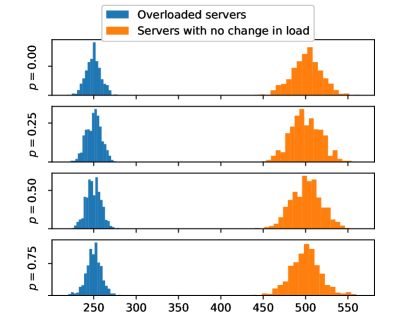
(a) $d=1$

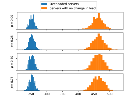
(b) $d=2$

Figure 7: Histogram of the number of overloaded servers and the servers with no change in load for different probability values of the $(1,p)$-NNS strategy in (a) one dimension and (b) two dimension.

6 Conclusions and future work

In this paper, we consider multiple servers on a $d$-dimensional Euclidean space. Each server is associated with a Poisson queue of intensity $\lambda$. Customers in each queue follow a probabilistic policy to either remain in the queue or to join a nearest neighbour. In this setting, we evaluate the fraction of overloaded servers in the stationary regime.

In Section 3, we obtained the expected fraction of overloaded servers in the one dimensional case. While it might seem that the results in Section 4 are much stronger as compared to those in Section 3, it is to be noted that the results for the one-dimensional case are not asymptotic in $N$, but instead hold for every $N$. This is not the case for the results obtained in Section 4. Moreover, it is to be noted that similar computations as in Section 3 can be performed for other distributions of the servers since they rely on just the order statistics.

Numerous questions are yet to be answered in this setting, some of which are listed below:

• What is the distribution of the overloaded servers in space? In the long run, the overloaded servers require higher maintenance compared to other servers and this necessitates a characterization of their distribution in space. Fig. 8 and Fig. 9 show the distribution of the overloaded servers in space in one and two dimensions respectively. This is of particular importance in the context of electric vehicles since it gives a spatial distribution of charging stations requiring maintenance.

  

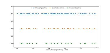
  (a) $p=0$

  

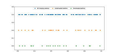
  (b) $p=0.25$

  

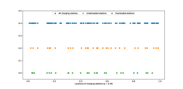
  (c) $p=0.40$

  

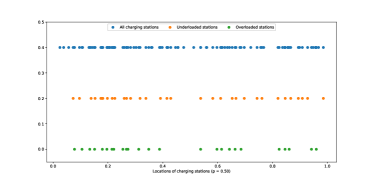
  (d) $p=0.50$

  Figure 8: Spatial distribution of $100$ charging stations (top blue), underloaded stations (middle orange) and overloaded stations (bottom green) in $[0,1]$ for different probability values.

  

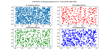
  (a) $p=0$

  

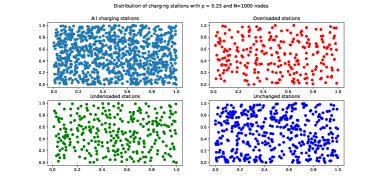
  (b) $p=0.25$

  

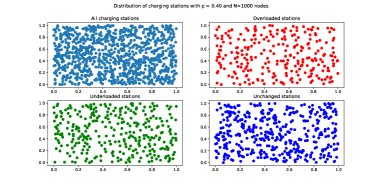
  (c) $p=0.40$

  

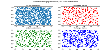
  (d) $p=0.50$

  Figure 9: Spatial distribution of $1000$ charging stations (top-left), overloaded stations (top-right), underloaded stations (bottom-left) and stations with unchanged load (bottom-right) in $[0,1]^{2}$ for different probability values.

• How does $\mathcal{O}_{N}$ behave for strategies where the probability parameters depend on the state of the queue? In this work, we consider the stationary regime for the queues. In contrast, when the shift probabilities depend on transient queue parameters, such as queue length, or on the ambient space, characterization of $\mathcal{O}_{N}$ is an interesting research direction. On a related note, [12, 16] investigate the steady-state behaviour and queue stability when the arrivals are distributed on the circle and a myopic server operates according to a greedy policy serving the nearest arrivals. In our case, however, we have multiple servers. When customers change queues based on the queue length they observe when they arrive, characterization of the steady-state behaviour and queue stability are compelling future directions.

• How does the ambient space impact $\mathcal{O}_{N}$? If factors from the Euclidean space such as traversal times to other queues are considered, several classical queueing problems (delay, wait times etc.) can be formulated which might be interesting in their own right.

It is clear that there are numerous questions that have to be addressed and that there is ample scope for future work.

References

- [1] E. Altman and H. Levy. Queueing in space. Advances in Applied Probability, 26(4):1095–1116, 1994.
- [2] R. Atat, M. Ismail, and E. Serpedin. Stochastic geometry planning of electric vehicles charging stations. In Proc. International Conference on Acoustics, Speech and Signal Processing (ICASSP), pages 3062–3066, May 2020.
- [3] S. Bahadır and E. Ceyhan. On the number of reflexive and shared nearest neighbor pairs in one-dimensional uniform data. arXiv preprint arXiv:1605.01940, 2016.
- [4] S. Bahadır and E. Ceyhan. On the number of weakly connected subdigraphs in random kNN digraphs. Discrete & Computational Geometry, 65(1):116–142, 2021.
- [5] J. Cuzick and R. Edwards. Spatial clustering for inhomogeneous populations. Journal of the Royal Statistical Society Series B: Statistical Methodology, 52(1):73–96, 1990.
- [6] H. A. David and H. N. Nagaraja. Order statistics. John Wiley & Sons, 2004.
- [7] G. Dong, J. Ma, R. Wei, and J. Haycox. Electric vehicle charging point placement optimisation by exploiting spatial statistics and maximal coverage location models. Transportation Research Part D: Transport and Environment, 67:77–88, Feb. 2019.
- [8] S. A. Dudin, O. S. Dudina, and O. I. Kostyukova. Analysis of a queuing system with possibility of waiting customers jockeying between two groups of servers. Mathematics, 11(6):1475, Jan. 2023.
- [9] D. Eppstein, M. S. Paterson, and F. F. Yao. On nearest-neighbor graphs. Discrete & Computational Geometry, 17:263–282, 1997.
- [10] V. Kavitha and E. Altman. Queuing in space: Design of message ferry routes in static ad hoc networks. In 2009 21st International Teletraffic Congress, pages 1–8, Sept. 2009.
- [11] E. Koenigsberg. On jockeying in queues. Management Science, Jan. 1966.
- [12] L. Leskelä and F. Unger. Stability of a spatial polling system with greedy myopic service. Annals of Operations Research, 198:165–183, 2012.
- [13] B. Lin, Y. Lin, and R. Bhatnagar. Optimal policy for controlling two-server queueing systems with jockeying. Journal of Systems Engineering and Electronics, 33(1):144–155, Feb. 2022.
- [14] C. M. Newman, Y. Rinott, and A. Tversky. Nearest neighbors and Voronoi regions in certain point processes. Advances in Applied Probability, 15(4):726–751, 1983.
- [15] C. Ren and Y. Hou. A novel evaluation method of electric vehicles charging network based on stochastic geometry. Oct. 2020. Pages: 468.
- [16] L. T. Rolla and V. Sidoravicius. Stability of the greedy algorithm on the circle. Communications on Pure and Applied Mathematics, 70(10):1961–1986, 2017.
- [17] S. Ross. A first course in probability. Pearson, 2010.
- [18] K. W. Stacey and D. P. Kroese. Greedy servers on a torus. In Proceedings of the 2011 Winter Simulation Conference (WSC), pages 369–380, Dec. 2011.
- [19] G. D. Çelik and E. Modiano. Dynamic vehicle routing for data gathering in wireless networks. In 49th IEEE Conference on Decision and Control (CDC), pages 2372–2377, Dec. 2010.