Testing Calibration in Subquadratic Time

Abstract

In the recent literature on machine learning and decision making, calibration has emerged as a desirable and widely-studied statistical property of the outputs of binary prediction models. However, the algorithmic aspects of measuring model calibration have remained relatively less well-explored. Motivated by [BGHN23a], which proposed a rigorous framework for measuring distances to calibration, we initiate the algorithmic study of calibration through the lens of property testing. We define the problem of calibration testing from samples where given $n$ draws from a distribution $\mathcal{D}$ on $(\text{predictions},\text{binary outcomes})$, our goal is to distinguish between the case where $\mathcal{D}$ is perfectly calibrated, and the case where $\mathcal{D}$ is $\varepsilon$-far from calibration.

We design an algorithm based on approximate linear programming, which solves calibration testing information-theoretically optimally (up to constant factors) in time $O(n^{1.5}\log(n))$. This improves upon state-of-the-art black-box linear program solvers requiring $\Omega(n^{\omega})$ time, where $\omega>2$ is the exponent of matrix multiplication. We also develop algorithms for tolerant variants of our testing problem, and give sample complexity lower bounds for alternative calibration distances to the one considered in this work. Finally, we present preliminary experiments showing that the testing problem we define faithfully captures standard notions of calibration, and that our algorithms scale to accommodate moderate sample sizes.

1 Introduction

Probabilistic predictions are at the heart of modern data science. In domains as wide-ranging as forecasting (e.g. predicting the chance of rain from meteorological data [MW84, Mur98]), medicine (e.g. assessing the likelihood of disease [Doi07]), computer vision (e.g. assigning confidence values for categorizing images [VDDP17]), and more (e.g. speech recognition [AAA⁺16] and recommender systems [RRSK11]), prediction models have by now become essential components of the decision-making pipeline. Particularly in the context of critical, high-risk use cases, the interpretability of prediction models is therefore paramount in downstream applications. That is, how do we assign meaning to the predictions our model gives us, especially when the model is uncertain?

We focus on perhaps the most ubiquitous form of prediction modeling: binary predictions, represented as tuples $(v,y)$ in $[0,1]\times\{0,1\}$ (where the $v$ coordinate is our prediction of the likelihood of an event, and the $y$ coordinate is the observed outcome). We model prediction-outcome pairs in the binary prediction setting by a joint distribution $\mathcal{D}$ over $[0,1]\times\{0,1\}$, fixed in the following discussion. In this context, calibration of a predictor has emerged as a basic desideratum. A prediction-outcome distribution $\mathcal{D}$ is said to be calibrated if

$$\mathbb{E}_{(v,y)\sim\mathcal{D}}[y\mid v=t]=t\text{ for all }t\in[0,1].$$ (1)

That is, calibration asks that the outcome is $1$ exactly $60\%$ of the time, when the model returns a prediction $v=0.6$. While calibration (or approximate variants thereof) is a relatively weak requirement on a meaningful predictor, as it can be achieved by simple models, it can still be significantly violated in practice. For example, interest in calibration in the machine learning community was spurred by [GPSW17], which observed that many modern deep learning models are far from calibrated. Moreover, variants of calibration have been shown to have strong postprocessing properties for fairness constraints and loss minimization [HKRR18, DKR⁺21, GKR⁺22], which has garnered renewed interest in calibration by the theoretical computer science and statistics communities.

The question of measuring the calibration of a distribution is subtle; even a calibrated distribution incurs measurement error due to sampling. For example, consider the expected calibration error, used in e.g. [NCH15, GPSW17, MDR⁺21a, RT21b] as a ground-truth notion of calibration distance:

$$\mathsf{ECE}(\mathcal{D}):=\mathbb{E}_{(v,y)\sim\mathcal{D}}\left[\left|\mathbb{E}_{(v^{\prime},y)\sim\mathcal{D}}\left[y\mid v^{\prime}=v\right]-v\right|\right].$$

Unfortunately, the empirical $\mathsf{ECE}$ is typically meaningless; if the marginal density of $v$ is continuous, we will almost surely only observe a single sample with each $v$ value. Further, [KF08] observed that $\mathsf{ECE}$ is discontinuous in $v$. In practice, binned variants of $\mathsf{ECE}$ are often used as a proxy, where a range of $v$ is lumped together in the conditioning event. However, hyperparameter choices (e.g. the number of bins) can significantly affect the quality of binned $\mathsf{ECE}$ variants as a distance measure [KLM19, NDZ⁺19, MDR⁺21a]. Moreover, as we explore in this paper, binned calibration measures inherently suffer from larger sample complexity-to-accuracy tradeoffs, and are less faithful to ground truth calibration notions in experiments than the calibration distance measures we consider.

Recently, [BGHN23a] undertook a systematic study of various notions of distance to calibration proposed in the literature. They proposed information-theoretic tractability in the prediction-only access (PA) model, where the distance to calibration definition can only depend on the joint prediction-outcome distribution (rather than the features of training examples), as a desirable criterion for calibration distances. Correspondingly, [BGHN23a] introduced Definition 1 as a ground-truth notion of distance to calibration in the PA model, which we also adopt in this work.

Definition 1 (Lower distance to calibration).

Let $\mathcal{D}$ be a distribution over $[0,1]\times\{0,1\}$. The lower distance to calibration (LDTC) of $\mathcal{D}$, denoted ${\underline{\mathsf{dCE}}}(\mathcal{D})$, is defined by

$${\underline{\mathsf{dCE}}}(\mathcal{D}):=\inf_{\Pi\in\textup{ext}(\mathcal{D})}\mathbb{E}_{(u,v,y)\sim\Pi}\left|u-v\right|,$$

where $\textup{ext}(\mathcal{D})$ is all joint distributions $\Pi$ over $(u,v,y)\in[0,1]\times[0,1]\times\{0,1\}$ satisfying the following.

• The marginal distribution of $(v,y)$ is $\mathcal{D}$.

• The marginal distribution $(u,y)$ is perfectly calibrated, i.e. $\mathbb{E}_{\Pi}[y|u]=u$.

Definition 1 has various beneficial aspects: it is convex in $v$, computable in the PA model, and (as shown by [BGHN23a]) polynomially-related to various other calibration distance notions, including some which require feature access. Roughly, the LDTC of a distribution is the tightest lower bound on the $\ell_{1}$ distance between $v$ and any calibrated function of the features which can be made, after taking features into account. The LDTC is the analog of this feature-aware definition of calibration distance when limited to the PA model. We focus on this definition in the remainder of the paper.

1.1 Our results

We initiate the algorithmic study of the calibration testing problem, defined as follows.

Definition 2 (Calibration testing).

Let $\varepsilon\in[0,1]$. We say algorithm $\mathcal{A}$ solves the $\varepsilon$-calibration testing problem with $n$ samples, if given $n$ i.i.d. draws from a distribution $\mathcal{D}$ over $[0,1]\times\{0,1\}$, $\mathcal{A}$ returns either “yes” or “no” and satisfies the following with probability $\geq\frac{2}{3}$.

• $\mathcal{A}$ returns “no” if ${\underline{\mathsf{dCE}}}(\mathcal{D})\geq\varepsilon$.

• $\mathcal{A}$ returns “yes” if ${\underline{\mathsf{dCE}}}(\mathcal{D})=0$.

In this case, we also call $\mathcal{A}$ an $\varepsilon$-calibration tester.

To our knowledge, we are the first work to formalize the calibration testing problem. Definition 2 is natural from the perspective of property testing, an influential paradigm in statistical learning [Ron08, Ron09, Gol17]. In particular, there is an $\varepsilon_{n}=\Theta(n^{-1/2})$ so that it is information-theoretically impossible to solve the $\varepsilon_{n}$-calibration testing problem from $n$ samples (see Lemma 2), so a variant of Definition 2 with an exact distinguishing threshold between “calibrated/uncalibrated” is not tractable. Hence, Definition 2 only requires distinguishing distributions $\mathcal{D}$ which are “clearly uncalibrated” (parameterized by a threshold $\varepsilon$) from those which are perfectly calibrated.

Our first algorithmic contribution is a subquadratic-time algorithm for calibration testing, in the regime where the threshold $\varepsilon$ is information-theoretically optimal up to a constant.

Theorem 1 (Informal, see Theorem 3, Corollary 3).

Let $n\in\mathbb{N}$, and let $\varepsilon=\Omega(\varepsilon_{n})$, where $\varepsilon_{n}=\Theta(n^{-1/2})$ is minimal such that it is information-theoretically possible to solve the $\varepsilon_{n}$-calibration testing problem with $n$ samples. There is an algorithm which solves the $\varepsilon$-calibration testing problem with $n$ samples, running in time $O(\frac{n\log(n)}{\varepsilon})=O(n^{1.5}\log(n))$.

We prove Theorem 1 by designing an algorithm for estimating ${\mathsf{smCE}}(\widehat{\mathcal{D}}_{n})$, the smooth calibration error (Definition 3), an alternative calibration distance measure, of an empirical distribution $\widehat{\mathcal{D}}_{n}$.

Definition 3 (Smooth calibration error).

Let $W$ be the set of Lipschitz functions $w:[0,1]\to[-1,1]$. The smooth calibration error of distribution $\mathcal{D}$ over $[0,1]\times\{0,1\}$, denoted ${\mathsf{smCE}}(\mathcal{D})$, is defined by

$${\mathsf{smCE}}(\mathcal{D})=\sup_{w\in W}\left|\mathbb{E}_{(v,y)\sim\mathcal{D}}[(y-v)w(v)]\right|.$$

It was shown in [BGHN23a] that ${\mathsf{smCE}}(\mathcal{D})$ is a constant-factor approximation to ${\underline{\mathsf{dCE}}}(\mathcal{D})$ for all $\mathcal{D}$ on $[0,1]\times\{0,1\}$ (see Lemma 12). Additionally, the empirical ${\mathsf{smCE}}$ admits a representation as a linear program with an $O(n)\times O(n)$-sized constraint matrix encoding Lipschitz constraints. Thus, [BGHN23a] proposed a simple procedure for estimating ${\mathsf{smCE}}(\mathcal{D})$: draw $n$ samples from $\mathcal{D}$, and solve the associated linear program on the empirical distribution. While there have been significant recent runtime advances in the linear programming literature [LS14, CLS21, vdBLSS20, vdBLL⁺21], all state-of-the-art black-box linear programming algorithms solve linear systems involving the constraint matrix, which takes $\Omega(n^{\omega})$ time, where $\omega>2.371$ [WXXZ23] is the current exponent of matrix multiplication. Even under the best-possible assumption that $\omega=2$, the strategy of exactly solving a linear program represents an $\Omega(n^{2})$ quadratic runtime barrier for calibration testing.

Our work bypasses this barrier by noting that it suffices to solve the ${\mathsf{smCE}}$ linear program to low accuracy, i.e. $\varepsilon=\Omega(n^{-1/2})$, making it amenable to approximate (first-order method based) solvers. However, the ${\mathsf{smCE}}$ linear program (see (11)) is hard-constrained, so standard first-order methods do not readily apply. We develop a novel approximate solver based on a custom combinatorial rounding procedure, used to argue about the error incurred by lifting the smooth calibration constraints into a penalty term, making it amenable to existing minimax optimization procedures. Our algorithm proving the runtime bound in Theorem 1 is given in Section 3.

We next define a tolerant variant of Definition 2 (see Definition 4), where we allow for error thresholds in both the “yes” and “no” cases; “yes” is the required answer when ${\underline{\mathsf{dCE}}}(\mathcal{D})\leq\varepsilon_{2}$, and “no” is required when ${\underline{\mathsf{dCE}}}(\mathcal{D})\geq\varepsilon_{1}$. Our algorithm in Theorem 1 continues to serve as an efficient tolerant calibration tester when $\varepsilon_{1}\geq 4\varepsilon_{2}$, with formal guarantees stated in Theorem 3. This constant-factor loss comes from a similar loss in the relationship between ${\mathsf{smCE}}$ and ${\underline{\mathsf{dCE}}}$, see Lemma 12. We make the observation that a constant factor loss in the tolerant testing parameters is inherent following this strategy, via a lower bound in Lemma 13. Thus, even given infinite samples, computing the smooth calibration error cannot solve tolerant calibration testing all the way down to the information-theoretic threshold $\varepsilon_{1}\geq\varepsilon_{2}$. To develop an improved tolerant calibration tester, we directly show how to approximate the LDTC of an empirical distribution, our second main algorithmic contribution.

Theorem 2 (Informal, see Theorem 4, Corollary 4).

Let $n\in\mathbb{N}$, and let $\varepsilon_{1}-\varepsilon_{2}=\Omega(\varepsilon_{n})$, where $\varepsilon_{n}=\Theta(n^{-1/2})$ is minimal such that it is information-theoretically possible to solve the $\varepsilon_{n}$-calibration testing problem with $n$ samples. There is an algorithm which solves the $(\varepsilon_{1},\varepsilon_{2})$-tolerant calibration testing problem with $n$ samples, running in time $O(\frac{n\log(n)}{(\varepsilon_{1}-\varepsilon_{2})^{2}})=O(n^{2}\log(n))$.

While our algorithm in Theorem 2 is slower than that in Theorem 1, it directly approximates the LDTC, rather than a related quantity. We mention that state-of-the-art black-box linear programming based solvers, while still applicable to (a discretized variant of) the empirical LDTC, require $\Omega(n^{2.5})$ time [vdBLL⁺21]. This is because the constraint matrix for the $\varepsilon$-approximate empirical LDTC linear program has dimensions $O(\frac{n}{\varepsilon})\times O(n)$, resulting in a runtime overhead of $\approx\frac{1}{\varepsilon}=O(\sqrt{n})$ in both our approach and more direct solvers. We prove Theorem 2 in Section 4.

In Section 5, we complement our algorithmic results with lower bounds (Theorems 5, 6) on the sample complexity required to solve variants of the testing problem in Definition 2, when ${\underline{\mathsf{dCE}}}$ is replaced with different calibration distances. For several widely-used distances in the machine learning literature, including binned and convolved variants of $\mathsf{ECE}$ [NCH15, BN23], we show that $\widetilde{\Omega}(\varepsilon^{-2.5})$ samples are required to the associated $\varepsilon$-calibration testing problem. This demonstrates a statistical advantage of our focus on ${\underline{\mathsf{dCE}}}$ as our ground-truth notion for calibration testing.

We corroborate our theoretical findings with preliminary experimental evidence on real and synthetic data in Section 6. First, on a simple Bernoulli example, we show that ${\underline{\mathsf{dCE}}}$ and ${\mathsf{smCE}}$ testers are more reliable indicators of calibration distance than a recently-proposed binned $\mathsf{ECE}$ variant. We then apply our ${\mathsf{smCE}}$ tester to postprocessed neural network predictions to test their calibration levels, validating against the findings in [GPSW17]. Finally, we implement our iterative method from Theorem 1 on our Bernoulli dataset, showing that it scales to moderate dimensions and achieves the expected convergence rate. We note that a current limitation of our work is optimizing the implementation to scale more effectively to high dimensions, an important open direction.

1.2 Our techniques

Theorem 1 and Theorem 2 follow from designing custom first-order methods for approximating empirical linear programs associated with the ${\mathsf{smCE}}$ and ${\underline{\mathsf{dCE}}}$ of a sampled dataset $\widehat{\mathcal{D}}_{n}:=\{(v_{i},y_{i})\}_{i\in[n]}\sim_{\textup{i.i.d.}}\mathcal{D}$. In both cases, known generalization bounds from [BGHN23a] show it suffices to approximate the value of the empirical calibration distances to error $\varepsilon=\Omega(n^{-1/2})$.

We begin by explaining our strategy for estimating ${\mathsf{smCE}}(\widehat{\mathcal{D}}_{n})$ (Definition 3). By definition, the smooth calibration error of $\widehat{\mathcal{D}}_{n}$ can be formulated as a linear program,

$$\min_{x\in[-1,1]^{n}}\frac{1}{n}\sum_{i\in[n]}x_{i}(v_{i}-y_{i}),\text{ where }|x_{i}-x_{j}|\leq|v_{i}-v_{j}|\text{ for all }(i,j)\in[n]\times[n].$$ (2)

Here, $x_{i}\in[-1,1]$ corresponds to the weight on $v_{i}$, and there are $2\binom{n}{2}$ constraints on the decision variable $x$, each of which corresponds to a Lipschitz constraint. We can write (2) as an inequality-constrained linear program $\max_{x\in[-1,1]^{n}:\mathbf{A}x\leq b}\left\langle c,x\right\rangle$, for appropriate $\mathbf{A},b,c$. While first-order methods (e.g. Frank-Wolfe type algorithms) can sometimes apply to hard-constrained linear programs, it is unclear how to implement projection steps onto the Lipschitz constraints $\mathbf{A}x\leq b$ in our setting. We instead follow an “augmented Lagrangian” method where we lift the constraints directly into the objective as a soft-constrained penalty term. To prove correctness of this lifting, we follow a line of results in combinatorial optimization [She13, JST19]. These works develop a “proof-by-rounding algorithm” framework to show that the hard-constrained and soft-constrained linear programs have equal values. This rounding-based framework is summarized in Section 2.2 (see Lemma 3).

To use this rounding-based framework, our key technical innovation is showing that if $x$ violates each of a carefully-selected set $S$ of $O(n)$ Lipschitz constraints by at most $\Delta$, we can design a procedure which produces $x^{\prime}$ with $\left\lVert x^{\prime}-x\right\rVert_{\infty}=O(\Delta)$, yet $x^{\prime}$ is fully feasible for the constraints $\mathbf{A}x^{\prime}\leq b$. Our set $S$ is a multilayer construction, stated formally in (20). Informally, we begin by sorting $v$ into nonincreasing order, and defining a “zeroth-layer” of constraints by enforcing the Lipschitz condition on all pairs $(i,i+1)$ for $i\in[n-1]$. The triangle inequality shows that exactly enforcing these constraints suffices for feasibility of the linear program (Lemma 7). Enforcing these zeroth-layer constraints only approximately, however, degrades poorly under iterative rounding. Accordingly, we build three dyadic trees of constraints to protect how much our rounding procedure can iteratively degrade constraint violations. After proving correctness of our rounding method for the smooth calibration error linear program, we use it to show that the soft-constrained objective

$$\min_{x\in[-1,1]^{n}}\left\langle c,x\right\rangle+\left\lVert\max\left(\mathbf{A}_{S:}x-b_{S},\mathbb{0}_{S}\right)\right\rVert_{\infty}$$ (3)

has the same value as (2), for $\mathbf{A},b,c$ from the ${\mathsf{smCE}}$ linear program, and where subscripting by $S$ restricts to only the relevant rows of the matrix $\mathbf{A}$, and the relevant coordinates of $b$. Finally, we apply a recent first-order minimax optimization algorithm of [JT23] to solve the problem (3).

Our high-level approach to proving Theorem 2 is analogous, going through the same rounding-based augmented Lagrangian framework as described before. However, the empirical ${\underline{\mathsf{dCE}}}$ linear program (see Lemma 16) is more complicated than that for ${\mathsf{smCE}}$ error, and imposes two sets of constraints, roughly corresponding to marginal satisfaction of $(v,y)$ and calibration of $(u,y)$ (using notation from Definition 1). We design a two-step rounding procedure, which first fixes the marginals on the $(v,y)$ coordinates, and then calibrates the $u$ coordinates without affecting any $(v,y)$ marginal. One interesting feature of our ${\underline{\mathsf{dCE}}}$ rounding algorithm, compared to prior works [She13, JST19], is that it is cost-sensitive: we take into account the metric structure of the linear costs $c$ to argue rounding does not harm the objective value, rather than naïvely applying Hölder’s inequality.

Finally, our sample complexity lower bounds in Section 5 for alternative calibration measures follow from an information-theoretic analysis using LeCam’s two-point method [LeC73] and Ingster’s method [IS03]. We construct a perfectly-calibrated distribution as well as a family of miscalibrated distributions with large calibration error ($\geq\varepsilon$) in the alternative calibration measures (convolved ECE and interval CE). A testing algorithm for these measures needs to distinguish these two cases. We show that the distinguishing task has high sample complexity ($\approx\varepsilon^{-2.5}$) by bounding the total variation distance between the two joint distributions of the input examples from the two cases. Our proof is inspired by a similar analysis showing a sample complexity lower bound for identity testing in the distribution testing literature (see e.g. Section 3.1 of [Can22]).

1.3 Related work

The calibration performance of deep neural networks has been studied extensively in the literature (e.g. [GPSW17, MDR⁺21b, Rt21a, BGHN23b]). Measuring the calibration error in a meaningful way can be challenging, especially when the predictions are not naturally discretized (e.g. in neural networks). Recently, [BGHN23a] addresses this challenge using the distance to calibration as a central notion. They consider a calibration measure to be consistent if it is polynomially-related to the distance to calibration. Consistent calibration measures include the smooth calibration error [KF04], Laplace kernel calibration error [KSJ18], interval calibration error [BGHN23a], and convolved ECE [BN23]. On the algorithmic front, substantial observations were made by [BGHN23a] on linear programming characterizations of calibration distances such as the LDTC and smooth calibration. While there have been significant advances on the runtime frontier of linear programming solvers, current runtimes for handling an $n\times d$ linear program constraint matrix with $n\geq d$ remain $\Omega(\min(nd+d^{2.5},n^{\omega}))$ [CLS21, vdBLL⁺21]. Our constraint matrix is roughly-square and highly-sparse, so it is plausible that e.g. the recent research on sparse linear system solvers [PV21, Nie22] could apply to the relevant Newton’s method subproblems and improve upon these rates. Moreover, while efficient estimation algorithms have been proposed by [BGHN23a] for (surrogate) interval calibration error and by [BN23] for convolved ECE, these algorithms require suboptimal sample complexity for solving our testing task in Definition 2 (see Section 5). To compute their respective distances to error $\varepsilon$ from samples, these algorithms require $\Omega(\varepsilon^{-5})$ and $\Omega(\varepsilon^{-3})$ time. As comparison, under this parameterization Theorems 1 and 2 require $\widetilde{O}(\varepsilon^{-3})$ and $\widetilde{O}(\varepsilon^{-4})$ time, but can solve stronger testing problems with the same sample complexity, experimentally validated in Section 6.

2 Preliminaries

2.1 Notation

Throughout this paper, we use $\mathcal{D}$ to denote a distribution over $[0,1]\times\{0,1\}$. When $\mathcal{D}$ is clear from context, we let $\widehat{\mathcal{D}}_{n}=\{(v_{i},y_{i})\}_{i\in[n]}$ denote a dataset of $n$ independent samples from $\mathcal{D}$ and, in a slight abuse of notation, the distribution with probability $\frac{1}{n}$ for each $(v_{i},y_{i})$. We say $\mathsf{d}$ is a calibration distance if it takes distributions on $[0,1]\times\{0,1\}$ to the nonnegative reals $\mathbb{R}_{\geq 0}$, so ${\underline{\mathsf{dCE}}}$ (Definition 1) and ${\mathsf{smCE}}$ (Definition 3) are both calibration distances.

When applied to a vector, we let $\left\lVert\cdot\right\rVert_{p}$ denote the $\ell_{p}$ norm for $p\geq 1$. We denote $[n]:=\{i\in\mathbb{N}\mid i\leq n\}$. We let $\mathbb{0}_{d}$ and $\mathbbm{1}_{d}$ denote the all-zeroes and all-ones vectors in dimension $d$. We let $\Delta^{d}:=\{x\in\mathbb{R}^{d}_{\geq 0}\mid\left\lVert x\right\rVert_{1}=1\}$ denote the probability simplex in dimension $d$. The $i^{\text{th}}$ coordinate basis vector is denoted $e_{i}$. We say $\tilde{x}\in\mathbb{R}$ is an $\varepsilon$-additive approximation of $x\in\mathbb{R}$ if $|\tilde{x}-x|\leq\varepsilon$. For a set $S\subset\mathbb{R}$, we say another set $T\subset\mathbb{R}$ is an $\varepsilon$-cover of $S$ if for all $s\in S$, there is $t\in T$ with $|s-t|\leq\varepsilon$. We use $\widetilde{O}$ and $\widetilde{\Omega}$ to hide polylogarithmic factors in the argument.

We denote matrices in boldface throughout. For any matrix $\mathbf{A}\in\mathbb{R}^{m\times n}$, we refer to its $i^{\text{th}}$ row by $\mathbf{A}_{i:}$ and its $j^{\text{th}}$ column by $\mathbf{A}_{:j}$. Moreover, for a set $S$ identified with rows of a matrix $\mathbf{A}$, we let $\mathbf{A}_{s:}$ denote the row indexed by $s\in S$, and use similar notation for columns.

For any $p,q\geq 1$, we define

$$\left\lVert\mathbf{A}\right\rVert_{p\to q}:=\max_{x\in\mathbb{R}^{n}\mid\left\lVert x\right\rVert_{p}\leq 1}\left\lVert\mathbf{A}x\right\rVert_{q}.$$

Notice that in particular, $\left\lVert\mathbf{A}\right\rVert_{1\to 1}$ is the largest $\ell_{1}$ norm of any column of $\mathbf{A}$, and $\left\lVert\mathbf{A}\right\rVert_{\infty\to\infty}$ is the largest $\ell_{1}$ norm of any row. We say that $x\in\mathcal{X}$ is an $\varepsilon$-approximate minimizer of $f:\mathcal{X}\to\mathbb{R}$ if $f(x)-\min_{x^{\prime}\in\mathcal{X}}f(x^{\prime})\leq\varepsilon$. We call $(x,y)\in\mathcal{X}\times\mathcal{Y}$ an $\varepsilon$-approximate saddle point to a convex-concave function $f:\mathcal{X}\times\mathcal{Y}\to\mathbb{R}$ if its duality gap is at most $\varepsilon$, i.e.

$$\max_{y^{\prime}\in\mathcal{Y}}f(x,y^{\prime})-\min_{x^{\prime}\in\mathcal{X}}f(x^{\prime},y)\leq\varepsilon.$$

The following simple claim will often be useful.

Lemma 1.

Let $f:\mathcal{X}\times\mathcal{Y}\to\mathbb{R}$ be convex-concave for compact $\mathcal{X},\mathcal{Y}$, and let $g(x):=\max_{y\in\mathcal{Y}}f(x,y)$ for $x\in\mathcal{X}$. If $(x,y)$ is an $\varepsilon$-approximate saddle point to $f$, $x$ is an $\varepsilon$-approximate minimizer to $g$.

Proof.

Let $y^{\prime}:=\textup{argmax}_{y\in\mathcal{Y}}f(x,y)$ and $x^{\prime}:=\textup{argmin}_{x^{\prime}\in\mathcal{X}}f(x^{\prime},y)$. The conclusion follows from

$$\min_{x^{\star}\in\mathcal{X}}g(x^{\star})=\min_{x^{\star}\in\mathcal{X}}\max_{y^{\star}\in\mathcal{Y}}f(x^{\star},y^{\star})=\max_{y^{\star}\in\mathcal{Y}}\min_{x^{\star}\in\mathcal{X}}f(x^{\star},y^{\star})\geq\min_{x^{\prime}\in\mathcal{X}}f(x^{\prime},y),$$

where we used strong duality (via Sion’s minimax theorem), so that

$$g(x)-\min_{x^{\star}\in\mathcal{X}}g(x^{\star})\leq g(x)-f(x^{\prime},y)=f(x,y^{\prime})-f(x^{\prime},y)\leq\varepsilon.$$

∎

We next define a tolerant variant of the calibration testing problem in Definition 2.

Definition 4 (Tolerant calibration testing).

Let $0\leq\varepsilon_{2}\leq\varepsilon_{1}\leq 1$. We say algorithm $\mathcal{A}$ solves the $(\varepsilon_{1},\varepsilon_{2})$-tolerant calibration testing problem with $n$ samples, if given $n$ i.i.d. draws from a distribution $\mathcal{D}$ over $[0,1]\times\{0,1\}$, $\mathcal{A}$ returns either “yes” or “no” and satisfies the following with probability $\geq\frac{2}{3}$.

• $\mathcal{A}$ returns “no” if ${\underline{\mathsf{dCE}}}(\mathcal{D})\geq\varepsilon_{1}$.

• $\mathcal{A}$ returns “yes” if ${\underline{\mathsf{dCE}}}(\mathcal{D})\leq\varepsilon_{2}$.

In this case, we also call $\mathcal{A}$ an $(\varepsilon_{1},\varepsilon_{2})$-tolerant calibration tester.

Note that an algorithm which solves the $(\varepsilon_{1},\varepsilon_{2})$-tolerant calibration testing problem with $n$ samples also solves the $\varepsilon_{1}$-calibration testing problem with the same sample complexity. Moreover, we give a simple impossibility result on parameter ranges for calibration testing.

Lemma 2.

Let $0\leq\varepsilon_{2}\leq\varepsilon_{1}\leq\frac{1}{2}$ satisfy $\varepsilon_{1}-\varepsilon_{2}=\varepsilon$. There is a universal constant $C_{\textup{coin}}$ such that, given $n\leq\frac{C_{\textup{coin}}}{\varepsilon^{2}}$ samples from a distribution on $[0,1]\times\{0,1\}$, it is information-theoretically impossible to solve the $(\varepsilon_{1},\varepsilon_{2})$-tolerant calibration testing problem.

Proof.

Suppose $\varepsilon\leq\frac{1}{10}$, else we can choose $C_{\textup{coin}}$ small enough such that $n<1$. We consider two distributions over $[0,1]\times\{0,1\}$, $\mathcal{D}$ and $\mathcal{D}^{\prime}$, with ${\underline{\mathsf{dCE}}}(\mathcal{D})\geq\varepsilon_{1}$ but ${\underline{\mathsf{dCE}}}(\mathcal{D}^{\prime})\leq\varepsilon_{2}$, so if $\mathcal{A}$ succeeds at tolerant calibration testing for both $\mathcal{D}$ and $\mathcal{D}^{\prime}$, we must have $\mathrm{d_{TV}}(\mathcal{D}^{\otimes n},(\mathcal{D}^{\prime})^{\otimes n})\geq\frac{1}{3}$, where we denote the $n$-fold product of a distribution with $\cdot^{\otimes n}$. Else, $\mathcal{A}$ cannot return different answers from $n$ samples with probability $\geq\frac{2}{3}$, as required by Definition 4. Specifically, we define $\mathcal{D},\mathcal{D}^{\prime}$ as follows.

• To draw $(v,y)\sim\mathcal{D}$, let $v=\frac{1}{2}+\varepsilon_{1}$ and $y\sim\textup{Bern}(\frac{1}{2})$.

• To draw $(v,y)\sim\mathcal{D}^{\prime}$, let $v=\frac{1}{2}+\varepsilon_{1}$ and $y\sim\textup{Bern}(\frac{1}{2}+\varepsilon)$.

We claim that ${\underline{\mathsf{dCE}}}(\mathcal{D})=\varepsilon_{1}$. To see this, let $\Pi\in\textup{ext}(\mathcal{D})$ and $(u,v,y)\sim\Pi$, so $\mathbb{E}_{(u,v,y)\sim\Pi}[u]=\frac{1}{2}$ because $u$ is calibrated. By Jensen’s inequality, we have:

$$\mathbb{E}_{(u,v,y)\sim\Pi}\left[|u-v|\right]\geq\left|\mathbb{E}_{(u,v,y)\sim\Pi}\left[u\right]-\left(\frac{1}{2}+\varepsilon_{1}\right)\right|=\varepsilon_{1}.$$

The equality case is realized when $u=\frac{1}{2}$ with probability $1$, proving the claim. Similarly, ${\underline{\mathsf{dCE}}}(\mathcal{D}^{\prime})=\varepsilon_{2}$. Finally, let $\pi:=\textup{Bern}(\frac{1}{2})$, $\pi^{\prime}:=\textup{Bern}(\frac{1}{2}+\varepsilon)$, and $\pi^{\otimes n},(\pi^{\prime})^{\otimes n}$ denote their $n$-fold product distributions. Pinsker’s inequality shows that it suffices to show that $d_{\textup{KL}}(\pi^{\otimes n}\|(\pi^{\prime})^{\otimes n})\leq\frac{1}{5}$ to contradict our earlier claim $\mathrm{d_{TV}}((\mathcal{D})^{\otimes n},(\mathcal{D}^{\prime})^{\otimes n})\geq\frac{1}{3}$. To this end, we have

$$d_{\textup{KL}}(\pi^{\otimes n}\|(\pi^{\prime})^{\otimes n}) =n\cdot d_{\textup{KL}}\left(\pi\|\pi^{\prime}\right)=\frac{n}{2}\left(\log\left(\frac{\frac{1}{2}}{\frac{1}{2}+\varepsilon}\right)+\log\left(\frac{\frac{1}{2}}{\frac{1}{2}-\varepsilon}\right)\right)$$

$$=\frac{n}{2}\log\left(\frac{1}{1-4\varepsilon^{2}}\right)\leq\frac{n}{2}\cdot 5\varepsilon^{2}\leq\frac{1}{5},$$

where the first line used tensorization of $d_{\textup{KL}}$, and the last chose $C_{\textup{coin}}$ small enough. ∎

We also generalize Definitions 2 and 4 to apply to an arbitrary calibration distance.

Definition 5 ($\mathsf{d}$ testing).

Let $\mathsf{d}$ be a calibration distance. For $\varepsilon\in\mathbb{R}_{\geq 0}$, we say algorithm $\mathcal{A}$ solves the $\varepsilon$-$\mathsf{d}$-testing problem (or, $\mathcal{A}$ is an $\varepsilon$-$\mathsf{d}$ tester) with $n$ samples, if given $n$ i.i.d. draws from a distribution $\mathcal{D}$ over $[0,1]\times\{0,1\}$, $\mathcal{A}$ returns either “yes” or “no” and satisfies the following with probability $\geq\frac{2}{3}$.

1. $\mathcal{A}$ returns “no” if $\mathsf{d}(\mathcal{D})\geq\varepsilon$.

2. $\mathcal{A}$ returns “yes” if $\mathsf{d}(\mathcal{D})=0$.

For $0\leq\varepsilon_{2}\leq\varepsilon_{1}$, we say algorithm $\mathcal{A}$ solves the $(\varepsilon_{1},\varepsilon_{2})$-tolerant $\mathsf{d}$ testing problem (or, $\mathcal{A}$ is an $(\varepsilon_{1},\varepsilon_{2})$-tolerant $\mathsf{d}$ tester) with $n$ samples, if given $n$ i.i.d. draws from a distribution $\mathcal{D}$ over $[0,1]\times\{0,1\}$, $\mathcal{A}$ returns either “yes” or “no” and satisfies the following with probability $\geq\frac{2}{3}$.

1. $\mathcal{A}$ returns “no” if $\mathsf{d}(\mathcal{D})\geq\varepsilon_{1}$.

2. $\mathcal{A}$ returns “yes” if $\mathsf{d}(\mathcal{D})\leq\varepsilon_{2}$.

2.2 Rounding linear programs

In this section, we give a general framework for approximately solving linear programs, following similar developments in the recent combinatorial optimization literature [She13, JST19]. Roughly speaking, this framework is a technique for losslessly converting a constrained convex program to an unconstrained one, provided we can show existence of a rounding procedure compatible with the constrained program in an appropriate sense. We begin with our definition of a rounding procedure.

Definition 6 (Rounding procedure).

Consider a convex program defined on the intersection of convex set $\mathcal{X}$ with linear equality constraints $\mathbf{A}x=b$:

$$\min_{\begin{subarray}{c}x\in\mathcal{X}\\ \mathbf{A}x=b\end{subarray}}c^{\top}x.$$ (4)

We say $\mathsf{Round}$ is a $(\widetilde{\mathbf{A}},\tilde{b},p)$-equality rounding procedure for $(\mathbf{A},b,c,\mathcal{X})$ if $p\geq 1$, and for any $x\in\mathcal{X}$, there exists $x^{\prime}:=\mathsf{Round}(x)\in\mathcal{X}$ such that $\mathbf{A}x^{\prime}=b$, $\widetilde{\mathbf{A}}x^{\prime}=\tilde{b}$, and

$$c^{\top}x^{\prime}\leq c^{\top}x+\left\lVert\widetilde{\mathbf{A}}x-\tilde{b}\right\rVert_{p}.$$ (5)

Similarly, consider a program on the intersection of a convex set with linear inequality constraints:

$$\min_{\begin{subarray}{c}x\in\mathcal{X}\\ \mathbf{A}x\leq b\end{subarray}}c^{\top}x.$$ (6)

We say $\mathsf{Round}$ is a $(\widetilde{\mathbf{A}},\tilde{b},p)$-inequality rounding procedure for $(\mathbf{A},b,c,\mathcal{X})$ if $p\geq 1$, and for any $x\in\mathcal{X}$, there exists $x^{\prime}:=\mathsf{Round}(x)\in\mathcal{X}$ such that $\mathbf{A}x^{\prime}\leq b$, $\widetilde{\mathbf{A}}x^{\prime}\leq\tilde{b}$, and

$$c^{\top}x^{\prime}\leq c^{\top}x+\left\lVert\max\left(\widetilde{\mathbf{A}}x-\tilde{b},\mathbb{0}_{m}\right)\right\rVert_{p},$$ (7)

where $m$ is the number of rows in $\widetilde{\mathbf{A}}$, $\tilde{b}$, and the $\max$ operation is entrywise.

Intuitively, rounding procedures replace the hard-constrained problems (4), (6) with their soft-constrained variants, i.e. the soft equality-constrained

$$\min_{x\in\mathcal{X}}c^{\top}x+\left\lVert\widetilde{\mathbf{A}}x-\tilde{b}\right\rVert_{p},$$ (8)

and the soft inequality-constrained

$$\min_{x\in\mathcal{X}}c^{\top}x+\left\lVert\max\left(\widetilde{\mathbf{A}}x-\tilde{b},\mathbb{0}_{m}\right)\right\rVert_{p},$$ (9)

respectively, for some $(\widetilde{\mathbf{A}},\tilde{b},p)$ constructed from the hard-constrained problem instance (parameterized by $\mathbf{A},b,c,\mathcal{X}$). Leveraging the assumptions on our rounding procedure in each case (5), (7), we now show how to relate approximate solutions to these problems, generalizing Lemma 1 of [JST19].

Lemma 3.

Let $x$ be an $\varepsilon$-approximate minimizer to (8), and let $\mathsf{Round}$ be a $(\widetilde{\mathbf{A}},\tilde{b},p)$-equality rounding procedure for $(\mathbf{A},b,c,\mathcal{X})$. Then $x^{\prime}:=\mathsf{Round}(x)$ is an $\varepsilon$-approximate minimizer to (4). Similarly, if $x$ is an $\varepsilon$-approximate minimizer to (9) and $\mathsf{Round}$ is a $(\widetilde{\mathbf{A}},\tilde{b},p)$-inequality rounding procedure for $(\mathbf{A},b,c,\mathcal{X})$, $x^{\prime}:=\mathsf{Round}(x)$ is an $\varepsilon$-approximate minimizer to (6).

Proof.

We only discuss the equality-constrained setting (4), (8), as the proof of the inequality-constrained setting is entirely analogous. We first claim that a minimizing solution to (8) satisfies the constraints $\mathbf{A}x=b$. To see this, given any $x\in\mathcal{X}$, we can produce $x^{\prime}\in\mathcal{X}$ with $\mathbf{A}x^{\prime}=b$ and such that $x^{\prime}$ has smaller objective value in (8). Indeed, letting $x^{\prime}:=\mathsf{Round}(x^{\prime})$, (5) guarantees

$$c^{\top}x^{\prime}=c^{\top}x^{\prime}+\left\lVert\widetilde{\mathbf{A}}x^{\prime}-\tilde{b}\right\rVert_{p}\leq c^{\top}x+\left\lVert\widetilde{\mathbf{A}}x-\tilde{b}\right\rVert_{p},$$

as claimed. Now let $x^{\star}\in\mathcal{X}$ satisfying $\mathbf{A}x^{\star}=b$ minimize (8). Then, if $x$ is an $\varepsilon$-approximate minimizer to (8) and $x^{\prime}=\mathsf{Round}(x)$, we have the desired claim from $\mathbf{A}x^{\prime}=b$, and

$$c^{\top}x^{\prime}=c^{\top}x^{\prime}+\left\lVert\widetilde{\mathbf{A}}x^{\prime}-\tilde{b}\right\rVert_{p}\leq c^{\top}x+\left\lVert\widetilde{\mathbf{A}}x-\tilde{b}\right\rVert_{p}\leq c^{\top}x^{\star}+\left\lVert\widetilde{\mathbf{A}}x^{\star}-\tilde{b}\right\rVert_{p}=c^{\top}x^{\star}+\varepsilon.$$

∎

2.3 Box-simplex games

We will apply the rounding framework in Section 2.2 to various hard-constrained linear programs, in the geometries defined by $p=1,\infty$. To aid in approximately solving the soft-constrained linear programs arising from our framework, we use the following procedure from [JT23], building upon the recent literature for solving box-simplex games at accelerated rates [She17, JST19, CST21].

Proposition 1 (Theorem 1, [JT23]).

Let $\mathbf{A}\in\mathbb{R}^{n\times d}$, $b\in\mathbb{R}^{d}$, $c\in\mathbb{R}^{n}$, and $\varepsilon>0$. There is an algorithm which computes an $\varepsilon$-approximate saddle point to the box-simplex game

$$\min_{x\in[-1,1]^{n}}\max_{y\in\Delta^{d}}x^{\top}\mathbf{A}y-b^{\top}y+c^{\top}x,$$ (10)

in time

$$O\left(\textup{nnz}(\mathbf{A})\cdot\frac{\left\lVert\mathbf{A}\right\rVert_{1\rightarrow 1}\log d}{\varepsilon}\right).$$

The following two corollaries of Proposition 1 will be particularly useful in our development. The first is immediate using Lemma 1, upon negating the box-simplex game (10), exchanging the names of the variables $(x,y)$, $(b,c)$, and explicitly maximizing over $y\in[-1,1]^{n}$, i.e.

$$\min_{x\in\Delta^{d}}\left\langle c,x\right\rangle+\left\lVert\mathbf{A}x-b\right\rVert_{1}=\min_{x\in\Delta^{d}}\max_{y\in[-1,1]^{n}}\left\langle c,x\right\rangle+y^{\top}(\mathbf{A}x-b).$$

Corollary 1.

Let $\mathbf{A}\in\mathbb{R}^{n\times d}$, $b\in\mathbb{R}^{n}$, $c\in\mathbb{R}^{d}$, and $\varepsilon>0$. There is an algorithm which computes an $\varepsilon$-approximate minimizer to $\min_{x\in\Delta^{d}}c^{\top}x+\left\lVert\mathbf{A}x-b\right\rVert_{1}$, in time

$$O\left(\textup{nnz}(\mathbf{A})\cdot\frac{\left\lVert\mathbf{A}\right\rVert_{1\rightarrow 1}\log d}{\varepsilon}\right).$$

We also have the following analog for a variant of $\ell_{\infty}$ regression.

Corollary 2.

Let $\mathbf{A}\in\mathbb{R}^{n\times d},b\in\mathbb{R}^{n},c\in\mathbb{R}^{d}$, and $\varepsilon>0$. There is an algorithm which computes an $\varepsilon$-approximate minimizer to $\min_{x\in[-1,1]^{d}}c^{\top}x+\left\lVert\max\left(\mathbf{A}x-b,\mathbb{0}_{n}\right)\right\rVert_{\infty}$, where the $\max$ operation is entrywise, in time

$$O\left(\textup{nnz}(\mathbf{A})\cdot\frac{\left\lVert\mathbf{A}\right\rVert_{\infty\to\infty}\log n}{\varepsilon}\right).$$

Proof.

First, observe that we can rewrite the given objective as

$$\min_{x\in[-1,1]^{d}}\max_{y\in\Delta^{n+1}}c^{\top}x+y^{\top}(\widetilde{\mathbf{A}}x-\tilde{b}),$$

where $\widetilde{\mathbf{A}}\in\mathbb{R}^{(n+1)\times d}$ appends an extra all-zeroes row to $\mathbf{A}$, and $\tilde{b}\in\mathbb{R}^{n+1}$ appends an extra zero to $b$. Namely, if $\mathbf{A}x-b\leq\mathbb{0}_{n}$ entrywise, we have $y^{\top}(\widetilde{\mathbf{A}}x-\tilde{b})=0=\left\lVert\max(\mathbf{A}x-b,\mathbb{0}_{n})\right\rVert_{\infty}$, and otherwise $y^{\top}(\widetilde{\mathbf{A}}x-\tilde{b})$ chooses the largest entry of $\mathbf{A}x-b$. The conclusion follows from Proposition 1, using

$$\lVert\widetilde{\mathbf{A}}\rVert_{\infty\to\infty}=\left\lVert\mathbf{A}\right\rVert_{\infty\to\infty}=\lVert\mathbf{A}^{\top}\rVert_{1\to 1}.$$

∎

3 Smooth calibration

In this section, we provide our main result on approximating the smooth calibration of a distribution on $[0,1]\times\{0,1\}$. In Section 3.1, we first develop a rounding procedure compatible with the smooth calibration linear program (in the sense of Definition 6), when applied to an empirical distribution. We provide some discussion of a simpler variant of our rounding procedure in Section 3.2. Finally, in Section 3.3, we show how to use the solver resulting from our rounding procedure to develop an efficient algorithm for solving the calibration testing problems in Definitions 2 and 4.

3.1 Rounding for empirical smooth calibration

In this section, we develop an efficient algorithm for computing the smooth calibration error of an empirical distribution. Specifically, throughout the section, we fix a dataset under consideration,

$$\widehat{\mathcal{D}}_{n}:=\left\{(v_{i},y_{i})\right\}_{i\in[n]}\subset[0,1]\times\{0,1\},$$

and the corresponding empirical distribution (which, in an abuse of notation, we also denote $\widehat{\mathcal{D}}_{n}$), i.e. we use $(v,y)\sim\widehat{\mathcal{D}}_{n}$ to mean that $(v,y)=(v_{i},y_{i})$ with probability $\frac{1}{n}$ for each $i\in[n]$. We also assume without loss of generality that the $\{v_{i}\}_{i\in[n]}$ are in sorted order, so $0\leq v_{1}\leq\ldots\leq v_{n}\leq 1$. Recalling Definition 3, the associated empirical smooth calibration linear program is

$${\mathsf{smCE}}(\widehat{\mathcal{D}}_{n}):=\max_{\begin{subarray}{c}x\in\mathcal{X}\\ \mathbf{A}x\leq b\end{subarray}}c^{\top}x,\text{ where }\mathcal{X} :=[-1,1]^{n},$$ (11)

$$c_{i} :=\frac{1}{n}(y_{i}-v_{i})\text{ for all }i\in[n],$$

$$b_{(i,j,+)}=b_{(i,j,-)} :=v_{j}-v_{i}\text{ for all }(i,j)\in[n]\times[n]\text{ with }i<j,$$

$$\text{and }\mathbf{A}_{(i,j,+):} :=e_{j}-e_{i},$$

$$\mathbf{A}_{(i,j,-):} :=e_{i}-e_{j},\text{ for all }(i,j)\in[n]\times[n]\text{ with }i<j.$$

Here, $x_{i}$ represents the value $w(v_{i})$. Because $x=\mathbb{0}_{n}$ is always feasible, the maximum $\left\langle c,x\right\rangle$ is nonnegative, so we can drop the absolute value in Definition 3. Moreover, $\mathbf{A}$ and $b$ have rows identified with $[2\binom{n}{2}]$, i.e. doubled pairs of sorted indices in $[n]\times[n]$, enforcing the Lipschitz constraints

$$\max(x_{j}-x_{i},x_{i}-x_{j})\leq v_{j}-v_{i}\text{ for all }(i,j)\in[n]\times[n]\text{ with }i<j.$$

Our solver for (11) goes through the machinery of Definition 6; we design a $(\widetilde{\mathbf{A}},\tilde{b},\infty)$-inequality rounding procedure for $(\mathbf{A},b,c,\mathcal{X})$ in (11). We let $\widetilde{\mathbf{A}},\tilde{b}$ be carefully chosen subsets of the rows of $\mathbf{A},b$, with $O(n)$ rows. Before formally stating our choices of $\widetilde{\mathbf{A}},\tilde{b}$, we give several helper lemmas.

Lemma 4.

Let $i,j,k\in[n]$ with $i<j<k$. Suppose that for $\Delta\geq 0$ and $v,x\in\mathbb{R}^{n}$ with $v_{i}\leq v_{j}\leq v_{k}$,

$$|x_{i}-x_{j}|\leq v_{j}-v_{i}+\Delta,\;|x_{i}-x_{k}|\leq v_{k}-v_{i},\;|x_{j}-x_{k}|\leq v_{k}-v_{j}+\Delta.$$

There is $y\in\mathbb{R}^{n}$ with $y_{\ell}=x_{\ell}$ for all $\ell\neq j$, $y_{j}\in[\min_{\ell\in[n]}x_{\ell},\max_{\ell\in[n]}x_{\ell}]$, $|y_{j}-x_{j}|\leq\Delta$, and

$$|y_{i}-y_{j}|\leq v_{j}-v_{i},\;|y_{i}-y_{k}|\leq v_{k}-v_{i},\;|y_{j}-y_{k}|\leq v_{k}-v_{j}.$$

Proof.

We split into four cases, depending on which subset of the constraints $|x_{i}-x_{j}|\leq v_{j}-v_{i}$ and $|x_{j}-x_{k}|\leq v_{k}-v_{j}$ is false. In the first case, neither is false and returning $y\leftarrow x$ suffices.

In the second case, both are false, i.e.

$$v_{j}-v_{i}<|x_{i}-x_{j}|\leq v_{j}-v_{i}+\Delta,\;v_{k}-v_{j}<|x_{j}-x_{k}|\leq v_{k}-v_{j}+\Delta.$$ (12)

We claim that in this case, $x_{j}\leq\min(x_{i},x_{k})$ or $x_{j}\geq\max(x_{i},x_{k})$. To see this, if $x_{i}\leq x_{j}\leq x_{k}$, then

$$|x_{j}-x_{i}|+|x_{k}-x_{j}|=(x_{j}-x_{i})+(x_{k}-x_{j})=x_{k}-x_{i}\leq v_{k}-v_{i}=(v_{j}-v_{i})+(v_{k}-v_{j}),$$ (13)

where we used $|x_{i}-x_{k}|\leq v_{k}-v_{i}$, so we cannot have (12) hold. Similarly, if $x_{k}\leq x_{j}\leq x_{i}$, this again contradicts (12). Now, we claim it suffices to choose $y=x$ coordinatewise except for $y_{j}$, defined by

$$y_{j}\leftarrow x_{j}+\textup{sign}(x_{i}-x_{j})\underbrace{\max\left(\left(|x_{i}-x_{j}|-(v_{j}-v_{i})\right),\left(|x_{k}-x_{j}|-(v_{k}-v_{j})\right)\right)}_{:=\zeta}.$$ (14)

In other words, we move $x_{j}$ towards the other two points by the larger of the two violation amounts in (12). To prove correctness of (14), suppose $x_{j}\leq\min(x_{i},x_{k})$ without loss of generality, so that $y_{j}=x_{j}+\zeta$ (the other case is symmetric by negating $x$). We first observe that

$$\max(x_{i},x_{k})-x_{j}\geq\zeta\implies y_{j}\leq\max(x_{i},x_{k}).$$ (15)

Next, consider the subcase where $y_{j}\leq\min(x_{i},x_{k})$. Then, $y_{i}-y_{j}=x_{i}-y_{j}=x_{i}-x_{j}-\zeta\leq v_{j}-v_{i}$ so the Lipschitz constraint on $(y_{i},y_{j})$ is enforced. We symmetrically have $y_{k}-y_{j}\leq v_{k}-v_{i}$.

The other subcases are when $x_{i}\leq y_{j}\leq x_{k}$ or $x_{k}\leq y_{j}\leq x_{i}$, i.e. $y_{j}$ is in between $x_{i}$ and $x_{k}$. By the definition of $\zeta$, either $|y_{j}-x_{i}|=v_{j}-v_{i}$ or $|x_{k}-y_{j}|=v_{k}-v_{j}$ is a tight Lipschitz constraint, and in either case (13) shows that the other constraint is also enforced, since $|x_{k}-x_{i}|\leq v_{k}-v_{i}$.

In the third case, we have

$$v_{j}-v_{i}<|x_{i}-x_{j}|\leq v_{j}-v_{i}+\Delta,\;|x_{j}-x_{k}|\leq v_{k}-v_{j}.$$ (16)

We claim it suffices to choose

$$y_{j}\leftarrow x_{j}+\textup{sign}(x_{i}-x_{j})\underbrace{(|x_{i}-x_{j}|-(v_{j}-v_{i}))}_{:=\zeta}.$$ (17)

Again assume without loss of generality that $x_{j}\leq x_{i}$ and $y_{j}=x_{j}+\zeta$. By construction, $|y_{j}-x_{i}|=v_{j}-v_{i}$, so we need to check that $|y_{j}-x_{k}|\leq v_{k}-v_{j}$. If originally $x_{k}\leq x_{j}\leq x_{i}$, then (13) shows $x_{j}-x_{k}\leq(v_{k}-v_{j})-\zeta$, so $|y_{j}-x_{k}|\leq x_{k}-x_{j}+\zeta\leq v_{k}-v_{j}$ as claimed. Otherwise, if $x_{j}\leq x_{k}$, then (15) shows $y_{j}\leq x_{i}$. If $y_{j}\in[x_{k},x_{i}]$, then $|y_{j}-x_{i}|=v_{j}-v_{i}$ and (13) show that $|y_{j}-x_{k}|\leq v_{k}-v_{j}$ as well. Finally, if $y_{j}\leq x_{k}$, then $0\leq x_{k}-y_{j}=x_{k}-x_{j}-\zeta\leq v_{k}-v_{j}$, as desired.

In the fourth case, we have

$$v_{k}-v_{j}<|x_{k}-x_{j}|\leq v_{k}-v_{j}+\delta,\;|x_{j}-x_{i}|\leq v_{j}-v_{i}.$$ (18)

We claim it suffices to choose

$$y_{j}\leftarrow x_{j}+\textup{sign}(x_{k}-x_{j})\underbrace{(|x_{k}-x_{j}|-(v_{k}-v_{j}))}_{:=\zeta}.$$ (19)

The correctness analysis of (19) proceeds symmetrically to the correctness analysis of (17).

It is straightforward to check that in all cases, $|y_{j}-x_{j}|\leq\Delta$, and $y_{j}$ stays in the range with endpoints $\min(x_{i},x_{j},x_{k})$ and $\max(x_{i},x_{j},x_{k})$, proving the other claimed conditions. ∎

Lemma 4 says that given three Lipschitz constraints induced by three coordinates of $v$, if the “outer” constraint is satisfied and the other two constraints are violated by $\leq\Delta$, we can move the middle coordinate by $\leq\Delta$ to fix all constraints. Moreover, it guarantees that if $x\in\mathcal{X}=[-1,1]^{n}$, then $y\in\mathcal{X}$. We next observe that this procedure does not make adjacent constraints worse.

Lemma 5.

Let $i,j,h\in[n]$ with $i<j<h$. Suppose that for $\Delta\geq 0$ and $v,x\in\mathbb{R}^{n}$ with $v_{i}\leq v_{j}\leq v_{h}$,

$$v_{j}-v_{i}\leq|x_{i}-x_{j}|\leq v_{j}-v_{i}+\Delta,\;|x_{h}-x_{i}|\leq v_{h}-v_{i}+\Delta,\;|x_{h}-x_{j}|\leq v_{h}-v_{j}+\Delta.$$

Let $t=x_{j}-\textup{sign}(x_{j}-x_{i})\cdot\zeta$ for $\zeta\in[0,|x_{i}-x_{j}|-(v_{j}-v_{i})]$. Then, $|x_{h}-t|\leq v_{h}-v_{j}+\Delta$.

Proof.

The argument is symmetric in $x$ and $-x$, so assume without loss that $x_{i}\leq x_{j}$ and

$$t\in[x_{i}+(v_{j}-v_{i}),x_{j}].$$

If $x_{h}\leq x_{j}$, then since $t\leq x_{j}$, we have $|x_{h}-t|\leq\max(|x_{h}-x_{j}|,|t-x_{j}|)\leq\max(v_{h}-v_{j}+\Delta,\Delta)=v_{h}-v_{j}+\Delta$. Otherwise, if $x_{h}\geq x_{j}$, since $|x_{h}-t|=|x_{h}-x_{j}|+|x_{j}-t|$ in this case, we have

$$|x_{h}-t|=x_{h}-x_{j}+(x_{j}-x_{i})-(v_{j}-v_{i})\leq v_{h}-v_{j}+\Delta,$$

which follows from $|x_{h}-x_{i}|=x_{h}-x_{i}\leq v_{h}-v_{i}+\Delta$. ∎

We remark that Lemma 5 applies exactly to moves of the form induced by Lemma 4, regardless of the case of Lemma 4 we are in. We symmetrically have the following claim.

Lemma 6.

Let $h,j,k\in[n]$ with $h<j<k$. Suppose that for $\Delta\geq 0$ and $v,x\in\mathbb{R}^{n}$ with $v_{h}\leq v_{j}\leq v_{k}$,

$$v_{k}-v_{j}\leq|x_{k}-x_{j}|\leq v_{k}-v_{j}+\Delta,\;|x_{h}-x_{j}|\leq v_{j}-v_{h}+\Delta,\;|x_{h}-x_{k}|\leq v_{k}-v_{h}+\Delta.$$

Let $t=x_{j}-\textup{sign}(x_{j}-x_{k})\cdot\zeta$ for $\zeta\in[0,|x_{k}-x_{j}|-(v_{k}-v_{j})]$. Then, $|x_{h}-t|\leq v_{j}-v_{h}+\Delta$.

Our rounding procedure design (parameterized by $\widetilde{\mathbf{A}},\tilde{b}$) is motivated by the observations in Lemmas 4, 5, and 6. We fix three sets of index pairs in $[n]\times[n]$ as follows:

$$\begin{gathered}S:=S_{\textup{base}}\cup S_{\textup{left}}\cup S_{\textup{right}},\;L:=\lfloor\log_{2}(n-1)\rfloor,\\ S_{\textup{base}}:=\left([n]\times[n]\right)\cap\bigcup_{\ell=0}^{L}\left\{\left((i-1)2^{\ell}+1,i2^{\ell}+1\right)\mid i\in[2^{L-\ell}]\right\},\\ S_{\textup{left}}:=\left([n]\times[n]\right)\cap\bigcup_{\ell=1}^{L}\bigcup_{m=0}^{\ell-1}\left\{\left((i-1)2^{\ell}-2^{m}+1,i2^{\ell}+1\right)\mid i\in[2^{L-\ell}]\right\},\\ S_{\textup{right}}:=\left([n]\times[n]\right)\cap\bigcup_{\ell=1}^{L}\bigcup_{m=0}^{\ell-1}\left\{\left((i-1)2^{\ell}+1,i2^{\ell}+2^{m}+1\right)\mid i\in[2^{L-\ell}]\right\}.\\ \end{gathered}$$ (20)

We also call the following set of indices in $S$ the $\ell^{\text{th}}$ layer of constraints:

$$\begin{gathered}S_{\ell}:=\left(\left([n]\times[n]\right)\cap\left\{\left((i-1)2^{\ell}+1,i2^{\ell}+1\right)\mid i\in[2^{L-\ell}]\right\}\right).\end{gathered}$$ (21)

In other words, for each $0\leq\ell\leq L$, the $\ell^{\text{th}}$ layer of constraints is entirely due to $S_{\textup{base}}$, and consists of index pairs in $[n]\times[n]$ spaced $2^{\ell}$ coordinates apart. There is a corresponding set of constraints due to $S_{\textup{left}}$ which extends the $\ell^{\text{th}}$ layer of constraints, and consists of index pairs in $[n]\times[n]$ spaced $2^{\ell}+2^{m}$ coordinates apart for each $0\leq m\leq\ell-1$, offset by $2^{\ell}$ coordinates each, where the left endpoint is extended $2^{m}$ beyond the corresponding constraint in $S_{\textup{base}}$. We define $S_{\textup{right}}$ symmetrically, extending right endpoints of intervals in $S_{\textup{base}}$ by $2^{m}$ instead.

Our rounding procedure fixes Lipschitz constraints one layer at a time using Lemma 4. We use Lemma 5 to make sure that fixing a higher layer does not worsen the violation of any lower layer, by using adjacent constraints in $S_{\textup{right}}$ to protect the lower layer. Similarly, we use Lemma 6 to protect lower layers using adjacent constraints in $S_{\textup{left}}$. This also explains our inclusion of the constraints $S_{\textup{left}}$, $S_{\textup{right}}$. For completeness, we give a discussion in Section 3.2 on why using only $S_{\textup{base}}$ would result in losing a logarithmic factor in the rounding guarantee, yielding a similar loss in the runtime.

For example, if $n=9$, so $L=3$, $S$ defined in (20) consists of the pairs

$$S_{\textup{base}}=\left\{(i,i+1)\mid i\in[8]\right\}\cup\left\{(2i-1,2i+1)\mid i\in[4]\right\}\cup\left\{(4i-3,4i+1)\mid i\in[2]\right\}\cup\left\{(1,9)\right\},$$

$$S_{\textup{left}}=\left\{(2i-2,2i+1)\mid 2\leq i\leq 4\right\}\cup\left\{(4,9)\right\}\cup\left\{(3,9)\right\},$$

$$S_{\textup{right}}=\left\{(2i-1,2i+2)\mid i\in[3]\right\}\cup\left\{(1,6)\right\}\cup\left\{(1,7)\right\}.$$

We let $\widetilde{\mathbf{A}}$, $\tilde{b}$ be scaled row subsets of $\mathbf{A}$, $b$ corresponding to $S$, i.e. following notation in (11), (20),

$$\widetilde{\mathbf{A}}\in\mathbb{R}^{2|S|\times n}\text{ has }\widetilde{\mathbf{A}}_{(s,+):}:=\mathbf{A}_{(s,+):},\;\widetilde{\mathbf{A}}_{(s,-):}:=\mathbf{A}_{(s,-):}\text{ for all }s\in S,$$ (22)

$$\tilde{b}\in\mathbb{R}^{2|S|}\text{ has }\tilde{b}_{(s,+)}:=b_{(s,+)},\;\tilde{b}_{(s,-)}:=b_{(s,-)}\text{ for all }s\in S.$$

We next show how to recursively apply Lemma 4 to show there exists an efficient $(\widetilde{\mathbf{A}},\tilde{b},\infty)$-inequality rounding procedure for $(\mathbf{A},b,c,\mathcal{X})$, recalling the definition of rounding procedures in Definition 6. We begin by observing that it suffices to enforce the $0^{\text{th}}$ layer of constraints in $S$ to show feasibility.

Lemma 7.

If $x,v\in\mathbb{R}^{n}$, where $v$ has monotonically nondecreasing coordinates, and $|x_{i}-x_{i+1}|\leq v_{i+1}-v_{i}$ for all $i\in[n-1]$, then $|x_{i}-x_{j}|\leq v_{j}-v_{i}$ for all $(i,j)\in[n]\times[n]$ with $i<j$.

Proof.

This follows from the triangle inequality:

$$|x_{i}-x_{j}|\leq\sum_{k=i}^{j-1}|x_{k}-x_{k+1}|\leq\sum_{k=i}^{j-1}v_{k+1}-v_{k}=v_{j}-v_{i}.$$

∎

We can now state and analyze our rounding procedure.

Lemma 8.

Let $(\mathbf{A},b,c,\mathcal{X})$ be defined as in (11), and let $(\widetilde{\mathbf{A}},\tilde{b})$ be defined as in (20), (22). There exists $\mathsf{Round}$, a $(\widetilde{\mathbf{A}},\tilde{b},\infty)$-inequality rounding procedure for $(\mathbf{A},b,c,\mathcal{X})$ running in $O(n)$ time.

Proof.

For a fixed $x\in\mathcal{X}$, let

$$\Delta:=\left\lVert\max\left(\widetilde{\mathbf{A}}x-\tilde{b},\mathbb{0}_{2|S|}\right)\right\rVert_{\infty},$$

so that $\Delta$ is the maximum violation of any Lipschitz constraint in $S$ at the start of the algorithm. We claim we can produce $x^{\prime}=\mathsf{Round}(x)\in\mathcal{X}$ with $\mathbf{A}x^{\prime}\leq b$ (i.e. $x^{\prime}$ satisfies all of the Lipschitz constraints in $[n]\times[n]$), such that $\left\lVert x-x^{\prime}\right\rVert_{\infty}\leq\Delta$. This implies $\mathsf{Round}$ is a $(\widetilde{\mathbf{A}},\tilde{b},\infty)$-inequality rounding procedure as desired, because (9) then follows from $c\in[-\frac{1}{n},\frac{1}{n}]^{n}\implies\|c\|_{1}\leq 1$, and

$$c^{\top}(x^{\prime}-x)\leq\left\lVert c\right\rVert_{1}\left\lVert x^{\prime}-x\right\rVert_{\infty}\leq\Delta=\left\lVert\max\left(\widetilde{\mathbf{A}}x-\tilde{b},\mathbb{0}_{2|S|}\right)\right\rVert_{\infty}.$$

Next, we show how to produce $x^{\prime}\in\mathcal{X}$ satisfying $\mathbf{A}x^{\prime}\leq b$ and $\left\lVert x-x^{\prime}\right\rVert_{\infty}\leq\Delta$. Without loss of generality, let $n=2^{L}+1$; otherwise, we create $O(n)$ additional coordinates of $x$ and $v$, all equal to $x_{n}$ and $v_{n}$. We inductively apply Lemma 4 to each layer of constraints $0\leq\ell\leq L$, starting from $\ell\leftarrow L$ and $x^{(L+1)}\leftarrow x$. Each round of the algorithm corresponds to a single layer $\ell$, takes as input a point $x^{(\ell+1)}\in\mathcal{X}$, and modifies it to produce $x^{(\ell)}\in\mathcal{X}$ as output. At the end of round $\ell$ (and therefore the start of $\ell-1$), we maintain the following invariants on $x^{(\ell)}$.

1. Every Lipschitz constraint $s$ in the $\ell^{\text{th}}$ layer holds, i.e. $\max(\mathbf{A}_{(s,+):}x,\mathbf{A}_{(s,-):}x)\leq b_{(s,+)}$.

2. $\max(\mathbf{A}_{(s,+):}x-b_{(s,+)},\mathbf{A}_{(s,-):}x-b_{(s,+)})\leq\Delta$ for all $s\in S_{\textup{base}}$.

3. $\lVert x^{(\ell)}-x^{(\ell+1)}\rVert_{\infty}\leq\Delta$.

4. Only coordinates of the form $j=i2^{\ell}+1$ for odd $i\in\mathbb{Z}_{\geq 0}$ have $x^{(\ell+1)}_{j}\neq x^{(\ell)}_{j}$.

Suppose for induction that Items 1, 2, 3, and 4 all hold for all rounds in $[\ell,L]$, and consider the $(\ell-1)^{\text{th}}$ round. We apply Lemma 4 to each $(\ell-1)^{\text{th}}$ layer constraint, where the maximum violation of any constraint is $\Delta$ due to Item 2 from the previous round. By construction, Lemma 4 preserves Items 3 and 4, and enforces Item 1 after completion. We are only left with Item 2. To see that this is true, note that for each $m^{\text{th}}$ level constraint for $m<\ell-1$, it can share an endpoint with at most one $(\ell-1)^{\text{th}}$ level constraint; if it shares no endpoints, correctness of Item 2 clearly still holds. If it shares one endpoint, depending on whether the endpoint is on the left or the right of the $m^{\text{th}}$ level constraint, we use Lemma 5 or 6, as well as existence of the relevant constraint in $S_{\textup{left}}$ or $S_{\textup{right}}$, to ensure that Item 2 holds after applying Lemma 4. Finally, at the end of the algorithm, each coordinate has moved at most once, and by at most $\Delta$, via Items 3 and 4. Because all the $0^{\text{th}}$-layer constraints hold by Item 1, we have feasibility of $x^{(0)}$ via Lemma 7, and can set $x^{\prime}\leftarrow x^{(0)}$.

To bound the runtime, note that applying Lemma 4 to each set of three coordinates corresponding to a consecutive pair of constraints takes $O(1)$ time, and $|S|=O(n)$ because of the following:

$$|S| \leq\sum_{\ell=0}^{k}2^{k-\ell}+2\sum_{\ell=1}^{k}\sum_{m=0}^{\ell-1}2^{k-\ell}\leq 2^{k+1}+2\sum_{\ell=1}^{k}\ell 2^{k-\ell}$$

$$\leq 2^{k+1}+2\sum_{\ell=1}^{k}k2^{k-\ell}-2\sum_{\ell=1}^{k}(k-\ell)2^{k-\ell}$$

$$\leq 2^{k+1}+2k2^{k}-2(k-2)2^{k}\leq 2n+4n=O(n).$$

∎

By combining Lemma 8 with Corollary 2, we have our main result of this section.

Proposition 2.

Let $\varepsilon\geq 0$. We can compute $x\in\mathcal{X}$, an $\varepsilon$-approximate minimizer to (11), in time

$$O\left(\frac{n\log(n)}{\varepsilon}\right).$$

Further, the objective value of $x$ in (11) is an $\varepsilon$-additive approximation of ${\mathsf{smCE}}(\widehat{\mathcal{D}}_{n})$.

Proof.

Observe that for $\widetilde{\mathbf{A}}$ defined in (22), we have $\lVert\widetilde{\mathbf{A}}\rVert_{\infty\to\infty}=2$ and $\textup{nnz}(\widetilde{\mathbf{A}})=4|S|=O(n)$. Therefore, Corollary 2 shows we can compute an $\varepsilon$-approximate minimizer to

$$\min_{x\in[-1,1]^{n}}c^{\top}x+\left\lVert\max\left(\widetilde{\mathbf{A}}x-\tilde{b},\mathbb{0}_{2|S|}\right)\right\rVert_{\infty}$$

within the stated runtime. Finally, the definition of $\mathsf{Round}$ from Lemma 8 shows that given this $\varepsilon$-approximate minimizer, we can then produce an $\varepsilon$-approximate minimizer to (11) in $O(n)$ time. The last claim in the lemma statement follows immediately from the definition of (11). ∎

3.2 Sufficiency and insufficiency of $S_{\textup{base}}$

In this section, we give a brief discussion of an alternative strategy to that in Section 3.1. Specifically, suppose we let $S$ in (20) only consist of the pairs in $S_{\textup{base}}$. We instead define $(\widetilde{\mathbf{A}},\tilde{b})$ as follows:

$$\widetilde{\mathbf{A}}\in\mathbb{R}^{2|S_{\textup{base}}|\times n}\text{ has }\widetilde{\mathbf{A}}_{(s,+):}:=(L+1)\mathbf{A}_{(s,+):},\;\widetilde{\mathbf{A}}_{(s,-):}:=(L+1)\mathbf{A}_{(s,-):}\text{ for all }s\in S_{\textup{base}},$$ (23)

$$\tilde{b}\in\mathbb{R}^{2|S_{\textup{base}}|}\text{ has }\tilde{b}_{(s,+)}:=(L+1)b_{(s,+)},\;\tilde{b}_{(s,-)}:=(L+1)b_{(s,-)}\text{ for all }s\in S_{\textup{base}}.$$

Here, $L:=\lfloor\log_{2}(n-1)\rfloor$ as in (20). In other words, $\widetilde{\mathbf{A}},\tilde{b}$ take a subset of rows of $\mathbf{A},b$ and scale them up by $L+1$. We first show that enforcing this simpler set of constraints yields a rounding procedure losing only a logarithmic factor in quality over the more complicated Lemma 8.

Lemma 9.

Let $(\mathbf{A},b,c,\mathcal{X})$ be defined as in (11), and let $(\widetilde{\mathbf{A}},\tilde{b})$ be defined as in (20), (23). There exists $\mathsf{Round}$, a $(\widetilde{\mathbf{A}},\tilde{b},\infty)$-inequality rounding procedure for $(\mathbf{A},b,c,\mathcal{X})$ running in $O(n)$ time.

Proof.

For a fixed $x\in\mathcal{X}$, let

$$\Delta:=\frac{1}{L+1}\left\lVert\max\left(\widetilde{\mathbf{A}}x-\tilde{b},\mathbb{0}_{2|S|}\right)\right\rVert_{\infty},$$

so that $\Delta$ is the maximum violation of any Lipschitz constraint in $S$ at the start of the algorithm, since we have undone the scaling by $L+1$. We claim we can produce $x^{\prime}=\mathsf{Round}(x)\in\mathcal{X}$ with $\mathbf{A}x^{\prime}\leq b$ (i.e. $x^{\prime}$ satisfies all of the Lipschitz constraints in $[n]\times[n]$), such that $\left\lVert x-x^{\prime}\right\rVert_{\infty}\leq\delta(L+1)$. The proof that $\mathsf{Round}$ is a $(\widetilde{\mathbf{A}},\tilde{b},\infty)$-inequality rounding procedure is then identical to Lemma 8.

To produce such $x^{\prime}$, we again apply Lemma 4 to one layer of constraints at a time, producing a sequence $\{x^{(\ell)}\}_{\ell=0}^{L+1}$. Specifically, in place of the invariants in the proof of Lemma 8, we instead enforce the following invariants on $x^{(\ell)}$, for all $0\leq\ell\leq L$.

1. Every Lipschitz constraint $s$ in the $\ell^{\text{th}}$ layer of constraints is satisfied, i.e. $\mathbf{A}_{s:}x\leq b_{s}$.

2. $\lVert x^{(\ell)}-x^{(\ell+1)}\rVert_{\infty}\leq\Delta(L+1-\ell)$.

3. Only coordinates of the form $j=i2^{\ell}+1$ for odd $i\in\mathbb{Z}_{\geq 0}$ have $x^{(\ell+1)}_{j}\neq x^{(\ell)}_{j}$.

The proof that Item 2 is inductively maintained replaces the use of Lemmas 5, 6 with the triangle inequality, since each constraint is originally violated by at most $\Delta$, and Lemma 4 moves $\ell^{\text{th}}$-layer constraints by at most $\Delta(L+1-\ell)$ via Item 2. The rest of the proof is identical to Lemma 8. ∎

By plugging in Lemma 9 into Corollary 2 instead of Lemma 8, we lose a $\log(n)$ factor in runtime, since $\lVert\widetilde{\mathbf{A}}\rVert_{\infty\to\infty}=2(L+1)=O(\log(n))$. We next show this loss is inherent, if we only enforce $S_{\textup{base}}$.

Lemma 10.

Let $L\in\mathbb{N}$, let $n=2^{L}+1$, and define $\mathbf{A},b$ as in (11), and $S_{\textup{base}}$ as in (20). There exists $x\in[-1,1]^{n}$ and $\Delta\in[0,1]$ such that, letting $[\mathbf{A}x-b]_{S_{\textup{base}}}$ denote the $2|S_{\textup{base}}|$ coordinates of the vector $\mathbf{A}x-b$ corresponding to elements of $S_{\textup{base}}$,

$$\left\lVert\max\left([\mathbf{A}x-b]_{S_{\textup{base}}},\mathbb{0}_{2|S_{\textup{base}}|}\right)\right\rVert_{\infty}=\Delta,$$

but $\lVert\max([\mathbf{A}x-b]_{S_{\textup{base}}},\mathbb{0}_{2|S_{\textup{base}}|})\rVert_{\infty}>0$ for any $x^{\prime}\in[-1,1]^{n}$ with $\lVert x^{\prime}-x\rVert_{\infty}\leq\frac{L\Delta}{2}$.

Proof.

Let $L\in\mathbb{N}$, $n=2^{L}+1$, and let $L\Delta\leq 1$. We consider the following hard example:

$$x_{j}=(L-\lceil\log_{2}(2^{L}-j+1)\rceil)\Delta\text{ for all }j\in[n-1]\text{ and }x_{n}=L\Delta,$$

$$v_{j}=0\text{ for all }j\in[n-1]\text{ and }v_{n}=L\Delta.$$

For example, if $L=3$ so $n=9$, we have

$$x_{1}=\ldots=x_{4}=0,\;x_{5}=x_{6}=\Delta,\;x_{7}=2\Delta,\;\text{ and }x_{8}=x_{9}=3\Delta.$$

We first show that none of the constraints is violated by more than $\Delta$ in the set $S_{\textup{base}}$ for our construction. The $L^{\text{th}}$ layer is not violated because $x_{n}-x_{1}=v_{n}-v_{1}$. Now, for the $\ell^{\text{th}}$ layer where $0\leq\ell<L$, we want to show that for any $i\in[2^{L-\ell}]$, the constraint $((i-1)2^{\ell}+1,i2^{\ell}+1)$ is violated by at most $\Delta$. If $L=2^{L-\ell}$, this is obvious because

$$\left|x_{n}-x_{(i-1)2^{\ell}+1}\right|\leq v_{n}-v_{(i-1)2^{\ell}+1}=L\Delta.$$

Otherwise, because $|\lceil\log_{2}(2^{L}-(i-1)2^{\ell})\rceil-\lceil\log_{2}(2^{L}-i2^{\ell})\rceil|\leq 1$ for $i<2^{L-\ell}$,

$$\left|x_{i2^{\ell}+1}-x_{(i-1)2^{\ell}+1}\right|\leq\Delta=\Delta+v_{i2^{\ell}+1}-v_{(i-1)2^{\ell}+1}.$$

Finally, if $x^{\prime}$ satisfies all Lipschitz constraints, $x^{\prime}_{1}=x^{\prime}_{2^{L}}$, so one of $x_{1}$ or $x_{2^{L}}$ must move by $\frac{L\Delta}{2}$. ∎

3.3 Testing via smooth calibration

In this section, we build upon Proposition 2 and give algorithms that solve the testing problems in Definitions 2 and 4. We begin with a result from [BGHN23a] which bounds how well the smooth calibration of an empirical distribution approximates the smooth calibration of the population.

Lemma 11 (Corollary 9.9, [BGHN23a]).

For any $\varepsilon\in(0,1)$, there is an $n=O(\frac{1}{\varepsilon^{2}})$ such that if $\widehat{\mathcal{D}}_{n}$ is the empirical distribution over $n$ i.i.d. draws from $\mathcal{D}$, with probability $\geq\frac{2}{3}$,

$$\left|{\mathsf{smCE}}(\mathcal{D})-{\mathsf{smCE}}(\widehat{\mathcal{D}}_{n})\right|\leq\varepsilon.$$

Further, we recall the smooth calibration error is constant-factor related to the LDTC.

Lemma 12 (Theorem 7.3, [BGHN23a]).

For any distribution $\mathcal{D}$ over $[0,1]\times\{0,1\}$, we have

$$\frac{1}{2}{\underline{\mathsf{dCE}}}(\mathcal{D})\leq{\mathsf{smCE}}(\mathcal{D})\leq 2{\underline{\mathsf{dCE}}}(\mathcal{D}).$$

For completeness, we make the simple (but to our knowledge, new) observation that, while the constants in Lemma 12 are not necessarily tight, there is a constant gap between ${\underline{\mathsf{dCE}}}$ and ${\mathsf{smCE}}$.

Lemma 13.

Suppose for constants $B\geq A>0$, it is the case that $A\cdot{\underline{\mathsf{dCE}}}(\mathcal{D})\leq{\mathsf{smCE}}(\mathcal{D})\leq B\cdot{\underline{\mathsf{dCE}}}(\mathcal{D})$ for all distributions $\mathcal{D}$ over $[0,1]\times\{0,1\}$. Then, $\frac{B}{A}\geq\frac{3}{2}$.

Proof.

First, we claim that $A\leq 1$. To see this, let $(v,y)\sim\mathcal{D}$ be distributed where $v=\frac{1}{2}$ with probability $1$, and $y\sim\textup{Bern}(\frac{1}{2}+\varepsilon)$ for some $\varepsilon\in[0,\frac{1}{2}]$. Clearly, ${\mathsf{smCE}}(\mathcal{D})=|\frac{1}{2}-(\frac{1}{2}+\varepsilon)|=\varepsilon$. Moreover, ${\underline{\mathsf{dCE}}}(\mathcal{D})=\varepsilon$, which follows from the same Jensen’s inequality argument as in Lemma 2, so this shows that $A\leq 1$. Next, we claim that $B\geq\frac{3}{2}$, concluding the proof. Consider the joint distribution over $(u,v,y)$ in Table 3.3, and let $\mathcal{D}$ be the marginal of $(v,y)$.

Probability mass	$u$	$v$	$y$	$w(v)$
$\frac{1}{2}$	$\frac{1}{2}$	$\frac{1}{2}-\varepsilon$	$1$	$1$
$\frac{1}{2}$	$\frac{1}{2}$	$\frac{1}{2}$	$0$	$1-\varepsilon$

It is straightforward to check $(u,y)$ is calibrated and $\mathbb{E}|u-v|=\frac{\varepsilon}{2}$, so ${\underline{\mathsf{dCE}}}(\mathcal{D})\leq\frac{\varepsilon}{2}$. Moreover, ${\mathsf{smCE}}(v,y)\geq\frac{3\varepsilon}{4}$, as witnessed by the Lipschitz weight function $w(v)$ in Table 3.3, finishing our proof that $B\geq\frac{3}{2}$:

$${\mathsf{smCE}}(v,y)\geq\mathbb{E}[(y-v)w(v)]=\frac{1}{2}\left(\left(\frac{1}{2}+\varepsilon\right)\cdot 1\right)+\frac{1}{2}\left(\left(-\frac{1}{2}\right)\cdot(1-\varepsilon)\right)=\frac{3\varepsilon}{4}.$$

∎

Using these claims, we now give our tolerant calibration tester in the regime $\varepsilon_{1}>4\varepsilon_{2}$.

Theorem 3.

Let $0\leq\varepsilon_{2}\leq\varepsilon_{1}\leq 1$ satisfy $\varepsilon_{1}>4\varepsilon_{2}$, and let $n\geq C_{\textup{tct}}\cdot\frac{1}{(\varepsilon_{1}-4\varepsilon_{2})^{2}}$ for a universal constant $C_{\textup{tct}}$. There is an algorithm $\mathcal{A}$ which solves the $(\varepsilon_{1},\varepsilon_{2})$-tolerant calibration testing problem with $n$ samples, which runs in time

$$O\left(\frac{n\log(n)}{\varepsilon_{1}-4\varepsilon_{2}}\right).$$

Proof.

Throughout the proof, let $\alpha:=\frac{\varepsilon_{1}}{2}-2\varepsilon_{2}>0$. Consider the following algorithm.

1. Sample $n\geq\frac{C_{\textup{tct}}}{4\alpha^{2}}$ samples to form an empirical distribution $\widehat{\mathcal{D}}_{n}$, where $C_{\textup{tct}}$ is chosen large enough so that Lemma 11 guarantees $|{\mathsf{smCE}}(\mathcal{D})-{\mathsf{smCE}}(\widehat{\mathcal{D}}_{n})|\leq\frac{\alpha}{4}$ with probability $\geq\frac{2}{3}$.

2. Call Proposition 1 with $\varepsilon\leftarrow\frac{\alpha}{4}$ to obtain $\beta$, an $\frac{\alpha}{4}$-additive approximation to $|{\mathsf{smCE}}(\widehat{\mathcal{D}}_{n})|$.

3. Return “yes” if $\beta\leq 2\varepsilon_{2}+\frac{\alpha}{2}$, and return “no” otherwise.

Conditioned on the event that $|{\mathsf{smCE}}(\mathcal{D})-{\mathsf{smCE}}(\widehat{\mathcal{D}}_{n})|\leq\frac{\alpha}{4}$, we show that the algorithm succeeds in tolerant calibration testing. First, if ${\underline{\mathsf{dCE}}}(\mathcal{D})\leq\varepsilon_{2}$, then ${\mathsf{smCE}}(\mathcal{D})\leq 2\varepsilon_{2}$ by Lemma 12, and therefore by the guarantee of Proposition 1 and the assumed success of Lemma 11, the algorithm will return “yes.” Second, if ${\underline{\mathsf{dCE}}}(\mathcal{D})\geq\varepsilon_{1}$, then ${\mathsf{smCE}}(\mathcal{D})\geq\frac{\varepsilon_{1}}{2}$ by Lemma 12, and similarly the algorithm returns “no” in this case. Finally, the runtime is immediate from Proposition 2 and the definition of $\alpha$. ∎

Theorem 3 has the following implication for (standard) calibration testing.

Corollary 3.

Let $n\in\mathbb{N}$ and let $\varepsilon_{n}\in(0,1)$ be minimal such that it is information-theoretically possible to solve the $\varepsilon_{n}$-calibration testing problem with $n$ samples. For some $\varepsilon=\Theta(\varepsilon_{n})$, there is an algorithm $\mathcal{A}$ which solves the $\varepsilon$-calibration testing problem with $n$ samples, which runs in time

$$O\left(n^{1.5}\log(n)\right).$$

Proof.

Recall from Lemma 2 that $\varepsilon_{n}=\Omega(n^{-1/2})$. The conclusion follows by applying Theorem 3 with $\varepsilon_{1}\leftarrow\Theta(\varepsilon_{n})$ and $\varepsilon_{2}\leftarrow 0$. ∎

4 Lower distance to calibration

In this section, we provide our main result on approximating the lower distance to calibration of a distribution on $[0,1]\times\{0,1\}$. In Section 4.1, we state some preliminary definitions and results from [BGHN23a] which are used in our algorithm. In Section 4.2, we then develop a rounding procedure compatible with a linear program which closely approximates the empirical lower distance to calibration. Finally, in Section 4.3, we use our rounding procedure to design an algorithm for calibration testing, which can solve the testing problem for a larger range of parameters than Theorem 4 (i.e. the entire relevant parameter range), at the cost of a slight runtime overhead.

4.1 LDTC preliminaries

In this section, we collect preliminaries for our testing algorithm based on estimating the LDTC. First, analogously to Lemma 11, we recall a bound from [BGHN23a] on the deviation of the empirical estimate of ${\underline{\mathsf{dCE}}}(\mathcal{D})$ from the population truth which holds with constant probability.

Lemma 14 (Theorem 9.10, [BGHN23a]).

For any $\varepsilon\in(0,1)$, there is an $n=O(\frac{1}{\varepsilon^{2}})$ such that, if $\widehat{\mathcal{D}}_{n}$ is the empirical distribution over $n$ i.i.d. draws from $\mathcal{D}$, with probability $\geq\frac{2}{3}$,

$$\left|{\underline{\mathsf{dCE}}}(\mathcal{D})-{\underline{\mathsf{dCE}}}(\widehat{\mathcal{D}}_{n})\right|\leq\varepsilon.$$

Next, given a set $U\subset[0,1]$, we provide an analog of Definition 1 which is restricted to $U$.

Definition 7 ($U$-LDTC).

Let $U\subset[0,1]$, and let $\mathcal{D}$ be a distribution over $[0,1]\times\{0,1\}$. Define $\textup{ext}^{U}(\mathcal{D})$ to be all joint distributions $\Pi$ over $(u,v,y)\in U\times[0,1]\times\{0,1\}$, with the following properties.

• The marginal distribution of $(v,y)$ is $\mathcal{D}$.

• The marginal distribution $(u,y)$ is perfectly calibrated, i.e. $\mathbb{E}_{\Pi}[y|u]=u$.

The $U$-lower distance to calibration ($U$-LDTC) of $\mathcal{D}$, denoted ${\underline{\mathsf{dCE}}}^{U}(\mathcal{D})$, is defined by

$${\underline{\mathsf{dCE}}}^{U}(\mathcal{D}):=\inf_{\Pi\in\textup{ext}^{U}(\mathcal{D})}\mathbb{E}_{(u,v,y)\sim\Pi}\left|u-v\right|.$$

Note that if we require $\{0,1\}\subset U$, then $\textup{ext}^{U}(\mathcal{D})$ is always nonempty, because we can let $u=y$ with probability $1$. We also state a helper claim from [BGHN23a], which relates ${\underline{\mathsf{dCE}}}^{U}$ to ${\underline{\mathsf{dCE}}}$.

Lemma 15 (Lemma 7.11, [BGHN23a]).

Let $\mathcal{D}$ be a distribution over $[0,1]\times\{0,1\}$, and let $U$ be a finite $\frac{\varepsilon}{2}$-covering of $[0,1]$ satisfying $\{0,1\}\subseteq U$. Then, ${\underline{\mathsf{dCE}}}(\mathcal{D})\leq{\underline{\mathsf{dCE}}}^{U}(\mathcal{D})\leq{\underline{\mathsf{dCE}}}(\mathcal{D})+\varepsilon$.

To this end, in the rest of the section we define, for any $\varepsilon\in(0,1)$,

$$U_{\varepsilon}:=\{0,1\}\cup\left\{\frac{i\varepsilon}{2}\mid i\in\left[\left\lfloor\frac{2}{\varepsilon}\right\rfloor\right]\right\},$$ (24)

which is an $\frac{\varepsilon}{2}$-cover of $[0,1]$ satisfying $|U_{\varepsilon}|=O(\frac{1}{\varepsilon})$. Finally, we state a linear program whose value is equivalent to ${\underline{\mathsf{dCE}}}^{U}(\mathcal{D})$, when the first marginal of $\mathcal{D}$ is discretely supported.

Lemma 16 (Lemma 7.6, [BGHN23a]).

Let $U,V\subset[0,1]$ be discrete sets, where $\{0,1\}\subset U$, and let $\mathcal{D}$ be a distribution over $V\times\{0,1\}$, where for $(v,y)\in V\times\{0,1\}$ we denote the probability of $(v,y)\sim\mathcal{D}$ by $\mathcal{D}(v,y)$. The following linear program with $2|U||V|$ variables $\Pi(u,v,y)$ for all $(u,v,y)\in U\times V\times\{0,1\}$, is feasible, and its optimal value equals ${\underline{\mathsf{dCE}}}^{U}(\mathcal{D})$:

$$\min_{\Pi\in\mathbb{R}_{\geq 0}^{2|U||V|}}\sum_{(u,v,y)\in U\times V\times\{0,1\}}\left|u-v\right|\Pi(u,v,y)$$

$$\text{such that }\sum_{u\in U}\Pi(u,v,y)=\mathcal{D}(v,y),\text{ for all }(v,y)\in V\times\{0,1\},$$

$$\text{and }(1-u)\sum_{v\in V}\Pi(u,v,1)=u\sum_{v\in V}\Pi(u,v,0),\text{ for all }u\in U.$$

4.2 Rounding for empirical $U$-LDTC

Analogously to Section 3.1, in this section we fix a dataset under consideration,

$$\widehat{\mathcal{D}}_{n}:=\left\{(v_{i},y_{i})\right\}_{i\in[n]}\subset[0,1]\times\{0,1\},$$

and the corresponding empirical distribution, also denoted $\widehat{\mathcal{D}}_{n}$, where $(v,y)\sim\widehat{\mathcal{D}}_{n}$ means $(v,y)=(v_{i},y_{i})$ with probability $\frac{1}{n}$ for each $i\in[n]$. We let $V:=\{v_{i}\}_{i\in[n]}$ be identified with $[n]$ in the natural way. Moreover, for a fixed parameter $\varepsilon\in(0,1)$ throughout, we let $U:=U_{\varepsilon}$ defined in (24). Finally, we denote $m:=|U|=O(\frac{1}{\varepsilon})$, and let $\mathbf{U}\in[0,1]^{m\times m}$ be the diagonal matrix whose diagonal entries correspond to $U$. We also identify elements of $U$ with $j\in[m]$ in an arbitrary but consistent way, writing $u_{j}\in[0,1]$ to mean the $j^{\text{th}}$ element of $U$ according to this identification.

We next rewrite the linear program in Lemma 16 into a more convenient reformulation.

Lemma 17.

The linear program in Lemma 16 can equivalently be written as:

$${\underline{\mathsf{dCE}}}^{U}(\widehat{\mathcal{D}}_{n}):=\min_{\begin{subarray}{c}x\in\mathcal{X}\\ \mathbf{M}x=\frac{1}{n}\mathbbm{1}_{n}\\ \mathbf{U}\mathbf{B}_{0}x_{0}=(\mathbf{I}_{m}-\mathbf{U})\mathbf{B}_{1}x_{1}\end{subarray}}c^{\top}x,\text{ where }\mathcal{X}:=\Delta^{2mn}\text{ and we denote }x=\begin{pmatrix}x_{0}\in\mathbb{R}^{mn}\\ x_{1}\in\mathbb{R}^{mn}\end{pmatrix},$$ (25)

where we define $c\in\mathbb{R}^{2mn}$, $\mathbf{M}\in\mathbb{R}^{n\times 2mn}$, and $\mathbf{B}_{0},\mathbf{B}_{1}\in\mathbb{R}^{m\times mn}$ by

$$c_{(i,j,k)} :=\left|u_{j}-v_{i}\right|\;\text{ for all }(i,j,k)\in[n]\times[m]\times\{0,1\},$$

$$\mathbf{M}_{i^{\prime},(i,j,k)} :=\begin{cases}1&y_{i}=k,\;i^{\prime}=i\\ 0&\text{else}\end{cases}\;\text{ for all }i^{\prime}\in[n],(i,j,k)\in[n]\times[m]\times\{0,1\},$$

$$\text{and }\left[\mathbf{B}_{0}\right]_{j^{\prime},(i,j,k)} :=\begin{cases}1&j=j^{\prime},\;k=0\\ 0&\text{else}\end{cases}\;\text{ for all }j^{\prime}\in[m],(i,j,k)\in[n]\times[m]\times\{0,1\},$$

$$\left[\mathbf{B}_{1}\right]_{j^{\prime},(i,j,k)} :=\begin{cases}1&j=j^{\prime},\;k=1\\ 0&\text{else}\end{cases}\;\text{ for all }j^{\prime}\in[m],(i,j,k)\in[n]\times[m]\times\{0,1\}.$$

Proof.

This is clear from observation, but we give a brief explanation of the notation. First, $x\in\mathcal{X}$ represents the density function of our joint distribution $\Pi$ over $U\times V\times\{0,1\}$, and has $2mn$ coordinates identified with elements $(i,j,k)\in V\times U\times\{0,1\}\equiv[n]\times[m]\times\{0,1\}$. We let the subset of coordinates with $k=0$ be denoted $x_{0}\in\mathbb{R}^{mn}$, defining $x_{1}$ similarly. Recalling the definition of the linear program in Lemma 16, $x_{(i,j,k)}$ is indeed reweighted by $c_{(i,j,k)}=|u_{j}-v_{i}|$.

Next, $\mathbf{M}$ represents the marginal constraints in Lemma 16, and enforcing $\mathbf{M}x=\frac{1}{n}\mathbbm{1}_{n}$ is equivalent to the statement that, for each $i^{\prime}\in[n]$, the sum of all entries $(i,j,k)$ of $x$ with $i=i^{\prime}$ and $k=y_{i}$ is $\frac{1}{n}$, since that is the probability density assigned to $(v_{i^{\prime}},y_{i^{\prime}})$ by the distribution $\widehat{\mathcal{D}}_{n}$.

Lastly, the $j^{\text{th}}$ calibration constraint in Lemma 16 is enforced by the $j^{\text{th}}$ row of the equation $\mathbf{U}\mathbf{B}_{0}x_{0}=(\mathbf{I}_{m}-\mathbf{U})\mathbf{B}_{1}x_{1}$, which reads $u_{j}\left\langle[\mathbf{B}_{0}]_{j:},x_{0}\right\rangle=(1-u_{j})\left\langle[\mathbf{B}_{1}]_{j:},x_{1}\right\rangle$. We can check by the definitions of $[\mathbf{B}_{0}]_{j:}$, $[\mathbf{B}_{1}]_{j:}$ that this is consistent with our earlier calibration constraints.

∎

We give a convenient way of visualizing the marginal and calibration constraints described in Lemma 17. For convenience, we identify each $x\in\Delta^{2mn}$ with an $m\times 2n$ matrix

$$\textup{mat}(x)=\mathbf{X}=\begin{pmatrix}\mathbf{X}_{0}\in\mathbb{R}^{m\times n}&\mathbf{X}_{1}\in\mathbb{R}^{m\times n}\end{pmatrix},$$ (26)

where $\mathbf{X}_{0}$ consists of entries of $x_{0}$ arranged in a matrix fashion (with rows corresponding to $[m]\equiv U$ and columns corresponding to $[n]\equiv V$), and similarly $\mathbf{X}_{1}$ is a rearrangement of $x_{1}$, recalling (25). When explaining how we design our rounding procedures to modify $\mathbf{X}$ to satisfy constraints, it will be helpful to view entries of $\mathbf{X}$ as denoting an amount of physical mass which we can move around.

There are $2n$ columns in $\mathbf{X}$, corresponding to pairs $(i,k)\in V\times\{0,1\}$; among these, we say $n$ columns are “active,” where column $(i,k)$ is active iff $y_{i}=k$, and we say the other $n$ columns are “inactive.” Following notation (26), the marginal constraints $\mathbf{X}=\frac{1}{n}\mathbbm{1}_{n}$ simply ask that the total amount of mass in each active column is $\frac{1}{n}$, so there is no mass in any inactive column since $x\in\Delta^{2mn}$.

Moreover, there are $m$ rows in $\mathbf{X}$, each corresponding to some $j\in U$. If we let $\ell_{j}$ denote the amount of mass on $[\mathbf{X}_{0}]_{j:}$ and $r_{j}$ the amount of mass on $[\mathbf{X}_{1}]_{j:}$, the $j^{\text{th}}$ calibration constraint simply asks that $u_{j}\ell_{j}=(1-u_{j})r_{j}$, i.e. it enforces balance on the amount of mass in each row’s two halves.

Finally, for consistency with Definition 6, the linear program in (25) can be concisely written as

$$\min_{\begin{subarray}{c}x\in\mathcal{X}\\ \mathbf{A}x=b\end{subarray}}c^{\top}x,\text{ where }\mathbf{A}:=\begin{pmatrix}\mathbf{M}\\ \mathbf{B}\end{pmatrix},\;\mathbf{B}:=\begin{pmatrix}\mathbf{U}\mathbf{B}_{0}&-(\mathbf{I}_{m}-\mathbf{U})\mathbf{B}_{1}\end{pmatrix},\;b:=\begin{pmatrix}\frac{1}{n}\mathbbm{1}_{n}\\ \mathbb{0}_{m}\end{pmatrix}$$ (27)

and $c$, $\mathcal{X}$ are as defined in (25). In the rest of the section, following Definition 6, we develop an equality rounding procedure for the equality-constrained linear program in (27) in two steps.

1. In Lemma 18, we first show how to take $x\in\mathcal{X}$ with $\lVert\mathbf{M}x-\frac{1}{n}\mathbbm{1}_{n}\rVert_{1}=\Delta$, and produce $x^{\prime}\in\mathcal{X}$ such that $\mathbf{M}x^{\prime}=\frac{1}{n}\mathbbm{1}_{n}$ (i.e. $x^{\prime}$ now satisfies the marginal constraints) and $\left\lVert x-x^{\prime}\right\rVert_{1}=O(\Delta)$.

2. In Lemma 20, we then consider $x\in\mathcal{X}$ such that, following the notation (25), $\lVert\mathbf{U}\mathbf{B}_{0}x_{0}-(\mathbf{I}_{m}-\mathbf{U})\mathbf{B}_{1}x_{1}\rVert_{1}=\Delta$. We show how to produce $x^{\prime}\in\mathcal{X}$ such that $\mathbf{M}x=\mathbf{M}x^{\prime}$ (i.e. the marginals of $x^{\prime}$ are unchanged), $\mathbf{U}\mathbf{B}_{0}x^{\prime}_{0}=(\mathbf{I}_{m}-\mathbf{U})\mathbf{B}_{1}x^{\prime}_{1}$ (i.e. $x^{\prime}$ is calibrated), and $\left\langle c,x^{\prime}-x\right\rangle=O(\Delta)$.

Our rounding procedure uses Lemma 18 to satisfy the marginal constraints in (25), and then applies Lemma 20 to the result to satisfy the calibration constraints in (25) without affecting the marginal constraints. By leveraging the stability guarantees on these steps, we can show this is indeed a valid rounding procedure in the sense of (5). We now give our first step for marginal satisfication.

Lemma 18 (Marginal satisfaction).

Following notation in (25), let $x\in\mathcal{X}$ satisfy $\lVert\mathbf{M}x-\frac{1}{n}\mathbbm{1}_{n}\rVert_{1}=\Delta$. There is an algorithm which runs in time $O(mn)$, and returns $x^{\prime}$ with

$$\mathbf{M}x^{\prime}=\frac{1}{n}\mathbbm{1}_{n},\;\left\lVert x-x^{\prime}\right\rVert_{1}\leq 2\Delta.$$

Proof.

Recall for $i\in[n]$, we say column $i$ of $\mathbf{X}_{0}$ is active if $y_{i}=0$, and similarly column $i$ of $\mathbf{X}_{1}$ is active if $y_{i}=1$. We call $I$ the set of $n$ inactive columns, and partition $A$, which we call the set of $n$ active columns, into three sets $A^{>}$, $A^{=}$, and $A^{<}$, where $A^{>}$ are the columns whose sums are $>\frac{1}{n}$, $A^{<}$ are the columns whose sums are $<\frac{1}{n}$, and $A^{=}$ are the remaining columns. Hence, every column of $\mathbf{X}$ belongs to $I$, $A^{>}$, $A^{=}$, or $A^{\leq}$. Note that until $|A^{=}|=n$, we can never have $A^{<}=\emptyset$, since this means all column sums in $A$ are $\geq\frac{1}{n}$ (with at least $1$ strict inequality), contradicting $x\in\mathcal{X}$.

We first take columns $i\in A^{>}$ one at a time, and pair them with an arbitrary column in $i^{\prime}\in A^{<}$, moving mass from column $i$ arbitrarily to column $i^{\prime}$ until either column $i$ or column $i^{\prime}$ enters $A^{=}$. We charge this movement to the marginal constraints corresponding to $i$ and $i^{\prime}$, since the constraints were violated by the same amount as the mass being moved. After this process is complete, $A^{>}$ is empty, and we only moved mass from columns originally in $A^{>}$ to columns originally in $A^{<}$.

Next, we take columns $i\in I$ one at a time, and pair them with an arbitrary column $i^{\prime}\in A^{<}$, moving mass until either column $i$ is $\mathbb{0}_{m}$ or column $i^{\prime}$ enters $A^{=}$. We can charge half this movement to the marginal constraint corresponding to $i^{\prime}$, since the sign of the marginal violation stays the same throughout. Hence, the overall movement is $\leq 2\Delta$. After this is complete, all columns in $I$ are $\mathbb{0}_{m}$ and all columns in $A$ are in $A^{=}$, so we can return $x^{\prime}\in\Delta^{2mn}$ corresponding to the new matrix.

It is clear both steps of this marginal satisfaction procedure take $O(mn)$ time, since we can sequentially process columns in $A^{-}$ until they enter $A^{=}$, and will never be considered again. ∎

We next describe a procedure which takes $x\in\Delta^{2mn}$, and modifies it to satisfy the calibration constraints $\mathbf{U}\mathbf{B}_{0}x=(\mathbf{I}_{m}-\mathbf{U})\mathbf{B}_{1}x$ without changing the marginals $\mathbf{M}x$. We first provide a helper lemma used in our rounding procedure, which describes how to fix the $j^{\text{th}}$ marginal constraint.

Lemma 19.

Let $x\in\Delta^{2mn}$ and $\mathbf{X}:=\textup{mat}(x)$ as defined in (26). Let $j\in[m]$ correspond to an element $u_{j}\in U$, let $\ell_{j}:=\lVert[\mathbf{X}_{0}]_{j:}\rVert_{1}$, $r_{j}:=\lVert[\mathbf{X}_{1}]_{j:}\rVert_{1}$, and let $\Delta_{j}:=|u_{j}\ell_{j}-(1-u_{j})r_{j}|$. There exists $j^{\prime}\in[m]$ such that we can move mass from only $\mathbf{X}_{j:}$ to $\mathbf{X}_{j^{\prime}:}$, resulting in $\mathbb{R}^{m\times 2n}\ni\mathbf{X}^{\prime}\equiv x^{\prime}\in\Delta^{2mn}$ such that $\mathbf{M}x^{\prime}=\mathbf{M}x$, $u_{j}\lVert[\mathbf{X}^{\prime}_{0}]_{j:}\rVert_{1}=(1-u_{j})\lVert[\mathbf{X}^{\prime}_{1}]_{j:}\rVert_{1}$, and $\left\langle c,x^{\prime}-x\right\rangle\leq\Delta_{j}$.

Proof.

Without loss of generality, suppose that the row $j=1$ corresponds to $u_{j}=0$, and $j=m$ corresponds to $u_{j}=1$. We split the proof into two cases, depending on the sign of $u_{j}\ell_{j}-(1-u_{j})r_{j}$.

Case 1: $u_{j}\ell_{j}>(1-u_{j})r_{j}$. We let $j^{\prime}=1$, i.e. we only move mass from the $j^{\text{th}}$ row to the first row. Specifically, we leave $[\mathbf{X}_{1}]_{j:}$ unchanged, and move mass from $[\mathbf{X}_{0}]_{j:}$ to $[\mathbf{X}_{0}]_{1:}$, making sure to only move mass in the same column. The total amount of mass we must delete from $[\mathbf{X}_{0}]_{j:}$ is

$$\ell_{j}-\frac{1-u_{j}}{u_{j}}\cdot r_{j}=\frac{u_{j}\ell_{j}-(1-u_{j})r_{j}}{u_{j}}=\frac{\Delta_{j}}{u_{j}}.$$

Our strategy is to arbitrarily move mass within columns until we have deleted $\frac{\Delta_{j}}{u_{j}}$ total mass. If we denote the mass moved in column $i\in[n]$ as $\delta_{ij}$, and let $x^{\prime}$ be the result after the move,

$$\left\langle c,x^{\prime}-x\right\rangle\leq\sum_{i\in[n]}|c_{(i,1,0)}-c_{(i,j,0)}|\delta_{ij}=\sum_{i\in[n]}\left||u_{j}-v_{i}|-|u_{1}-v_{i}|\right|\delta_{ij}\leq\sum_{i\in[n]}u_{j}\delta_{ij}=\Delta_{j}.$$

Here, the first inequality was the triangle inequality, the first equality used the definition of $c$ in (25), the second inequality used $u_{1}=0$ and the triangle inequality, and the last used $\sum_{i\in[n]}\delta_{ij}=\frac{\Delta_{j}}{u_{j}}$.

Case 2: $u_{j}\ell_{j}<(1-u_{j})r_{j}$. This case is entirely analogous; we move mass arbitrarily from row $j$ to row $m$, i.e. the last row with $u_{m}=1$. The amount of mass we must move is

$$r_{j}-\frac{u_{j}}{1-u_{j}}\ell_{j}=\frac{(1-u_{j})r_{j}-u_{j}\ell_{j}}{1-u_{j}}=\frac{\Delta_{j}}{1-u_{j}}.$$

Again denoting the amount of mass moved from column $i\in[n]$ as $\delta_{ij}$, the claim follows:

$$\left\langle c,x^{\prime}-x\right\rangle\leq\sum_{i\in[n]}\left||u_{j}-v_{i}|-|u_{m}-v_{i}|\right|\delta_{ij}\leq\sum_{i\in[n]}(1-u_{j})\delta_{ij}=\Delta_{j}.$$

∎

By iteratively applying Lemma 19, we have our marginal-preserving calibration procedure.

Lemma 20 (Marginal-preserving calibration).

Following the notation (27), given $x\in\Delta^{2mn}$ with $\left\lVert\mathbf{B}x\right\rVert_{1}=\Delta$, we can compute $x^{\prime}$ with $\mathbf{M}x^{\prime}=\mathbf{M}x$, $\mathbf{B}x^{\prime}=\mathbb{0}_{m}$, and $\left\langle c,x^{\prime}-x\right\rangle\leq\Delta$ in $O(mn)$ time.

Proof.

It suffices to apply Lemma 19 to each row $i\in[m]$. All of the movement in the rows $i\in[2,m-1]$ are independent of each other, and do not affect the imbalance in the rows $i\in\{1,m\}$ when we have finished applying Lemma 19, since e.g. $u_{1}\ell_{1}=0$ regardless of how much mass is moved to $[\mathbf{X}_{0}]_{1:}$, and a similar property holds for the $m^{\text{th}}$ row. The total change in $\left\langle c,x^{\prime}-x\right\rangle$ is thus boundable by $\sum_{j\in[m]}\Delta_{j}\leq\Delta$, and applying Lemma 19 to each row takes $O(n)$ time. Finally, $\mathbf{M}x=\mathbf{M}x^{\prime}$ follows because we only move mass within the same column, so no marginal changes. ∎

By combining Lemma 18 with Lemma 20, we can complete our rounding procedure.

Lemma 21.

Let $(\mathbf{A},b,c,\mathcal{X})$ be defined as in (25), (27), and let $(\widetilde{\mathbf{A}},\tilde{b}):=(4\mathbf{A},4b)$. There exists $\mathsf{Round}$, a $(\widetilde{\mathbf{A}},\tilde{b},1)$-equality rounding procedure for $(\mathbf{A},b,c,\mathcal{X})$, running in $O(mn)$ time.

Proof.

Throughout the proof, let $\Delta_{\mathbf{M}}:=\left\lVert\mathbf{M}x-\frac{1}{n}\mathbbm{1}_{n}\right\rVert_{1}$ and $\Delta_{\mathbf{B}}:=\left\lVert\mathbf{B}x\right\rVert_{1}$, following the notation (27). We also denote the total violation by

$$\Delta:=\left\lVert\widetilde{\mathbf{A}}x-\tilde{b}\right\rVert_{1}=4\Delta_{\mathbf{M}}+4\Delta_{\mathbf{B}}.$$

We first apply Lemma 18 to $x$ to produce $\tilde{x}$ satisfying $\left\lVert x-\tilde{x}\right\rVert_{1}\leq 2\Delta_{\mathbf{M}}$ and $\mathbf{M}\tilde{x}=\frac{1}{n}\mathbbm{1}_{n}$, in $O(mn)$ time. Note that, because $\left\lVert\mathbf{B}\right\rVert_{1\to 1}\leq 1$ since all columns of $\mathbf{B}$ are $1$-sparse, we have

$$\left\lVert\mathbf{B}\tilde{x}\right\rVert_{1}\leq\left\lVert\mathbf{B}x\right\rVert_{1}+\left\lVert\mathbf{B}\right\rVert_{1\to 1}\left\lVert x-\tilde{x}\right\rVert_{1}\leq\Delta_{\mathbf{B}}+2\Delta_{\mathbf{M}}.$$

Next, we apply Lemma 20 to $\tilde{x}$, resulting in $x^{\prime}$ with $\mathbf{M}x^{\prime}=\frac{1}{n}\mathbbm{1}_{n}$, $\mathbf{B}x^{\prime}=\mathbb{0}_{m}$, and $\left\langle c,x^{\prime}-\tilde{x}\right\rangle\leq\Delta_{\mathbf{B}}+2\Delta_{\mathbf{M}}$, in $O(mn)$ time. Recalling the definition (8), we have the conclusion from $\left\lVert c\right\rVert_{\infty}\leq 1$, so

$$c^{\top}(x^{\prime}-x) \leq c^{\top}(\tilde{x}-x)+c^{\top}(x^{\prime}-\tilde{x})$$

$$\leq\left\lVert c\right\rVert_{\infty}\left\lVert\tilde{x}-x\right\rVert_{1}+c^{\top}(x^{\prime}-\tilde{x})\leq 2\Delta_{\mathbf{M}}+\Delta_{\mathbf{B}}+2\Delta_{\mathbf{M}}\leq\Delta.$$

∎

We conclude by applying the solver from Corollary 1 to our resulting unconstrained linear program.

Proposition 3.

Let $\varepsilon\geq 0$. We can compute $x\in\mathcal{X}$, an $\varepsilon$-approximate minimizer to (25), in time

$$O\left(\frac{n\log(n)}{\varepsilon^{2}}\right).$$

Further, the objective value of $x$ in (25) is a $2\varepsilon$-additive approximation of ${\underline{\mathsf{dCE}}}(\widehat{\mathcal{D}}_{n})$.

Proof.

Observe that for $\widetilde{\mathbf{A}}=4\mathbf{A}$, we have $\lVert\widetilde{\mathbf{A}}\rVert_{1\to 1}\leq 8$ and $\textup{nnz}(\widetilde{\mathbf{A}})=O(mn)$, since no column is more than $2$-sparse and all entries of $\mathbf{A}$ are in $[-1,1]$. Further, recalling the definition of $U$ from (24), we have $m=O(\frac{1}{\varepsilon})$. So, Corollary 1 shows we can compute an $\varepsilon$-approximate minimizer to

$$\min_{x\in\Delta^{2mn}}c^{\top}x+\left\lVert\widetilde{\mathbf{A}}x-\tilde{b}\right\rVert_{1}$$

within the stated runtime. The rest of the proof follows as in Proposition 2, using $\mathsf{Round}$ from Lemma 21, where we recall $|{\underline{\mathsf{dCE}}}(\widehat{\mathcal{D}}_{n})-{\underline{\mathsf{dCE}}}^{U}(\widehat{\mathcal{D}}_{n})|\leq\varepsilon$ due to our definition of $U$ and Lemma 15. ∎

4.3 Testing via LDTC

We now give analogs of Theorems 3 and Corollary 3, using our solver in Proposition 3.

Theorem 4.

Let $0\leq\varepsilon_{2}\leq\varepsilon_{1}\leq 1$ satisfy $\varepsilon_{1}>\varepsilon_{2}$, and let $n\geq C_{\textup{tct}}\cdot\frac{1}{(\varepsilon_{1}-\varepsilon_{2})^{2}}$ for a universal constant $C_{\textup{tct}}$. There is an algorithm $\mathcal{A}$ which solves the $(\varepsilon_{1},\varepsilon_{2})$-tolerant calibration testing problem with $n$ samples, which runs in time

$$O\left(\frac{n\log(n)}{(\varepsilon_{1}-\varepsilon_{2})^{2}}\right).$$

Proof.

Throughout the proof, let $\alpha:=\varepsilon_{1}-\varepsilon_{2}>0$. Consider the following algorithm.

1. For $|U|=m\geq\frac{6}{\alpha}$, sample $n\geq\frac{C_{\textup{tct}}}{\alpha^{2}}$ samples to form an empirical distribution $\widehat{\mathcal{D}}_{n}$, where $C_{\textup{tct}}$ is chosen so Lemma 11 guarantees $|{\underline{\mathsf{dCE}}}(\mathcal{D})-{\underline{\mathsf{dCE}}}(\widehat{\mathcal{D}}_{n})|\leq\frac{\alpha}{6}$ with probability $\geq\frac{2}{3}$.

2. Call Proposition 1 with $\varepsilon\leftarrow\frac{\alpha}{6}$ to obtain $\beta$, an $\frac{\alpha}{3}$-additive approximation to $|{\underline{\mathsf{dCE}}}(\widehat{\mathcal{D}}_{n})|$.

3. Return “yes” if $\beta\leq\varepsilon_{2}+\frac{\alpha}{2}$, and return “no” otherwise.

Conditioned on the event that $|{\underline{\mathsf{dCE}}}(\mathcal{D})-{\underline{\mathsf{dCE}}}(\widehat{\mathcal{D}}_{n})|\leq\frac{\alpha}{6}$, we show that the algorithm succeeds. First, if ${\underline{\mathsf{dCE}}}(\mathcal{D})\leq\varepsilon_{2}$, then ${\underline{\mathsf{dCE}}}(\widehat{\mathcal{D}}_{n})\leq\varepsilon_{2}+\frac{\alpha}{6}$ by assumption, and so $\beta\leq\varepsilon_{2}+\frac{\alpha}{2}$ by Proposition 1, so the tester will return “yes.” Second, if ${\underline{\mathsf{dCE}}}(\mathcal{D})\geq\varepsilon_{1}$, then ${\underline{\mathsf{dCE}}}(\widehat{\mathcal{D}}_{n})\geq\varepsilon_{1}-\frac{\alpha}{6}$ by assumption, so $\beta\geq\varepsilon_{1}-\frac{\alpha}{2}$ by Proposition 1 and similarly the tester will return “no” in this case. Finally, the runtime is immediate from Proposition 3 and the definition of $\alpha$. ∎

Theorem 4 has the following implication for (standard) calibration testing.

Corollary 4.

Let $n\in\mathbb{N}$ and let $\varepsilon_{n}\in(0,1)$ be minimal such that it is information-theoretically possible to solve the $\varepsilon_{n}$-calibration testing problem with $n$ samples. For some $\varepsilon=\Theta(\varepsilon_{n})$, there is an algorithm $\mathcal{A}$ which solves the $\varepsilon$-calibration testing problem with $n$ samples, which runs in time

$$O\left(n^{2}\log(n)\right).$$

Proof.

This claim follows analogously to Corollary 3. ∎

5 Sample complexity lower bounds for calibration distances

Recent works [BN23, BGHN23a] have introduced other calibration measures (e.g. the convolved ECE and interval CE), given efficient estimation algorithms for them, and showed that they are polynomially related to the lower distance to calibration ${\underline{\mathsf{dCE}}}$. Therefore, an alternative approach to the (non-tolerant) testing problem for ${\underline{\mathsf{dCE}}}$ is by reducing it to testing problems for these measures. The main result of this section is that this approach leads to suboptimal sample complexity: the testing problems for these measures cannot be solved given only $O(\varepsilon^{-2})$ data points $\{(v_{i},y_{i})\}_{i\in[n]}$.

To establish this sample complexity lower bound, we construct a perfectly calibrated distribution $\mathcal{D}_{0}$ and a family of miscalibrated distributions $\mathcal{D}_{\theta}$ parameterized by $\theta$ belonging to a finite set. We use $\mathcal{D}_{0}^{\otimes n}$ (and $\mathcal{D}_{\theta}^{\otimes n}$) to denote the joint distribution of $n$ independent examples from $\mathcal{D}_{0}$ (and $\mathcal{D}_{\theta}$). In Lemma 22, we show that the total variation distance between $\mathcal{D}_{0}^{\otimes n}$ and the mixture $\mathbb{E}[\mathcal{D}_{\theta}^{\otimes n}]$ of $\mathcal{D}_{\theta}^{\otimes n}$ is small unless $n$ is large, and thus distinguishing them requires large sample complexity. Consequently, the testing problem for a calibration measure has large sample complexity if it assigns every $\mathcal{D}_{\theta}$ a large calibration error. Finally, we show every $\mathcal{D}_{\theta}$ indeed has large convolved ECE and interval CE, establishing sample complexity lower bounds for these measures in Theorems 5 and 6.

To construct $\mathcal{D}_{0}$ and $\mathcal{D}_{\theta}$, we consider $t$ values $\{u_{i}\}_{i\in[t]}\in[\frac{1}{3},\frac{2}{3}]$ where $u_{i}=\frac{1}{3}+\frac{i}{3t}$ for $i\in[t]$. We will determine the value of $t\in\mathbb{N}$ later. We also define the following distribution, a perfectly calibrated distribution which is related to the miscalibrated synthetic dataset used in Section 6.

Definition 8.

The distribution $\mathcal{D}_{0}$ of $(v,y)\in[0,1]\times\{0,1\}$ is defined such that the marginal distribution of $v$ is uniform over $\{u_{i}\}_{i\in[t]}$ and $\mathbb{E}_{\mathcal{D}_{0}}[y|v]=v$.

Fix $\alpha\in(0,\frac{1}{3})$. For $\theta\in\{-1,1\}^{t}$, we define distribution $\mathcal{D}_{\theta}$ of $(v,y)\in[0,1]\times\{0,1\}$ such that the marginal distribution of $v$ is uniform over $\{u_{i}\}_{i\in[t]}$ and $\mathbb{E}_{\mathcal{D}_{\theta}}[y|v=u_{i}]=u_{i}+\theta_{i}\alpha$. In other words, each conditional distribution given $v$ is miscalibrated by $\alpha$, but the bias takes a random direction. We now follow a standard approach by [IS03] to bound the total variation between our distributions.

Lemma 22.

For any $t\in\mathbb{N}$ and $\alpha\in(0,\frac{1}{3})$,

$$\mathrm{d_{TV}}(\mathcal{D}_{0}^{\otimes n},\mathbb{E}_{\theta}[\mathcal{D}_{\theta}^{\otimes n}])\leq\frac{1}{2}\sqrt{\exp\left(\frac{11\alpha^{4}n^{2}}{t}\right)-1}.$$

Here, to construct the mixture distribution $\mathbb{E}_{\theta}[\mathcal{D}_{\theta}^{\otimes n}]$, we first draw $\theta\sim_{\textup{unif.}}\{-1,1\}^{t}$, and then draw $n$ independent examples from $\mathcal{D}_{\theta}$. We denote the distribution of the $n$ examples by $\mathbb{E}_{\theta}[\mathcal{D}_{\theta}^{\otimes n}]$.

Proof.

By a standard inequality between the total variation distance and the $\chi^{2}$ distance, we have

$$\mathrm{d_{TV}}(\mathcal{D}_{0}^{\otimes n},\mathbb{E}_{\theta}[\mathcal{D}_{\theta}^{\otimes n}])\leq\frac{1}{2}\sqrt{\chi^{2}(\mathbb{E}_{\theta}[\mathcal{D}_{\theta}^{\otimes n}]\|\mathcal{D}_{0}^{\otimes n})}.$$ (28)

By Ingster’s method [IS03] (see also Section 3.1 of [Can22]),

$$\chi^{2}(\mathbb{E}_{\theta}[\mathcal{D}_{\theta}^{\otimes n}]\|\mathcal{D}_{0}^{\otimes n})=\mathbb{E}_{\theta,\theta^{\prime}}\left[\left(\sum_{i=1}^{t}\sum_{j\in\{0,1\}}\frac{\mathcal{D}_{\theta}(u_{i},j)\mathcal{D}_{\theta^{\prime}}(u_{i},j)}{\mathcal{D}_{0}(u_{i},j)}\right)^{n}\right]-1,$$ (29)

where the expectation is over $\theta,\theta^{\prime}$ drawn i.i.d. $\sim_{\textup{unif.}}\{-1,1\}^{t}$. For every $i\in[t]$, we have

$$\frac{\mathcal{D}_{\theta}(u_{i},1)\mathcal{D}_{\theta^{\prime}}(u_{i},1)}{\mathcal{D}_{0}(u_{i},1)} =\frac{\left(\frac{u_{i}+\theta_{i}\alpha}{t}\right)\left(\frac{u_{i}+\theta^{\prime}_{i}\alpha}{t}\right)}{\frac{u_{i}}{t}}=\frac{u_{i}}{t}+\frac{(\theta_{i}+\theta^{\prime}_{i})\alpha}{t}+\frac{\theta_{i}\theta^{\prime}_{i}\alpha^{2}}{u_{i}t},$$

and similarly

$$\frac{\mathcal{D}_{\theta}(u_{i},0)\mathcal{D}_{\theta^{\prime}}(u_{i},0)}{\mathcal{D}_{0}(u_{i},0)} =\frac{\left(\frac{(1-u_{i}-\theta_{i}\alpha)}{t}\right)\left(\frac{(1-u_{i}-\theta^{\prime}_{i}\alpha)}{t}\right)}{\frac{1-u_{i}}{t}}=\frac{1-u_{i}}{t}-\frac{(\theta_{i}-\theta^{\prime}_{i})}{t}+\frac{\theta_{i}\theta^{\prime}_{i}\alpha^{2}}{(1-u_{i})t}.$$

Adding up the two equations, we get

$$\sum_{j\in\{0,1\}}\frac{\mathcal{D}_{\theta}(u_{i},j)\mathcal{D}_{\theta^{\prime}}(u_{i},j)}{\mathcal{D}_{0}(u_{i},j)}=\frac{1}{t}+\frac{\theta_{i}\theta^{\prime}_{i}\alpha^{2}}{t}\left(\frac{1}{u_{i}}+\frac{1}{1-u_{i}}\right)\leq\frac{1}{t}+\frac{9\theta_{i}\theta_{i}^{\prime}\alpha^{2}}{2t},$$

where the last inequality uses the fact that $u_{i}\in[\frac{1}{3},\frac{2}{3}]$. Plugging this into (29), we get

$$\chi^{2}(\mathbb{E}_{\theta}[\mathcal{D}_{\theta}^{\otimes n}]\|\mathcal{D}_{0}^{\otimes n}) \leq\mathbb{E}_{\theta,\theta^{\prime}}\left[\left(1+\frac{9\alpha^{2}}{2t}\sum_{i=1}^{t}\theta_{i}\theta_{i}^{\prime}\right)^{n}\right]-1$$

$$\leq\mathbb{E}_{\theta,\theta^{\prime}}\left[\exp\left(\frac{9\alpha^{2}n}{2t}\sum_{i=1}^{t}\theta_{i}\theta_{i}^{\prime}\right)\right]-1$$

$$=\prod_{i=1}^{t}\mathbb{E}_{\theta,\theta^{\prime}}\left[\exp\left(\frac{9\alpha^{2}n}{2t}\theta_{i}\theta_{i}^{\prime}\right)\right]-1$$

$$\leq\prod_{i=1}^{t}\mathbb{E}_{\theta}\left[\exp\left(\frac{81\alpha^{4}n^{2}}{8t^{2}}\theta_{i}^{2}\right)\right]-1$$ (by Hoeffding’s lemma)

$$=\exp\left(\frac{81\alpha^{4}n^{2}}{8t}\right)-1.$$

Plugging this into (28) completes the proof. ∎

5.1 Lower bound for convolved ECE

We now introduce the definition of convolved ECE from [BN23], and show that for every $\theta\in\{-1,1\}^{t}$, $\mathcal{D}_{\theta}$ has a large convolved ECE in Lemma 24. This allows us to prove our sample complexity lower bound for convolved ECE in Theorem 5, by applying Lemma 22.

Definition 9 (Convolved ECE [BN23]).

Let ${\pi_{R}}:\mathbb{R}\to[0,1]$ be the periodic function with period $2$ satisfying ${\pi_{R}}(v)=v$ if $v\in[0,1]$, and ${\pi_{R}}(v)=2-v$ if $v\in[1,2]$. Consider a distribution $\mathcal{D}$ over $[0,1]\times\{0,1\}$. For $(v,y)\sim\mathcal{D}$, define random variable $\hat{v}:={\pi_{R}}(v+\eta)$, where $\eta$ is drawn independently from $\mathcal{N}(0,\sigma^{2})$ for a parameter $\sigma\geq 0$. The $\sigma$-convolved ECE is defined as follows:

$${\mathsf{cECE}}_{\sigma}(\mathcal{D}):=\mathbb{E}|\mathbb{E}[(y-v)|\hat{v}]|,$$

where the outer expectation is over the marginal distribution of $\hat{v}$, and the inner expectation is over the conditional distribution of $(y,v)$ given $\hat{v}$. It has been shown in [BN23] that ${\mathsf{cECE}}_{\sigma}(\mathcal{D})\in[0,1]$ is a nonincreasing function of $\sigma\geq 0$ and there exists a unique $\sigma^{*}\geq 0$ satisfying ${\mathsf{cECE}}_{\sigma^{*}}(\mathcal{D})=\sigma^{*}$. The convolved ECE ${\mathsf{cECE}}(\mathcal{D})$ is defined to be ${\mathsf{cECE}}_{\sigma^{*}}(\mathcal{D})$.

We also mention that the following relationship is known between ${\mathsf{cECE}}$ and ${\underline{\mathsf{dCE}}}$.

Lemma 23 (Theorem 7, [BN23]).

For any distribution $\mathcal{D}$ over $[0,1]\times\{0,1\}$, it holds that

$$\frac{1}{2}{\underline{\mathsf{dCE}}}(\mathcal{D})\leq{\mathsf{cECE}}(\mathcal{D})\leq 2\sqrt{{\underline{\mathsf{dCE}}}(\mathcal{D})}.$$

We have the following lower bound on ${\mathsf{cECE}}(\mathcal{D}_{\theta})$:

Lemma 24.

For integer $t\geq 3$, choose $\alpha=\frac{1}{t\sqrt{\ln t}}$. Then for every $\theta\in\{-1,1\}^{t}$,

$${\mathsf{cECE}}(\mathcal{D}_{\theta})\geq\frac{1}{100t\sqrt{\ln t}}.$$

Proof.

It suffices to show that ${\mathsf{cECE}}_{\sigma}(\mathcal{D}_{\theta})\geq\frac{1}{100t\sqrt{\ln t}}$ whenever $\sigma\leq\frac{1}{100t\sqrt{\ln t}}$.

Consider $(v,y)\sim\mathcal{D}$ and $\hat{v}={\pi_{R}}(v+\eta)$, where $\eta$ is drawn independently from $\mathcal{N}(0,\sigma^{2})$. By standard Gaussian tail bounds, we have

$$\Pr\left[|\eta|\geq\frac{1}{6t}\right]\leq\frac{1}{t^{2}}.$$ (30)

Next, consider a function $\ell:[0,1]\to[t]$ such that $\ell(\hat{v})\in\textup{argmin}_{i\in[t]}|u_{i}-\hat{v}|$. Let $\mathcal{E}$ denote the event that $v=u_{\ell(\hat{v})}$. Let ${\mathbb{I}}_{\mathcal{E}}$ and ${\mathbb{I}}_{\neg\mathcal{E}}$ be the indicators of $\mathcal{E}$ and its complement, respectively. We have

$$\mathbb{E}[(y-v){\mathbb{I}}_{\mathcal{E}}\mid\hat{v},v] ={\mathbb{I}}_{\mathcal{E}}\mathbb{E}[y-v\mid\hat{v},v] {\mathbb{I}}_{E} v \hat{v}$$ ( is fully determined by and )

$$={\mathbb{I}}_{\mathcal{E}}\mathbb{E}[y-v\mid v] y \hat{v} v$$ ( is independent of given )

$$={\mathbb{I}}_{\mathcal{E}}\mathbb{E}[y-v\mid v=u_{\ell(\hat{v})}]={\mathbb{I}}_{\mathcal{E}}\theta_{\ell(\hat{v})}\alpha.$$

Taking expectation over $v$ conditioned on $\hat{v}$, we have

$$|\mathbb{E}[(y-v){\mathbb{I}}_{\mathcal{E}}\mid\hat{v}]|=|\Pr[\mathcal{E}\mid\hat{v}]\theta_{\ell(\hat{v})}\alpha|=\Pr[\mathcal{E}\mid\hat{v}]\alpha.$$

We also have

$$\Big{|}\mathbb{E}\Big{[}(y-v){\mathbb{I}}_{\neg\mathcal{E}}\mid\hat{v}\Big{]}\Big{|}\leq\mathbb{E}\Big{[}|(y-v){\mathbb{I}}_{\neg\mathcal{E}}|\mid\hat{v}\Big{]}\leq\Pr[\neg\mathcal{E}\mid\hat{v}].$$

Therefore,

$$|\mathbb{E}[y-v\mid\hat{v}]|\geq\Pr[\mathcal{E}|\hat{v}]\alpha-\Pr[\neg\mathcal{E}\mid\hat{v}].$$

Taking expectations over $\hat{v}$, we have

$${\mathsf{cECE}}_{\sigma}(\mathcal{D}_{\theta})=\mathbb{E}[|\mathbb{E}[y-v\mid\hat{v}]|]\geq\Pr[\mathcal{E}]\alpha-\Pr[\neg\mathcal{E}].$$ (31)

Whenever $\mathcal{E}$ does not occur, it must hold that $|v-\hat{v}|\geq\frac{1}{6t}$, which can only hold when $|\eta|\geq\frac{1}{6t}$. Therefore, by plugging (30) into (31), we get

$${\mathsf{cECE}}_{\sigma}(\mathcal{D}_{\theta})\geq\left(1-\frac{1}{t^{2}}\right)\alpha-\frac{1}{t^{2}}\geq\frac{1}{100t\sqrt{\ln t}}.\qed$$

Theorem 5.

If $\mathcal{A}$ is an $\varepsilon$-${\mathsf{cECE}}$ tester with $n$ samples (Definition 5), for $\varepsilon\in(0,\frac{1}{3})$, then

$$n=\Omega\left(\frac{1}{\varepsilon^{2.5}\ln^{0.25}(\frac{1}{\varepsilon})}\right).$$

Proof.

Without loss of generality, assume that $\varepsilon\leq 10^{-3}$. Let $t\geq 3$ be the largest integer satisfying $\varepsilon\leq\frac{1}{100t\sqrt{\ln t}}$. We choose $\alpha=\frac{1}{t\sqrt{\ln t}}$.

By Lemma 24, we have ${\mathsf{cECE}}(\mathcal{D}_{\theta})\geq\varepsilon$ for every $\theta\in\{-1,1\}^{t}$. By the guarantee of the tester, we have

$$\mathrm{d_{TV}}(\mathcal{D}_{0}^{\otimes n},\mathbb{E}_{\theta}[\mathcal{D}_{\theta}^{\otimes n}])\geq\frac{1}{3}.$$

Combining this with Lemma 22, we get $n=\Omega(\alpha^{-2}\sqrt{t})=\Omega(t^{2.5}\ln t)$, so the claim holds. ∎

5.2 Lower bound for (surrogate) interval CE

The interval calibration error was introduced in [BGHN23a] as a modified version of the popular binned ECE to obtain a polynomial relationship to the lower distance to calibration (${\underline{\mathsf{dCE}}}$). To give an efficient estimation algorithm, [BGHN23a] considered a slight variant of the interval calibration error, called the surrogate interval calibration error, which preserves the polynomial relationship. Below we include the definition of the surrogate interval calibration error, and its polynomial relationship with ${\underline{\mathsf{dCE}}}$. We then establish our sample complexity lower bound (Theorem 6) for surrogate interval CE by showing that every $\mathcal{D}_{\theta}$ has a large surrogate interval CE (Lemma 26).

Definition 10 ([BGHN23a]).

For a distribution $\mathcal{D}$ over $[0,1]\times\{0,1\}$ and an interval width parameter $w>0$, the random interval calibration error is defined to be

$${\mathsf{RintCE}}(\mathcal{D},w):=\mathbb{E}_{r}\left[\sum_{j\in\mathbb{Z}}|\mathbb{E}_{(v,y)\sim\mathcal{D}}[(y-v){\mathbb{I}}(v\in I_{r,j}^{w})]|\right],$$ (32)

where the outer expectation is over $r$ drawn uniformly from $[0,w)$ and $I_{r,j}^{w}$ is the interval $[r+j\varepsilon,r+(j+1)\varepsilon)$. Note that although the summation is over $j\in\mathbb{Z}$, there are only finitely many $j$ that can contribute to the sum (which are the $j$ that satisfy $I_{r,j}^{w}\cap[0,1]\neq\emptyset$). The surrogate interval calibration error is defined as follows:

$${\mathsf{SintCE}}(\mathcal{D}):=\inf_{k\in\mathbb{Z}_{\geq 0}}\Big{(}{\mathsf{RintCE}}(\mathcal{D},2^{-k})+2^{-k}\Big{)}.$$

Lemma 25 (Theorem 6.11, [BGHN23a]).

For any distribution $\mathcal{D}$ over $[0,1]\times\{0,1\}$, it holds that

$${\underline{\mathsf{dCE}}}(\mathcal{D})\leq{\mathsf{SintCE}}(\mathcal{D})\leq 6\sqrt{{\underline{\mathsf{dCE}}}(\mathcal{D})}.$$

Lemma 26.

For $t\in\mathbb{N}$, let $\alpha=\frac{1}{3t}$. Then for every $\theta\in\{-1,1\}^{t}$, it holds that ${\mathsf{SintCE}}(\mathcal{D}_{\theta})\geq\frac{1}{3t}$.

Proof.

It suffices to prove that ${\mathsf{RintCE}}(\mathcal{D}_{\theta},w)\geq\frac{1}{3t}$ whenever $w<\frac{1}{3t}$, where we recall the definition (32). Fix some $r\in[0,1]$. Every $u_{i}$ belongs to the interval $I_{r,j_{i}}^{w}$ for a unique $j_{i}\in\mathbb{Z}$. Since the interval width $w$ is smaller than the gap between $u_{i}$ and $u_{i^{\prime}}$ for distinct $i,i^{\prime}$, we have $j_{i}\neq j_{i^{\prime}}$. Therefore,

$$\sum_{j\in\mathbb{Z}}|\mathbb{E}_{(v,y)\sim\mathcal{D}}[(y-v){\mathbb{I}}(v\in I_{r,j}^{w})]| \geq\sum_{i\in[t]}|\mathbb{E}_{(v,y)\sim\mathcal{D}}[(y-v){\mathbb{I}}(v\in I_{r,j_{i}}^{w})]|$$

$$=\sum_{i\in[t]}|\mathbb{E}_{(v,y)\sim\mathcal{D}}[(y-v){\mathbb{I}}(v=u_{i})]|$$

$$=\sum_{i\in[t]}\Pr[v=u_{i}]\mathbb{E}[y-v|v=u_{i}]$$

$$=\frac{1}{3t}.$$

Plugging this into (32), we get ${\mathsf{RintCE}}(\mathcal{D}_{\theta},w)\geq\frac{1}{3t}$. ∎

Theorem 6.

If $\mathcal{A}$ is an $\varepsilon$-${\mathsf{SintCE}}$ tester with $n$ samples (Definition 5), for $\varepsilon\in(0,\frac{1}{3})$, then

$$n=\Omega\left(\frac{1}{\varepsilon^{2.5}}\right).$$

Proof.

Choose $t\geq 1$ to be the largest integer satisfying $\frac{1}{3t}\geq\varepsilon$, and choose $\alpha=\frac{1}{3t}$. By Lemma 26, ${\mathsf{SintCE}}(\mathcal{D}_{\theta})\geq\varepsilon$ for every $\theta\in\{-1,1\}^{t}$. By the guarantee of the tester, we have

$$\mathrm{d_{TV}}(\mathcal{D}_{0}^{\otimes n},\mathbb{E}_{\theta}[\mathcal{D}_{\theta}^{\otimes n}])\geq\frac{1}{3}.$$

Combining this with Lemma 22, we get $n=\Omega(\alpha^{-2}\sqrt{t})=\Omega(\varepsilon^{-2.5})$. ∎

6 Experiments

In this section, we present experiments on synthetic data and CIFAR-100 supporting our results.

Synthetic dataset.

In our first experiment, we considered the ability of $\varepsilon$-$\mathsf{d}$-testers (Definition 5) to detect the miscalibration of a synthetic dataset, for various levels of $\varepsilon\in\{0.01,0.03,0.05,0.07,0.1\}$, and various choices of $\mathsf{d}\in\{{\mathsf{smCE}},{\underline{\mathsf{dCE}}},{\mathsf{ConvECE}}\}$. The synthetic dataset we used is $n$ independent draws from $\mathcal{D}$, where a draw $(v,y)\sim\mathcal{D}$ first draws $v\sim_{\textup{unif.}}[0,1-\varepsilon^{\star}]$, and $y\sim\textup{Bern}(v+\varepsilon^{\star})$, for $\varepsilon^{\star}:=0.01$. Note that ${\underline{\mathsf{dCE}}}(\mathcal{D})=\varepsilon^{\star}=0.01$, by the proof in Lemma 13. In Table 1, where the columns index $n$ (the number of samples), for each choice of $\mathsf{d}$ we report the smallest value of $\varepsilon$ such that a majority of $100$ runs of an $\varepsilon$-$\mathsf{d}$-tester report “yes.” For $\mathsf{d}={\mathsf{ConvECE}}$, we implemented our tester by running code in [BN23] to compute ${\mathsf{ConvECE}}$ and thresholding at $\frac{\varepsilon}{2}$. For $\mathsf{d}\in\{{\mathsf{smCE}},{\underline{\mathsf{dCE}}}\}$, we used the standard linear program solver from CVXPY [DB16, AVDB18] and again thresholded at $\frac{\varepsilon}{2}$. We remark that the CVXPY solver, when run on the ${\underline{\mathsf{dCE}}}$ linear program, fails to produce stable results for $n>2^{9}$ due to the size of the constraint matrix. As seen from Table 1, both ${\mathsf{smCE}}$ and ${\underline{\mathsf{dCE}}}$ testers are more reliable estimators of the ground truth calibration error $\varepsilon^{\star}$ than ${\mathsf{ConvECE}}$.

$n$	$2^{6}+1$	$2^{7}+1$	$2^{8}+1$	$2^{9}+1$	$2^{10}+1$	$2^{11}+1$
${\mathsf{smCE}}$	$0.07$	$0.05$	$0.03$	$0.03$	$0.01$	$0.01$
${\underline{\mathsf{dCE}}}$	$0.03$	$0.01$	$0.01$
${\mathsf{cECE}}$	$0.1$	$0.1$	$0.07$	$0.07$	$0.05$	$0.03$
Ground Truth	$0.01$	$0.01$	$0.01$	$0.01$	$0.01$	$0.01$

Table 1: Calibration testing thresholds (smallest passed on half of $100$ runs).

In Figure 1, we plot the median error with error bars for each calibration distance, where the $x$ axis denotes $\log_{2}(n-1)$, and results are reported over $100$ runs.

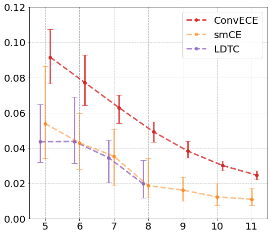
Figure 1: The $25\%$ quantile, median, and $75\%$ quantile (over $100$ runs) for ${\mathsf{smCE}}$, ${\underline{\mathsf{dCE}}}$ and ${\mathsf{cECE}}$ respectively. The $x$-axis is for dataset with size $2^{x}+1$.

Postprocessed neural networks.

In [GPSW17], which observed modern deep neural networks may be very miscalibrated, various strategies were proposed for postprocessing network predictions to calibrate them. We evaluate two of these strategies using our testing algorithms. We trained a DenseNet40 model [HLvdMW17] on the CIFAR-100 dataset [Kri09], producing a distribution $\mathcal{D}_{\textup{base}}$, where a draw $(v,y)\sim\mathcal{D}_{\textup{base}}$ selects a random example from the test dataset, sets $y$ to be its label, and $v$ to be the prediction of the neural network. We also learned calibrating postprocessing functions $f_{\textup{iso}}$ and $f_{\textup{temp}}$ from the training dataset, the former via isotonic regression and the latter via temperature scaling. These induce (ideally, calibrated) distributions $\mathcal{D}_{\textup{iso}}$, $\mathcal{D}_{\textup{temp}}$, where a draw from $\mathcal{D}_{\textup{iso}}$ samples $(v,y)\sim\mathcal{D}_{\textup{base}}$ and returns $(f_{\textup{iso}}(v),y)$, and $\mathcal{D}_{\textup{temp}}$ is defined analogously. The neural network and postprocessing functions were all trained by adapting code from [GPSW17].

We computed the median smooth calibration error of $20$ runs of the following experiment. In each run, for each $\mathcal{D}\in\{\mathcal{D}_{\textup{base}},\mathcal{D}_{\textup{iso}},\mathcal{D}_{\textup{temp}}\}$, we drew $4864$ random examples from $\mathcal{D}$, and computed the smooth calibration error ${\mathsf{smCE}}$ of the empirical dataset. We report our findings in Table 2.

$\mathcal{D}$	$\mathcal{D}_{\textup{base}}$	$\mathcal{D}_{\textup{iso}}$	$\mathcal{D}_{\textup{temp}}$
Empirical ${\mathsf{smCE}}$	$0.2269$	$0.2150$	$0.1542$

Table 2: Empirical ${\mathsf{smCE}}$ on postprocessed DenseNet40 predictions (median over $20$ runs)

Qualitatively, our results (based on ${\mathsf{smCE}}$) agree with findings in [GPSW17] (based on binned variants of $\mathsf{ECE}$), in that temperature scaling appears to be the most effective postprocessing technique.

${\mathsf{smCE}}$ tester.

Finally, we implemented our algorithm from Section 3, based on the minimax solver from [JT23]. We considered two types of augmented Lagrangian relaxations of the hard constraints, based on the sets of constraints $S_{\textup{base}}$ (defined in (20)) and $S_{0}$ (defined in (21)). In each case, we scaled up the Lagrangian penalty term by $\log_{2}(n-1)$. As described in Section 3.2, when using $S_{\textup{base}}$, this provably yields a soft-constrained empirical ${\mathsf{smCE}}$ objective which has the same value as the empirical ${\mathsf{smCE}}$ linear program. When using $S_{0}$, the objective guarantee is no longer provable, but we conduct this experiment because of the sufficiency of $S_{0}$ under hard constraints (see Lemma 7).

In Tables 3 and 4, we report the average suboptimality gap (across $5$ runs) using soft-penalized objectives based on $S_{0}$ and $S_{\textup{base}}$ respectively, varying the sample size and the number of iterations. The dataset is the same synthetic dataset based on Bernoulli samples as described earlier, with $\varepsilon^{\star}=0.1$. We scaled the number of iterations $T$ as multiples of $\sqrt{n}$, because this is the $\varepsilon^{-1}$ value suggested by our lower bound in Lemma 2. We find that both $S_{0}$ and $S_{\textup{base}}$ reliably converge to the empirical ${\mathsf{smCE}}$ computed by CVXPY, at the $\frac{1}{T}$ rate guaranteed by [JT23]. While $S_{\textup{base}}$ works better than $S_{0}$, there is not a large gap in their performance, suggesting it may be better to use $S_{0}$ in practice for efficiency. The constant $48$ was chosen based on parameters in [JT23]’s algorithm.

Finally, we note that a limitation of our work is that for these moderate values of $n$, our preliminary unoptimized code is slower than CVXPY’s custom linear program solver for ${\mathsf{smCE}}$. We find it encouraging that Tables 3, 4 demonstrate high levels of accuracy for small iteration counts $\approx 100$, and leave more efficient practical implementations as an important open direction.

$T$	$2^{5}+1$	$2^{6}+1$	$2^{7}+1$	$2^{8}+1$	$2^{9}+1$
$4.8\sqrt{n}$	$0.04789$	$0.03096$	$0.01829$	$0.01380$	$0.01006$
$24\sqrt{n}$	$0.01206$	$0.00719$	$0.00478$	$0.00314$	$0.00236$
$48\sqrt{n}$	$0.00657$	$0.00389$	$0.00267$	$0.00170$	$0.00139$

Table 3: Average suboptimality gap compared to CVXPY in $T$ iterations of [JT23] solver, using penalty based on $S_{0}$ constraints, across $5$ runs. Columns indicate sample size $n$.

$T$	$2^{5}+1$	$2^{6}+1$	$2^{7}+1$	$2^{8}+1$	$2^{9}+1$
$4.8\sqrt{n}$	$0.04203$	$0.02793$	$0.01797$	$0.01217$	$0.00959$
$24\sqrt{n}$	$0.00886$	$0.00583$	$0.00359$	$0.00192$	$0.00559$
$48\sqrt{n}$	$0.00443$	$0.00279$	$0.00180$	$0.00122$	$0.00096$

Table 4: Average suboptimality gap compared to CVXPY in $T$ iterations of [JT23] solver, using penalty based on $S_{\textup{base}}$ constraints, across $5$ runs. Columns indicate sample size $n$.

References

- [AAA+16] Dario Amodei, Sundaram Ananthanarayanan, Rishita Anubhai, Jingliang Bai, Eric Battenberg, Carl Case, Jared Casper, Bryan Catanzaro, Jingdong Chen, Mike Chrzanowski, Adam Coates, Greg Diamos, Erich Elsen, Jesse H. Engel, Linxi Fan, Christopher Fougner, Awni Y. Hannun, Billy Jun, Tony Han, Patrick LeGresley, Xiangang Li, Libby Lin, Sharan Narang, Andrew Y. Ng, Sherjil Ozair, Ryan Prenger, Sheng Qian, Jonathan Raiman, Sanjeev Satheesh, David Seetapun, Shubho Sengupta, Chong Wang, Yi Wang, Zhiqian Wang, Bo Xiao, Yan Xie, Dani Yogatama, Jun Zhan, and Zhenyao Zhu. Deep speech 2 : End-to-end speech recognition in english and mandarin. In Proceedings of the 33nd International Conference on Machine Learning, ICML 2016, volume 48 of JMLR Workshop and Conference Proceedings, pages 173–182. JMLR.org, 2016.
- [AVDB18] Akshay Agrawal, Robin Verschueren, Steven Diamond, and Stephen Boyd. A rewriting system for convex optimization problems. Journal of Control and Decision, 5(1):42–60, 2018.
- [BGHN23a] Jarosław Błasiok, Parikshit Gopalan, Lunjia Hu, and Preetum Nakkiran. A unifying theory of distance from calibration. In Proceedings of the 55th Annual ACM Symposium on Theory of Computing, pages 1727–1740, 2023.
- [BGHN23b] Jarosław Błasiok, Parikshit Gopalan, Lunjia Hu, and Preetum Nakkiran. When does optimizing a proper loss yield calibration? arXiv preprint arXiv:2305.18764, 2023.
- [BN23] Jarosław Błasiok and Preetum Nakkiran. Smooth ECE: Principled reliability diagrams via kernel smoothing. arXiv preprint arXiv:2309.12236, 2023.
- [Can22] Clément L. Canonne. Topics and techniques in distribution testing: A biased but representative sample. Foundations and Trends® in Communications and Information Theory, 19(6):1032–1198, 2022.
- [CLS21] Michael B. Cohen, Yin Tat Lee, and Zhao Song. Solving linear programs in the current matrix multiplication time. J. ACM, 68(1):3:1–3:39, 2021.
- [CST21] Michael B. Cohen, Aaron Sidford, and Kevin Tian. Relative lipschitzness in extragradient methods and a direct recipe for acceleration. In 12th Innovations in Theoretical Computer Science Conference, ITCS 2021, volume 185 of LIPIcs, pages 62:1–62:18. Schloss Dagstuhl - Leibniz-Zentrum für Informatik, 2021.
- [DB16] Steven Diamond and Stephen Boyd. CVXPY: A Python-embedded modeling language for convex optimization. Journal of Machine Learning Research, 17(83):1–5, 2016.
- [DKR+21] Cynthia Dwork, Michael P. Kim, Omer Reingold, Guy N. Rothblum, and Gal Yona. Outcome indistinguishability. In STOC ’21: 53rd Annual ACM SIGACT Symposium on Theory of Computing, 2021, pages 1095–1108. ACM, 2021.
- [Doi07] Kunio Doi. Computer-aided diagnosis in medical imaging: historical review, current status and future potential. Computerized medical imaging and graphics, 31(4–5):198–211, 2007.
- [GKR+22] Parikshit Gopalan, Adam Tauman Kalai, Omer Reingold, Vatsal Sharan, and Udi Wieder. Omnipredictors. In 13th Innovations in Theoretical Computer Science Conference, ITCS 2022, volume 215 of LIPIcs, pages 79:1–79:21. Schloss Dagstuhl - Leibniz-Zentrum für Informatik, 2022.
- [Gol17] Oded Goldreich. Introduction to Property Testing. Cambridge University Press, 2017.
- [GPSW17] Chuan Guo, Geoff Pleiss, Yu Sun, and Kilian Q Weinberger. On calibration of modern neural networks. In International conference on machine learning, pages 1321–1330. PMLR, 2017.
- [HKRR18] Úrsula Hébert-Johnson, Michael P. Kim, Omer Reingold, and Guy N. Rothblum. Multicalibration: Calibration for the (computationally-identifiable) masses. In Proceedings of the 35th International Conference on Machine Learning, ICML 2018, volume 80 of Proceedings of Machine Learning Research, pages 1944–1953. PMLR, 2018.
- [HLvdMW17] Gao Huang, Zhuang Liu, Laurens van der Maaten, and Kilian Q. Weinberger. Densely connected convolutional networks. In 2017 IEEE Conference on Computer Vision and Pattern Recognition, CVPR 2017, pages 2261–2269. IEEE Computer Society, 2017.
- [IS03] Y. I. Ingster and I. A. Suslina. Nonparametric Goodness-of-Fit Testing under Gaussian Models, volume 169 of Lecture Notes in Statistics. Springer-Verlag, New York, 2003.
- [JST19] Arun Jambulapati, Aaron Sidford, and Kevin Tian. A direct iteration parallel algorithm for optimal transport. Advances in Neural Information Processing Systems, 32, 2019.
- [JT23] Arun Jambulapati and Kevin Tian. Revisiting area convexity: Faster box-simplex games and spectrahedral generalizations. arXiv preprint arXiv:2303.15627, 2023.
- [KF04] Sham M. Kakade and Dean P. Foster. Deterministic calibration and nash equilibrium. In John Shawe-Taylor and Yoram Singer, editors, Learning Theory, pages 33–48, Berlin, Heidelberg, 2004. Springer Berlin Heidelberg.
- [KF08] Sham M. Kakade and Dean P. Foster. Deterministic calibration and nash equilibrium. J. Comput. Syst. Sci., 74(1):115–130, 2008.
- [KLM19] Ananya Kumar, Percy Liang, and Tengyu Ma. Verified uncertainty calibration. In Advances in Neural Information Processing Systems 32: Annual Conference on Neural Information Processing Systems 2019, NeurIPS 2019, pages 3787–3798, 2019.
- [Kri09] Alex Krizhevsky. Learning multiple layers of features from tiny images. https://www.cs.toronto.edu/ kriz/learning-features-2009-TR.pdf, 2009. Accessed: 2024-01-31.
- [KSJ18] Aviral Kumar, Sunita Sarawagi, and Ujjwal Jain. Trainable calibration measures for neural networks from kernel mean embeddings. In Jennifer Dy and Andreas Krause, editors, Proceedings of the 35th International Conference on Machine Learning, volume 80 of Proceedings of Machine Learning Research, pages 2805–2814. PMLR, 10–15 Jul 2018.
- [LeC73] L. LeCam. Convergence of Estimates Under Dimensionality Restrictions. The Annals of Statistics, 1(1):38 – 53, 1973.
- [LS14] Yin Tat Lee and Aaron Sidford. Path finding methods for linear programming: Solving linear programs in õ(vrank) iterations and faster algorithms for maximum flow. In 55th IEEE Annual Symposium on Foundations of Computer Science, FOCS 2014, pages 424–433. IEEE Computer Society, 2014.
- [MDR+21a] Matthias Minderer, Josip Djolonga, Rob Romijnders, Frances Hubis, Xiaohua Zhai, Neil Houlsby, Dustin Tran, and Mario Lucic. Revisiting the calibration of modern neural networks. In Advances in Neural Information Processing Systems 34: Annual Conference on Neural Information Processing Systems 2021, pages 15682–15694, 2021.
- [MDR+21b] Matthias Minderer, Josip Djolonga, Rob Romijnders, Frances Hubis, Xiaohua Zhai, Neil Houlsby, Dustin Tran, and Mario Lucic. Revisiting the calibration of modern neural networks. In M. Ranzato, A. Beygelzimer, Y. Dauphin, P.S. Liang, and J. Wortman Vaughan, editors, Advances in Neural Information Processing Systems, volume 34, pages 15682–15694. Curran Associates, Inc., 2021.
- [Mur98] Allan H. Murphy. The early history of probability forecasts: Some extensions and clarifications. Weather and forecasting, 13(1):5–15, 1998.
- [MW84] Allan H. Murphy and Robert L. Winkler. Probability forecasting in meteorology. Journal of the American Statistical Association, 79(387):489–500, 1984.
- [NCH15] Mahdi Pakdaman Naeini, Gregory F. Cooper, and Milos Hauskrecht. Obtaining well calibrated probabilities using bayesian binning. In Proceedings of the Twenty-Ninth AAAI Conference on Artificial Intelligence, January 25-30, 2015, pages 2901–2907. AAAI Press, 2015.
- [NDZ+19] Jeremy Nixon, Michael W. Dusenberry, Linchuan Zhang, Ghassen Jerfel, and Dustin Tran. Measuring calibration in deep learning. In IEEE Conference on Computer Vision and Pattern Recognition Workshops, CVPR Workshops 2019, pages 38–41. Computer Vision Foundation / IEEE, 2019.
- [Nie22] Zipei Nie. Matrix anti-concentration inequalities with applications. In STOC ’22: 54th Annual ACM SIGACT Symposium on Theory of Computing, pages 568–581. ACM, 2022.
- [PV21] Richard Peng and Santosh S. Vempala. Solving sparse linear systems faster than matrix multiplication. In Proceedings of the 2021 ACM-SIAM Symposium on Discrete Algorithms, SODA 2021, pages 504–521. SIAM, 2021.
- [Ron08] Dana Ron. Property testing: A learning theory perspective. Found. Trends Mach. Learn., 1(3):307–402, 2008.
- [Ron09] Dana Ron. Algorithmic and analysis techniques in property testing. Found. Trends Theor. Comput. Sci., 5(2):73–205, 2009.
- [RRSK11] Francesco Ricci, Lior Rokach, Bracha Shapira, and Paul B. Kantor. Recommender Systems Handbook. Springer New York, 2011.
- [Rt21a] Rahul Rahaman and alexandre thiery. Uncertainty quantification and deep ensembles. In M. Ranzato, A. Beygelzimer, Y. Dauphin, P.S. Liang, and J. Wortman Vaughan, editors, Advances in Neural Information Processing Systems, volume 34, pages 20063–20075. Curran Associates, Inc., 2021.
- [RT21b] Rahul Rahaman and Alexandre H. Thiéry. Uncertainty quantification and deep ensembles. In Advances in Neural Information Processing Systems 34: Annual Conference on Neural Information Processing Systems 2021, pages 20063–20075, 2021.
- [She13] Jonah Sherman. Nearly maximum flows in nearly linear time. In 54th Annual IEEE Symposium on Foundations of Computer Science, FOCS 2013, pages 263–269. IEEE Computer Society, 2013.
- [She17] Jonah Sherman. Area-convexity, l regularization, and undirected multicommodity flow. In Hamed Hatami, Pierre McKenzie, and Valerie King, editors, Proceedings of the 49th Annual ACM SIGACT Symposium on Theory of Computing, STOC 2017, pages 452–460. ACM, 2017.
- [vdBLL+21] Jan van den Brand, Yin Tat Lee, Yang P. Liu, Thatchaphol Saranurak, Aaron Sidford, Zhao Song, and Di Wang. Minimum cost flows, mdps, and -regression in nearly linear time for dense instances. In STOC ’21: 53rd Annual ACM SIGACT Symposium on Theory of Computing, 2021, pages 859–869. ACM, 2021.
- [vdBLSS20] Jan van den Brand, Yin Tat Lee, Aaron Sidford, and Zhao Song. Solving tall dense linear programs in nearly linear time. In Proceedings of the 52nd Annual ACM SIGACT Symposium on Theory of Computing, STOC 2020, pages 775–788. ACM, 2020.
- [VDDP17] Athanasios Voulodimos, Nikolaos Doulamis, Anastasios Doulamis, and Eftychios Protopapadakis. Deep learning for computer vision: A brief review. Computational Intelligence and Neuroscience, 2018, 2017.
- [WXXZ23] Virginia Vassilevska Williams, Yinzhan Xu, Zixuan Xu, and Renfei Zhou. New bounds for matrix multiplication: from alpha to omega. CoRR, abs/2307.07970, 2023.